Evaluation of the Performance and the Predictive Capacity of Build-Up and Wash-Off Models on Different Temporal Scales

Abstract

Stormwater quality modeling has arisen as a promising tool to develop mitigation strategies. The aim of this paper is to assess the build-up and wash-off processes and investigate the capacity of several water quality models to accurately simulate and predict the temporal variability of suspended solids concentrations in runoff, based on a long-term data set. A Markov Chain Monte-Carlo (MCMC) technique is applied to calibrate the models and analyze the parameter’s uncertainty. The short-term predictive capacity of the models is assessed based on inter- and intra-event approaches. Results suggest that the performance of the wash-off model is related to the dynamic of pollutant transport where the best fit is recorded for first flush events. Assessment of SWMM (Storm Water Management Model) exponential build-up model reveals that better performance is obtained on short periods and that build-up models relying only on the antecedent dry weather period as an explanatory variable, cannot predict satisfactorily the accumulated mass on the surface. The predictive inter-event capacity of SWMM exponential model proves its inability to predict the pollutograph while the intra-event approach based on data assimilation proves its efficiency for first flush events only. This method is very interesting for management practices because of its simplicity and easy implementation.

1. Introduction

Growing urbanization increases stormwater runoff on impervious surfaces and pollutant loads leading to a tremendous ecological footprint [1]. Nonpoint source pollution discharged during rainfall events into receiving water bodies carries a high load of contaminants, including microorganisms, PAHs (Polycyclic aromatic hydrocarbon), metals and other anthropogenic contaminants, mainly adsorbed onto suspended solids in runoff [2,3,4]. Pollutants accumulate on urban catchments during dry weather periods and are mostly generated by anthropogenic activities but also by atmospheric deposition and re-suspension of the surrounding soil [5,6,7,8]. These pollutants are washed off by storm events where the particles are eroded and detached by rainfall drops and transported by runoff into the drainage network [9,10]. Several dynamics of pollutant transport exist and attempt to explain the variations in pollutant concentrations through the stages of runoff [11]. The fluctuations of the pressure exerted thus on ecosystems must be quantified including the accurate knowledge of the underlying processes of generation and transport of pollutants, in order to preserve the receiving environments from deterioration as well as meeting the legislative requirements imposed by the European Water Framework Directive [12]. Mitigation strategies include continuous monitoring of experimental sites. However, the high expenses involved in this approach bring to light the necessity to find a more appropriate alternative that can be transposed on unmonitored catchments. Hence, mathematical models have arisen as a promising tool to predict and simulate runoff quantity and quality since the 1970s [13,14].

Water quality models simulate pollutant loads based either on statistical regression equations or on conceptual and physical ones, replicating the processes of build-up and wash-off. Regression models rely on simple statistical methods that relate pollutant concentrations and loads to explanatory variables such as rainfall, runoff and catchment characteristics [15,16]. Even though regression equations are of interest for estimating total pollutant loads on the event and annual scale, they are not very reliable when they are applied at a small time step [16] and can hardly be transferred from a catchment to another since they are calibrated using a data set specific to one particular catchment. Process based models consist mainly of replicating the deposition of pollutants on surfaces between two storm events and their removal and transport by the rain [10,14,17]. Both conceptual and physical approaches have been developed and tested in order to achieve the best simulation of the pollutograph at the outlet of catchments.

Physical approaches developed for modeling the wash-off process usually consider the replication of the erosion of accumulated sediments on the surface, driven by the rainfall impact and the overland flow, as well as their deposition [18]. Shaw et al. [9] proposed in their study a saltation mechanistic wash-off model that describes the detachment of pollutant loads by raindrop while Massoudieh et al. [19] simulated pollutant concentrations using a wash-off model that includes the detachment and reattachment processes. In a recent study, Hong et al. [20] developed a physical model that considers both rainfall impact and overland flow as the driving mechanism of sediment erosion and suggested that raindrop is the major actor in detaching sediments of the urban surface. Physical approaches are very useful to have an in depth insight into the corresponding process, however, the implementation of physically based models is not always possible especially if they are destined for operational use because they require the availability of large data sets that answer to the detailed description of the system. The large number of parameters also implicated in the model structure require an extensive calibration, thus it is time consuming. These reasons among others orient more toward the application of conceptual approaches. Conceptual build-up models are usually formulated as a function of antecedent dry weather period and are represented either by linear, power, exponential or the Michaelis–Menton equations [17,21,22,23]. As for wash-off, it is mathematically modeled as an exponential decrease of initial available pollutant mass on the surface, function of rainfall intensity, runoff volume or runoff rate [22]. Recent studies shows that these models can successfully replicate pollutant loads [24,25,26] but not the temporal variability of pollutant concentrations [13,19,27]. An in depth investigation based on a reliable and significant data set might be the answer to better understand the issue of accurate concentration estimates: the still unconquered holy grail of this field.

Therefore, the main purpose of this research is to evaluate the build-up and wash-off processes and investigate the capacity of commonly used water quality models to accurately simulate total suspended solids concentrations (TSS) and reproduce their temporal variability in runoff, based on a long-term, continuous data set. First, a wash-off model is evaluated and its performance is discussed with respect to different dynamics of pollutant transport to identify whether its applicability is specific to a certain type of events. Then two build-up models are evaluated in order to test their ability of replicating the accumulation of pollutants on urban surfaces in realistic conditions. Model calibration is performed based on the “Markov Chain Monte Carlo” technique, which enables the assessment of uncertainty associated with the model parameters. Finally, the short term predictive capacity of the models is investigated first at the inter-event scale, to test the period length during which the characteristics of a calibrated model remain valid, then at the intra-event scale where a new methodology is developed based on data assimilation, where the observations of the ongoing event are used for calibrating the available pollutant mass for erosion.

2. Materials and Methods

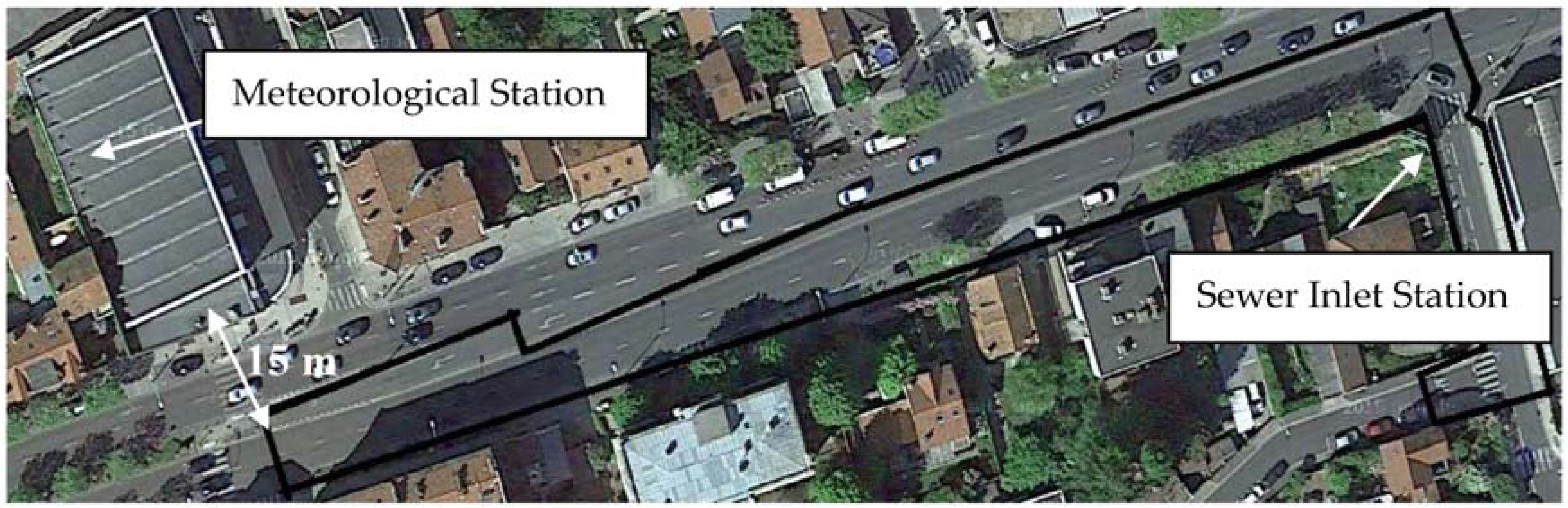
2.1. Experimental Site and Monitoring Equipment

The studied catchment is a 2661 m² road surface with its adjacent sidewalks, pavements and parking zones located in the residential French district “Le Perreux sur Marne”. The area carries high traffic loads (~30,000 vehicles per day) and is drained by a separate stormwater system. The catchment is characterized by an imperviousness equal to 70%, a runoff length of 167 m and an average slope of 2.6% (Figure 1).

From April 2014 to September 2015, monitoring systems were installed in the studied experimental site to monitor and sample rainfall and road runoff. In this research, data collected from June 2014 to April 2015 are exploited.

Precipitation data are collected from a meteorological station installed at 180 m from the road sewer inlet and at 15 m from the catchment’s extremity; 10 mL tipping bucket rain gauge is used for rainfall measurements, which corresponds to a resolution of 0.1 mm of precipitation height. The station was not installed directly on the road catchment to avoid its deterioration by the pedestrians and the surrounding activities and also to reduce the risk of technical problems that will induce significant errors in the measurements.

The monitoring devices of flow and water quality parameters for road runoff are located in the sewer inlet into the drainage system and recorded measurements at 1 min time step. For flow measurement, a Nivus flow meter, based on cross correlation method and providing high accurate ultrasonic flow measurements is used. As for quality aspects, turbidity (NTU), conductivity, pH and temperature are monitored with a DS5 OTT multi-parameter probe. For reasons of power and storage savings, the setting off probe was triggered by the flow meter. Once the flow is higher than 0.15 L/s (which is considered as the limit of measurement of the flow meter) the quality measurements are launched until the flow becomes lower than 0.13 L/s for more than 15 min. Systematic volume of 500 mL are also collected for further laboratory analysis of metals, PAHs, DOC (Dissolved organic carbon), POC (Particulate organic carbon) and TSS for some rainfall events. For each event, the volume is pumped into two bottles (one made of glass and one made of plastic) of 20 L capacity; 250 mL are pumped into each one placed in a closed box on the sidewalk by a peristaltic pump (Watson-Marlow, Falmouth, Cornwall, UK), for each 300 L passing through the system. This volume was determined for covering 100% of most rainfall events, being thus representative of the total load during the rainfall event.

Linear relationship between turbidity and Total Suspended Solids is established in order to convert turbidity measurements into TSS concentrations. The TSS–turbidity relationship is calculated using measurements of turbidity obtained from nine samples. TSS concentrations are quantified by filtration, using 0.45 µm filters composed of glass fibers. Distinction between the metallic and the organic content of sediments is not considered. Thus the linear regression function adjusted over nine storm events, with a correlation factor R² = 0.98, is given by:

TSS = 0.9006 × T

(1)

where TSS is the concentration of Total Suspended Solids in mg/L; and T is Turbidity in NTU.

2.2. Data Set

Overall, 246 rainfall events are recorded for the period between June 2014 and April 2015. Rainfall events are defined as uninterrupted measurement periods, during which the maximum time between bucket tips is 30 min. The precision of the rain gauge is 0.1 mm. The review of the collected meteorological data indicates extensive variability of rainfall characteristics (

Table 1. Statistics of the 286 recorded storm events.

Rainfall Characteristic	Rainfall Depth (mm)	Duration (min)	ADWP (DD HH:MM:SS)	Maximum 1 min Intensity (mm/h)	Maximum 5 min Intensity (mm/h)	Maximum Intensity (mm/h)	Average Intensity (mm/h)
Max	21.3	641.1	21 05:28:19	131	100.2	360	53.9
Min	0.2	0.8	00 00:30:14	0.2	0.2	0.2	0.4
Median	0.7	34.78	00 06:47:05	3.03	2.31	2.94	1.36
Mean	2.128	75.2	01 06:14:24	9.19	6.61	14.09	3.25

).

Most storm events are short, as 50% of the events did not last for more than 35 min. The total rainfall depth varies from 0.2 to 21.3 mm, while maximum rainfall intensities varies between 0.2 mm/h and 360 mm/h. It is noteworthy that the median value of the antecedent dry weather period is 6 h indicating short time interval separating rainfall events; hence, the occurrence of successive storms. Fifty-four storms did not generate runoff, and precipitations in this case fulfilled initial losses.

Runoff data on the corresponding period are recorded for 187 events and were missing for five events due to technical problems, while turbidity measurements are recorded for 106 events on which water quality characteristics (event mean concentrations and loads) are assessed.

2.3. Data Validation

2.3.1. Turbidity

A crucial point in urban stormwater modeling is the quality of the data set used, since it is reflected in the quality of the results. Raw measurements obtained directly from site monitoring cannot be used before undergoing a validation procedure in order to eliminate non reliable measurements and interpolating when possible missing data points [28,29]. Automatic pre-validation is first developed to highlight wrong and doubtful data by associating a mark that reflects the validity of each measurement of turbidity, followed by a final manual validation. The technique is inspired by the work of Mourad and Bertrand-Krajewski [29] and the software EVOHE [30] but modified to fit this study case since turbidity measurements are obtained using one turbidimeter at the inlet of the drainage network.

The automatic pre-validation consists of several steps. First, initial marks are given to all turbidity measurements based on the sensor measurement range as follows:

• if the measurement is between the minimum and the maximum values given by the turbidity sensors, which are 0 and 3000, respectively;
• if the measurement is equal to the saturated value 3000;
• if the measurement is negative or equal to zero or recorded during intervention on site for maintenance operations.

Negative and zero values of turbidity are then interpolated and re-flagged 1 if they are recorded intra-event for three consecutive minutes or less. Finally, the values that exceeded the 99.5th percentile of global signal’s gradient are considered as abnormal and marked 4. These measurements indicate sudden and irregular change in the signal that cannot be related to any physical process. All data that have a valid flag (i.e., equal to 1) at the end of the process are kept for the analysis. Others are checked for final validation manually by comparing rainfall, flow and turbidity graphs. If the saturated values or the values due to a high gradient, marked initially as 2 and 4, are coincident with a high rainfall intensity and high flow they are finally re-marked as 1 and taken as valid measurements. All data whose flag are different than 1 at the end of the manual validation were reflagged 2.

The above procedure generates a validated data set and is efficient in detecting the wrong and doubtful data that may induce errors in modeling results. In fact, these errors are noticed when comparing the Nash–Sutcliffe coefficients when calibrating on several events before and after the manual validation. False turbidity peaks that were kept after the automatic validation for the events of 14 and 15 November 2014, for example, clearly affected the calibration of the model. The Nash–Sutcliffe efficiencies obtained then were 0.03 and 0.55 respectively and they were highly improved after the removal of the mistaken turbidity values, Nash–Sutcliffe coefficients increased to 0.47 and 0.87, proving the sensibility of the model toward false measurements.

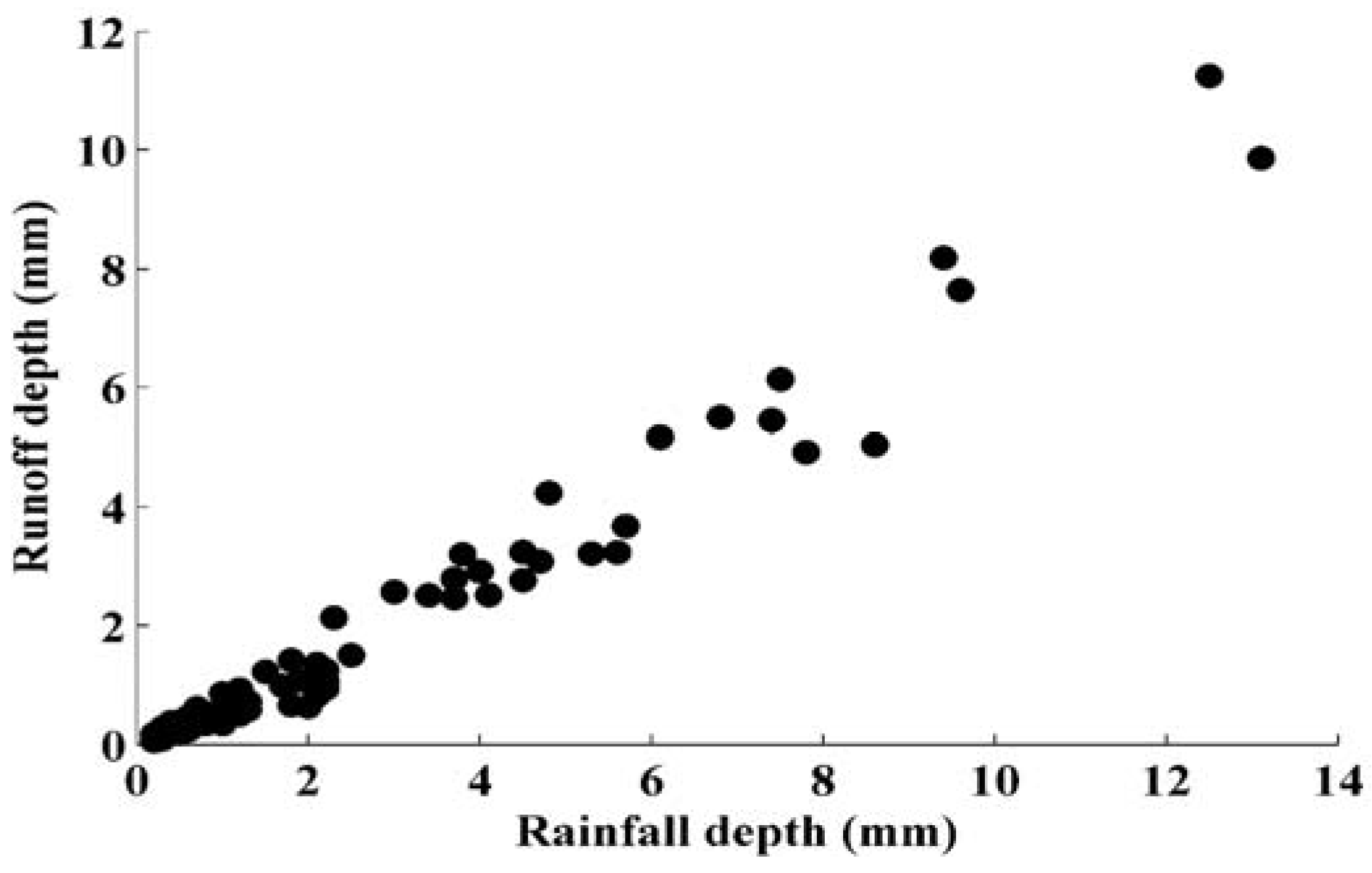
2.3.2. Hydrological Modeling

Flow measurements are validated by calculating the global runoff coefficient as well as the runoff coefficients for each event. Global runoff coefficient is equal to 0.73, calculated by taking into account the initial losses that correspond to 0.5 mm. The initial losses are defined as mean rainfall depths that never generated any runoff. Runoff coefficients for each event are variable and the initial loss is calculated for each event apart. This variability is noticed when plotting the runoff depth function of rainfall depth (Appendix A, Figure A1). Precipitations with the same rainfall depth will result in different runoff depth, due to several factors including dry weather period, evaporation and depression storage. The events resulting in runoff coefficients greater than one are modeled in addition to the missing runoff data due to technical problems. A hydrological model consisting of a non-linear reservoir is calibrated and validated over 102 events using rainfall data of the rain gauge on site to substitute the lost records. The model replicates accurately the flow measurements with a Nash–Sutcliffe efficiency of 0.85.

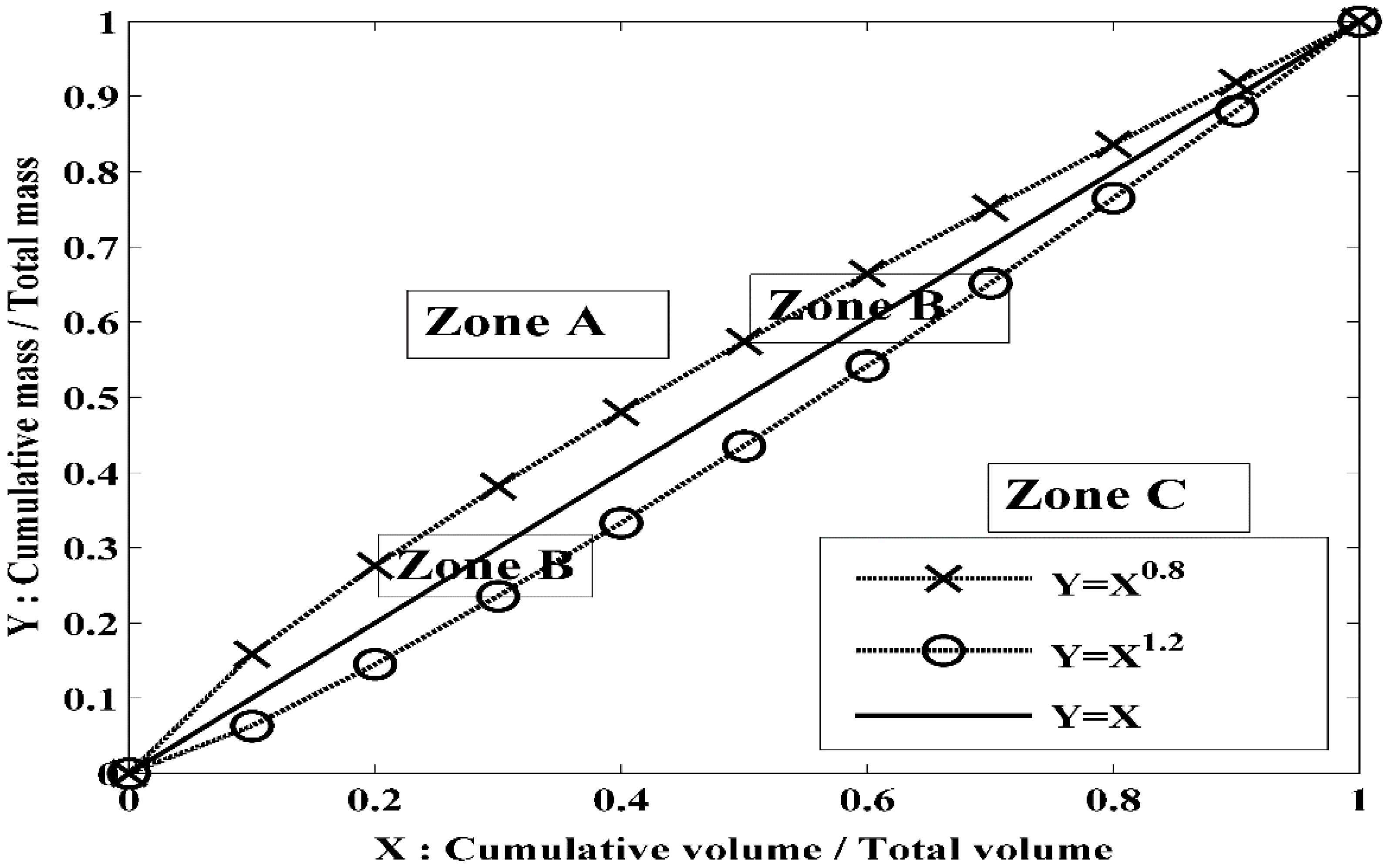
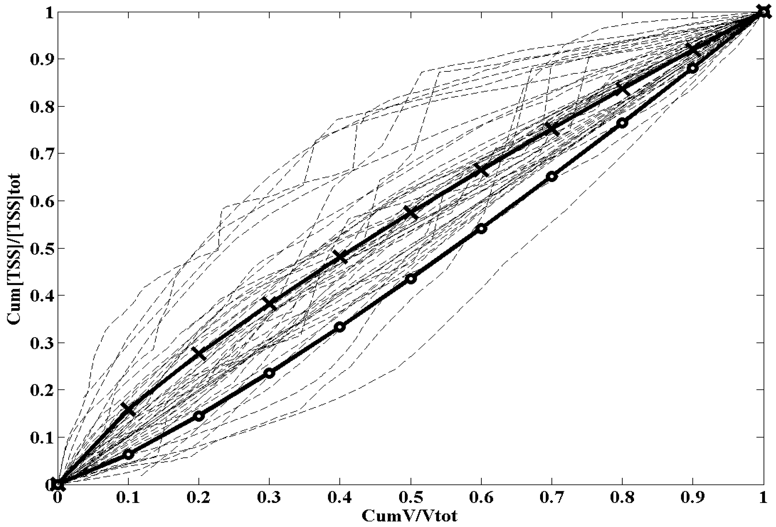
2.4. Intra-Event Dynamic of TSS Transport

In order to distinguish the different dynamics of TSS transport during a rainfall event, dimensionless M (V) curves are plotted. Three typology of events (first flush, last flush and uniformly distributed) delimited by three zones A, B and C (Figure 2) are defined based on a simplified classification of the M (V) curves inspired by the method proposed earlier by Bertrand-Krajewski et al. [11]. Simplifications are made since the definition of first flush given by these authors is very restrictive and given in the perspective of designing treatment facilities, while in our case a less restrictive definition is needed.

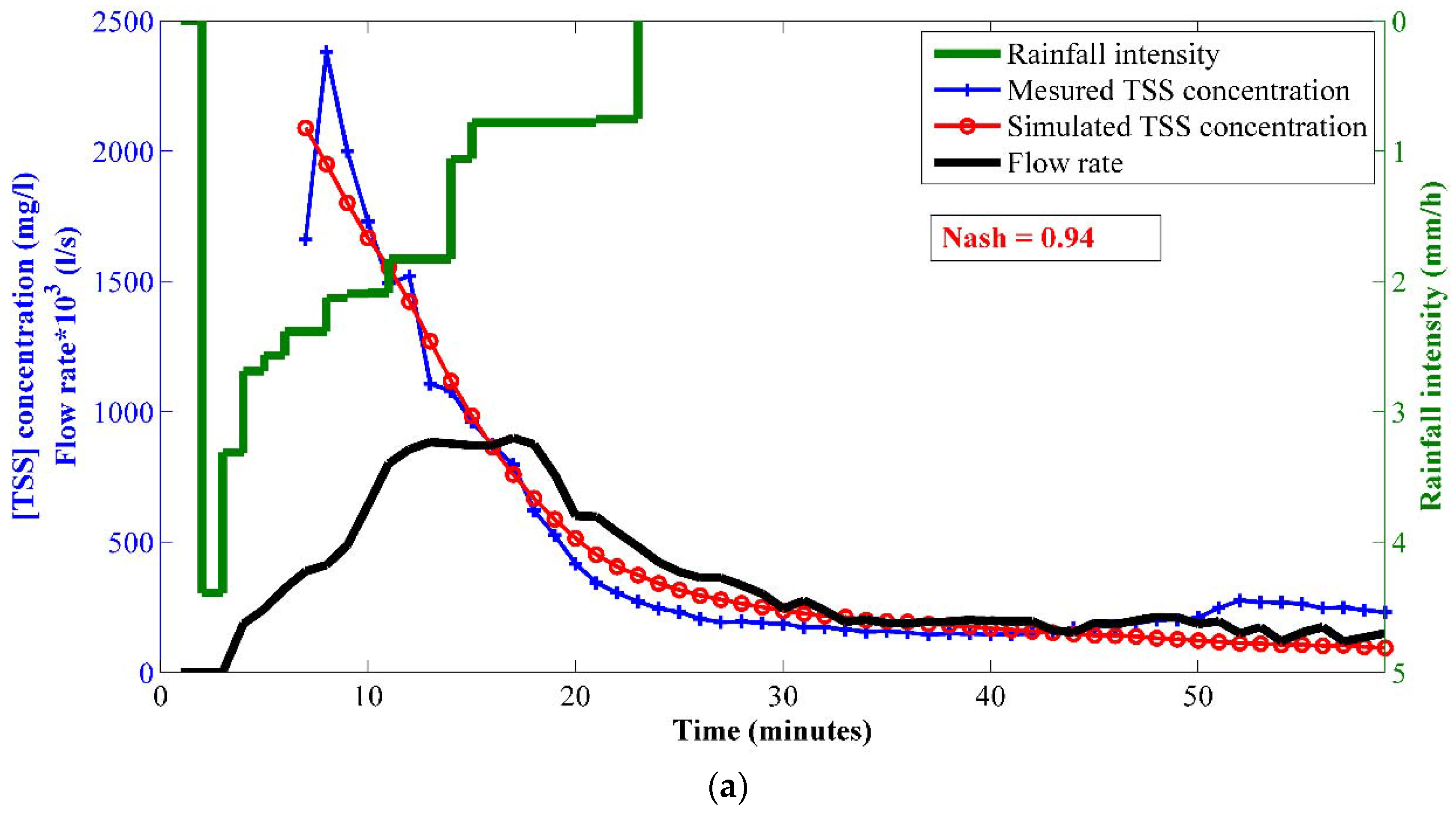
2.5. Water Quality Modeling

2.5.1. The Models

Numerous modeling approaches for pollutant generation and transport exist and are detailed and compared in several reviews [1,31,32]. These reviews classify stormwater quality models based on modeling approaches, process description, and spatial and temporal scales (

Table 2. General classification of stormwater quality models based on different criteria.

Criteria of Classification	Model Type	Description
Variable description	Deterministic	Variables properties are well known and do not include any randomness. The same input will yield the same output.
	Stochastic	Variables have a probability distribution and its uncertainty is built into the model. The same input will yield different possible outputs.
Process description	Empirical	Relations between inputs and outputs are established from observations only without any intervention of physical laws
	Conceptual	Physical laws are applied in simple and simplified form
	Physically based	Logical structure based on physical laws governing the process
Spatial scale	Global (lumped)	Catchment is described as a whole entity
	Semi distributed	Catchment is divided into sub catchment
	Distributed	Catchment is divided into elementary unit using a grid
Temporal scale	Event	Individual events are simulated
	Continuous	Long period of time are simulated

). In this study, we chose conceptual models to replicate the build-up and wash-off processes since they are easily implemented and simply applicable thus more attractive for practical applications. In addition, the diversity of the performance of these models emerging from past researches supports the need for further investigation of these formulations. Thus, we benefit from the extensive data set available on this site to test different models and contribute in the comprehension of build-up and wash-off processes.

We investigated two pollutant build-up models: the exponential build-up model of SWMM (Storm Water Management Model) and a power function. The exponential build-up model describes an exponential growth of the build-up curve until it reaches asymptotically the upper limit, which corresponds to the maximum pollutant load that can be accumulated on the surface. This limit is reached at the equilibrium state between deposition and removal of pollutant particle [17]. The remaining pollutant load from the previous rainfall event is also taken into account. The amount of build-up at the beginning of the rainfall event M_B (g/m²) is thus computed using the first order exponential equation:

M_B(i) = D_ACCU/D_ERO × [1 − e^{(−DERO × ADWP (i))}] + M_RES. e^{(−DERO × ADWP(i))}

(2)

where M_RES is the remaining pollutant load mass from the previous rainfall event (g/m²); ADWP_(i) is the antecedent dry weather period preceding the event i (day); D_ACCU is the pollutant accumulation rate (g/m²/day); and D_ERO is the pollutant erosion rate (/day).

The other model used to describe the accumulation process is based on the power function [21]. The pollutant load M_B (g/m²) present on the surface prior to a storm event is computed as follows:

M_B = a.ADWP^b_(i)

(3)

where a and b are build-up coefficients

This model assumes that the build-up process starts from zero and that the previous storm event erodes off all the pollutant present on the surface. Even though recent studies showed that a rainfall event washes away only a fraction of the pollutants available [10,33], this model gave the best results in replicating pollutant loads collected from experimental data [21,34].

Pollutant wash-off is simulated using the modified exponential model of SWMM [22], which considers the non-linear relation between the wash-off load and the runoff rate. This relation is taken into account by introducing the wash-off exponent C2, which was initially set to be equal to one in the original SWMM version suggesting a linear dependency of the washed off fraction on the runoff rate. The eroded pollutant mass at time t during a storm event is calculated thus with the following equation:

M_ERO (t) = M_B(t).C1.q(t)^C2.dt

(4)

M_B(t + dt) = M_B(t) − M_ERO (t)

(5)

where M_ERO(t) is the eroded pollutant mass at t during the time step dt (g/m²); M_B(t) is the available pollutant mass for erosion at time t (g/m²); q(t) is the runoff rate (mm/h); dt is the time step; C1 is the wash-off coefficient; and C2 is the wash-off exponent.

2.5.2. Calibration

Application of water quality models requires estimation of build-up and wash-off parameters, as these models have very low performance if not calibrated [35].

The exponential build-up model integrates three parameters D_ACCU, D_ERO and the initial pollutant load present on the surface M_{RES (t=0)}, whereas the power model integrates two parameters which are the build-up coefficients a and b. The exponential wash-off model requires the adjustment of two parameters C1 and C2. These parameters are adjusted using an automatic calibration technique based on the Bayesian approach. This approach allows the assessment of parameters uncertainty by estimating their posterior probability distribution P(θ/Y_obs) given by Bayes’ theorem and expressed as follow:

P(θ/Y_obs) α L(θ/Y_obs). P(θ)

(6)

where θ is a model parameter; Y_obs is the time series of observations; P(θ) is the prior probability distribution of the parameters; and L(θ/Y_obs) is the likelihood function that describes the statistical characteristics of residuals between the observations and the model outputs.

The posterior probability is calculated based on the Metropolis-Hastings algorithm [36] of the Monte Carlo Markov Chain sampling technique.

The assumptions made in this study for the implementation of the Bayesian approach in the calibrations of build-up and wash-off models are the same as those made in the previous work of Kanso et al. [27].

At the end of calibration process we obtain not only the set of parameters for which we have the maximum likelihood, and that corresponds to the optimal set of parameters, but also the posterior probability distribution of the parameters that provides information on the uncertainty associated to these parameters and the likelihood probability vs. the parameters that allows the computation of model sensibility toward the parameters and the assessment of the uniqueness of the given optimum parameter set. The model performance is also assessed using the Nash–Sutcliffe coefficient [37].

Calibration is performed considering the period starting from November 2014 to April 2015. First, it is performed on single event scale to evaluate the wash-off process. The available mass at the beginning of the rainfall event in this case is considered as a parameter and is calibrated along with the wash-off coefficient and exponent. Overall, 42 events are included and the results are analyzed distinguishing the three typology of events in order to investigate if the performance of the wash-off model is related to the dynamic of pollutant transport by runoff. Then calibration is performed on continuous periods consisting of three, six and nine successive events in order to evaluate the build-up process and check to which extent the build-up model can accurately predict the available mass between consecutive events. A total of 114 rainfall events are included. The configurations evaluated, couple the modified exponential SWMM build-up model, then the power build-up function with the SWMM wash-off model. A summary of the calibration procedure is presented in

Table 3. Calibration methodology of wash-off and build-up models.

Calibration	Wash-Off Assessment	Build-Up Assessment
Number of events	42	16 periods of 3 successive events each
		8 periods of 6 successive events each
		4 periods of 9 successive events each
Model	MERO (t) = MB(t).C1.q(t)C2.dt	MB (i) = DACCU/DERO × [1 − e(−DERO × ADWP (i))] + MRES. e(−DERO × ADWP(i))
		MB (i) = a.ADWPb(i)

.

2.5.3. Prediction on Short Term

The prediction capacity of the models on short term is also investigated to determine whether they can provide accurate predictions of the TSS concentrations over short periods of times. For that matter two approaches are investigated: inter-event and intra-event.

In the inter-event approach, 114 events are divided into periods of four events each; calibration is performed on the first two events and the models are validated on the third, and then on the third and fourth events simultaneously.

In the intra-event approach, observations are used along with the median value of wash-off parameters calibrated on first flush events to determine the available pollutant mass at the beginning of the storm. Then this mass is eroded by the storm and the Nash–Sutcliffe coefficient between the measured and the simulated TSS concentrations is calculated. The observations are included into the numerical model by a simple data assimilation technique. The number of points taken into account to calculate the available mass increase starting from two points up to considering the whole set of measurements. This allows identifying if the model can predict the total storm variation only if the first part of a storm is monitored. This method is applied on 38 events and a summary of the prediction methodology is presented in the table below (

Table 4. Prediction approaches: inter and intra event.

Prediction Approaches		Inter-Event Approach	Intra-Event Approach
Number of events		11 periods of 4 events each	38
Model	Build-up	MB (i) = DACCU/DERO × [1 − e(−DERO × ADWP (i))] + MRES. e(−DERO × ADWP(i))	-
		MB (i) = a.ADWPb(i)
	Wash-off	MERO (t) = MB(t).C1.q(t)C2.dt
Methodology		Calibration on the first two events of the period Validation on the third event of the corresponding period Validation on the third and the fourth events of the corresponding period	Calculation of the available mass prior to the storm event using an a incremental number of observations Simulation of the corresponding pollutograph

).

3. Results and Discussion

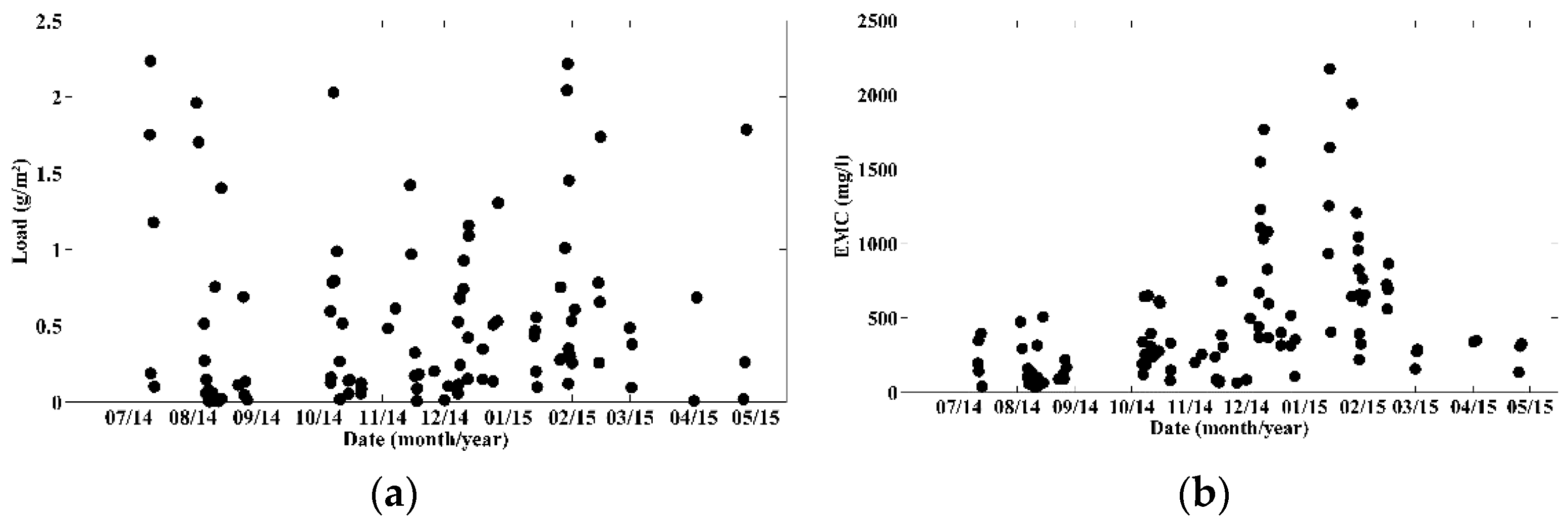
3.1. TSS Concentrations and Loads

Event mean concentration (EMC) is commonly used to evaluate the quality of runoff generated during a wet event and is considered as a surrogate indicator of runoff pollution [38,39]. From the EMC values summarized in

Table 5. Characteristics of TSS EMC and Loads for the monitored events.

Parameter	Maximum	Minimum	Mean	Median	Standard Deviation
EMC (mg/L)	2174.37	35.39	452.09	320.97	432.42
Load (g/m2)	2.23	0.0035	0.51	0.27	0.56

, significant pollutant loads to receiving outlets are noticed. Median EMC of TSS obtained for this site is relatively much higher (320.97 mg/L) than those reported earlier in the literature. Gromaire [2] reported a median EMC of 97 mg/L calculated on six urban roads in “Le Marais” catchment while Gnecco et al. [40] calculated a median EMC equal to 119 mg/L in the experimental catchment of Villa Cambiosa in Italy.

The high EMC from the present study is explained mainly by the site’s characteristics related to high traffic density (~30,000 vehicles per day), since much lower concentrations (median EMC = 66 mg/L) yielded from road catchments that were less frequented [3].

Loads are expressed per unit of area and range from 0.0035 g/m² to 2.23 g/m². The total annual load is equal to 89.23 g/m².

To better understand the variability of EMC and loads of TSS between various storms and seasons, temporal variations are plotted (Figure 3) and seasonal average EMC and total loads are examined (

Table 6. Seasonal values of average EMC (mg/L) and total yields(g/m²) and min-max values of maximum rainfall intensity (mm/h) and rainfall depth (mm) and total rainfall depth of storm events for each season.

Season	Autumn	Winter	Spring	Summer
Beginning date	6 October 2014 15:30	24 December 2014 15:30	01 April 2015 02:53	11 July 2014 02:16
End date	19 December 2014 13:53	2 March 2015 01:13	26 April 2015 12:56	27 August 2014 07:02
Number of events	42	29	5	30
Average EMC (mg/L)	270.35	550.82	326.43	228.37
Total load (g/m2)	18.75	18.83	2.75	13.62
Maximum intensity (mm/h) (min–max)	0.54–72	0.71–72	4.23–120	1.77–180
Rainfall depth (mm) (min–max)	0.2–14.2	0.3–7.8	0.3–6.8	0.4–21.3
Total rainfall depth (mm)	131.3	43.7	11.3	129.2

). A seasonal trend is observed for EMC where the highest values are those recorded during the winter season. The average EMC calculated on winter (550 mg/L) is significantly higher than that on summer (228 mg/L) although the latter’s events are heavier in terms of both precipitation depth and intensity than the former’s. This highlights a dilution effect due to an increase in runoff volume (driven by depth) stronger than the increase in eroded mass (driven by intensity). Indeed, negative Pearson correlation calculated between the average seasonal EMC and the total rainfall depth collected for each season (R = −0.6) support the occurrence of dilution. A similar pattern is not detected for loads whose values are at wide ranges. The seasonal trend disappears in winter and seasonal differences are not easily detected.

Correlation coefficients are calculated between EMC and loads of TSS and rainfall characteristics to identify explanatory variables that may be used to predict EMC and loads. The rainfall characteristics are: antecedent dry weather period (ADWP), storm duration (Duration), average intensity (Imean), maximum intensity (Imax), maximum five-minute intensity (Imax 5) and precipitation amount (Hrain). Pearson correlation coefficients obtained are presented in

Table 7. Pearson correlation coefficients R between EMC and loads of TSS and rainfall characteristics.

Rainfall Characteristic	Pearson Correlation Coefficient R
	TSS	TSS Loads
ADWP	−0.048	0.14
Duration	−0.17	0.37
Imean	−0.19	0.12
Imax	−0.2	0.22
Imax 5	−0.18	0.28
Hrain	−0.26	0.52

.

No correlation is found between EMC and the antecedent dry weather period, which seems to have no effect on runoff quality (R = −0.048). EMC is weakly negatively correlated with the rainfall depth (R = −0.26) and the rainfall duration (R = −0.17) suggesting the occurrence of dilution during long or heavy storm events.

As for loads, significant positive correlations are more common than for EMC. The strongest correlations are with the precipitation depth (R = 0.52) and the storm duration (R = 0.37). Positive correlations are also shown with maximum 5 min rainfall intensity and maximum intensity, but the coefficients are small, equal to 0.28 and 0.22, respectively. TSS loads are also positively correlated with the ADWP, however the correlation is weak as Pearson coefficient is low (R = 0.14).

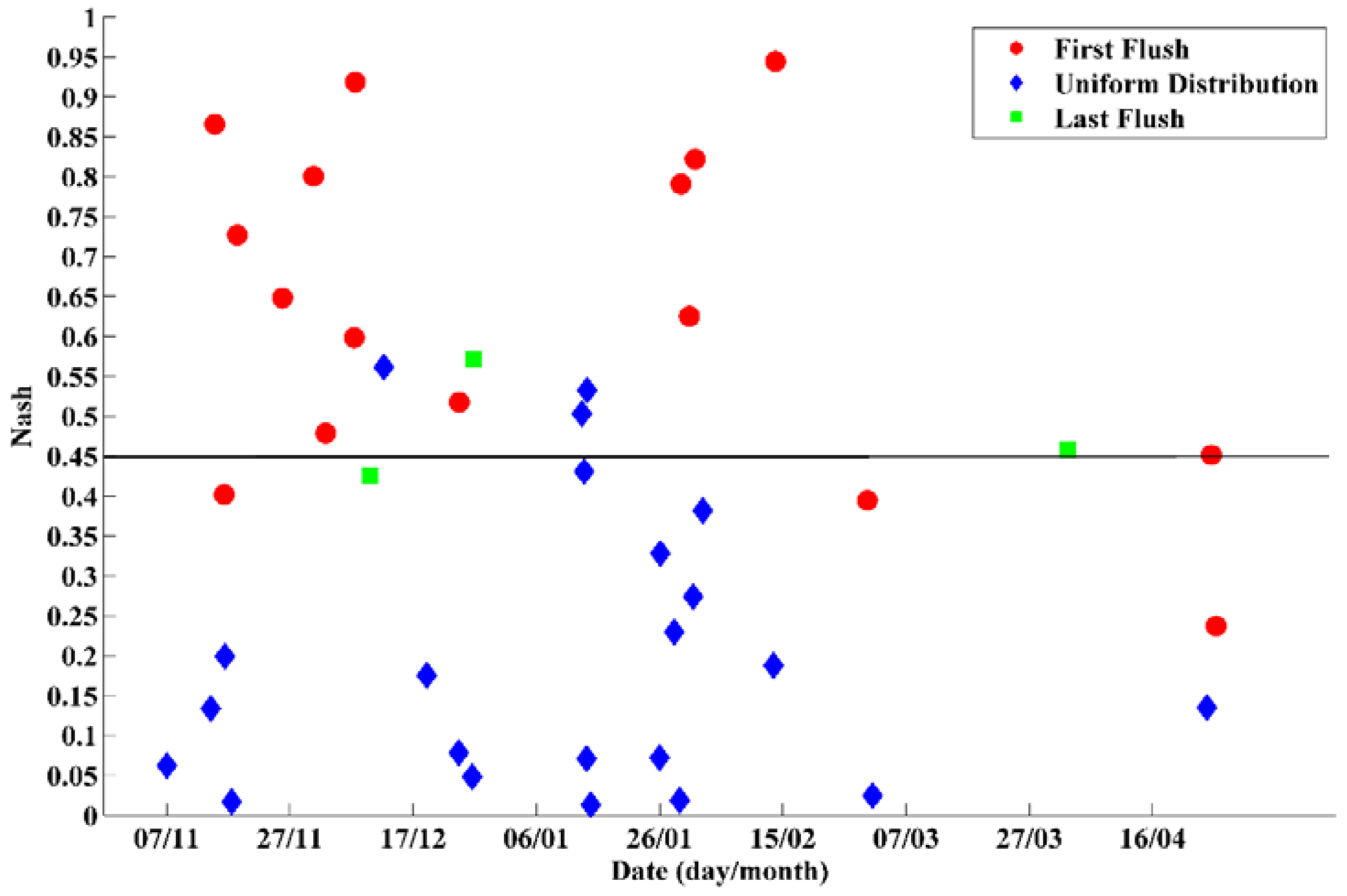
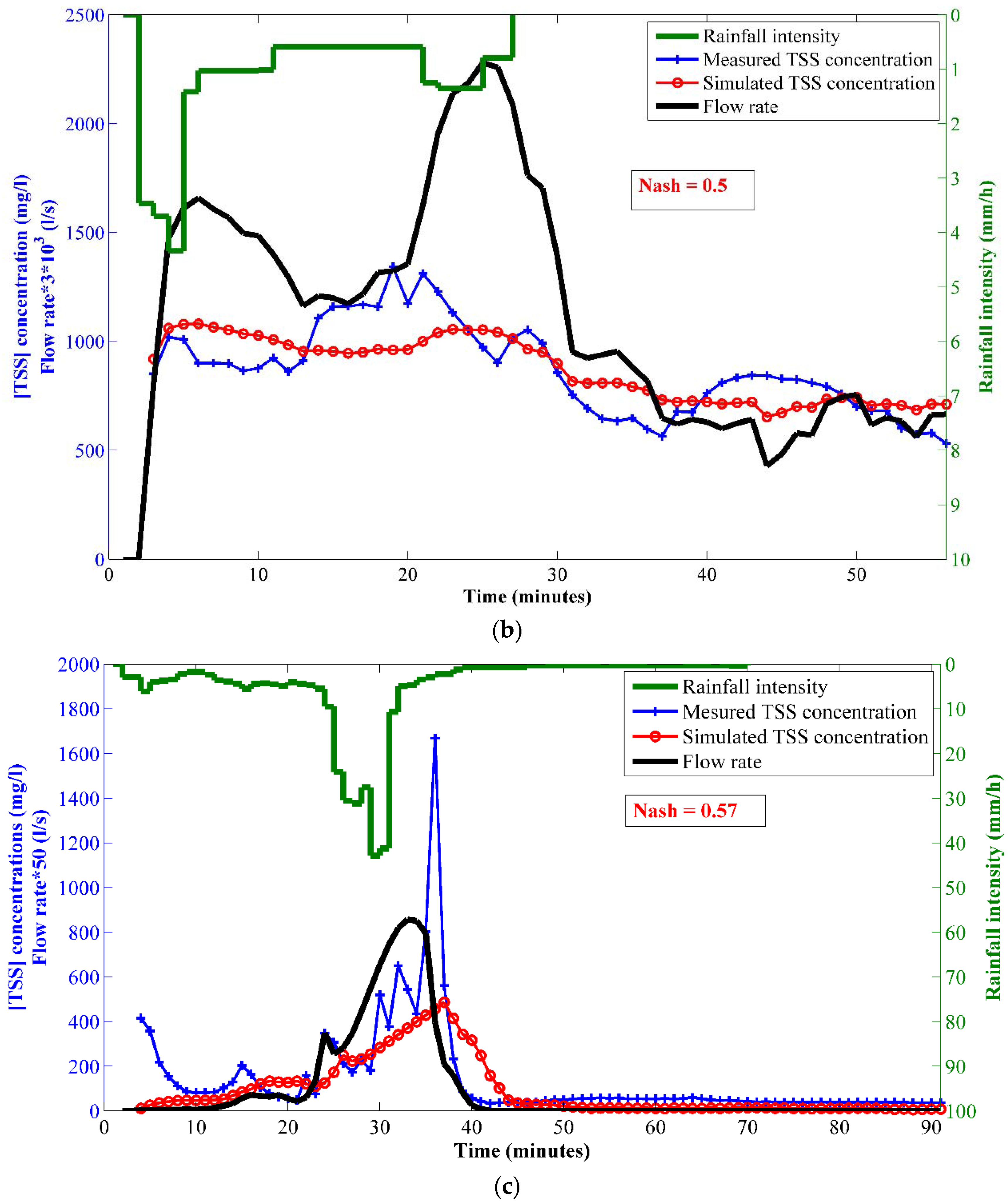
3.2. Dynamic of Transport of TSS

Cumulative mass of TSS plotted against the corresponding cumulative runoff volume is presented in Figure 4. Overall, 17 events are classified as first flush while 22 events are uniformly distributed and three events are last flush.

Clear relationships between M (V) curves and the characteristics of rainfall events are not obvious. Rainfall depth and intensity have no direct influence on the distribution of M (V) curves, and neither does the position of the intensity peak.

3.3. Modeling

In this study we did not intend to replicate pollutant masses and our main concern was to replicate the dynamic of concentrations because several studies have shown that pollutant masses are easily predictable. A recent study by Sage et al. [25], who investigated the capacity of the commonly used accumulation/wash-off models on a similar road catchment, clearly demonstrated that load estimates are accurately replicated by the model with a Nash–Sutcliffe coefficient of 0.79. In addition, their results also show that loads are accurately estimated even with simple EMC models (Nash = 0.77). In fact, as the runoff volume is the main driver of event loads, respectable results are expected when the runoff volume is accurately predicted, therefore achieving high performance for modeling loads is easier than modeling pollutant concentrations and their dynamics which is much more complicated

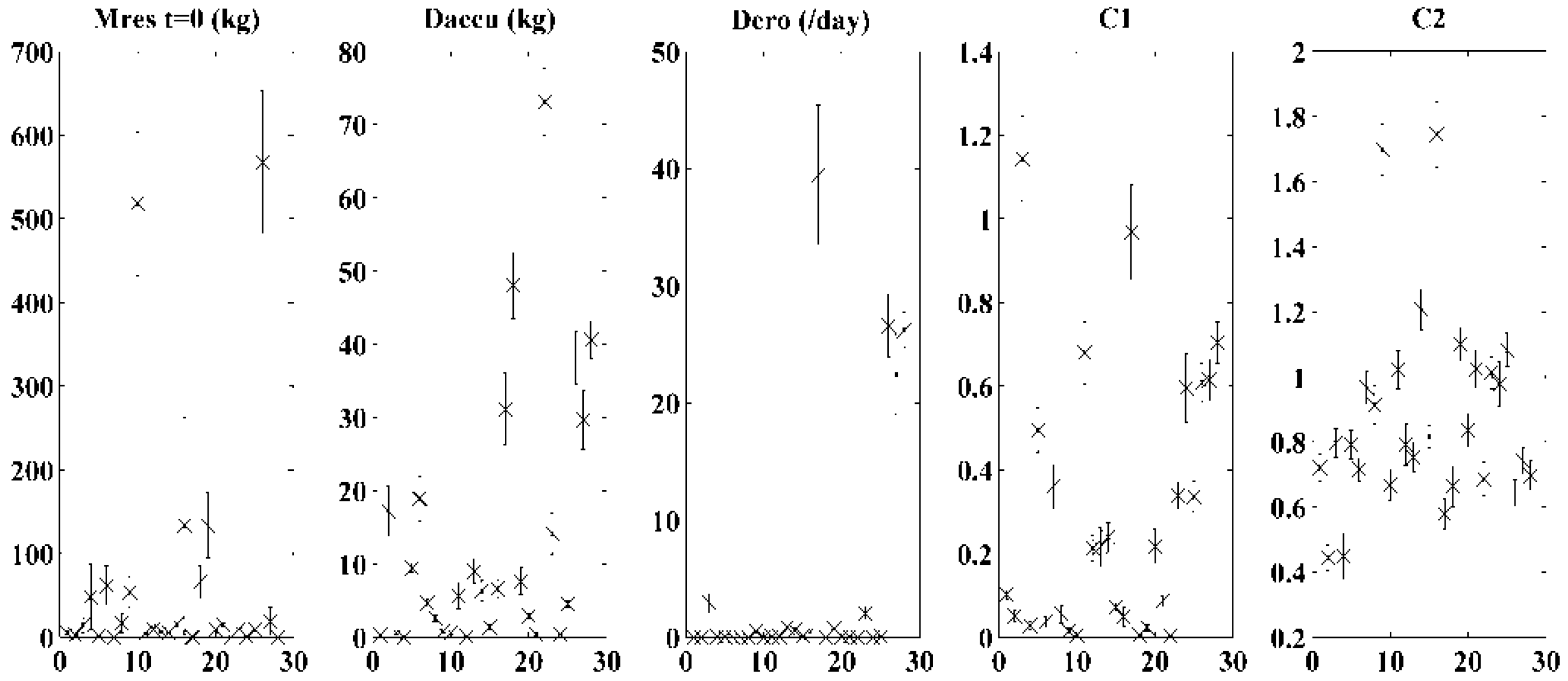
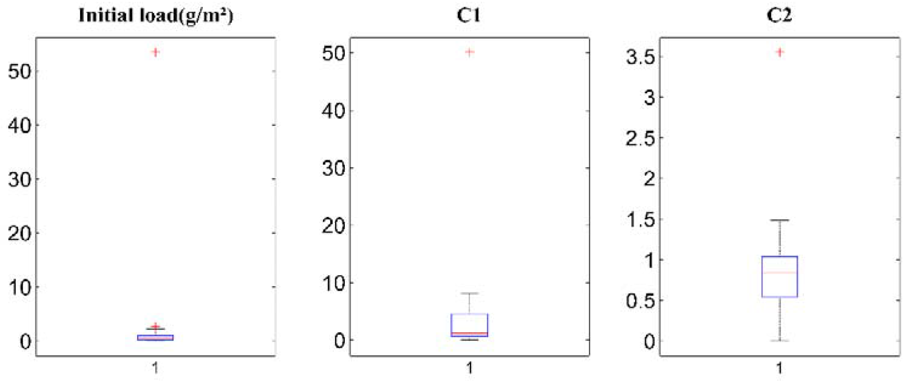
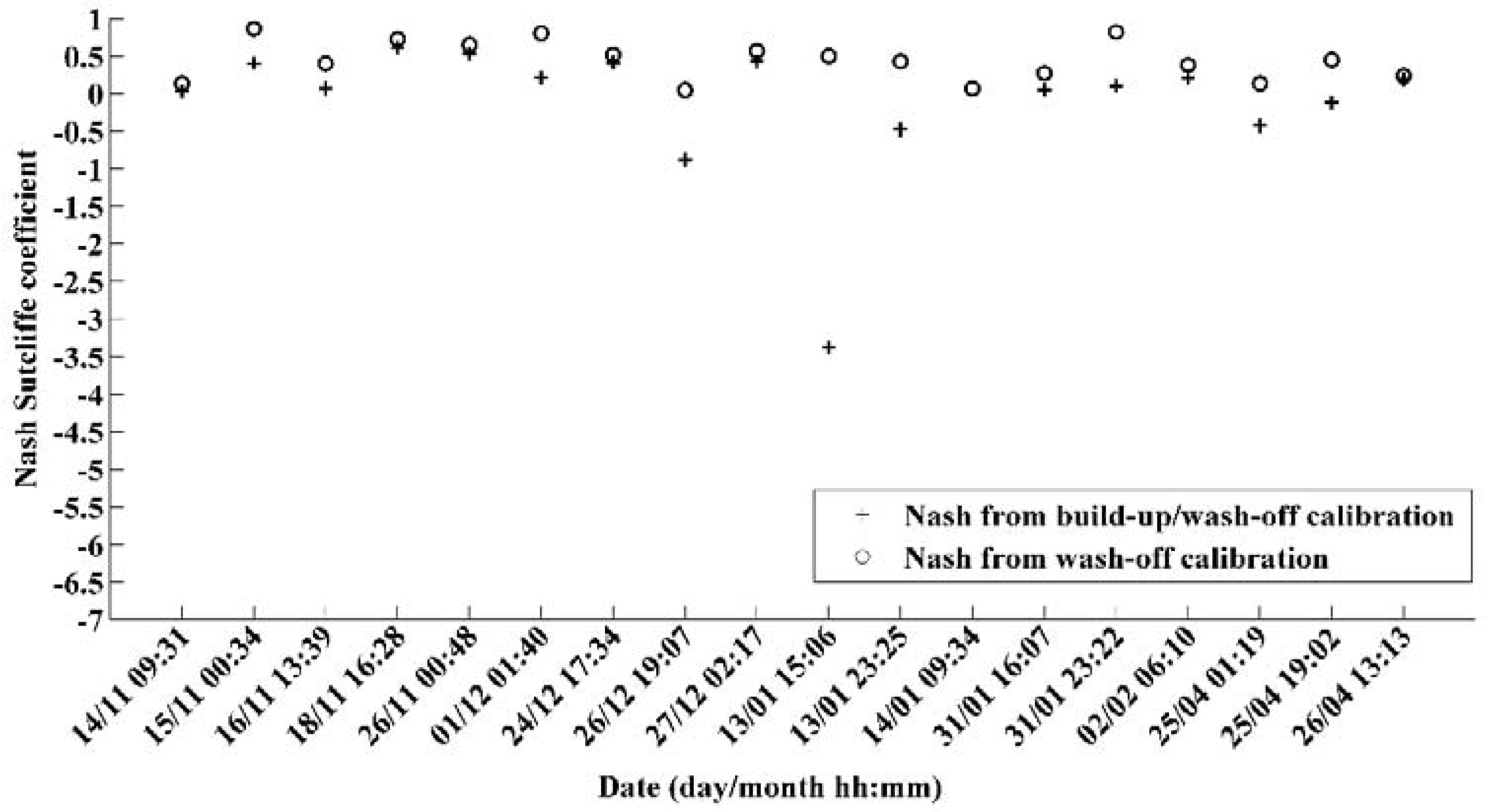
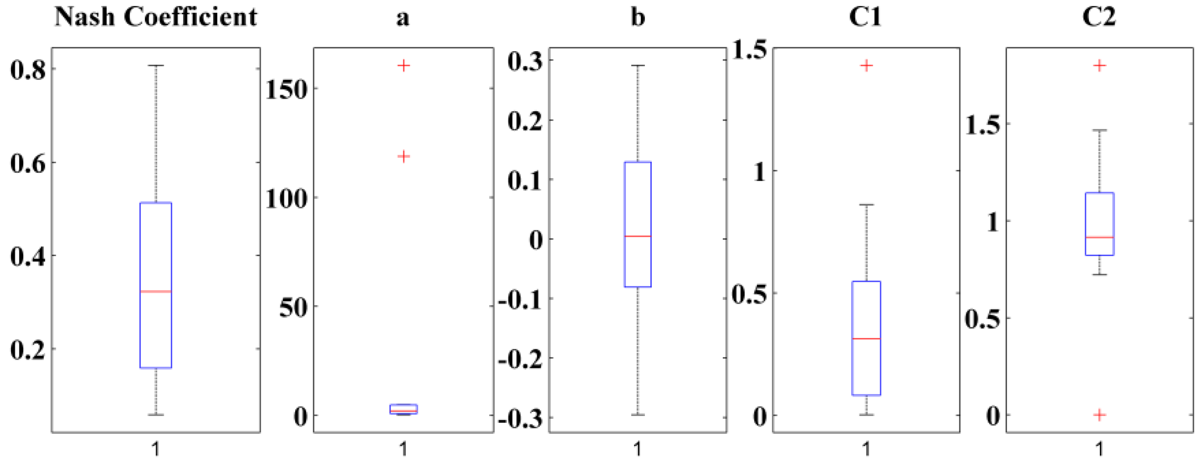
3.3.1. Wash-Off Assessment

Figure 5 illustrates the variation of Nash–Sutcliffe coefficients obtained from calibrating on the whole data set. The best performance of the model is obtained when calibrating on first flush events, where Nash–Sutcliffe efficiency is higher than 0.45 for 14 out of 17 events. This result suggests that the SWWM wash-off model is more suitable for describing the fluctuation of TSS concentrations for first flush events.

For last flush and uniformly distributed events, agreement between measured and simulated TSS concentrations is poor and the model performance is unsatisfactory.

Nash–Sutcliffe coefficients recorded when calibrating over uniformly distributed storms are lower than 0.15 for half of the events. Better results are obtained for last flush events; nevertheless, they are only assessed over three events and Nash–Sutcliffe coefficients are between 0.42 and 0.57.

The pollutographs of three storm events are plotted in Figure 6. It is clearly shown that the simulated data fit very well with the measured data for the first flush event. The dynamic in this case is fully replicated by the model. However, for the other two events, the simulations cannot totally cope with the fluctuations of the concentrations, thus reflecting a lower performance of the model for uniformly distributed and last flush events.

The best replication of TSS concentrations noticed only for first flush events could be attributed to a weakness in the model structure that is not adequate to replicate all types of events and require thus a re-adaptation in order to be not limited to a specific type of events. The re-adaptation could be the coupling of runoff rate with other variables, such as the rainfall intensity, which is proven to be an important explanatory variable of the wash-off process [16], or adding other parameters to the formulation that takes into account the impacts of factors such as the rainfall drop energy and the shear stress.

Since the model performance is not satisfying for all events, the assessment of the variability of optimal parameters as well as the correlations with rainfall characteristics and temperature are performed only on 19 events having a Nash–Sutcliffe coefficient higher than 0.45.

As we can see in Figure 7, showing the boxplots of the calibrated parameters, large variability is observed mainly for the initial load and the wash-off coefficient C1. The calibration on some events also tends to converge to optimum values that have no clear physical significance and that diverge extremely from the mean. The empirical based formulation of SWMM wash-off model may be an explanatory factor of this result. In fact, the variability of the initial available mass prior to a storm event is also noticed on site where dust collection campaigns were carried over three distinct locations. The experimental protocol for dust collection is detailed in Becher et al. [41]. Dust was collected from the gutter, sidewalk and pavement. The highest mass was collected in the gutter with a mean value of 13.76 g/m² compared to 4.14 g/m² and 12.03 g/m² collected, respectively, on the pavement and on the sidewalk. Comparison of the mean observed and simulated values of available load on the surface shows that the simulations (3.53 g/m²) vary in the lower range of observations, which indicates the tendency of the model to underestimate pollutant loads. Moreover, this is confirmed by a significant negative Spearman correlation calculated between the initial load and C1 (R = −0.85, p-value < 0.0001). This correlation [42], which is a Pearson correlation calculated between the ranks of the corresponding variables and is not limited to a linear relation, shows that C1 and the initial load compensate each other which may also explain the difficulties encountered during calibration.

As for the wash-off exponent, the variability in C2 values suggests different patterns of erosion since the wash-off exponent is regarded as an indicator of the shape of the pollutograph [4]. For one event, C2 is calibrated to zero, suggesting linear variation between the washed pollutant mass and the available one for erosion. While for other events, calibrated C2 values are lower than 1 indicating a reduction in the flow rate and therefore slower rate of transport and decreasing of pollutant concentrations from initial values. A recent study by Wijesisri et al. [43] shows that the wash-off of particles less than 150 µm is associated with higher values of wash-off exponent and occurs faster than the wash-off of particles larger than 150 µm. Subsequently, the variation of C2 values maybe also related to the difference in size distribution of the eroded particles.

Correlations for each parameter are summarized in Appendix A (

Table A1. Pearson and Spearman Correlations and their corresponding p-values.

Initial Available Mass
Parameters	R Linear	p-Value	R Spearman	p-Value
Hrain	−0.052	0.836	0.101	0.689
Imax	0.086	0.734	−0.180	0.471
Imax 5	0.122	0.628	−0.015	0.954
Imean	−0.056	0.824	0.032	0.901
Duration	−0.106	0.675	0.120	0.632
ADWP	−0.083	0.742	−0.358	0.144
Tmax	0.509	0.031	0.106	0.674
Tmin	0.436	0.07	0.202	0.420
Tmean	0.491	0.038	0.16	0.525
C1
Parameters	R Linear	p-Value	R Spearman	p-Value
Hrain	−0.184	0.463	−0.597	0.008
Imax	−0.034	0.890	−0.275	0.267
Imax 5	0.009	0.971	−0.257	0.302
Imean	0.779	<0.001	0.153	0.541
Duration	−0.283	0.256	−0.645	0.004
ADWP	0.212	0.398	0.279	0.260
Tmax	0.192	0.445	−0.240	0.336
Tmin	−0.051	0.838	−0.297	0.230
Tmean	0.097	0.701	−0.244	0.327
C2
Parameters	R Linear	p-Value	R Spearman	p-Value
Hrain	0.241	0.321	0.186	0.444
Imax	0.649	0.002	0.368	0.121
Imax 5	0.846	<0.001	0.340	0.154
Imean	0.382	0.106	0.431	0.066
Duration	−0.114	0.642	−0.184	0.448
ADWP	−0.035	0.886	0.098	0.688
Tmax	0.237	0.327	0.136	0.578
Tmin	−0.055	0.823	−0.063	0.797
Tmean	0.067	0.785	0.053	0.827

) and significant correlations are presented in bold.

For the initial available mass, positive linear correlations are only calculated with maximum and average temperature (R_Tmax = 0.509, p-value < 0.031; R_Tmean = 0.49, p-value < 0.038). No correlation exists with the antecedent dry weather period. This could be related to the fact that calibrated mass included other sources of supply such as the residual mass from the previous storm. Past research has shown that a storm event washes only a fraction of the available pollutants [10,33], therefore remaining loads are added to the ones that build-up during dry period between two rainfalls to give the total available mass for wash-off.

As for wash-off coefficient C1 and wash-off exponent C2, significant linear correlations are calculated with average intensity (R_Imean = 0.78, p-value < 0.001) and maximum five-minute intensity (R_Imax = 0.84, p-value < 0.001). This finding is consistent with what we mentioned previously on rapid erosion of pollutants related to higher values of wash-off exponent. Accordingly, it is known that intense rainfalls generate drops with high kinetic energies; therefore, during intense storm events, particles are easily detached, eroded and transported by the flow. Alternatively, rainfalls characterized with low intensities generate a diluted runoff since the runoff transport capacity is weak.

Negative Spearman correlations are calculated between C1 and the rainfall depths (R_rank,Hrain = −0.59, p-value = 0.008) and durations (R_{rank,Duration} = −0.64, p-value = 0.004) respectively; this is likely due to the formulation of the average rainfall intensity that includes the ratio of rainfall depth to rainfall duration.

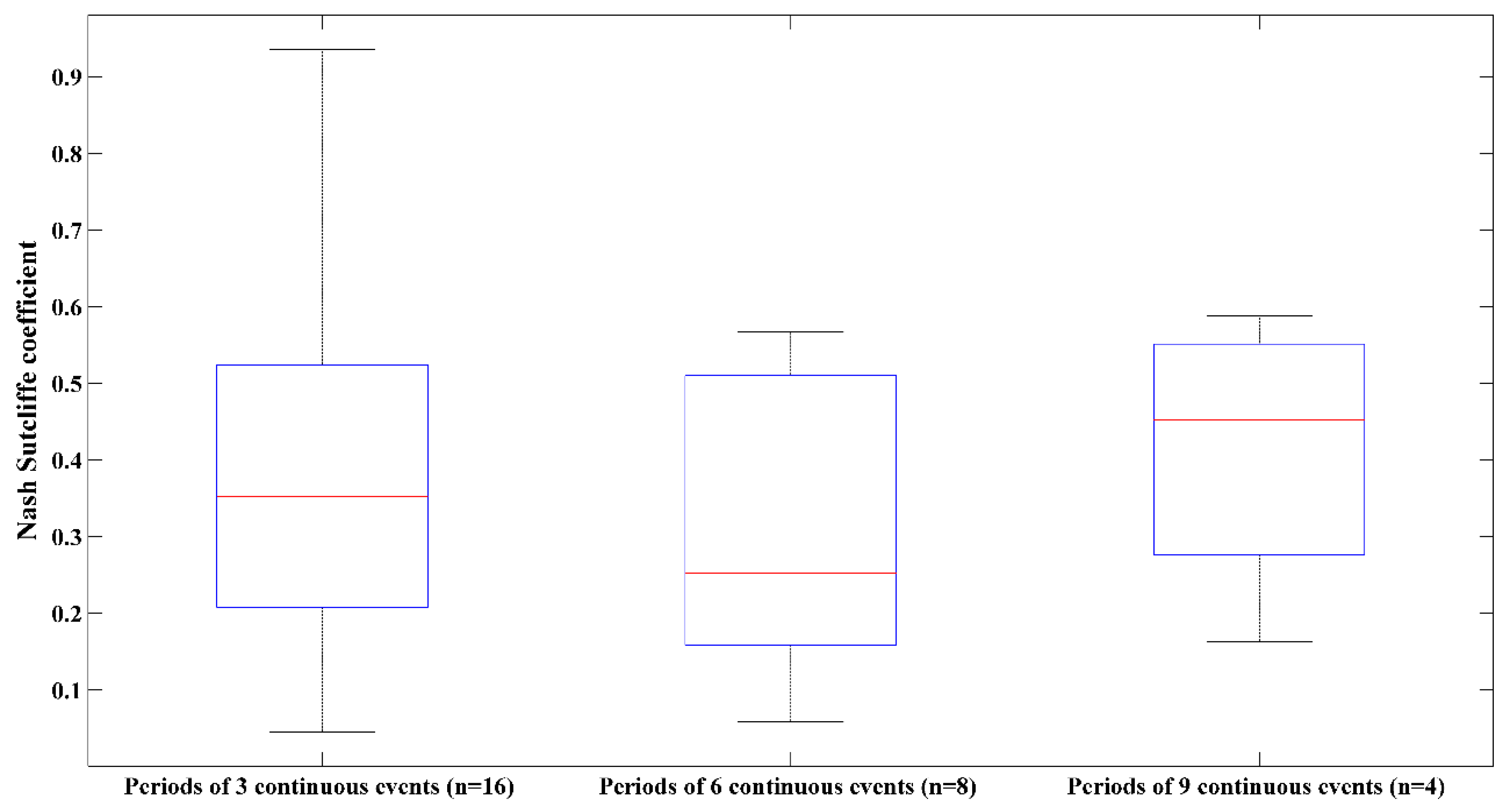
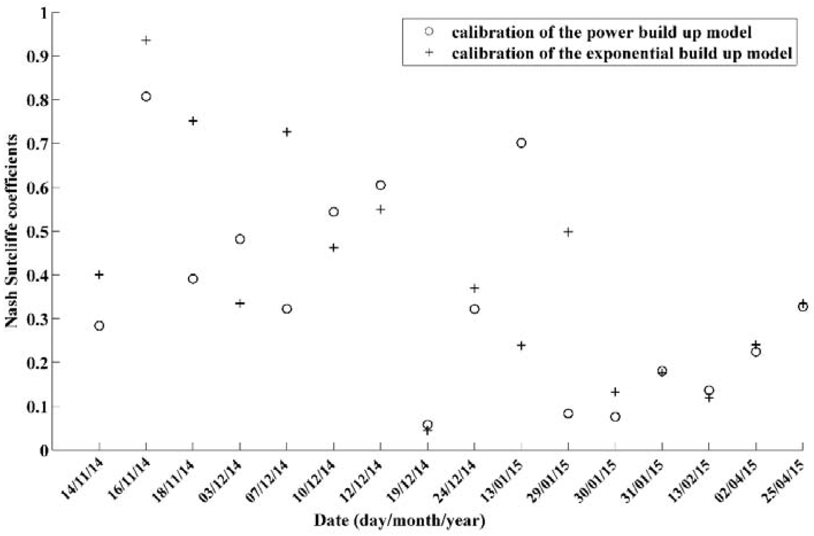
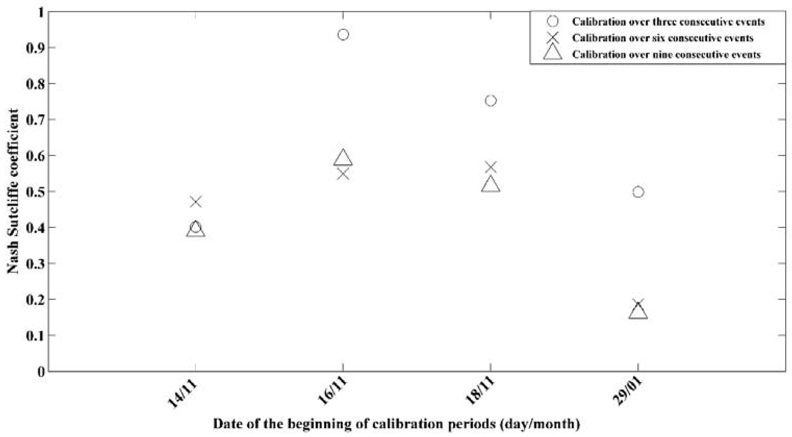
3.3.2. Build-Up Assessment

Calibration results obtained for the tested configurations are presented below.

• Modified SWMM exponential build-up:

Calibrations over periods consisting of three, six and nine continuous events resulted in a wide range of Nash–Sutcliffe coefficients and parameters. Figure 8 shows the boxplot for the Nash–Sutcliffe coefficients obtained for the three periods of calibration.

When calibrating over three events, Nash values vary between 0.045 and 0.93. Half of the periods have a Nash–Sutcliffe efficiency lower than 0.35, suggesting that the fit between the observations and the simulations of TSS concentrations is relatively poor.

Results obtained when calibrating over periods of six events are not more encouraging where the overall variation of Nash–Sutcliffe efficiency is between 0.058 and 0.55.

Calibration over periods of nine continuous events was not possible except for four periods due to missing data. Agreement between the measured and the simulated TSS concentrations is roughly reasonable for one period where the Nash–Sutcliffe coefficient is 0.58, while for the other periods it ranges from 0.16 to 0.51.

The behavior of the build-up model is not very obvious because of the large variability of the obtained Nash–Sutcliffe coefficients and the performance of the model is highly dependent on the calibration period. The variability is also noticed in the optimal sets of calibrated parameters. As seen in Figure 9, the initial available load at the surface has a wide range of variability from zero up to 213.32 g/m². This supports the high stochasticity influencing the accumulation process. The build-up parameters also are at wider ranges than the wash-off coefficients. The accumulation rate represented by the parameter D_accu varies between 0.0075 g/m² and 27.47 g/m², and shows that pollutant accumulation on the surface can be significant for some events. D_ero, the pollutant removal rate during dry weather, is calibrated to zero for most of the events, which indicates that the equilibrium load represented by D_accu/D_ero tends to infinity, supporting the hypothesis of the presence of unlimited supply on the surface. As for wash-off coefficients, C1 has broader interval of variation than C2 who appears to be the best determined parameter since it fluctuates in the interval between 0.6 and 0.8 for the majority of the events. The uncertainty on the estimated parameters seems to be insignificant except for some events where the high dispersion of the calibrated parameter indicate that the model is not sensitive to the best calibrated set of parameters and that no optimum truly exist. This uncertainty will induce errors in the modeling outputs and justifies the low Nash–Sutcliffe efficiencies obtained is some cases.

To evaluate the suitability of the model for simulating the TSS concentrations over long term, we decided to calibrate the model over four successive incrementing length periods of three events increment and then compare the obtained Nash–Sutcliffe efficiencies.

As indicated in Figure 10 the model capacity to estimate the accumulated load between storm events has clearly declined after considering more than 3 events except for the first calibration period that started on the 14 November. For example, Nash coefficient has decreased from 0.93, to 0.54 and 0.58, respectively, when the calibration period starting the 16 November is extended to include six and nine consecutive events. The model performance is slightly different when comparing calibrations over six and nine events, with better Nash–Sutcliffe efficiency calculated over the periods consisting of six events except for the 16 November. This finding reveals the difficulties of calibrating the build-up model and the inefficiency of the model as it is to reproduce the inter-event variability and the complexity of the accumulation process over a long temporal scale.

Further investigation consisted on comparing the results obtained under the assumption of exponential build-up and the results obtained when the build-up model was omitted. Nash–Sutcliffe efficiencies are calculated in each case and the results are summarized in Figure 11.

The comparison shows that the model performance has decreased when the build-up model is introduced, suggesting that the initial TSS load predicted by the model is incorrect. Acceptable results were only obtained for the calibration period starting on the 18 November where the Nash–Sutcliffe coefficients calculated when calibrating the build-up (0.614 and 0.529) were slightly different from the Nash–Sutcliffe coefficients calculated when calibrating only the wash-off (0.727 and 0.648). However, for the rest of calibration periods, the ability to replicate TSS concentrations clearly decreased. This result indicates that the model performance is not significantly affected by modeling the pollutant build-up, which can be easily neglected without any consequences on the predictive capacity of the model.

• Power build-up:

Calibration of the model is first performed over 16 periods of three consecutive events each. Same as for the exponential model, the model performance and the calibrated parameters are very distinct from one event to another as shown in Figure 12.

Nash–Sutcliffe coefficients range between 0.058 and 0.8 and the values associated with build-up parameters a and b are extremely variable. This is related mainly to the existing correlation between these parameters (R_Pearson = −0.56, p-value = 0.023), indicating that same results can be obtained combining different sets of a and b. The calibration of the parameter b results in negative and low values for most of the periods which proves that the model is completely dependent on the coefficient a to better fit the observations and that is not using the antecedent dry weather period as a predictive variable. Parameter a have the biggest weight in the calibration of the model and it compensates the effect of all other component. These results indicate that the structure of the model should be reviewed.

Comparison between the performances of the exponential and the power equations reveals that no specific model has the best performance for all periods (Figure 13). It seems that the exponential model outperforms the power model when calibrated on periods before 30 January and after that date the two models perform similarly in terms of simulating TSS concentrations.

The replication of the variability of the accumulation process under the assumption of dry weather period as being the main explanatory variable does not seem very accurate. The test of both SWMM and power models based on dry weather period and their unsatisfactory performance support this assumption.

Different sources of supply independent of dry weather period and resulting from random phenomenon such as leaf fall, and de-icing salt during fall and winter as well as animal wastes that occur between events are not taken into consideration in the models in their current formulation, which highly affect the stock of mass present of the surface and lead to a failure in its accurate estimate.

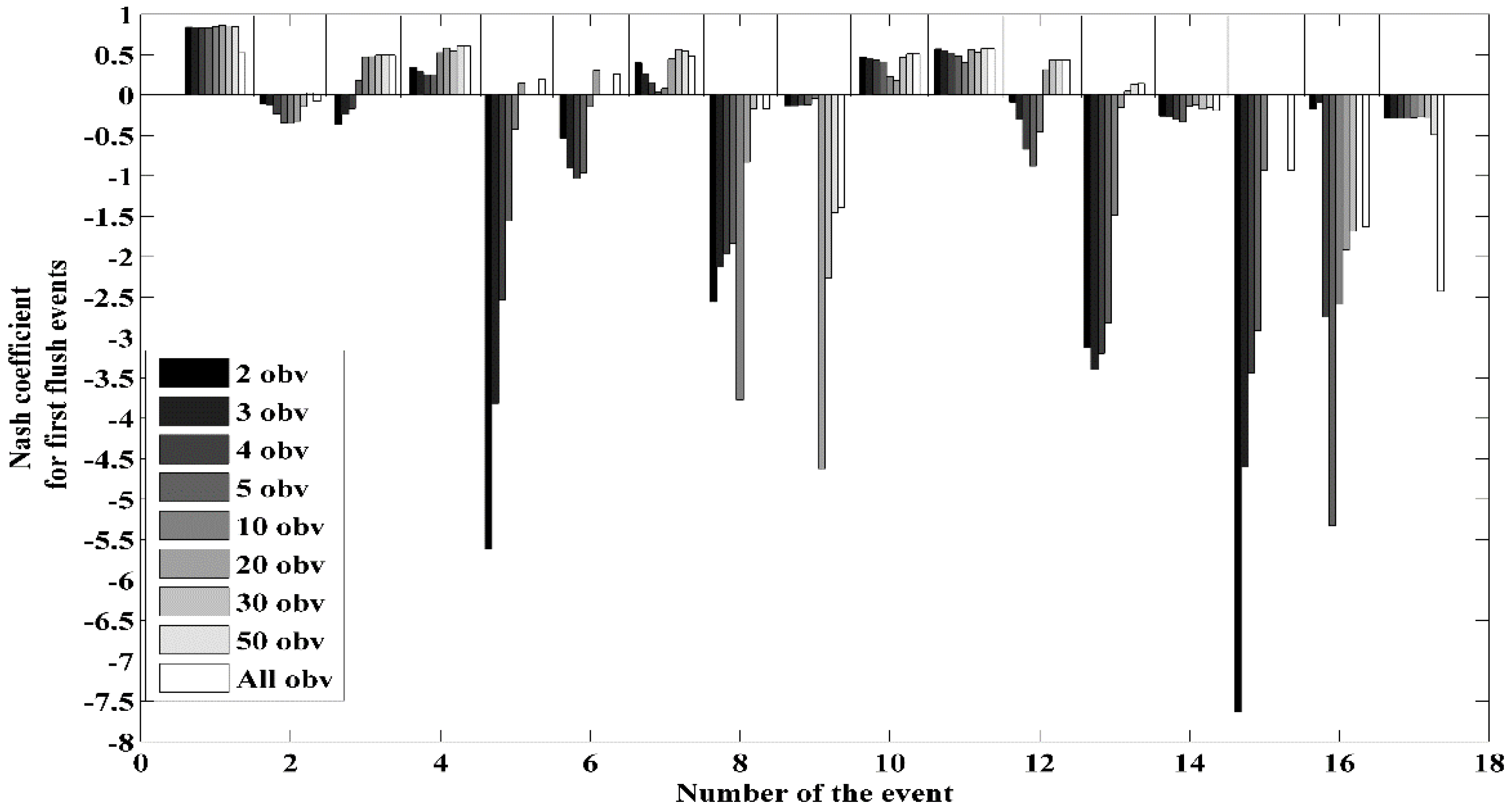
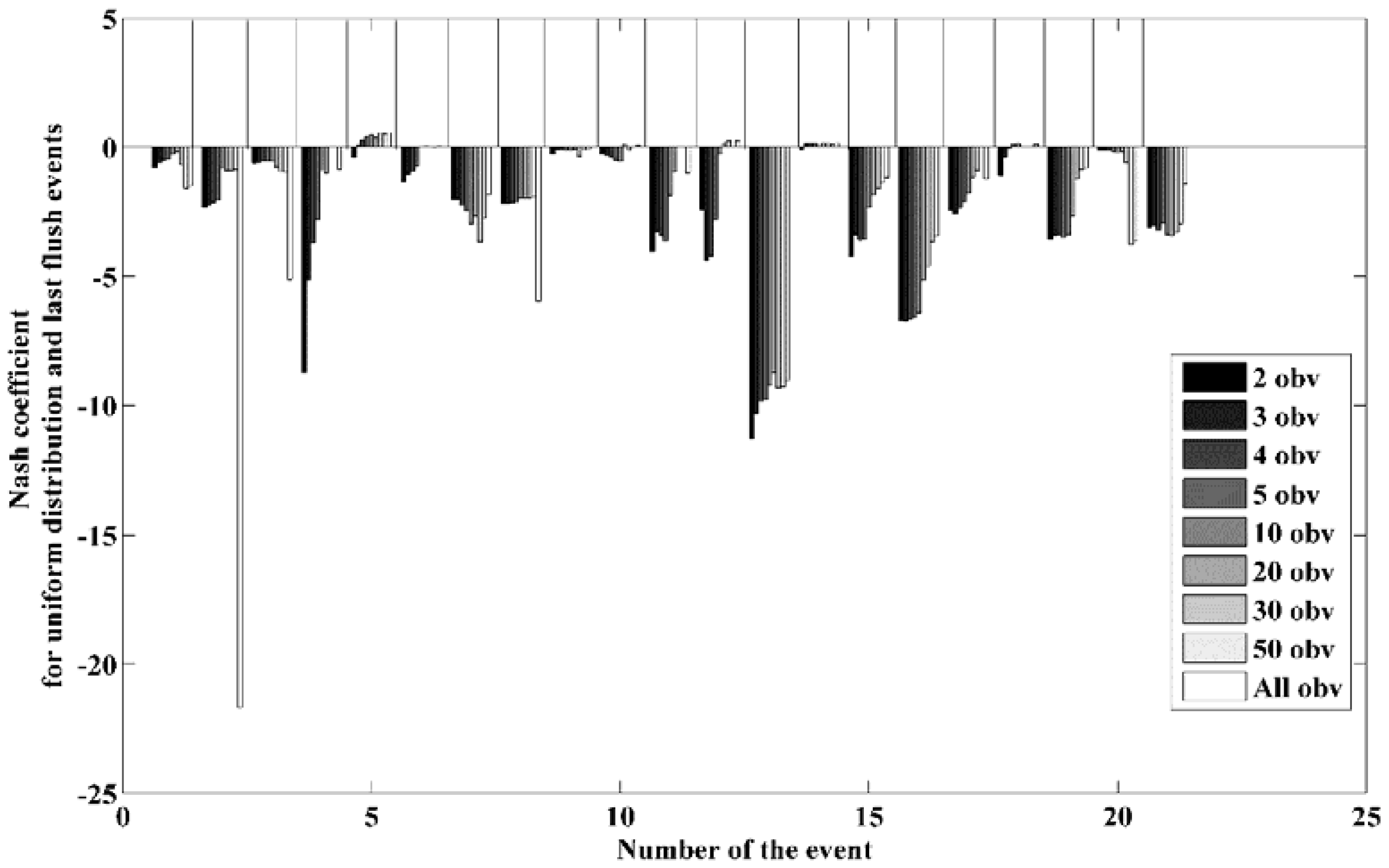
3.3.3. Short Term Predictive Capacity

To assess the short term predictive capacity of water quality model that couples the exponential build-up and SWMM wash-off equations, two methodologies are tested and the obtained results are presented in the sections below.

• Inter-Event:

The first approach consists of validating the model on the events immediately after the calibration period, making the assumption that the parameters remain valid during a given time after calibration. Only periods for which calibration was successful were considered. The results show that despite the efficient calibration of the model, its prediction capacity is very poor (

Table 8. Nash Coefficients obtained from calibration and validation over the modelling period.

Beginning of the Modeling Period	Nash Coefficient from Calibration over the First Two Events	Nash Coefficient from Validation over the Third Event
14 November 2014	0.527	−0.5714
17 November 2014	0.787	−0.5981
7 December 2014	0.781	0.1643
13 January 2015	0.616	−0.5890
30 January 2015	0.629	−0.8874

).

The Nash–Sutcliffe coefficients reflect a very weak replication of the pollutograph and show that high errors are included in the predicted TSS concentrations, which do not seem to fit at all the observations and are very far from the ranges of variations of the measurements. The application of such models to predict pollutants from storm water runoff is thus largely limited and suggest that the characteristics of the calibrated parameters certainly cannot be kept or extended even to a limited number of events following immediately calibration period, making the assumption that calibrated parameters are not site specific rather event specific and that no unique set of parameters can replicate accurately the pollutographs for all considered periods.

• Intra-Event:

This approach consists in calculating the available pollutant mass at the beginning of the storm using the measurements recorded on the first time steps and the wash-off parameters calibrated from a previous knowledge of the studied site. The method is assessed over 38 single events. Four events are excluded because their calibration efficiency is very low. The 38 events consist of 17 first flush events, 18 with uniform distribution of pollutants and three last flush.

The calculated Nash–Sutcliffe Coefficients over the 38 events are presented in the Figure 14 and Figure 15 below. The bar plots distinguish the results in function of the number of points considered for the calculation of the available initial load for erosion.

Validation results are mostly satisfactory when applying this method over first flush events. Three events are accurately predicted when using only the first two observations for calculating the available erodible load where Nash–Sutcliffe efficiencies were equal to 0.83, 0.57 and 0.46. Based on the first 30 points of observations, the model adequately predicted six events. This is an interesting result and could be helpful for the operational in the context of predicting the dynamic of the pollutants during a rainfall event only by knowing the dynamic at the beginning of the storm.

As for the uniformly distributed events and the last flush events, the prediction of the model is not satisfying except for one uniform event where the pollutant concentrations are predicted with a Nash–Sutcliffe efficiency equal to 0.43, calculated when five points of the observations were included in the estimation of the available mass and it increased to 0.54 if the first 30 min of measurements were considered.

The intra-event approach based on data assimilation seems to be promising and deserves further investigation so it can be extended to give accurate prediction not only to first flush events. The interest of this approach is that it may help planners and engineers to make accurate loading estimates based only on the first measurements and on the knowledge of the behavior of the catchment. Monitoring devices can be thus implemented to record the first points of observations, which can be transmitted automatically to a registration system and be integrated directly with numerical simulations.

4. Conclusions and Perspectives

This study presents a framework on modeling and assessing the TSS concentration generated during storm events on an urban road catchment. Qualitative characterization of the studied site as well as calibration and prediction assessment of different water quality configurations are performed on a long-term data base collected between June 2014 and April 2015. The results show that the performance of SWMM wash-off model depends on the dynamic of transport of pollutant during the event where the best fit between the observed and simulated TSS concentrations is recorded for first flush events. Assessment of SWMM exponential build-up model reveals that the model performs better on short periods suggesting the incapacity of the model to simulate the variation of the available mass for erosion for long periods. High variability involved in modeling the production of pollutants emerges from the large differences in the model’s performance over distinct calibration periods. This behavior must be further investigated and stochastic approaches might hold the answers to better understand the accumulation process [43,44,45]. As for the predictive capacity of the model on the inter-event scale, the results clearly prove the inadequacy of the traditional build-up/wash-off model to predict the pollutograph using calibrated parameters, which seem to be event specific rather than site specific. The complexity of the accumulation and wash-off process, which is not very explicit in the model structure, and the absence of factors that play an important role in the generation of pollutants would have a significant fingerprint on the model outputs. On the intra-event scale, based on data assimilation, the model predicts half of the first flush events but is not able to predict last flush and the uniformly distributed events, which does not seem very surprising since these events were not satisfactorily calibrated. This method is very interesting for management practices because of its simplicity and its easy implementation; in addition, it also resolves the problem of missing data that occurs sometimes due to technical problems, making it possible to estimate the yield of a storm event even if not all points are recorded. Further investigation is indeed necessary to enhance this method and develop further the integration of data assimilation in the water quality modeling.

The complexity of the build-up and the wash-off processes and their limited knowledge in addition to the high variability in the modeling results highlighted in this study, rise the need for further in deep investigation of the mechanisms governing the generation and the transport of pollutant in urban catchments. For that matter, extensive site monitoring is recommended to better understand and assess from a physical point of view the implicated factors in the accumulation and erosion processes and the interactions within the system to have a precise and accurate estimation of the pollutograph generated during wet weather.

References

1. Elliott, A.; Trowsdale, S. A review of models for low impact urban stormwater drainage. Environ. Model. Softw. 2007, 22, 394–405. [Google Scholar] [CrossRef]
2. Gromaire, M.-C. La Pollution des Eaux Pluviales Urbaines en Réseau d’Assainissement Unitaire. Caractéristiques et Origines; Ecole des Ponts ParisTech: Marne-la-Vallée, France, 1998. [Google Scholar]
3. Bressy, A. Flux de Micropolluants Dans les Eaux de Ruissellement Urbaines: Effets de Différents Modes de Gestion à l’Amont; Université Paris-Est: Paris, France, 2010. [Google Scholar]
4. Bai, S.; Li, J. Sediment Wash-Off from an Impervious Urban Land Surface. J. Hydrol. Eng. 2013, 18, 488–498. [Google Scholar] [CrossRef]
5. Gunawardana, C.; Goonetilleke, A.; Egodawatta, P.; Dawes, L.; Kokot, S. Role of Solids in Heavy Metals Buildup on Urban Road Surfaces. J. Environ. Eng. 2012, 138, 490–498. [Google Scholar] [CrossRef] [Green Version]
6. Herngren, L.; Goonetilleke, A.; Ayoko, G.A. Analysis of heavy metals in road-deposited sediments. Anal. Chim. Acta 2006, 571, 270–278. [Google Scholar] [CrossRef] [PubMed] [Green Version]
7. Mahbub, P.; Goonetilleke, A.; Ayoko, G.A.; Egodawatta, P.; Yigitcanlar, T. Analysis of build-up of heavy metals and volatile organics on urban roads in gold coast, Australia. Water Sci. Technol. 2011, 63, 2077–2085. [Google Scholar] [CrossRef] [PubMed] [Green Version]
8. Sabin, L.D.; Lim, J.H.; Stolzenbach, K.D.; Schiff, K.C. Contribution of trace metals from atmospheric deposition to stormwater runoff in a small impervious urban catchment. Water Res. 2005, 39, 3929–3937. [Google Scholar] [CrossRef] [PubMed]
9. Shaw, S.B.; Walter, M.T.; Steenhuis, T.S. A physical model of particulate wash-off from rough impervious surfaces. J. Hydrol. 2006, 327, 618–626. [Google Scholar] [CrossRef]
10. Vaze, J.; Chiew, F.H. Experimental study of pollutant accumulation on an urban road surface. Urban Water 2002, 4, 379–389. [Google Scholar] [CrossRef]
11. Bertrand-Krajewski, J.-L.; Chebbo, G.; Saget, A. Distribution of pollutant mass vs volume in stormwater discharges and the first flush phenomenon. Water Res. 1998, 32, 2341–2356. [Google Scholar] [CrossRef]
12. European Commission. Directive of the European Parliament and of the Council n 2000/60/EC establishing a framework for the community action in the field of water policy. Off. J. Eur. Communities 2000, 327, 1–72. [Google Scholar]
13. Dotto, C.B.S.; Kleidorfer, M.; Deletic, A.; Rauch, W.; McCarthy, D.T.; Fletcher, T.D. Performance and sensitivity analysis of stormwater models using a Bayesian approach and long-term high resolution data. Environ. Model. Softw. 2011, 26, 1225–1239. [Google Scholar] [CrossRef]
14. Sartor, J.D.; Boyd, G.B.; Agardy, F.J. Water Pollution Aspects of Street Surface Contaminants. J. Water Pollut. Control Fed. 1974, 46, 458–467. [Google Scholar] [PubMed]
15. Francey, M.; Duncan, H.P.; Deletic, A.; Fletcher, T.D. Testing and Sensitivity of a Simple Method for Predicting Urban Pollutant Loads. J. Environ. Eng. 2011, 137, 782–789. [Google Scholar] [CrossRef]
16. Vaze, J.; Chiew, F.H.S. Comparative evaluation of urban storm water quality models. Water Resour. Res. 2003, 39, 1280. [Google Scholar] [CrossRef]
17. Alley, W.; Smith, P. Estimation of Accumulation Parameters for Urban Runoff Quality Modeling. Water Resour. Res. 1981, 17, 1657–1664. [Google Scholar] [CrossRef]
18. Heng, B.C.P.; Sander, G.C.; Armstrong, A.; Quinton, J.N.; Chandler, J.H.; Scott, C.F. Modeling the dynamics of soil erosion and size-selective sediment transport over nonuniform topography in flume-scale experiments. Water Resour. Res. 2011, 47. [Google Scholar] [CrossRef] [Green Version]
19. Massoudieh, A.; Abrishamchi, A.; Kayhanian, M. Mathematical modeling of first flush in highway storm runoff using genetic algorithm. Sci. Total Environ. 2008, 398, 107–121. [Google Scholar] [CrossRef] [PubMed]
20. Hong, Y.; Bonhomme, C.; Le, M.-H.; Chebbo, G. A new approach of monitoring and physically-based modelling to investigate urban wash-off process on a road catchment near Paris. Water Res. 2016, 102, 96–108. [Google Scholar] [CrossRef] [PubMed]
21. Ball, J.E.; Jenks, R.; Aubourg, D. An assessment of the availability of pollutant constituents on road surfaces. Sci. Total Environ. 1998, 209, 243–254. [Google Scholar] [CrossRef]
22. Huber, W.C.; Dickinson, R.E.; Barnwell, T.O., Jr.; Branch, A. Storm Water Management Model, Version 4; U.S. Environmental Protection Agency, Environmental Research Laboratory: Athens, GA, USA, 1988.
23. Servat, E. Contribution à l’étude de la Pollution du Ruissellement Pluvial Urbain. Ph.D. Thesis, Université des Sciences et Techniques du Languedoc, Montpellier, France, 1987. [Google Scholar]
24. Dembélé, A.; Bertrand-Krajewski, J.-L.; Becouze, C.; Barillon, B.; Dauthuille, P. TSS, COD and Priority Pollutants in Stormwater—Event Fluxes Modelling Using Conceptual Approach. 2013. Available online: http://hdl.handle.net/2042/51284 (accessed on 7 December 2015).
25. Sage, J.; Bonhomme, C.; Al Ali, S.; Gromaire, M.-C. Performance assessment of a commonly used “accumulation and wash-off” model from long-term continuous road runoff turbidity measurements. Water Res. 2015, 78, 47–59. [Google Scholar] [CrossRef] [PubMed] [Green Version]
26. Wang, L.; Wei, J.; Huang, Y.; Wang, G.; Maqsood, I. Urban nonpoint source pollution buildup and washoff models for simulating storm runoff quality in the Los Angeles County. Environ. Pollut. 2011, 159, 1932–1940. [Google Scholar] [CrossRef] [PubMed]
27. Kanso, A.; Tassin, B.; Chebbo, G. A benchmark methodology for managing uncertainties in urban runoff quality models. Water Sci. Technol. 2005, 51, 163–170. [Google Scholar] [PubMed]
28. Métadier, M.; Bertrand-Krajewski, J.-L. From mess to mass: A methodology for calculating storm event pollutant loads with their uncertainties, from continuous raw data time series. Water Sci. Technol. 2011, 63, 369. [Google Scholar] [CrossRef] [PubMed]
29. Mourad, M.; Bertrand-Krajewski, J.-L. A method for automatic validation of long time series of data in urban hydrology. Water Sci. Technol. 2002, 45, 263–270. [Google Scholar] [PubMed]
30. Becouze-Lareure, C.; Invernon, N. EVOHE-Logiciel de Suivi des Capteurs—Validation de Données-Auto-Surveillance des Systèmes d’Assainissement; INSA Lyon ALISON: Lyon, France, 2014. [Google Scholar]
31. Zoppou, C. Review of urban storm water models. Environ. Model. Softw. 2001, 16, 195–231. [Google Scholar] [CrossRef]
32. Obropta, C.C.; Kardos, J.S. Review of Urban Stormwater Quality Models: Deterministic, Stochastic, and Hybrid Approaches JAWRA. J. Am. Water Resour. Assoc. 2007, 43, 1508–1523. [Google Scholar] [CrossRef]
33. Egodawatta, P.; Thomas, E.; Goonetilleke, A. Mathematical interpretation of pollutant wash-off from urban road surfaces using simulated rainfall. Water Res. 2007, 41, 3025–3031. [Google Scholar] [CrossRef] [PubMed] [Green Version]
34. Egodawatta, P. Translation of Small-Plot Scale Pollutant Build up and Wash off Measurements to Urban Catchment Scale. Ph.D. Thesis, Queensland University of Technology, Brisbane, Australia, 2007. [Google Scholar]
35. Bonhomme, C.; Petrucci, G. Spatial Representation in semi-distributed modelling of water quantity and quality. In International Conference on Urban Drainage, Kuching, Malaysia; ICUD: Kuching, Malaysia, 2014; p. 2488399. [Google Scholar]
36. Hasting, W.K. Monte carlo sampling methods using Markov chains and their applications. Biometrika 1970, 57, 97–109. [Google Scholar] [CrossRef]
37. Nash, J.E.; Sutcliffe, J.V. River flow forecasting through conceptual models part I—A discussion of principles. J. Hydrol. 1970, 10, 282–290. [Google Scholar] [CrossRef]
38. Lee, J.H.; Bang, K.W.; Ketchum, L.H.; Choe, J.S.; Yu, M.J. First flush analysis of urban storm runoff. Sci. Total Environ. 2001, 293, 163–175. [Google Scholar] [CrossRef]
39. Maniquiz, M.C.; Lee, S.; Kim, L.-H. Multiple linear regression models of urban runoff pollutant load and event mean concentration considering rainfall variables. J. Environ. Sci. 2010, 22, 946–952. [Google Scholar] [CrossRef]
40. Gnecco, I.; Berretta, C.; Lanza, L.G.; La Barbera, P. Storm water pollution in the urban environment of Genoa, Italy. Atmos. Res. 2005, 77, 60–73. [Google Scholar] [CrossRef]
41. Bechet, B.; Bonhomme, C.; Lamprea, K.; Campos, E.; Jean Soro, L.; Dubois, P.; Lherm, D. Towards a Modeling of Traffic Pollutant Flux at Local Scale—Chemical Analysis and Micro-Characterization of Road Dusts. Available online: http://hues.se/assets/Abstract_final_2015-05-27-final1.pdf (accessed on 22 March 2016).
42. Spearman, C. The Proof and Measurement of Association between Two Things. Am. J. Psychol. 1904, 15, 72–101. [Google Scholar] [CrossRef]
43. Wijesiri, B.; Egodawatta, P.; McGree, J.; Goonetilleke, A. Influence of pollutant build-up on variability in wash-off from urban road surfaces. Sci. Total Environ. 2015, 527–528, 344–350. [Google Scholar] [CrossRef] [PubMed]
44. Daly, E.; Bach, P.M.; Deletic, A. Stormwater pollutant runoff: A stochastic approach. Adv. Water Resour. 2014, 74, 148–155. [Google Scholar] [CrossRef]
45. Wijesiri, B.; Egodawatta, P.; McGree, J.; Goonetilleke, A. Incorporating process variability into stormwater quality modelling. Sci. Total Environ. 2015, 533, 454–461. [Google Scholar] [CrossRef] [PubMed]
Figure 1. The studied catchment delimited in bold black line. In the image we see the location of the sewer inlet station and the meteorological station insalled at 180 m from the sewer inlet and 15 m of the extremity of the catchment (Photo taken from Google Map@2016).
Water 08 00312 g001
Figure 2. Definition of the M(V) curve zones.
Water 08 00312 g002
Figure 3. (a) Temporal variation of EMC (mg/L) for TSS from June 2014 to April 2015; and (b) temporal variation of load (g/m2) for TSS from June 2014 to April 2015.
Water 08 00312 g003
Figure 4. M (V) of TSS for 42 events from November 2014 to April 2015. The bold lines represent the upper (line with cross) and lower (line with circles) boundaries for the First Flush and Last Flush Zone.
Water 08 00312 g004
Figure 5. Variation of the Nash–Sutcliffe coefficients obtained when calibrating on first flush, uniformly distributed and last flush events.
Water 08 00312 g005
Figure 6. Calibration results for the rainfall events of: (a) 14 February 15 (First flush event); (b) 27 December 14 (Uniformly distributed event); and (c) 13 January 15 (Last flush event).
Water 08 00312 g006aWater 08 00312 g006b
Figure 7. Boxplots of optimal calibrated wash-off parameters. The central mark of each box is the median, the edges represent the 25th and 75th percentiles, and the whiskers extend to the maximum and minimum values that are not considered as outliers.
Water 08 00312 g007
Figure 8. Boxplots of Nash–Sutcliffe coefficients obtained when calibrating over periods of three, six and nine continuous events. The central mark of each box is the median of the Nash coefficients, the edges represent the 25th and 75th percentiles, and the whiskers.
Water 08 00312 g008
Figure 9. Standard deviation of the posterior probability of build-up and wash-off parameters.
Water 08 00312 g009
Figure 10. Nash coefficients calculated over four periods considering calibration over three, six and nine continuous.
Water 08 00312 g010
Figure 11. Comparison of the Nash coefficients calculated when calibrating the build-up and wash-off on periods of three successive events and the Nash coefficients calculated when calibrating the wash.
Water 08 00312 g011
Figure 12. Boxplots of Nash–Sutcliffe coefficients, power build-up parameters and wash-off parameters obtained when calibrating over Periods of three continuous events.
Water 08 00312 g012
Figure 13. Comparison of the Nash–Sutcliffe coefficients calculated when calibrating the exponential build-up and the power build-up.
Water 08 00312 g013
Figure 14. Bar plot of the Nash–Sutcliffe coefficients calculated for first flush events.
Water 08 00312 g014
Figure 15. Bar plot of the Nash–Sutcliffe coefficients calculated for uniformly distributed and last flush events.
Water 08 00312 g015