Quantifying the Response Time of a Lake–Groundwater Interacting System to Climatic Perturbation

Abstract

Response time, describing how quickly a disturbed system would reach a new equilibrium, has been helpful to hydrogeologists in characterizing and understanding the hydrogeological systems. This study examined the complex response times associated with lake–groundwater perturbed by climate. Simulated hydraulic heads and lake stage values derived from a 3-D, MODFLOW-based model were used to calculate the response times for a closed, groundwater-fed lake system. Although obviously coupled, the response times of the lake and groundwater systems were different from one another. Typically, the adjustments in hydraulic heads occurred more rapidly than lake stage. Response times for groundwaters close to the lake were controlled by the lake because of the slow transient response in stage. However, the influence of the lake declined toward the basin boundaries. This behavior occurred because critical parameters controlling the response-time behavior of the groundwater system (e.g., recharge rate) differed from those controlling the response-time behavior of the lake (e.g., bed leakance). An improved understanding of lake–groundwater behaviors have the potential to evaluate how lakes function as systems for recording paleoclimates.

1. Introduction

One intrinsic characteristic of systems broadly defined is a tendency for change. That change might involve fluctuations around some equilibrium condition or jumps from one equilibrium condition to another. The time required for such a change to occur is known as response time or time lag. Knowledge of response times is critical in both understanding systems and also managing such systems where necessary.

Our interest here is related to hydrologic systems, more specifically characterizing the time required for the stage of a closed-basin lake to respond to perturbations in the groundwater system, and the parameters that control those changes. As will become clear, knowledge about response times can help with understanding lake behavior with applications as diverse as paleoclimate interpretations from sediment archives or water resources management.

There is a rich history in the use of response times in the characterization of hydrogeological systems. Much of the earliest work is related to issues of flow, with later work associated with mass transport. One of the first and best known applications is Hvorslev’s [1] theory of basic time lag. Hvorslev [1] studied the behavior of water levels in a piezometer, which was perturbed from equilibrium by the instantaneous addition of water. He found that the speed at which the water levels returned to equilibrium depended upon design features of the piezometer and the hydraulic conductivity of the saturated porous medium. His study contributed to (i) the first in situ test for measuring hydraulic conductivity; (ii) an understanding of the errors associated with measurements made with piezometers with large time lags; and (iii) design features in piezometers that serve to lessen the response times in a piezometer.

Another scale of interest is that of large regional aquifers, where perturbations to the system can occur, for example, due to geologic or climatological processes [2]. Domenico and Schwartz [3] used dimensional analysis to more formally describe the transient response of a homogeneous, isotropic and confined aquifer. By expressing the diffusional equation for groundwater flow in dimensionless form, it is possible to define the time constant (i.e., time lag) for a basin as S_sL²/K, where S_s is specific storage, L is some characteristic length (often taken as lateral extent of the system), and K is hydraulic conductivity. Alternatively, it can be expressed as the time constant for a fully confined aquifer as SL²/T, where S is aquifer storativity, L is aquifer length and T is transmissivity. This latter relationship indicates that response times are longer in a more extensive aquifer with a high storativity or with a low transmissivity. In certain conceptualizations of a coupled groundwater/surface water systems (e.g., [4]), the surface water system is represented at the lateral boundary. Thus, aquifers on both sides of a river, for example, would have an extent of 2 L. Comparable formulations have been developed for simple unconfined aquifers [5,6] and more complex “mixed” aquifers that contain both confined and unconfined aquifer segments [7]. The paper by Rousseau-Geuutin et al. [7] in particular demonstrates the power of these kinds of analyses in altering the way observed head measurements should be interpreted. For example, for aquifers with time lags greater than 10,000 years, observed heads include components of present-day and Pleistocene conditions.

Concepts on response times have also been extended to examine the time that it takes for changes in recharge and effects of pumping to be reflected in changes in aquifer discharge [8]. The analytical solutions that they developed have been useful studying land use changes on river salinity. Gilfedder et al. [9] took this modeling approach one step further by accounting for lag times in the unsaturated zone and situations where saturated flow is occurring under higher hydraulic gradients. These approaches based on analytical solutions represent just a few of the many different available analytical solutions that parameterize the stream/aquifer systems in a variety of ways, for example [10,11].

The emphasis in this paper is on the time lag behavior of closed basin lakes coupled to groundwater systems. This topic has not been well studied. What work has been done has generally focused on simplified water budgets with estimates of time lag provided by analyses of lake fluctuations [12,13].

Langbein [12] recognized time lag as an important characteristic parameter of a closed-basin lake. The present volume of water in the lake is “a weighted average of the inflows during the preceding intervals of time” [12]. Thus, if a time-lag is large (i.e., decades), some presently observed lake stage or volume could be poorly correlated with the current rainfall. When time-lag is small, a lake’s hydrologic behavior is governed by present-day precipitation with a short “memory” of conditions backwards in time. Langbein [12] used a simple, water-balance approach with a geometric function to weight inflow contributions backwards in time. The time lag parameter defined by Langbein, based on a geometric function, is different than time lag defined assuming an exponential decay in time used for example by others [1,14]. In practice, however, similar results are obtained from either function.

Mason et al. [13] utilized solutions to water-balance equations to study the response of lake areas and lake levels to changes in climate. A particular focus of their analysis was closed-basin lakes with solutions for climate fluctuations characterized as a step function, spike, or sinusoidal fluctuation. They found that closed-basin lakes operate as simple low-pass filters. Such filters remove high frequency climate signals (e.g., cycles per month) but pass along the low frequency signals. They represented the speed of adjustment to changes in climatic forcing the parameter, τ_e, the equilibrium response time. Like Hvorslev’s [1] concept, τ_e for a lake is the time required to accomplish (1–1/e) or 63% of the readjustment in lake area or stage needed to achieve a new equilibrium. Using the ideas developed in the paper, Mason et al. [13] provided estimates to τ_e for interesting large lakes around the world and suggested an upper limit for τ_e of 1000 years.

The discussion here has emphasized issues of time lag or response times associated with flow. However, similar types of analyses addressed systems characterized by mass, energy or other transport processes. While interesting, the processes producing time lags in transport driven systems can be quite different than those discussed and fall outside the scope of this study.

Liu and Schwartz [14] developed a statistical modeling approach that utilizes historical Palmer Drought Severity Index values (PDSI) [15], derived from instrumental records and tree ring archives, as a basis for reconstructing the water-level responses of closed-basin water bodies. The distributed lag correlation model makes it possible to calculate a parameter that represents the water level of a lake at any time t in terms of the integrated history of climatic forcings from preceding years. When this approach is applied to a closed basin lake it naturally provides an estimate for τ, the time required for lake stage to adjust to changes in climate. This modeling approach demonstrates how tree ring-derived PDSIs could be used to reconstruct historical water-levels from A.D. 1401 to 1860 for three lakes in the Northern Great Plains. It essentially provides an independent approach for developing high-resolution information on lake behaviors from preinstrumental times. Moreover, the study indicated a potential problem of with climate reconstructions based on sediment archives in lakes with long time lags.

The goals of this paper are to discover and analyze what major factors influence the response time of a closed-basin lake maintained by groundwater, and to provide bounding estimates of values for response times. The simulation-based approach that is used here enables us to focus on specific processes and parameters so that results of the analyses can be applied to closed lakes more broadly. The modeling approach also begins to tackle the issue of complexity developed when several factors influence lake behavior.

2. Methodology

Many different types of closed basin lakes occur in semi-arid regions around the world. The conceptual model that is developed in this section examines prairie-pothole lakes of the Northern Great Plains in the United States. Prairie potholes are water-holding, closed-basin depressions developed with the retreat of the most recent continental glaciers. The hydrology of these lakes has been studied extensively [16,17,18,19].

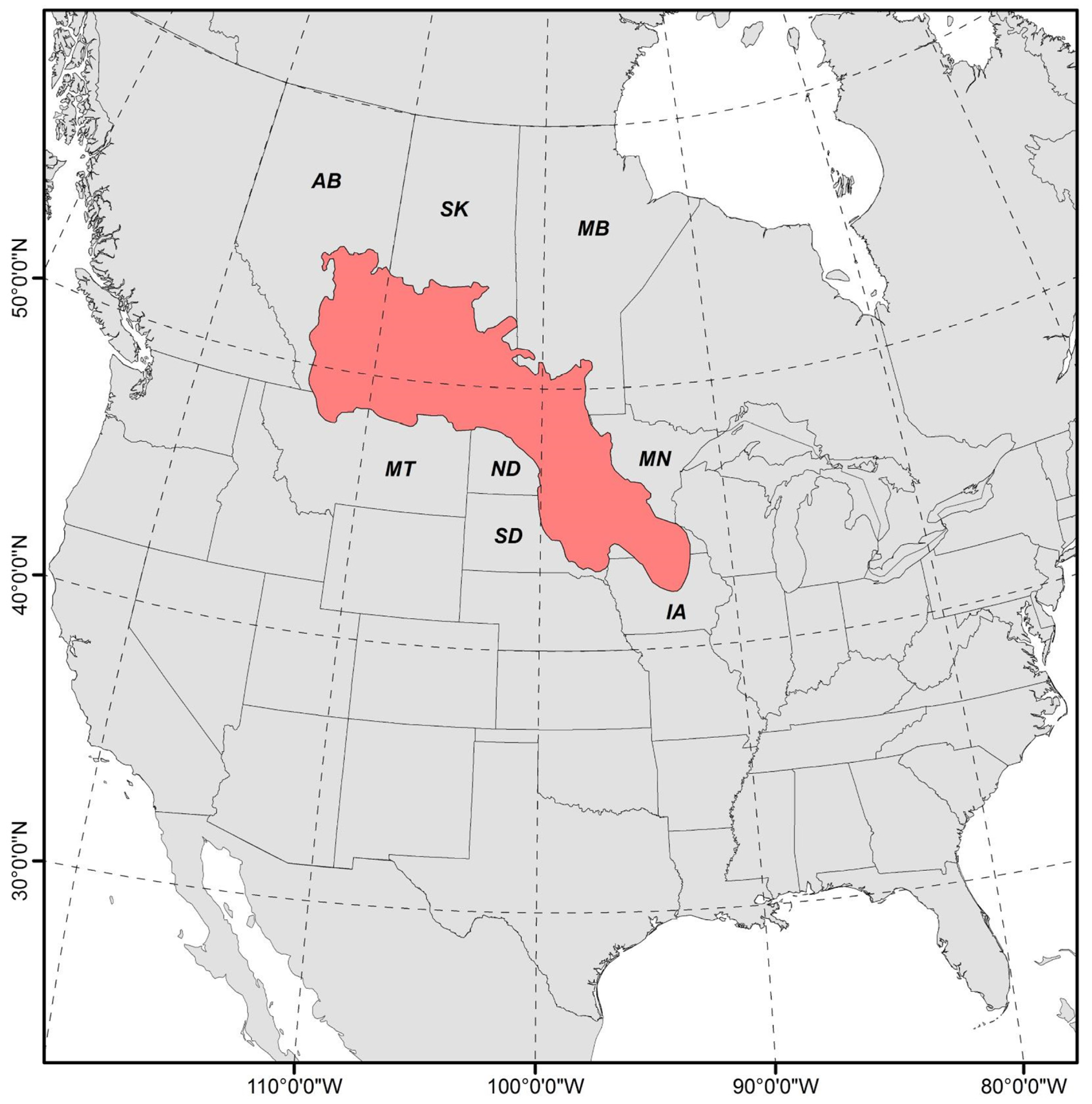
Closed-basin water bodies in the semi-arid parts of southern Canada and the Northern Great Plains of the United States occur as wetlands, ponds and larger lakes. The numbers of these waterbodies is in the millions with water areas ranging from tens of square meters to hundreds of hectares [20]. These waterbodies are especially well developed in a region of central North America called the Prairie Pothole Region (Figure A1 in Appendix).

The water balance of waterbodies in prairie pothole setting is dominated by snowmelt and summer precipitation (major inflow) and evaporation (major outflow) [17]. Thus, water levels of these potholes are commonly variable [17,18], affected by short-term, annual and inter-annual variations in precipitation and evaporation and longer-term cycles in climate [21].

2.1. Conceptual Groundwater/Lake Model

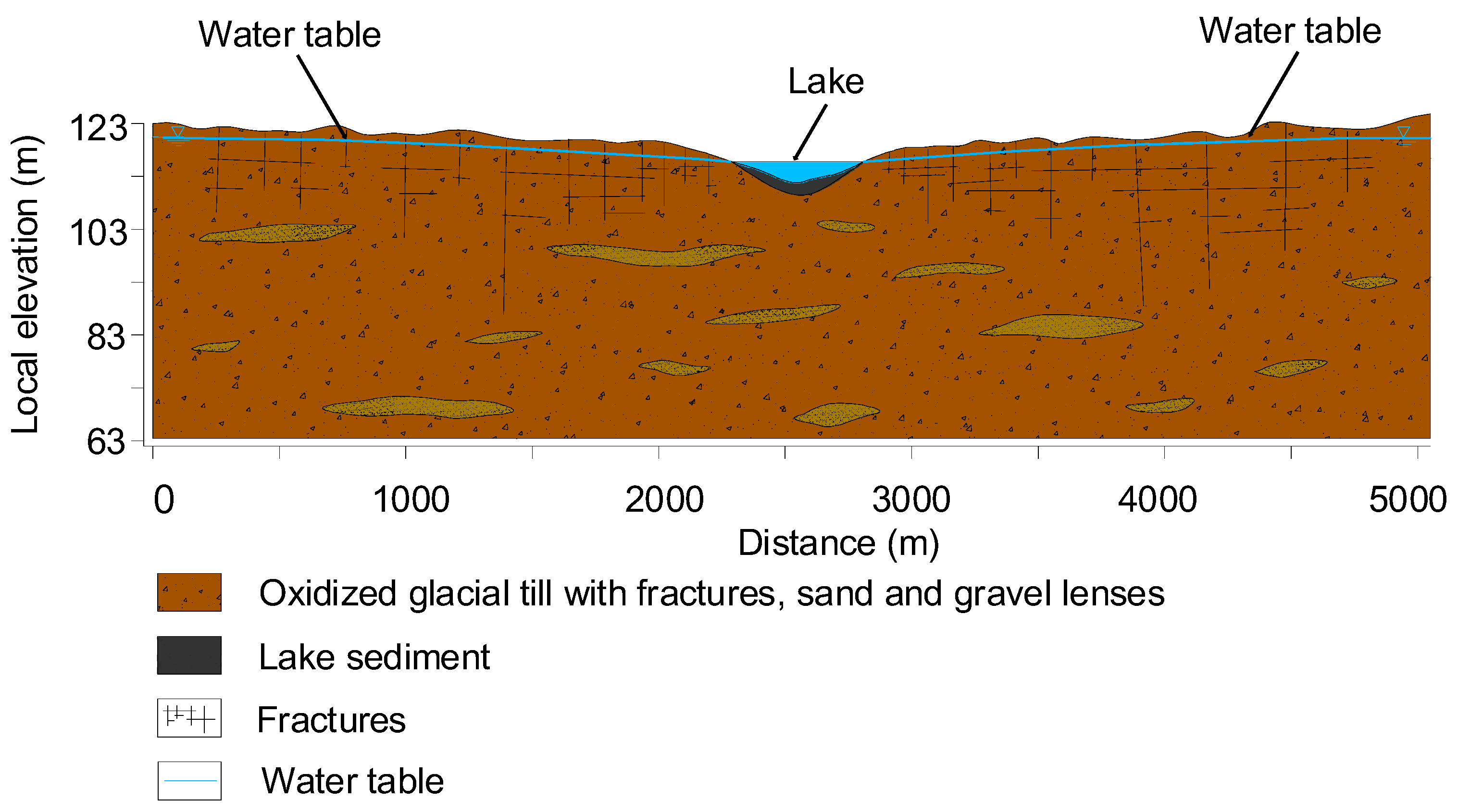
The conceptual model for our theoretical study here is based on an idealized representation of closed-basin, lake setting typical of those found in the Prairie Pothole Region just described (Figure 1). The lake-watershed is assumed to be circular in shape with a fixed radius of 5 km. The base case for the hydrogeologic setting provides a simple case of geological layering with a single till unit 60 m thick. The closed-basin lakes commonly observed in the Prairie Pothole Region associated with glacial till (Sloan, 1972) [22]. The permeability of the till is assumed to be enhanced by sand and gravel lenses, and fractures. The vertical hydraulic conductivity of the lakebed is considered as an adjustable variable in the simulation trials.

To reduce the complexity in the interpretation of the simulation results, the only inflow components to the lake considered are precipitation falling on the lake and groundwater inflow. Evaporation provides the only outflow from the lake. The lake-watershed is conceptualized as a closed groundwater basin. In other words, no water moves across the side and bottom boundaries. Water is able to enter the system across the upper boundary (Figure 1) as recharge or to leave as evaporation. This set of boundaries and pattern of recharge and discharge creates a situation where all groundwater flows towards the lake.

Figure 1. The conceptual model shown in cross-section.

Figure 1. The conceptual model shown in cross-section.

2.2. Modeling Approach

The general approach for estimating response times involves perturbing a steady state lake–groundwater system by increasing recharge until a new steady state is achieved. This approach is implemented using a transient model of groundwater flow, similar to Schwartz et al. [23]. Here, the modeling is performed with the well-known U.S. 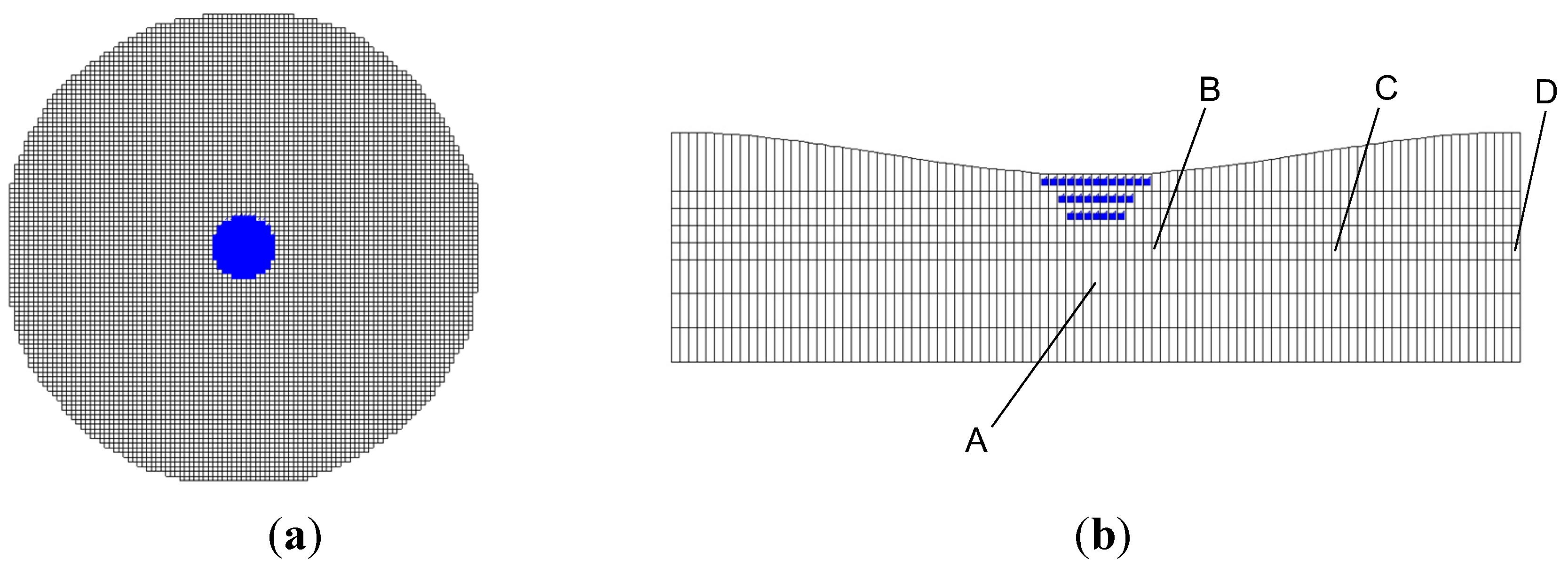Geological Survey (USGS) code MODFLOW-2005 [24], as implemented in GMS9.2 groundwater flow model [25,26,27,28,29]. MODFLOW-2005 is a 3-D, finite-difference, groundwater model for flow with capabilities for modeling surface water interactions. We couple the lake to the groundwater system using the Lake Package (LAK7), a part of MODFLOW-2005 computing the stage in the lake based on the water budget, which is a function of inflow and outflow resulting from heads differences between the lake and the aquifer. Because the lake is defined in terms of MODFLOW’s row and column grid, the shape of the lake basin is highly idealized. In our implementation here, the lake can spread but only rising through a series of steps in an idealized basin. The groundwater-lake system is discretized by square grid (50 m × 50 m) consisting of 101 columns and 101 rows and constructed using the Grid module of GMS9.2 software (Figure 2a). The system is discretized vertically in terms of 8 layers of varying thickness (Figure 2b). The top or first layer was set to capture the topographic features as well as the possible positions of varying water table. The 2nd–5th layers, where the lake cells are located and the groundwater and lake interact, have finer grids/cells vertically than the 6th–8th layers. Also shown in Figure 2b are index cells (A–D), where head values are printed for various comparisons. 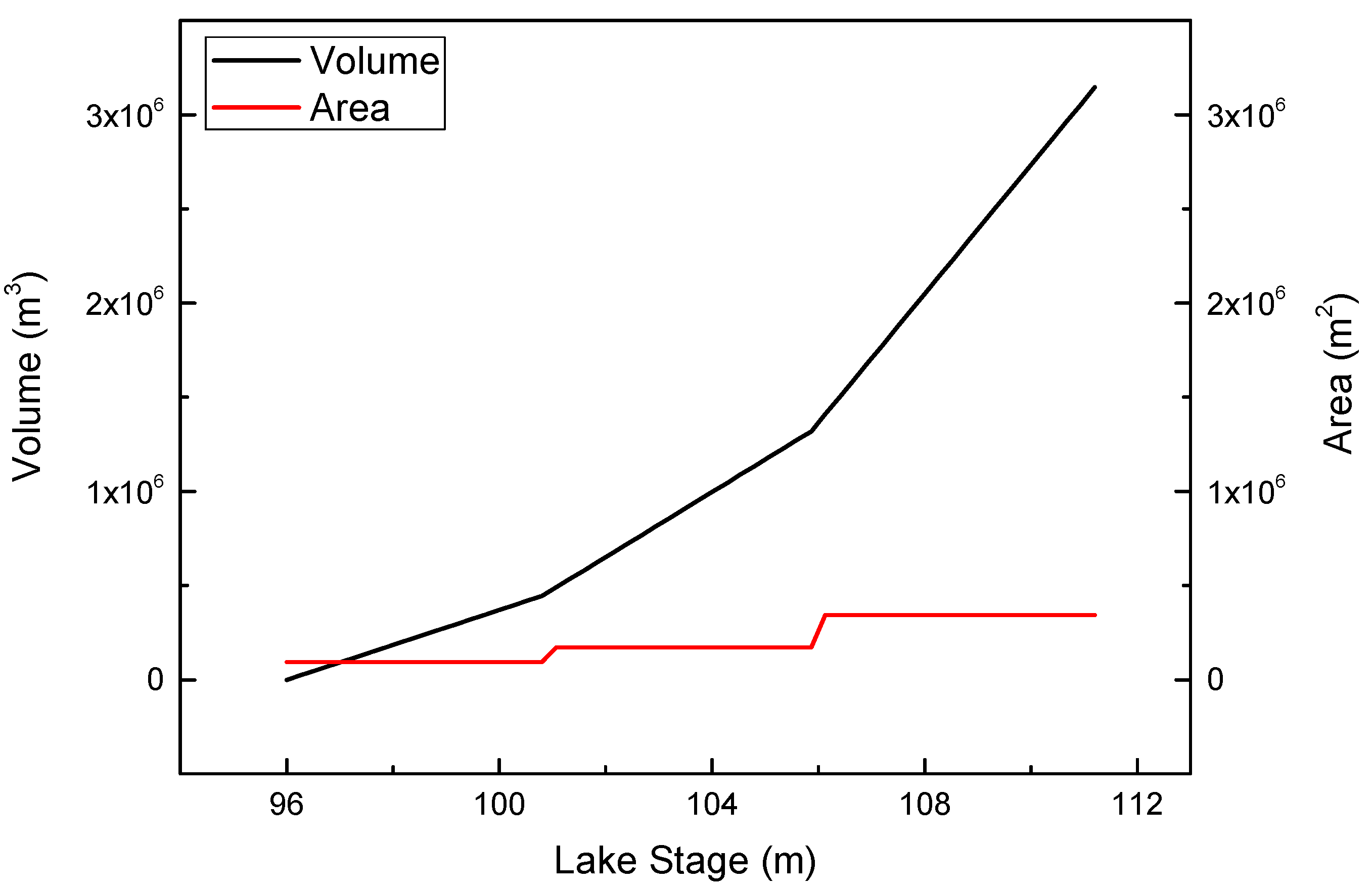Figure 3 depicts the relationships among the lake volume, area, and stage.

The hypothetical aquifer is unconfined with the water table forming the top boundary of the system. The simulations involve a uniform recharge applied to the water table. The groundwater-lake system is perturbed by an instantaneous step-increase in recharge. It is assumed that precipitation is equal to recharge, which implies no runoff.

Running MODFLOW requires model parameters such as recharge rate, evaporation rate, hydraulic conductivity, values of specific yield and specific storage, etc. In the model, the uppermost layer receives specific yield values, while deeper layers are assigned specific storage values. Evaporation from the saturated groundwater system can occur, although the rate of evaporation is assumed to decline linearly to some extinction depth.

Figure 2. Panel (a) shows a top view of the grid with a lake positioned in the center of a circular watershed. The circular basin has a diameter of 5 km. Panel (b) shows 8 model layers with lake cells indicated by blue shading. A–D indicate reference cells where hydraulic head values are used to calculate response times.

Figure 2. Panel (a) shows a top view of the grid with a lake positioned in the center of a circular watershed. The circular basin has a diameter of 5 km. Panel (b) shows 8 model layers with lake cells indicated by blue shading. A–D indicate reference cells where hydraulic head values are used to calculate response times.

Figure 3. Depth–area–volume curves for the hypothetical lake.

Figure 3. Depth–area–volume curves for the hypothetical lake.

2.3. Time Lag Calculation

As discussed in the introduction, the concept of a response time or time constant is well developed in relation to the theory of groundwater flow and lakes (e.g., Liu and Schwartz [14]). In practice, the time required for hydraulic heads in a flow system to readjust to a perturbation can be determined from a set of measurements, for example, from water-level measurements in a piezometer [1] or in a lake [12]. An alternative approach that we use here involves estimating response times from time series of simulated heads and lake levels. In either approach, the response time is defined on the basis of a characteristic associated with the mathematical function that fits the time series. Hvorslev [1], as well as others, e.g., [14,23], found that an exponential function works well. Equation (1) is of that form [23],

$$h\left(t\right)=h_0+\left(h_1-h_0\right)\left[1-e^{-t/\tau }\right]$$

(1)

where h(t) is hydraulic head h (m) at time t (d), and h₀ and h₁ are hydraulic heads at t = t₀ and t₁, respectively. The response time, denoted by τ, is the time required to accomplish approximately 63% of the total adjustment due to the applied perturbation. The flow system is assumed to have completely readjusted when t = 5τ, providing enough time for over 99% of the adjustment to be completed.

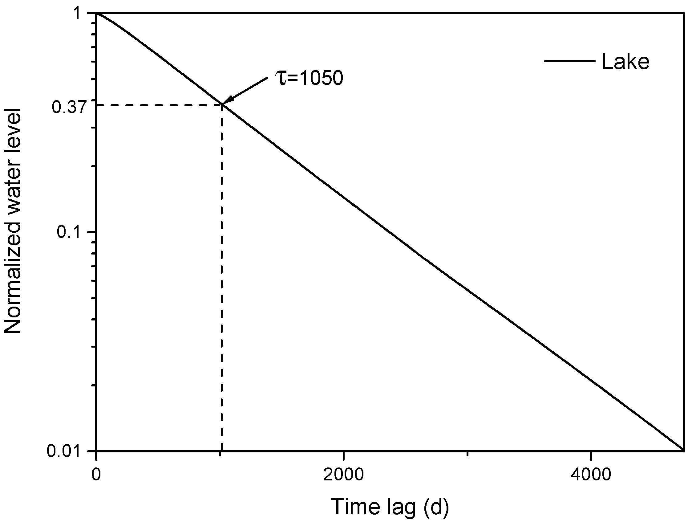
A graphical approach is used here to estimate response time for the lake or reference points in the groundwater system. A normalized time series of head ratios, which ranges between 1 and 0 is plotted as a log versus time. If the best fit is linear, then the response time is given as the time corresponding to a head ratio of 0.37 (Figure 4). With time steps of one day, this simple graphical approach provides an accurate estimate of response times.

Figure 4. Demonstration of how lake’s response time is estimated based on a normalized time series of water level.

Figure 4. Demonstration of how lake’s response time is estimated based on a normalized time series of water level.

2.4. Numerical Experiments

The numerical simulations were based on a set of model parameters described and listed in Table 1. Values of these parameters presented in Table 1 represent a setting considered to be a base or reference case. To understand the impact of some key features of hydrogeologic settings on response times, three groups of experiments were carried out, with Groups K, L, and R examining the effects of hydraulic conductivity, lakebed leakance, and recharge rate, respectively (Table 2). There are many other parameters that might also be evaluated. These, for example, might include spatial discretization [30] or heterogeneity of key units [31]. We purposely restricted our analysis to the small set of key hydraulic parameters to provide a limited scope that matches the prospective focus of this preliminary study. For example, examination of the influence of geometric parameters will require a more sophisticated modeling approach that will more realistically represent local and regional scale variability in surface topography and other features.

The basic setting represents a homogenous case with a unique value of hydraulic conductivity and lakebed conductance. The variability in hydraulic conductivity is obviously small, considering the natural range in hydraulic conductivity for natural materials. We purposely kept the variation small to prevent the system from becoming substantially different, inserting other effects that would add complexity to the interpretation. Because lake sediments are usually less permeable than the underlying aquifer, we examine the lakebed conductance of 10 and 50 times smaller than that of the base case. In this study, the recharge rate is less than lake evaporation simply because, in much of the Prairie Pothole Region, evaporation or evapotranspiration exceeds precipitation, averaging negative effective moisture of −0.33 m/year during a 20-year period of 1981–2000 [20].

Table 1. Values of hydrological and hydraulic parameters for base case.

Base Case			Stress Period 1 (0–5000 days)	Stress Period 2 (5000–20,000 days)
Aquifer	Hydraulic conductivity (m/day, or m/day)		0.6	0.6
	Recharge (mm/year)		30	200
	Evapotranspiration	Max rate (mm/year)	800	800
		Max depth (m)	1.5	1.5
Lake	Initial stage (m)		107.9	107.9
	Lakebed leakance (1/day)		0.6	0.6
	Lakebed thickness (m)		1	1
	Precipitation (mm/year)		30	200
	Evaporation (mm/year)		800	800

Table 1. Values of hydrological and hydraulic parameters for base case.

Base Case			Stress Period 1 (0–5000 days)	Stress Period 2 (5000–20,000 days)
Aquifer	Hydraulic conductivity (m/day, or m/day)		0.6	0.6
	Recharge (mm/year)		30	200
	Evapotranspiration	Max rate (mm/year)	800	800
		Max depth (m)	1.5	1.5
Lake	Initial stage (m)		107.9	107.9
	Lakebed leakance (1/day)		0.6	0.6
	Lakebed thickness (m)		1	1
	Precipitation (mm/year)		30	200
	Evaporation (mm/year)		800	800

Table 2. Summary of the parameter settings for the numerical experiments.

Cases		Hydraulic Con-Ductivity (m/day)	Lakebed Leakance (1/day)	Recharge Rate (mm/year)
Base		0.6	0.6	30 to 200
Group K	K1	0.5	0.5	30 to 200
	K2	0.6	0.6	30 to 200
	K3	0.7	0.7	30 to 200
	K4	0.8	0.8	30 to 200
	K5	1.0	1.0	30 to 200
Group L	L1	0.6	0.6	30 to 200
	L2	0.6	0.6/10.0 or 0.06	30 to 200
	L3	0.6	0.6/50.0 or 0.012	30 to 200
Group R	R1	0.6	0.6	30 to 200
	R2	0.6	0.6	30 to 300
	R3	0.6	0.6	30 to 400

Table 2. Summary of the parameter settings for the numerical experiments.

Cases		Hydraulic Con-Ductivity (m/day)	Lakebed Leakance (1/day)	Recharge Rate (mm/year)
Base		0.6	0.6	30 to 200
Group K	K1	0.5	0.5	30 to 200
	K2	0.6	0.6	30 to 200
	K3	0.7	0.7	30 to 200
	K4	0.8	0.8	30 to 200
	K5	1.0	1.0	30 to 200
Group L	L1	0.6	0.6	30 to 200
	L2	0.6	0.6/10.0 or 0.06	30 to 200
	L3	0.6	0.6/50.0 or 0.012	30 to 200
Group R	R1	0.6	0.6	30 to 200
	R2	0.6	0.6	30 to 300
	R3	0.6	0.6	30 to 400

3. Results

3.1. Response of the Lake–Groundwater Systems to Climatic Perturbation

The results from the base case (Table 1) were analyzed to explore the time lag of groundwater system in response to change in climate (i.e., increased recharge), which is assumed to occur instantaneously at day 5000. Specifically, during the time period of 0–5000 days the system was recharged at a rate of 30 mm/year, which jumped to 200 mm/year at day 5000 onwards. In the base case, the lake stage was able to fluctuate.

Figure 5 displays the steady-state head distributions for the lake–groundwater system with assumed constant recharge rates of 30 mm/year (Figure 5a) and 200 mm/year (Figure 5b). It shows groundwater flowing from the uplands, i.e., the recharge areas away from the, towards the closed-basin lake, where discharge is occurring due to evaporation. At the original steady state (Figure 5a), the highest value of hydraulic head in the recharge areas is 116.67 m; and the lowest is found at the lake, with a head value or lake level of 107.99 m.

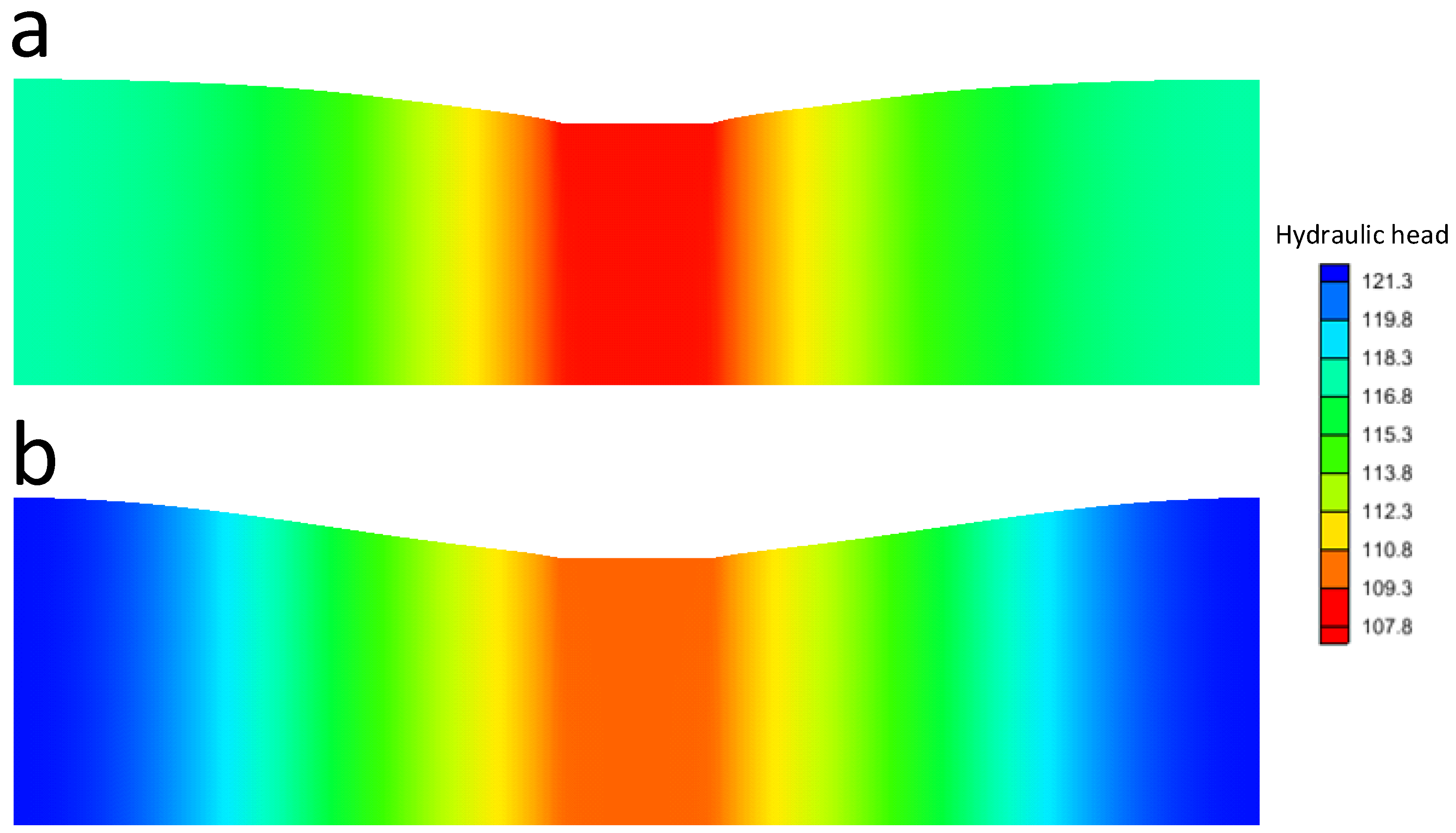
Figure 5. Cross-section representations of the steady-state hydraulic-head field and lake-water level or stage under (a) pre-perturbed and (b) post-perturbed climatic conditions.

Figure 5. Cross-section representations of the steady-state hydraulic-head field and lake-water level or stage under (a) pre-perturbed and (b) post-perturbed climatic conditions.

When the recharge rate is increased to 200 mm/year (Figure 5b), the hydraulic head values increase to a new steady-state, providing a maximum hydraulic head value at the model boundary of 121.12 m and a minimum value at the lake of 109.08 m. As expected, the hydraulic gradient towards the lake increases due to the step-increase in recharge.

The magnitude of changes in hydraulic head varies spatially in the groundwater system (Figure 5). The differences due to the adjustment in climate are larger in the recharge areas than in the discharge area. These results are evident in Figure 6, where transient changes in hydraulic heads are plotted for three reference points, D, C and B along the groundwater flow path. The step increase in the recharge rate produced the largest increase in the recharge area (D) than in the discharge area (B), close to the lake. At D, the hydraulic head values before and after the climatic disturbance were 116.67 m and 121.11 m, respectively; while at B, the head values before and after the disturbance were found to be 108.59 m and 109.53 m, respectively.

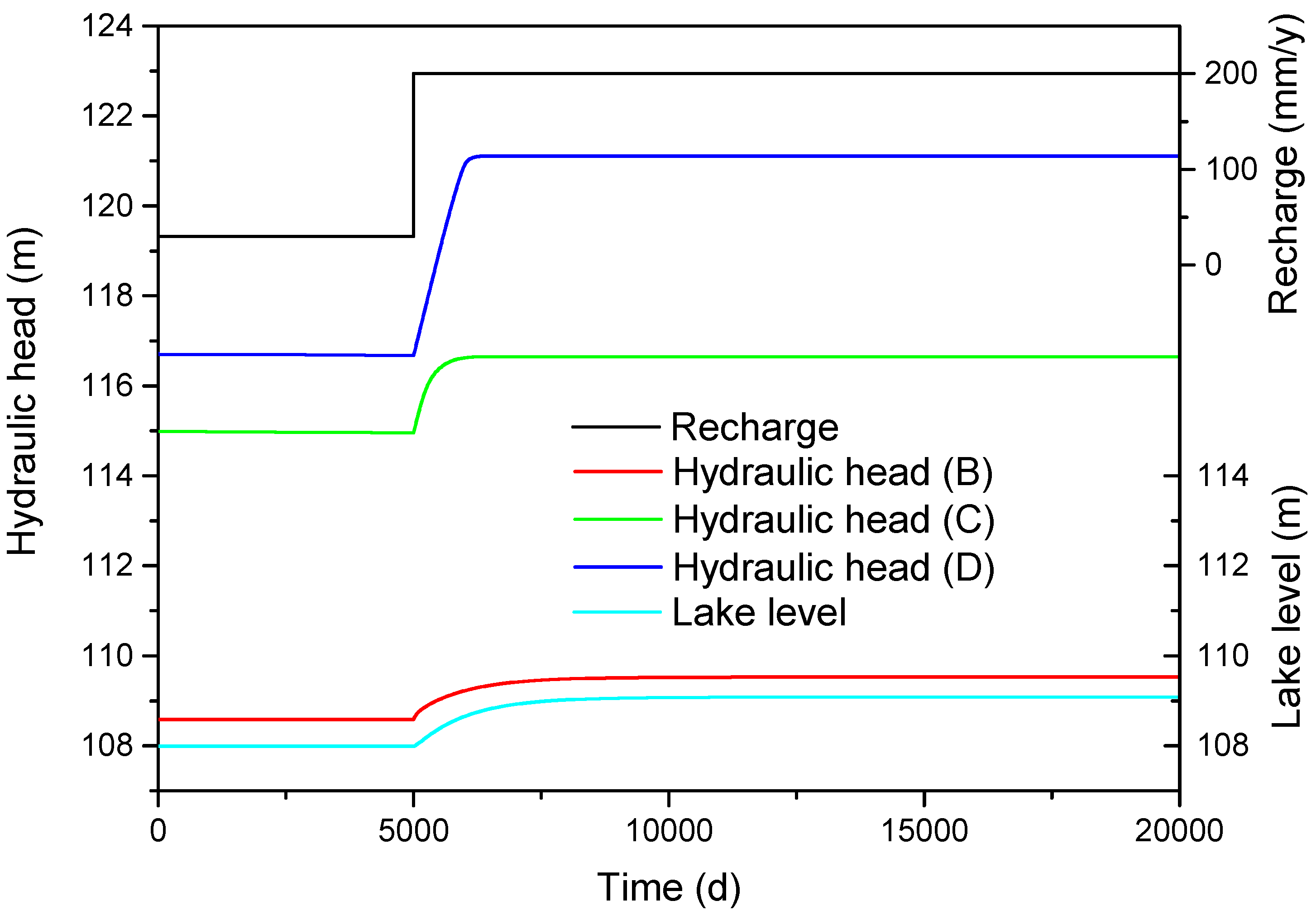
Figure 6. Time series of climatic variable (represented by recharge rate), lake stage and hydraulic head. The locations B (at lake), C (midway to basin boundary), and D (at basin boundary) are depicted in Figure 2.

Figure 6. Time series of climatic variable (represented by recharge rate), lake stage and hydraulic head. The locations B (at lake), C (midway to basin boundary), and D (at basin boundary) are depicted in Figure 2.

The lag in the adjustment of the groundwater system to the variation in climate at 5000 days was calculated for the lake and the reference points. The response time at D, C, B, A were found to be 614, 277, and 860 days and 1054, respectively. It is clear that C, located in the midway of the basin, has the shortest response time, probably due to the less head readjustment (compared to the recharge area) and the shorter distance to the recharge area (compared to the discharge area).

Similarly, the time-lag character of lake stage in response was examined by plotting the time series in lake-water level (Figure 6). The time lag in lake’s response is obviously longer than values obtained for the groundwater. More specifically, the response time of the lake was estimated to be 1050 days, which is 1.7 and 1.2 times longer than the response times found in recharge area (D) and discharge area (B), respectively.

These groundwater and lake response-time results indicate complex responses of groundwater system to the climate variability. As the recharge rate stepped up at 5000 days, hydraulic heads or water table in the recharge area away from the lake exhibited larger and faster readjustments as compared to smaller magnitude and slower responses close to the discharge area (i.e., B and A). The fastest adjustment was noted at the C profile, approximately midway between the lake and side boundary. The response time for hydraulic head adjustment under the lake (i.e., A) was 1054 days, which was nearly the same as the 1050-day response time for the lake.

3.2. Influence of Hydraulic Conductivity and Lakebed Leakance on Response Times

A variety of previous studies have identified hydraulic conductivity as being a parameter of interest for its effects on response times. Thus, this section describes results from a batch of numeric experiments (Group K, Table 2) designed to explore relationships between hydraulic conductivity and response times. Overall, runs looked at the hydraulic conductivity of the single layer and the lakebed.

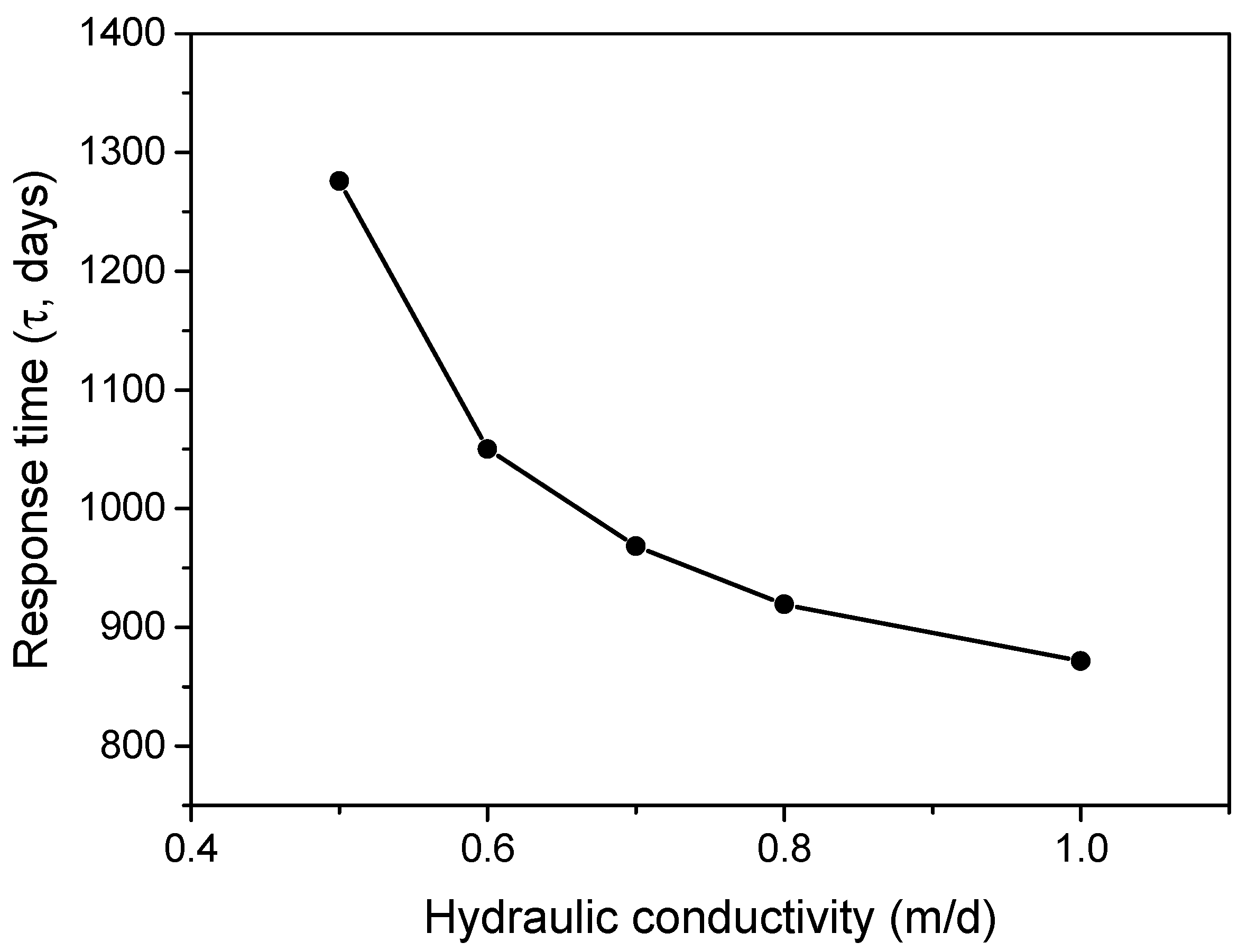
The two groups of simulation trials (Groups K and L) provided a basis for examining how changes in the hydraulic conductivity of the single layer and the lakebed influence response times. As shown in Figure 7, the response time for the lake stage is inversely proportional to hydraulic conductivity of the single layer. In other words, as the hydraulic conductivity increases, the response time of the lake decreases. For example, increasing the hydraulic conductivity from 0.5 to 1.0 m/day provided a reduction in stage response times of approximately 1276 and 872 days, respectively. The shape of the curve in Figure 7 suggests that the rate of decline is tending toward an asymptote.

Similar reductions in response times for hydraulic head were also noted. This result is not particularly surprising in keeping with results from Hvorslev [1] and the dimensional analyses of Domenico and Schwartz [3].

Figure 7. Relationship between hydaulic conductivity and the response time of lake stage to the climatic perturbation.

Figure 7. Relationship between hydaulic conductivity and the response time of lake stage to the climatic perturbation.

Another parameter affecting the behavior of the lake–groundwater system is lakebed leakance. This parameter describes how well water is conducted from the groundwater into the lake through the sediments in the bottom of the lake. Mathematically, it is the vertical hydraulic conductivity of the lakebed divided by its thickness. Given this kind of closed basin without surface runoff, the water budget is dominated by groundwater discharge and flux exchanges between the lake and atmosphere (precipitation and evaporation). Thus, intuitively, one could expect the character of surface-water and groundwater interaction to be critical to the response time of the lake.

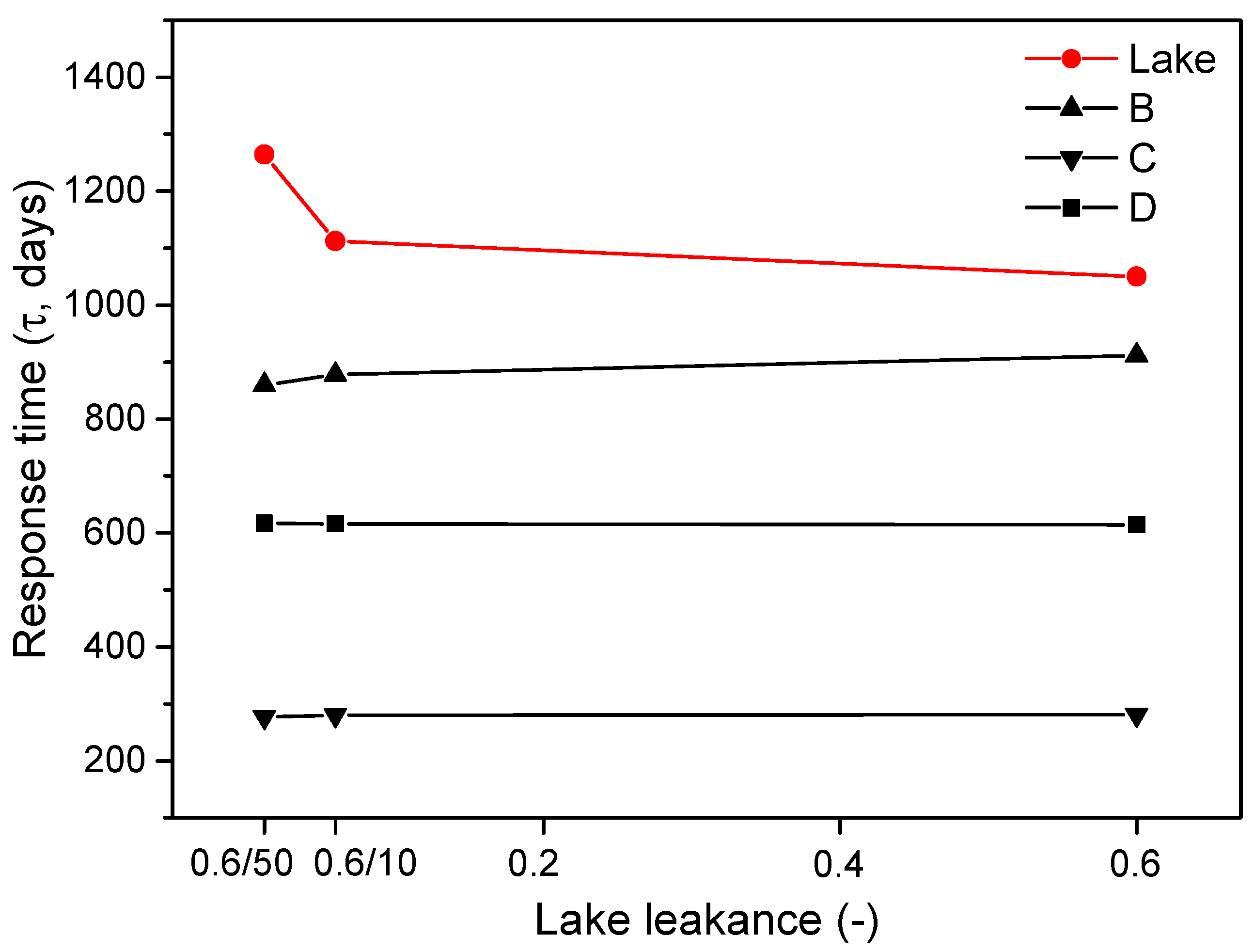
Table 2 (Group L) describes the setup of the base case and two associated model trials. The only parameter adjusted in the two model runs is leakance, which is decreased 10 times and 50 times relative to the base case. The response-time results are presented in Figure 8. As the lakebed leakance decreases from 0.6, the base case, to 10 times and 50 times smaller, the response time of the lake increases from 1050 to 1112 and 1264 days, respectively. This result indicates that reducing the connectivity between the lake and groundwater slows lake response to the step change in recharge rate.

Figure 8. Relationship between lakebed leakance and the response time of lake stage, B, C and D to the climatic perturbation.

Figure 8. Relationship between lakebed leakance and the response time of lake stage, B, C and D to the climatic perturbation.

Also shown on the figure is the response time for hydraulic head in the groundwater system, as simulated at three reference sites (B, C and D). Notice that for those sites away from the lake (i.e., C and D), the response times are different from each other but are not influenced by leakance. Moreover, the response times for the groundwater reference locations are all smaller than the lake. This result is expected because in the context of the larger groundwater system adjusting the hydraulic conductivity locally (i.e., lakebed) has a very small influence. However, the response time for B is not constant, but decreases slightly as the leakance decreases (Figure 8). This result emphasizes that changes in the coupling of the lake to the groundwater system can adjust the groundwater response times in the neighborhood of the lake. The response-time behavior for B is not particularly intuitive, given that it decreases with decreasing leakance, although the response time for the lake stage increases with decreasing leakance (Figure 8).

The simulation results for the Group L trials suggest inherent differences in the speeds of adjustment of the lake and groundwater systems to a climate perturbation. For this closed-basin problem, the groundwater system has a response time governed by features of the groundwater system, i.e., hydraulic conductivity, specific storage, which are reasonably well known. Any influences of the lake on groundwater are small and localized because it is an inherently localized feature. In contrast, the response time of the lake obviously depends on increased inflows from groundwater resulting from a wetter climate but its relatively slow response to climate change is being driven features of the lake basin (i.e., basin geometry, leakance, etc.). The Group L trials thus represent a situation where the adjustment in leakance mainly impacts the lake but not the groundwater broadly defined.

The obvious question then is why the relatively faster response time at location B is associated with a smaller leakance value. As will become clearer in the next section, hydraulic head adjustments close to the lake (e.g., B) are relatively slow because of the slow response of the lake. It appears that reductions in leakance tend to isolate the lake, pushing the hydraulic heads at B to respond slightly quicker, more in keeping with C and D. However, the fact that these adjustments are relatively small suggests that the relatively large response time at B as compared to C and D is because of slowly-responding lake nearby.

3.3. Influence of Recharge Rate on Response Times

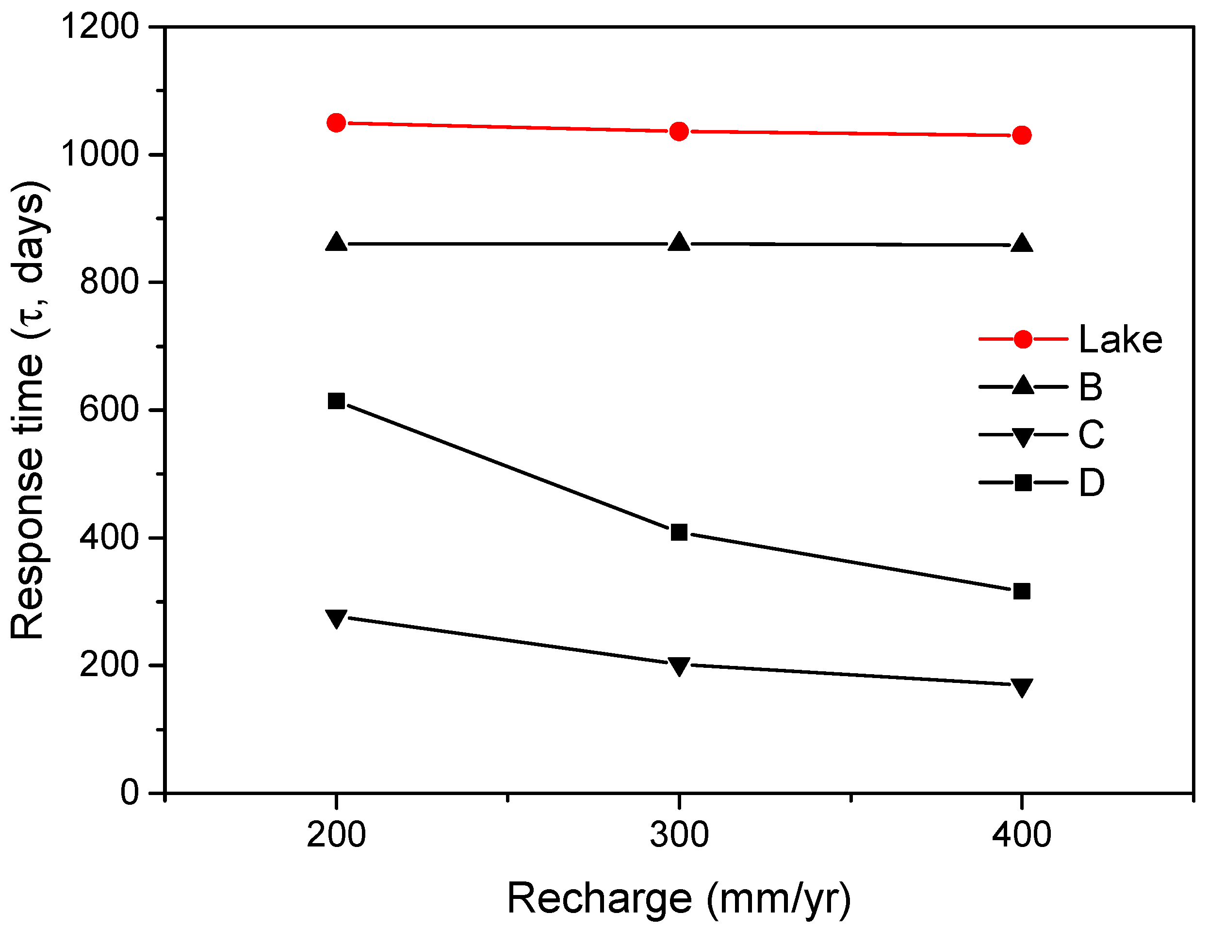
The final group of model trials Group R (Table 2) let us examine how increasing recharge rates relative to the base case influence response times for both the groundwater and surface water. The results in Figure 9 show how increasing recharge rates from the base case of 200 mm/year to 300 and 400 mm/year influenced response times. Generally, the groundwater response times at locations distal to the lake (i.e., C and D) were most influenced, showing substantial reductions as recharge rates increased (Figure 9). There was no significant change in the response times of the lake and reference grounwater locations proximal to the lake (B shown in Figure 9, A not shown).

Figure 9. Relationship between recharge and the response time of lake stage, B, C and D to the climatic perturbation.

Figure 9. Relationship between recharge and the response time of lake stage, B, C and D to the climatic perturbation.

This behavior is opposite to what was observed with lakebed leakance, where the lake-stage response times changed substantially, but not the groundwater, except close to the lake. The coupled system thus exhibits complicated behaviors with parameters driving the lake system and the groundwater system, somewhat independent of one another.

4. Discussion

High-resolution reconstructions of climates using lake sediments have contributed significantly to the understanding millennial climate fluctuations around the world. Such climate reconstructions implicitly require that the lake fluctuations can be reliably linked to climate variability. This behavior occurs in semi-arid areas where climate drives changes in the salinity, linked primarily to the balances between fresh water inflows and evaporation. However, it is likely that complexity will affect the behavior of a lake in obvious and not so obvious ways. The cumulative effects in some circumstances will weaken the connection between, for example, fluctuations in salinity and fluctuations in climate. In this respect, response time has emerged as a significant system descriptor.

As used in this study, response time describes the time required for characteristic hydraulic parameters of lake–groundwater systems (e.g., stage, hydraulic head) to readjust to a hypothetical change in climate. The concept of response time not only applies to hydraulic parameters but also geochemical parameters that influence characteristics like lake salinity. Knowledge of response-times is particularly relevant to lake behaviors. If the time lag is long (e.g., many decades to centuries), the present status of a lake and the resulting climate signal being preserved in the sediment may be some climate of the past.

In effect, as time lag increases, the ability of a lake to function as a climate recorder becomes more and more impaired. This is the same problem noted by Hvorslev [1], where poorly designed piezometers with large basic time lags produced erroneous groundwater hydrographs. Excessive time lags not only lead to a loss of signal sensitivity (i.e., smaller hydraulic head fluctuations) but also a phase shift forward in time. In other words, a peak observed today in some parameter actually will have occurred at some time in the past and have been larger than present indications [11]. As should become clear shortly, there are analogies between the efficacy of piezometers serving as measuring devices for hydraulic head and lakes to serve as climate recorders.

Our study shows how simulation results, expressed as hydraulic head for the groundwater system and lake stage, could be interpreted in terms of hydraulic response time. It represents a next step to discover the origin of time lags that have been interpreted from observations of prairie lakes [11]. The results showed that the readjustment of the groundwater flow system lagged relative to the stepped increase in climate. However, as other studies have found, the response time is not uniform within the system. The distal parts of the groundwater system responded more slowly than areas midway between the lake and basin boundary. It appears that the response time depends in part on the magnitude of head readjustment required. The groundwater system close to the lake has a response time that is longer than zones more distal. Evidently, the longer response time associated with lake stage influence nearby groundwaters.

In several respects, the behavior of the combined lake–groundwater system exhibits behaviors similar to Hvorslev’s concept of basic time lag applied to piezometers. First, Hvorslev found that usually a groundwater system tends to readjust relatively more quickly than the piezometers, especially when features of the piezometer construction are non-optimum and dominate the piezometer response. In our simulations, the time required for readjustment of the groundwater system was shorter than lake system. The longer response time for the lake is created because like the piezometer some significant volume of water needs to be transferred from the groundwater to produce the required stage adjustment in the lake and that takes time. For example, reducing the leakance of the lakebed directly slows down the pace of stage readjustment by reducing inflows to the lake. The relatively crude, cell-based, lake model probably underestimates this effect, because lateral flow can still take place into the lake without a bed. Thus, future studies will need to portray the lake in a more geometrically realistic manner.

The response of the coupled lake and groundwater system as a function of differing recharge rates is complicated. For this system, the response time required for the adjustment of the groundwater system was a function of both the adjustment time for the lake and the time required for the propagation of hydraulic head caused by the rise in the water table in the recharge area. The slower response times of the lake as compared to changes due to water-table rise was felt adjacent to the lake, causing the groundwater readjustments to be slower. Away from the lake, faster times for readjustments were calculated because the slower response time of the lake was less important. Even more complicated behaviors might be expected for situations where evaporation from both the lake and shallow groundwater might be needed to accommodate even higher recharge.

It is likely the bathymetry of the lake basin will also play an important role. For example, with a steep-sided lake the lake may need to rise considerably to expand the surface area to provide the increased evaporation matching the larger recharge. If the lake is unable to expand appropriately, then it may need to create a stage that facilitates the evaporation of shallow groundwater.

It is clear that the study here has been limited to some extent by the simplicity of the conceptual model. For example, the assumption of negligible surface runoff represents an idealized case with low-intensity rainfall. Similarly, the assumptions of a rather simple geologic setting, and a single, closed-basin lake provided additional simplicity as well. These choices and others, however, were made intentionally so as not to create so complicated a system/setting that relationships between causes and effects would be difficult to sort out. In this respect, our paper here follows well known studies of simple systems provided, for example, by Tóth [32] and Winter [33]. The obvious next step will be adding back this complexity within the framework of a much more complicated modeling system.

5. Conclusions

The simplified simulation results presented and discussed here hint at the complexity of lake behaviors in response to climatic adjustments. The focus in our study was on hydraulic controls that can impact both groundwater and lake systems. Although obviously coupled, the response times of the lake and groundwater systems were different from one another because the critical parameters controlling the response-time behavior of the groundwater system (e.g., recharge rate) differed from those controlling the response-time behavior of the lake (e.g., bed leakance). Response times for groundwaters close to the lake were controlled by the lake because of the slow transient response in stage. However, the influence of the lake declined toward the basin boundaries.

The next step in future studies is to consider other sources of time lag. Potential problems for consideration are (i) hydraulic readjustments through a cascade of coupled lakes and groundwater systems or (ii) response times in mass transfers that operate to adjust lake salinity. In these and existing conceptualizations, processes are likely to be hysteretic in the sense that response times for lake stage will likely change depending upon whether the climate change leads to wetter or drier conditions.