Article

Characterizing the Impact of River Barrage Construction on Stream-Aquifer Interactions, Korea

1
Division of Earth Environmental System, Pusan National University, Busan 609-735, Korea
2
Korea-CO2 Storage Environmental Management (K-COSEM) Research Center, Department of Earth and Environmental Sciences, Korea University, Seoul 136-701, Korea
3
Groundwater Department, Korea Institute of Geoscience and Mineral Resources (KIGAM), Daejeon 305-350, Korea
4
Hydro Science and Engineering Research Institute, Korea Institute of Civil Engineering and Building Technology (KICT), Goyang 411-712, Korea
*
Author to whom correspondence should be addressed.
Water 2016, 8(4), 137; https://doi.org/10.3390/w8040137
Submission received: 4 November 2015 / Revised: 31 March 2016 / Accepted: 1 April 2016 / Published: 7 April 2016
(This article belongs to the Special Issue New Developments in Methods for Hydrological Process Understanding)

Abstract

:
This study investigated changes in stream–aquifer interactions during the period shortly after the construction of the Changnyeong-Haman River barrage (CHRB) on the Nakdong River in South Korea. The hydraulic diffusivity (α) and river resistance (R) values at the semipervious stream–aquifer interface were estimated by using a one-dimensional (1-D) analytical solution with Fourier transform (FT). Prior to the application of the 1-D analytical solution, the noise effects on the groundwater levels were removed by using fast Fourier transform and low-pass filtering techniques. Sinusoidal variation of the river stages was applied to the 1-D analytical solution. For the study period, the R values showed a decreasing trend, while the α values showed an increasing trend, and results showed that the average of the median values of flood duration times (td) and flood amplitudes were reduced to 78% and 59%, respectively. Moreover, the ratio of flood peak time to td demonstrated a decreasing tendency after the construction of the CHRB. Hence, it is concluded that the dredging and increase of river-water storage due to CHRB construction enhanced stream–aquifer interactions during the period shortly after the construction of the CHRB.

1. Introduction

Stream–aquifer interactions have been studied under various settings such as during regional groundwater management projects [1,2], contaminant transport and remediation investigations at the stream–aquifer interface [3,4,5], projects aimed at estimating hydraulic parameters [6,7,8,9,10], and investigations of the hydraulic connectivity between a stream and an aquifer system [11,12,13,14]. In particular, stream–aquifer interactions have increasingly become a critical issue for water resources management and such interactions are now being emphasized in applications involving hydrological, environmental, ecological, and hydrogeological problems in the riparian/hyporheic zone. In the riparian/hyporheic zone, the recharge process of an aquifer takes place because of inflow from the stream and this process is influenced by stream level fluctuations [15,16] and rainfall infiltration/percolation into saturated beds [17]. Direct inflow from a stream should contribute predominantly to groundwater level rise near the stream. Additionally, artificial effects such as the construction of a dam, dredging of the riverbed, and agricultural activities can also strongly affect stream water–groundwater mixing and thus cause changes in flux, hydraulic head gradients, and boundary conditions in the riparian/hyporheic zone [18,19,20]. Hence, variation in groundwater level rise induced by natural and artificial factors should be considered when simulating stream–aquifer interactions.
Groundwater level response induced by an arbitrarily and temporally fluctuating stream stage should be evaluated with precise data in order to understand the stream–aquifer interaction process. However, in spite of complex, arbitrary, and temporal changes in a stream stage, simplified analytical solutions are typically utilized for evaluating the aquifer response induced by water level variations, which are often modeled with linear, unit-step, and sinusoidal patterns [6,21,22]. Early analytical solutions for estimating aquifer hydraulic properties were derived from analogs of the heat conduction problem [23,24]. The convolution method has been used to simulate groundwater response to randomly varying stream fluctuations [22,25]. Groundwater level fluctuations caused by flood events are produced by both the effects of pressure propagation and recharge. The groundwater level fluctuation induced by a stream floodwave is dependent on several factors in the alluvial and aquifer environments, such as the channel and aquifer geometry, base level of the groundwater table, thickness of the vadose zone, hydraulic properties of the aquifer, stream–aquifer connectivity, stream flood intensity and duration time, bank storage capacity, and hydraulic gradients [26,27]. Floodwave response techniques (FRTs) for the stream–aquifer interaction region have been widely used to estimate aquifer properties [6,7,8,9,10,11,12,21,22,25,28]. However, boundary conditions of the stream–aquifer interaction region are not easy to determine because of the uncertainty in regard to aquifer geometry, as well as the geological heterogeneity and anisotropy. Fourier transform (FT) is one useful method that can be used to convert complex boundary conditions to simpler ones of infinite extent in one direction [23,24].
The hydraulic head fluctuation through an alluvial aquifer during stream flood events generally has been handled by kinematic waves based on the law of mass conservation through the continuity equation and flux concentration [27,29,30]. Garcia-Gil et al. [27] separated background groundwater head and kinematic groundwater head due to floodwaves by applying the superposition principle. However, dynamic wave propagation accompanying solute transport, which is based on the non-conservative characteristics of delaying and damping through the aquifer [15,26,31], has often been considered. Noise effects on groundwater level fluctuations like those from rainfall percolation, tidal effects, seasonal and annual variations of groundwater levels, agricultural pumping, irrigation and drainage, and dam operations should be eliminated in order to precisely evaluate the effect of the stream floodwave on the aquifer.
Only a few studies of stream–aquifer interactions have been executed by using actual flood events, in comparison to intensive studies of stream–aquifer interactions through the use of theoretical approaches [11,16,20,30], and a limited spatial range exists for field application data collected with a limited numbers of piezometers [11,16,32,33]. Because of these limited data, there is currently an insufficient understanding of complex stream–aquifer interactions and how stream floodwaves propagate to aquifers over time [26,32]. Therefore, sufficient spatiotemporal data will be necessary to describe the changes in the response characteristics of stream–aquifer interactions accurately, especially when the hydrogeological environment of the riparian/hyporheic zone is influenced by anthropogenic impacts like dredging and dam construction.
This study aimed to characterize changes in stream–aquifer interactions shortly after the construction of the Changnyeong–Haman River barrage (CHRB) on the Nakdong River in South Korea, and the hydraulic diffusivity (α) and river resistance (R) values at the semipervious stream–aquifer interface were estimated by using a one-dimensional (1-D) analytical solution with Fourier transform (FT). This study utilized a FRT for evaluating changes in the hydrogeological environment that were not addressed in most previous studies [7,22,25,26]. Moreover, low-pass filtering (LPF) was applied to eliminate noise effects within the groundwater level data.

2. Materials and Methods
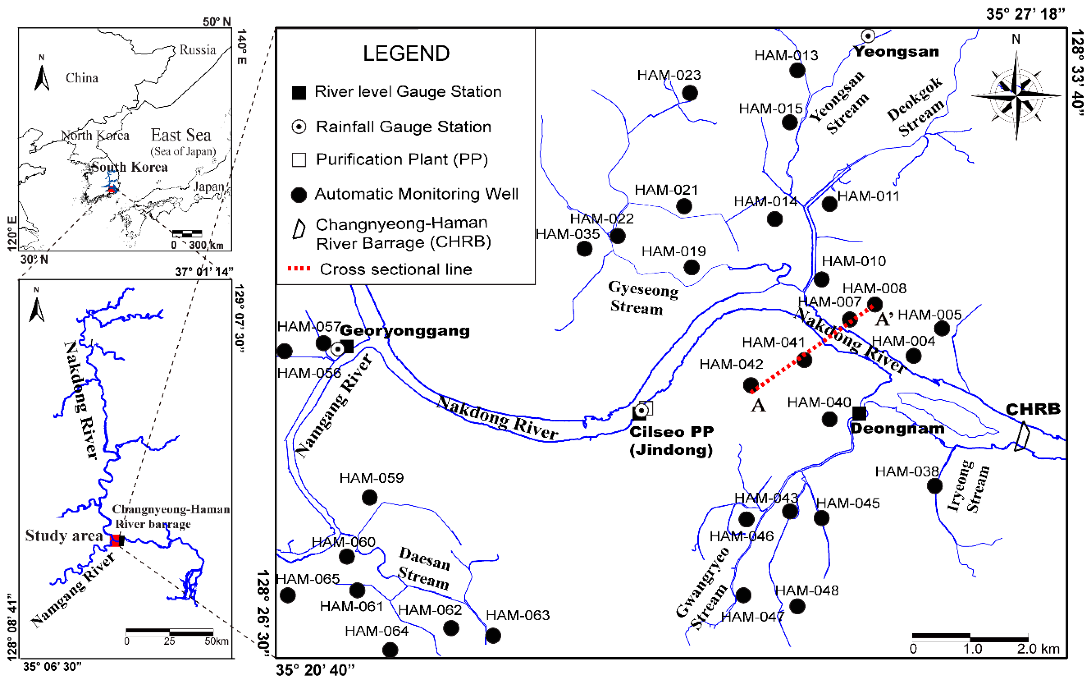
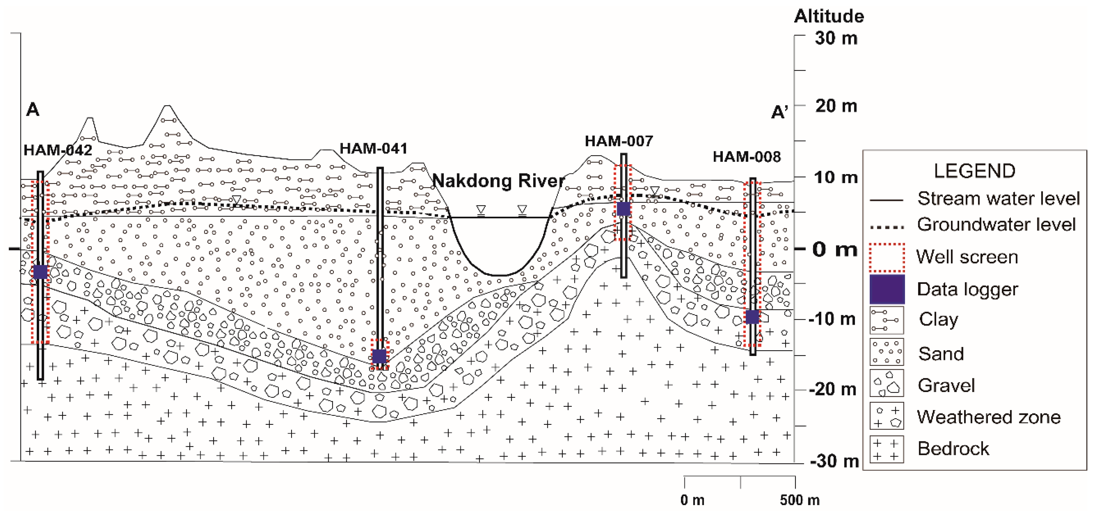
2.1. Study Area

The study area (~110 km2), which was located upstream of the CHRB, includes alluvium regions of the Namgang River, Gwangryeo Stream, and Yeongsan Stream within the Nakdong River basin (Figure 1). The Namgang River area (NG_R) is comprised of the downstream portion of the Namgang River (length of ~186.3 km) that flows from south to northeast, and the Gwangryeo Stream area (GR_S) is comprised of the Gwangryeo Stream (length of ~7.5 km), which flows from south to north, and the Iryeong Stream (length of 3 km). The Yeongsan Stream area (YS_S) is comprised of the Yeongsan Stream (length of ~9.8 km), which flows from north to south, the Deokgok Stream (length of 7.3 km), as well as agricultural areas (Figure 1). Sixteen river barrages were constructed on the four major rivers (the Han, Nakdong, Geum, and Yeongsan) in South Korea as a result of the Four Major Rivers Restoration Project (4MRRP) from 2008 until 2012 (Figure 1 and Table 1). The 4MRRP increased the width of the Nakdong River from 330 to 520 m and decreased the elevation of the river bottom from −2.0 to −5.70 m (above mean sea level, AMSL) at the CHRB site [34]. The mean discharge of the river in the dry season (November to February) at the Jindong (JD) gauge station increased from 104.7 m3/s in 2009–2011 to 178.6 m3/s in 2012–2013 as a result of the river barrage construction [35].
The Nakdong River, with a length of 525 km, flows southward from Gangwon Province to Busan City and then enters the South Sea. The river has the second largest drainage area (23,384.21 km2) of any river in South Korea. The mean discharge of the river from 2009 to 2013 was 360 m3/s, and the seasonal variability of the discharge ranged from less than 50 m3/s in the dry season (December to January) to more than 12,000 m3/s in the rainy season (June to September) [35]. The study area is composed mostly of agricultural fields with low elevations of 6–10 m AMSL, and these fields are mainly rice fields (>84%). In the study area, groundwater is commonly used for irrigation, and it is influenced by the agricultural cycle of rice cultivation from May to August as well as the cycle of greenhouse agriculture from December to April. The amount of average annual precipitation in Korea is 1357 mm (1981–2010) [36], and the amount of average annual rainfall (2010–2014) in the study area is 1249 mm; in this region, the highest monthly rainfall occurs in August (295 mm) and the lowest monthly rainfall occurs in January (8 mm), based on data from the Georyonggang, Yeongsan, and Jindong rainfall gauging stations. The rainy season (June to September) provides >64% (807 mm) of the annual rainfall, and the rest of the year provides the remaining ~36%.
Geologically, the study area is composed of the mid-Cretaceous sedimentary Hayang Group (Haman Formation and Jindong Formation), the late-Cretaceous volcanic Yucheon Group (Jusan andesite), Bulguksa igneous rocks (diorite, biotite granite, granodiorite, and granite porphyry and dikes) that intrude into the mid- and late-Cretaceous sedimentary and volcanic rocks, and Quaternary alluvium [37]. The Quaternary alluvium has an average thickness of 1 to 33 m and is distributed predominantly along the sides of the Nakdong River and its tributaries. Kim et al. [38] reported a sand layer with a thickness of 0.3 to 4 m, a gravel layer with a thickness of 1 to 10 m, and a weathered zone with a thickness of 1 to 3 m in and around the study area. On the basis of shallow hydrogeological profiles in the study area (Figure 2), the alluvial aquifer is composed of clay, sand, gravel, and weathered layers. The clayey layer showed an average thickness of 7.9 m. The thickness of the sand layer ranged from 2.0 to 20.0 m, with an average of 9.1 m, and the thickness of the gravel layer ranged from 0.0 to 14.0 m, with an average of 5.6 m. The weathered zone of sedimentary bedrock (Haman Formation and Jindong Formation) ranged in thickness from 0.5 to 15.0 m, with an average of 5.1 m.

2.2. Data Collection and Monitoring of Water Levels and Electrical Conductivity

Groundwater level (WL_G) was measured automatically at 32 monitoring wells in the riparian zones of the NG_R, GR_S, and YS_S between June 2011 and February 2013. River-water level (WL_R) was measured every hour at the Georyonggang (GY), JD, and Deongnam (DN) gauging stations (Figure 1 and Table 1). The electrical conductivity of groundwater (EC_G) and the electrical conductivity of river water (EC_R) were measured at one-hour intervals at the automatic monitoring wells and the Chilseo purification plant, respectively (Table 1). The data loggers that were used in this study consisted of the multi-sensor type (water level, electrical conductivity, and temperature), and data were automatically corrected based on the barometric pressure (MK-15CTD series) [39]. The sensors were installed at depths ranging from 6.56 m (HAM-008) to 39.7 m (HAM-004) [39]. The measured range of the water level was 0 to 70 m with a sensitivity of ±0.05%, and the measured range of EC was 0 to 100,000 µS/cm with a sensitivity of ±5% µS/cm [39].

2.3. Governing Equation for Stream-Aquifer Interactions

In a semi-infinite homogeneous isotropic confined aquifer, the groundwater level h ( x , t ) induced by the propagation of a floodwave with consideration of river resistance R [23,24] is
ϕ ( x , t ) = h ( x , t ) R h ( x , t ) x
where ϕ (x,t) is the hydraulic head (L) without river resistance, x is the lateral distance from the stream–aquifer interface (L), t is the time (T), and R is the resistance to flow conveyed by the river as a result of its semipervious bed and partial penetration of the aquifer (L), which is the distance corresponding to the piezometric head loss between the semipervious bed and river wall [21,40]. The value R is the dominant parameter for modeling the hydraulic connection between an aquifer and stream, and smaller R values are indicative of lower flow resistances across the river–aquifer interface [10,21,26]. R refers to the sum of the retardation coefficient and the resistance effect by the partially penetrated river [26,40], and it is different from the retardation coefficient proposed by Hantush [41]. Singh [21] generalized R to the following cases: (1) R = 0 (i.e., a fully penetrating river without a semipervious bed) with a symmetrical floodwave response to linear variations of WL_R corresponding to the equations of Cooper and Rorabaugh [42] and Hantush [41,43]; (2) R = 0 for long-term sinusoidal variations of WL_R equivalent to a steady periodic solution [44,45]; and (3) R > 0 (i.e., a fully penetrating river and a semipervious bed) with a unit-step rise in WL_R equal to the solution of Hall and Moench [22,40].
The governing equation of stream–aquifer interactions in a semi-infinite homogeneous isotropic confined aquifer assuming the Boussinesq approximation can be expressed as
ϕ   ( x ,   t ) t = α   2 ϕ ( x ,   t ) x 2 ,
where the initial and boundary condition at infinity, respectively, are
ϕ ( x ,   0 ) = ϕ ( , t ) = 0 ,
and the boundary condition at the river [21,23] is
ϕ ( 0 , t ) = H s ( t ) ,
Here, Hs(t) is the river stage (L) and   α is the aquifer diffusivity (L2·T−1), which is the ratio of transmissivity T (L2·T−1) to storativity S(-). The main assumptions of the 1-D analytical equation are that the aquifer parameters such as T and S are constant and that floodwaves through the aquifer are 1-D and perpendicular to flow direction [6,7,10]. The solution of Equation (2) satisfying (2a) and (2b) by the FT method is presented as shown below [23,24]:
ϕ   ( x ,   t ) =   x 2 π α 0 t H s ( τ ) exp ( x 2 / 4 α ( t τ ) ) ( t τ ) 3 / 2 d τ ,
When setting x 2 α ( t ν ) = μ , ( t τ ) =   x 2 4 α μ 2 , Equation (3) can be written as
ϕ   ( x ,   t ) =   2 π x / 2 α t H s ( t x 2 4 α μ 2 ) e μ 2 d μ ,
Equation (4) matches the analogous problem of heat conduction of Carslaw and Jaeger [23]. Continuous variation of the sinusoidal stream stage [21,24,44,45] can be generalized by a sine wave as follows:
H s ( t ) = A sin ( ω t ) ,
where A is the amplitude of the sinusoidal stream stage (L) and ω is the angular frequency (T−1). Assuming that both river and aquifer are in equilibrium prior to the river stage variation, Equation (4) is solved by a solution analogous to that of heat conduction [21,23]:
h ( x , t ) =   A [ e x p ω 2 α x sin ( ω t ω 2 α   x δ ) 2 ω 2 α     R ( ω 2 α   R + 1 ) + 1 + 1 π 0 ( ω { R ν α cos ( ν α   x ) + sin ( ν α   x ) } ( ν 2 + ω 2 ) ( 1 + ν R 2 α ) )   e ν t d ν ] ,   R 0 ,
where
δ = tan 1 ( ω 2 α   R 1 + ω 2 α   R ) ,
The second right-side part of Equation (6) becomes 0 in steady periodic conditions and after a sufficiently long time from the initiation of observations [23].

2.4. Removal of Noise from Groundwater Level Data with LPF

The fast Fourier transform (FFT) and then LPF can be applied to the groundwater level data to remove noise. The FFT is an algorithm that computes the discrete Fourier transform (DFT) of time series data, and it converts time domain data to frequency domain data and vice versa [46]. The LPF technique extracts signals with frequencies lower than a certain target cut-off frequency. For certain time series data of V, the FFT as written by Walker [46,47] is
  W n =   k = 0 N 1 V k e 2 π k n / N ,
where W is generally a complex number, n is the frequency index, N is the sample length, and k is the time series index. A general LPF has the following form [46,47]:
V f =   p = 0 P c p V k p +   q = 1 Q d q V k q ,
Here, V f is the filtered time series, and c p and d q are the filter coefficients with the summation indices of p and q, respectively. The filtered output is the weighted sum of the current and previous input number, P, and previous output number, Q [46,47]. The target frequency is selected through a frequency analysis of signal data.

3. Results and Discussion

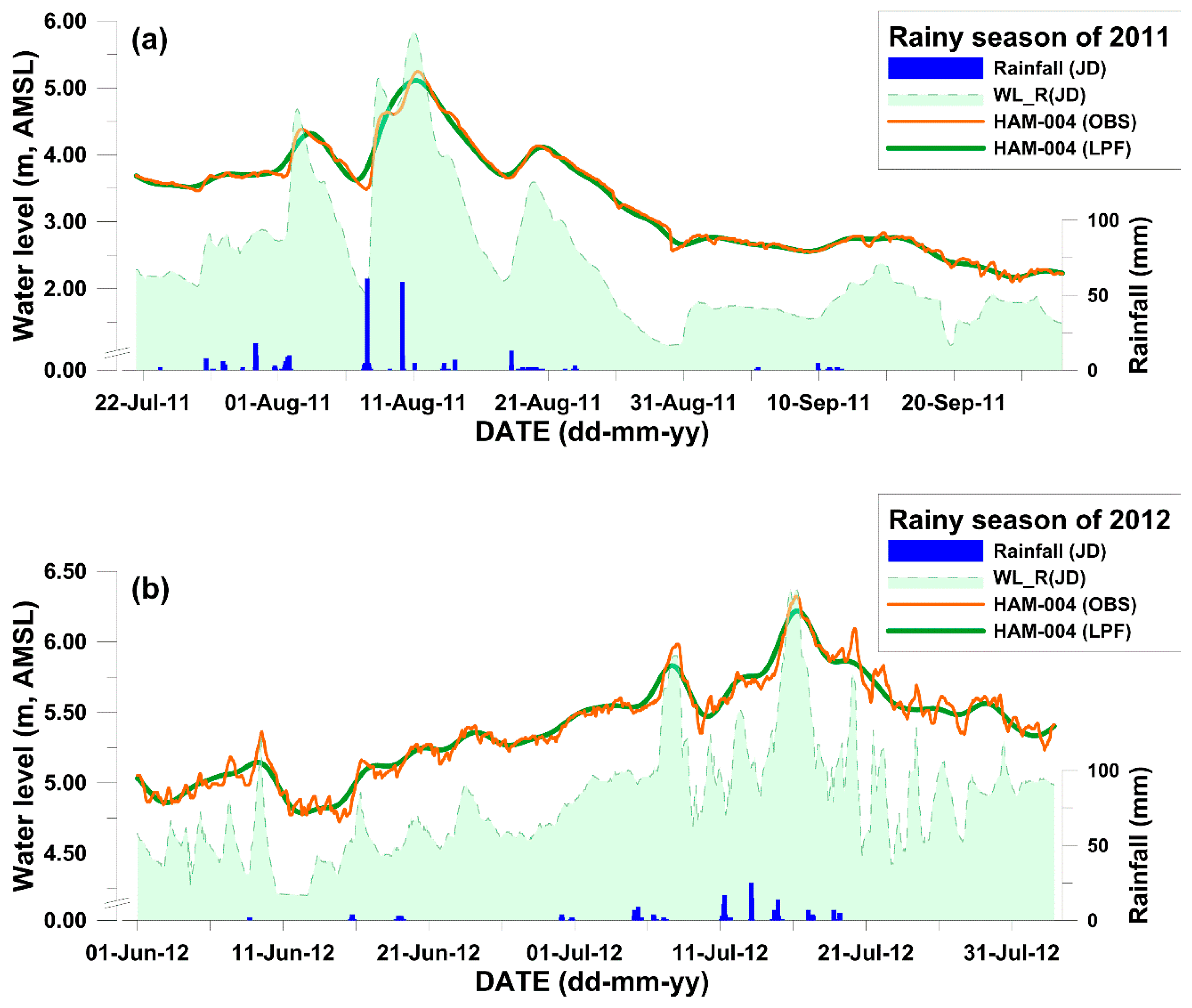
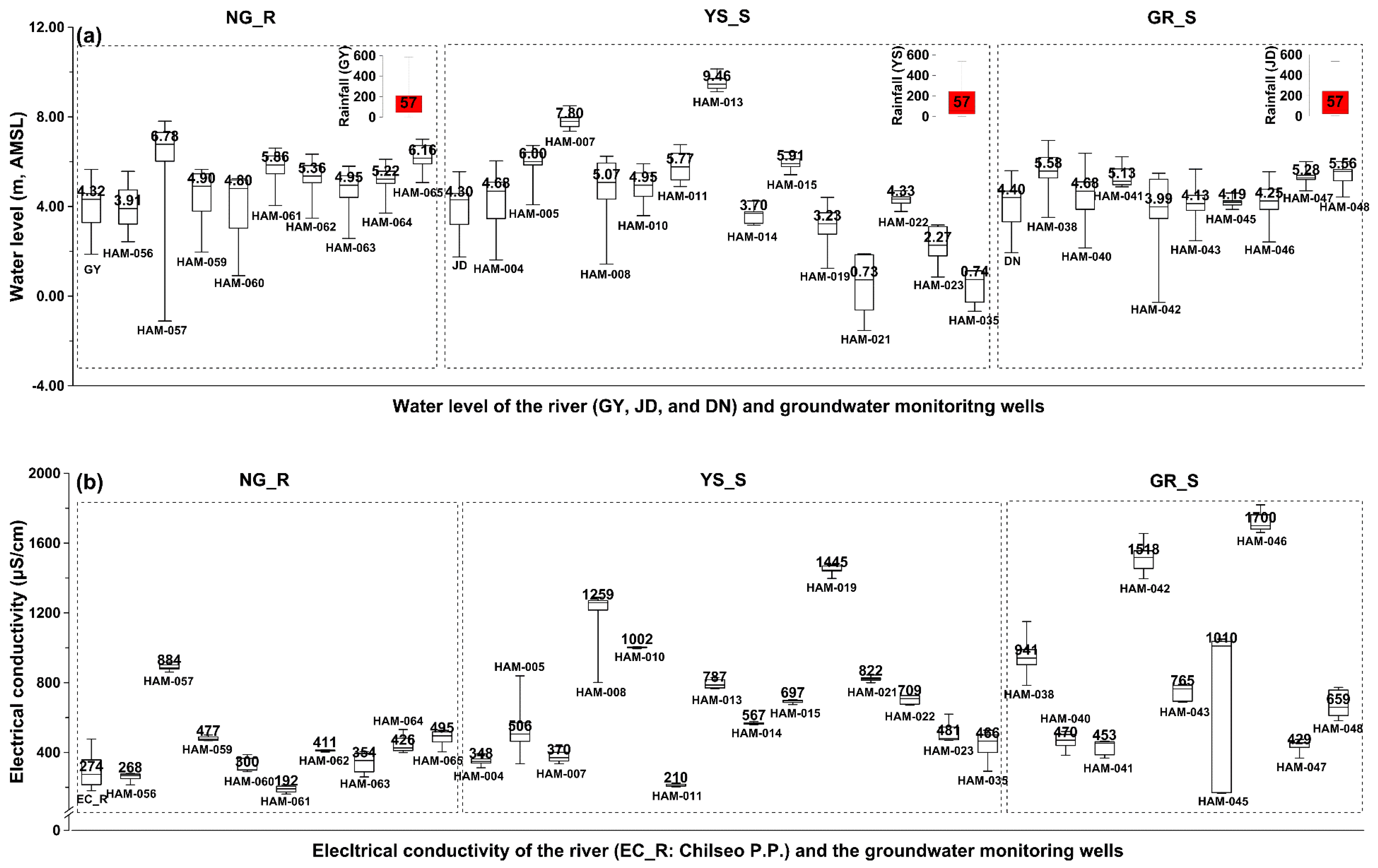
3.1. Changes in Water Levels and Electrical Conductivity

The CHRB was completed by the Korean Government on 10 December 2011, and initiation of water storage began as early as October 2011. The WL_R and WL_G increased following the construction of the CHRB. The average WL_Gs in the rainy season (June to September) of 2011 and 2012 were 4.64 m and 5.40 m (AMSL), respectively, relative to the average WL_Rs of 2.58 m and 5.15 m (AMSL) during 2011 and 2012, respectively (Table 2). Most observation well data near the Nakdong River (except for at HAM-004, HAM-019, and HAM-059) indicated that the river showed a gaining pattern except for during peak flood periods. Besides, the head difference between the WL_Gs and WL_Rs was reduced after construction of the CHRB compared to the situation before construction (Table 2). Moreover, the average difference of WL_R values between 2011 and 2012 (i.e., the values increased) was 1.87 m and the average difference of WR_R fluctuation values (i.e., the max–min values, which decreased) during the same period was 1.60 m; these values changed because of the river stage control at the CHRB (Table 2). According to the median values of rainfall, river-water levels, and groundwater levels during the observation period, relatively higher WL_Gs appeared near the river, such as at HAM-057 in NG_R, HAM-004 in YS_S, and HAM-038 in GR_S (Figure 3a). However, the WL_G data sets collected at the HAM-057 (NG_R), HAM-008 (YS_S), and HAM-042 (GR_S) wells contained noise effects due to groundwater pumping and rainfall.
The EC_G values decreased after the construction of the CHRB; the average EC_G values in the rainy season of 2011 and 2012 were 675 µS/cm and 662 µS/cm, respectively, with respect to the EC_R value (370 µS/cm) at the Chilseo purification plant (Table 2). Spatially, the median EC_G values at the locations far from the river (HAM-057 in NG_R, HAM-008 and HAM-019 in YS_S, and HAM-042 and HAM-046 in GR_S) were relatively high, thus demonstrating a strong influence of the groundwater. Conversely, the EC_G values of the locations comparatively near the river (HAM-005 in YS_S and HAM-038 and HAM-045 in GR_S) varied greatly between 175 and 1100 µS/cm, thus indicating that these were areas of groundwater–river water mixing (Figure 3b).

3.2. Evaluation of Stream–Aquifer Interactions by the Analytical Solution

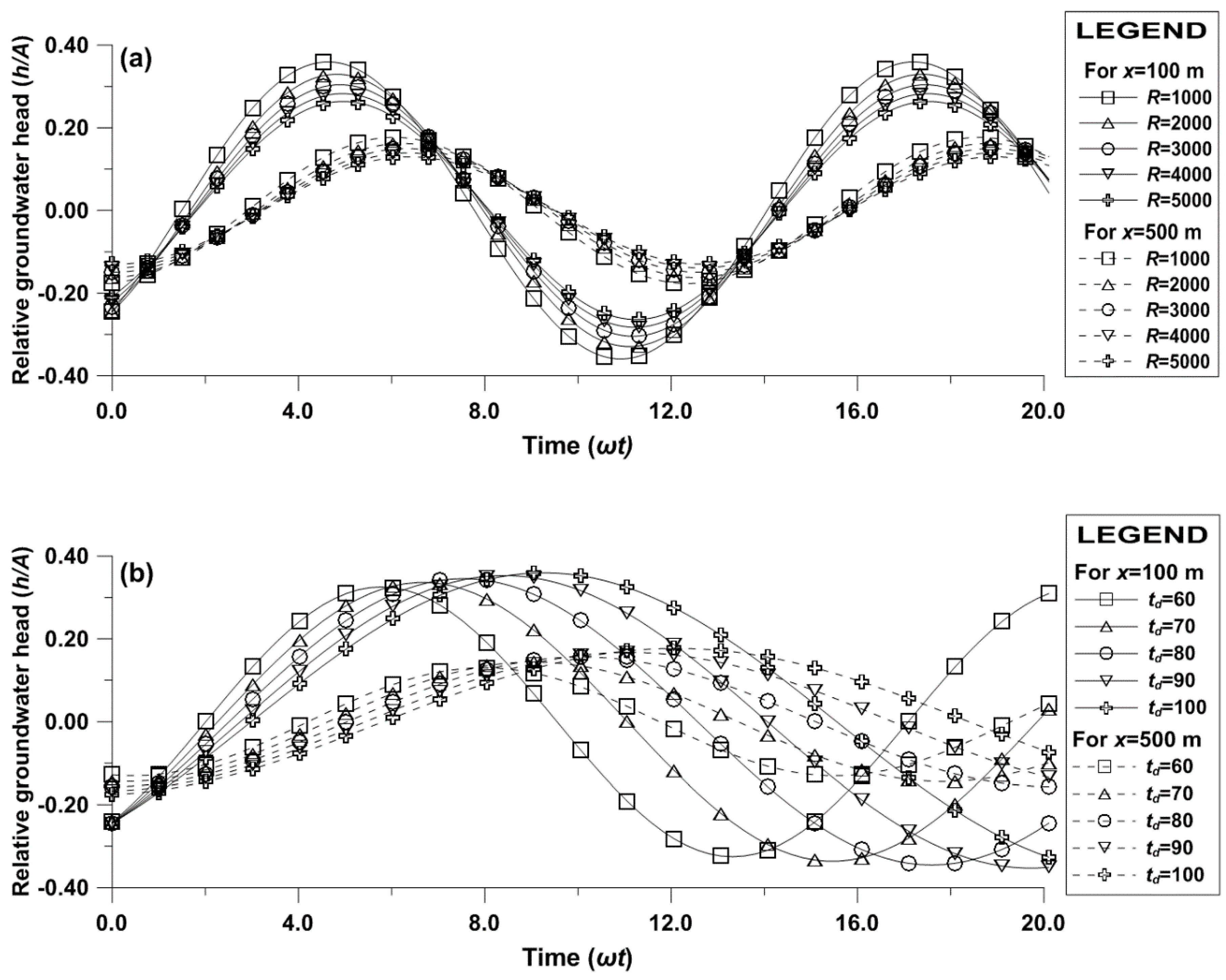
3.2.1. Theoretical Curves Derived from the Analytical Solution

According to the analytical solution, the h/A versus ω t   results for the distances x = 100 and 500 m and for several river resistances (R = 1000, 2000, 3000, 4000, and 5000 m) showed that the h/A values became smaller with increasing river resistance (R) values; moreover, they displayed larger periodicity and lower peaks with increasing x values (Figure 4a). Considering the h/A versus ω t   results for the distances x = 100 and 500 m, for several flood duration times (td = 60, 70, 80, 90, and 100 h), and for a constant R = 1000 m, the h/A values increased with increased flood duration times (td) at a fixed ω t (Figure 4b). This indicates that longer td and larger R values induced lower hydraulic gradient change at a certain distance from the stream–aquifer interface, thus causing a longer lag time for the river-water inflow into the aquifer when the floodwave passed through. On the other hand, the sinusoidal stream variations of the study area were applied with less than one half of the wavelength because of the attenuation effect of floodwave propagation as well as the floodwave impact passing through the channel. Therefore, the actual stream stage did not reach to below that of the initial stage (Figure 4). In this study, the flood duration time (td) was limited within a ωt of 6.28 and the various time scales were all less than π / ω for each of the flood events.

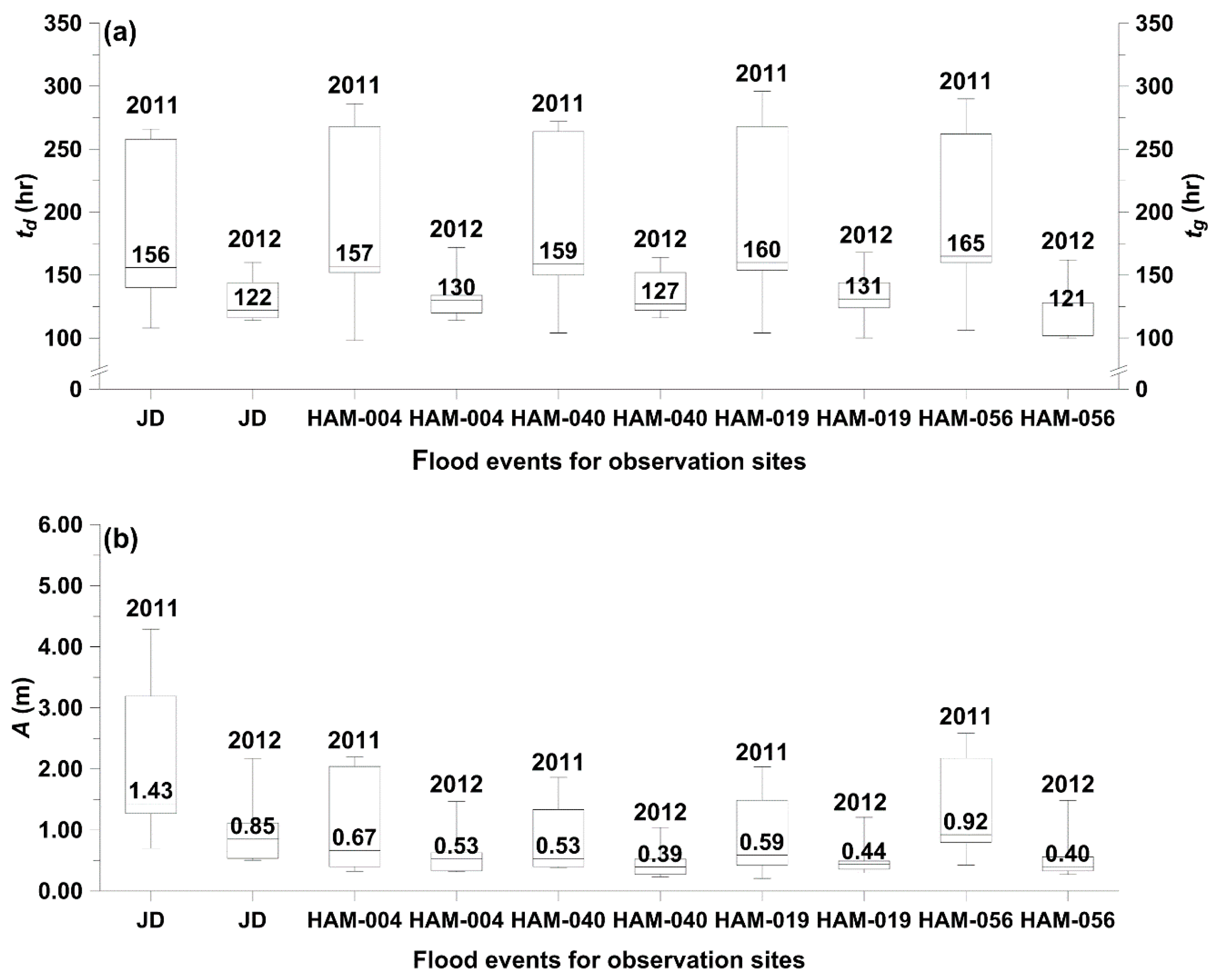
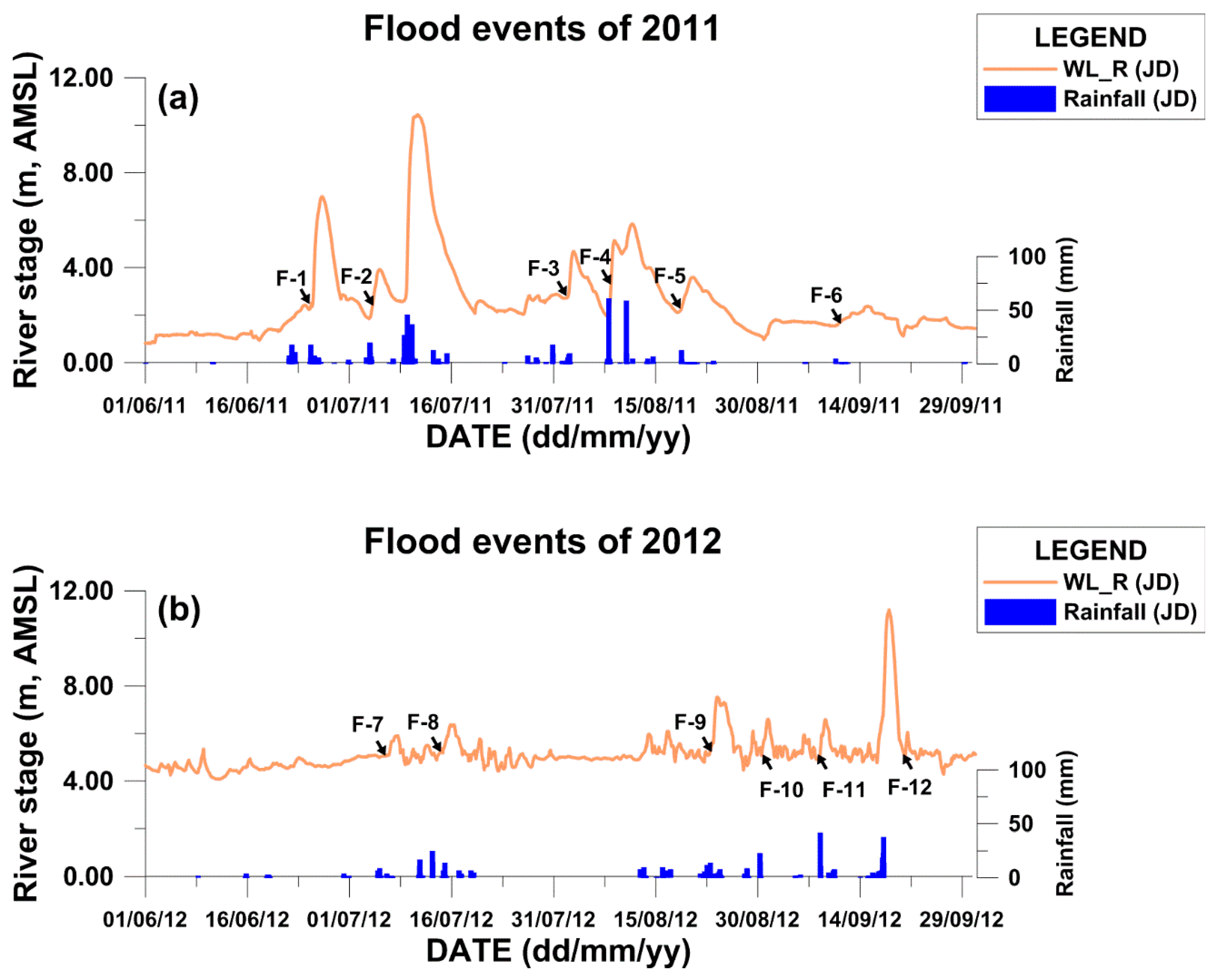
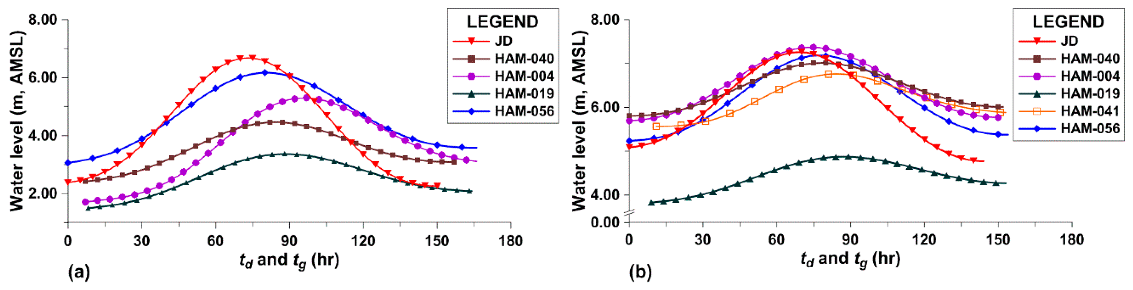
3.2.2. Selection of Flood Events and Changes in Their Characteristics

A total of 12 flood events (F-1 to F-12) were selected for analysis with consideration of the confined boundary conditions, which generally involved unconfined conditions when the water table fluctuations were smaller than 10% of the initial saturated thickness of the aquifer [40]. Figure 5 shows the flood events during the rainy season of 2011 and 2012. Figure 6 displays the flood duration time (td) and induced flood duration time (tg) with amplitude (A) of floodwaves and groundwater fluctuations. The td is the period ranging from the time of the initial river stage to the time that the stage returned to the initial river stage; and the tg corresponds to WL_G. The average of the td and A values from 2011 to 2012 diminished from 181 to 130 h and from 2.05 to 1.01 m, respectively, as a result of the control exerted by the CHRB (Table 3). The highest groundwater fluctuations appeared at the well HAM-056; these values were 2.58 m relative to A = 4.29 m and td = 150 h in 2011, and 1.95 m relative to A = 2.17 m and td = 144 h in 2012. The average of the median td and A values from 2011 to 2012 diminished from 156 to 122 h and from 1.43 to 0.85 m, respectively, which correspond to decreases of 78% and 59%, respectively, compared to the 2011 data. The average of the median tg and A values from 2011 to 2012 also diminished from 160 to 127 h and from 0.68 to 0.44 m, respectively, which correspond to decreases of 79% and 65%, respectively, compared to the 2011 data (Figure 6).
In the rainy season of 2011 (before the construction of the CHRB), based on td and tg as well as A values, the wells far from the CHRB like HAM-056 displayed a stronger response to the Namgang River (a tributary of the Nakdong River) than the wells near the CHRB like HAM-004 (Table 3 and Figure 6). In contrast, in the rainy season of 2012 (after the construction of the CHRB), the majority of the wells in the study area showed a strong response to the Nakdong River (Table 3 and Figure 6). This change indicates that increased river-water storage due to the construction of the CHRB caused the groundwater level to rise around the river, which then reduced the damping effect on floodwaves passing through the aquifer [15,26,27,30,31].
Figure 7 shows the flood peak time (tp) and induced flood peak time (tip). The tp is the time from the initial river stage to the time that the stage reached its peak level, and tip corresponds to WL_G. The ratio of tp to td (or tp/td) represents a key feature of the flood hydrograph [10,22]. Specifically, tp/td and tip/tg values smaller than 0.5 indicate steep hydrographs. The tp values of the floodwave were on average 83 h in 2011 and 57 h in 2012, while tip ranged from an average of 91 h (at HAM-056) to 106 h (at HAM-004) in 2011 and ranged from 62 h (at HAM-004) to 72 h (at HAM-041) in 2012 (Table 3). The average time lag between the groundwater response and the flood peak (tlag) ranged from 8 h (HAM-056) to 23 h (HAM-004) in 2011 and ranged from 5 h (HAM-004) to 13 h (HAM-041) in 2012 (Table 3). The average tip/tg values showed a decreasing tendency with distance from the river in 2011 (Figure 7a,c), but these values showed an increasing trend in 2012 (Figure 7b,c). This change in tendency may reflect the reduction of river flood amplitude caused by the controlled WL_R at the CHRB. In addition, the fluctuations of the WL_Gs and the WL_Rs with the tlag decreased in 2012 (Table 3), which can be explained by enhanced stream–aquifer interactions at the time of flood events F-1 (in 2011) and F-9 (in 2012) (Figure 8a,b).

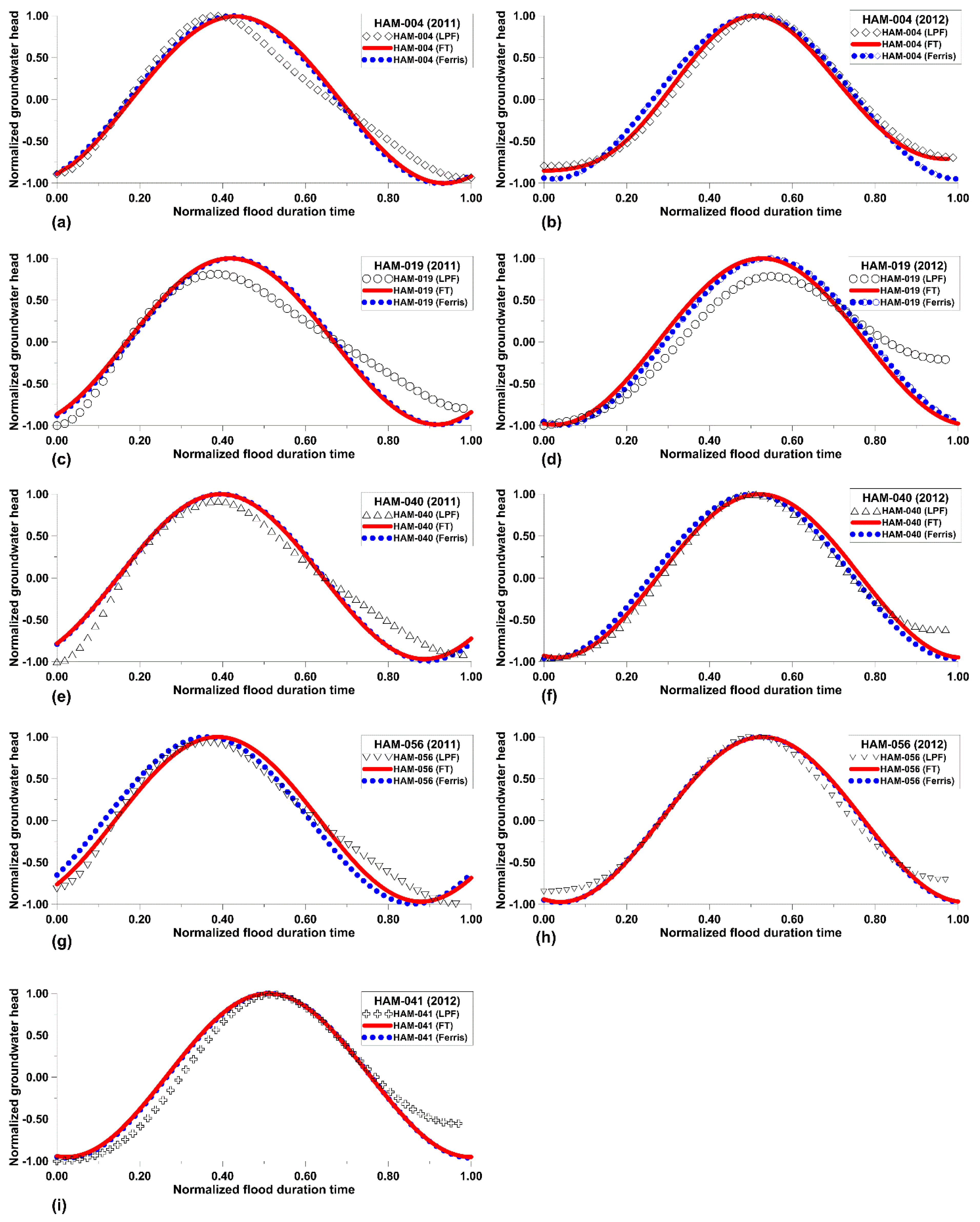
3.2.3. Removal of Noise Effects in Groundwater Level Data

Prior to applying the FRT between WL_R and WL_G, the noise effects of rainfall and pumping were removed from the WL_Gs collected at five monitoring wells (HAM-004, 019, 040, 041, and 056) during the 12 flood events in the rainy seasons of 2011 (F-1 to F-6) and 2012 (F-7 to F-12) (Figure 5). The LPF was performed by cutting off high frequencies among the WL_Gs in order to remove the rainfall and pumping effects with irregular or diurnal cycles. The procedure for determining the cut-off frequency with MATLAB code in this study followed four main steps. These steps included 1) transforming the observed WL_G level data to the frequency domain by using the FFT; 2) analyzing the frequency components and power density and identifying their time scales; 3) selecting the various cut-off frequency bands based on a frequency analysis that compared observed WL_G values by using the inverse FFT, and 4) determining the cut-off frequency with a validation check. The optimal target frequency was determined to be 1.39 × 10⁻⁶ Hz in the range of 1.55 × 10⁻⁸ and 2.78 × 10⁻⁸ Hz with reference to the flood duration time (td). The LPF method effectively corrected irregular changes in groundwater levels, which included effects of barrage operation and agricultural pumping as well as infiltration of rainfall, as shown in the LPF WL_G data at HAM-004 in Figure 9. In this figure, the observed WL_G was well corrected by the LPF as evidenced by the elimination of the effect of the groundwater level decline that occurred on 7 August 2011, due to river-water discharge at the barrage before the beginning of rainfall as well as by the elimination of the effect of rainfall at the flood peak time of 11 August 2011 (Figure 9a). The agricultural pumping effect in early June 2012 and the effect of rainfall at the flood peak time on 10 July 2012, were also removed (Figure 9b).

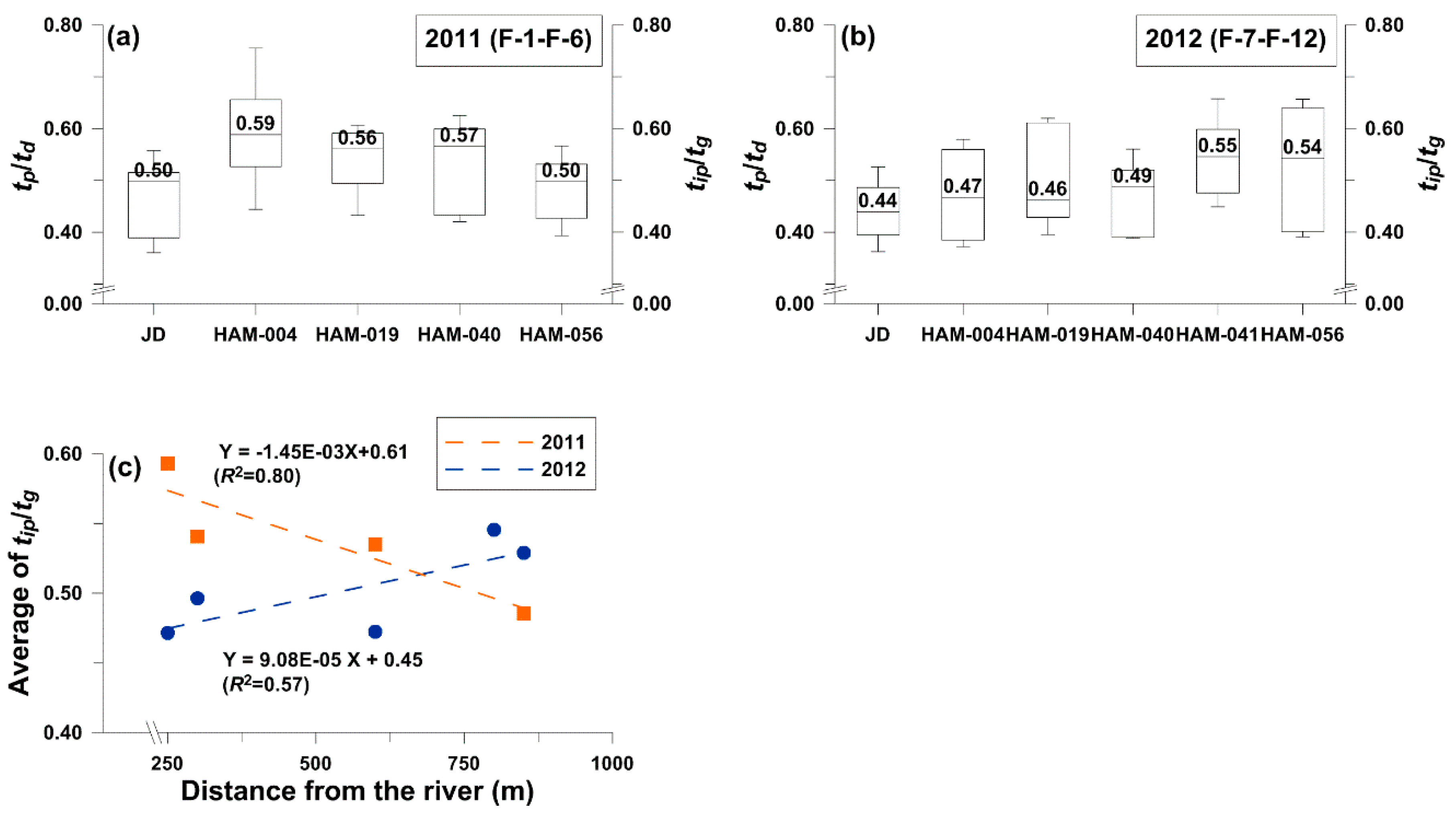
3.2.4. Application of the Analytical Solution for Evaluating Stream–Aquifer Interactions

The 1-D analytical solution was applied to a total of 12 flood events (F-1 to F-12). The 1-D analytical solution in this study assumed confined aquifer conditions because the hydraulic head change was smaller than the initial saturated thickness (<10%) that can be approximated to be associated with the behavior of an unconfined aquifer [9,10,40]. Regarding the assumptions of perpendicular floodwave propagation through the aquifer to the river, and horizontal, uniform groundwater flow [7,10,40], the floodwave through the aquifer in the study area showed approximately perpendicular flow to the river as well as small groundwater level change relative to the initial saturated thickness. Hydraulic conductivity (K) and transmissivity (T) were obtained from the pumping test results (Table 3; [39]); the T values ranged from 1.84 × 10⁻² m2/h (HAM-056) to 4.67 × 10⁻¹ m2/h (HAM-041), and the K values ranged from 8.58 × 10⁻⁸ m/s (HAM-004) to 5.13 × 10⁻⁶ m/s (HAM-041). The hydraulic diffusivity (α) and river resistance (R) were estimated by curve matching to the theoretical curve as shown in Figure 10.
The α values were in the range of 2000 m2/h (HAM-040, F-4) to 85,000 m2/h (HAM-056, F-2) in 2011 and 1640 m2/h (HAM-040, F-10) to 210,000 m2/h (HAM-056, F-9) in 2012 (Figure 11). The estimated R values ranged from 110 m (HAM-004, F-1) to 1940 m (HAM-040, F-5) in 2011 and 50 m (HAM-056, F-10) to 400 m (HAM-056, F-11) in 2012 (Figure 11). The 1-D analytical solution was compared with the method of Ferris [44], which solves the sinusoidal water level variation with a simple harmonic motion but can only consider hydraulic conductivity (K) without R [48,49]. The average values of α calculated by the method of Ferris [44] were similar to those obtained by the 1-D analytical solution with consideration of river resistance (Table 3), i.e., the values calculated by the former method were 88.0% in 2011 and 85.2% in 2012 of the values calculated by the latter method.
The results of this study indicate that the changed R values were due to the alteration of stream-aquifer boundary conditions following the dredging, CHRB construction, and enlargement of the channel width. Besides, the R decrease detected by the 1-D analytical solution can reasonably be attributed to the enhancement of the stream-aquifer interaction in the early period following the completion of the CHRB (Table 3 and Figure 11). However, the increasing trend of α values cannot be understood easily because such hydraulic parameters are generally considered as constant variables, likely due to both the increase of the K (hydraulic conductivity) values and the increased saturated thickness. Additionally, the discrepancy between the theoretical groundwater level and the LPF groundwater level was inferred to be an effect of exaggerated fluctuation due to upstream dam discharge before precipitation as well as the change in the hydrogeological environment since the completion of the CHRB (Figure 10).

4. Conclusions

This study revealed changes in the stream–aquifer interactions during the period shortly after the construction of the Changnyeong–Haman River barrage (CHRB) on the Nakdong River in South Korea. In this work, we estimated the hydraulic diffusivity (α) and river resistance (R) while considering the semipervious layer between the stream and aquifer by using a 1-D analytical solution with Fourier transform (FT) for the sinusoidal stream stage fluctuation case.
The average WL_R increased with an average increase of 1.87 m since the CHRB construction, and the fluctuation of the WL_R decreased with an average decrease of 1.60 m because of the river stage control at the CHRB. The EC_G values also decreased because of the effect of the CHRB construction. The average values of the median of the flood duration time (td) and the amplitude (A) from 2011 to 2012 diminished from 156 to 122 h and from 1.43 to 0.85 m, respectively. In the same manner, the average values of the median of the induced groundwater fluctuation (tg) and A from 2011 to 2012 also diminished from 160 to 127 h and from 0.68 to 0.44 m, respectively. The average values of the ratio of the peak time over the duration time (tip/tg) showed an increasing tendency relative to the distance from the river in 2011, but a decreasing tendency was detected in 2012.
The combined technique of the FFT and LPF prior to the 1-D analytical solution effectively removed noise from the groundwater level data, and this noise included variation due to the river barrage effect and agricultural pumping as well as infiltration of rainfall. The 1-D analytical solution for the 12 flood events (F-1 to F-12) and the WL_G data from five monitoring wells enabled calculations of the hydraulic diffusivity (α) and river resistance (R), and the α values displayed ranges of 2000–180,000 m2/h and 1250–210,000 m2/h in the rainy seasons of 2011 and 2012, respectively; overall, there was an increasing trend. Conversely, the river resistance (R) values displayed ranges of 110–1940 m and 50–400 m in 2011 and 2012, respectively; thus, there was a decreasing trend. The results for the R values indicate that stream–aquifer interactions were enhanced by dredging, water storage increases in the CHRB, and increases in the groundwater level adjacent to the river as a result of the effect of the CHRB construction. These findings also indicate that R values can function as useful indicators for estimating hydrogeological environment change as well as changes in stream–aquifer interactions adjacent to rivers influenced by river barrage construction.
Even though some limitations were encountered, the 1-D analytical solution was found to be suitable for the study area and useful for the analysis of floodwaves through the aquifer, which occurred nearly perpendicularly to the river, as well as for the small groundwater level change that took place relative to the initial saturated thickness (<10%). However, caution is needed in that the elimination of noise effects from the groundwater level data can greatly influence the α and R values when applying the 1-D analytical solution with FT. Therefore, proper selection of flood events before application of the 1-D analytical solution is highly recommended for determining reliable α and R values.

Acknowledgments

This study was supported by the Basic Science Research Program through the National Research Foundation of Korea (NRF), which is funded by the Ministry of Education (NRF-2013R1A1A2058186) and also supported by Korea Ministry of Environment (MOE) as “Korea-CO2 Storage Environmental Management (K-COSEM) Research Program”.

Author Contributions

This manuscript was mainly written by both Yun-Yeong Oh and Se-Yeong Hamm with partial contributions from the other co-authors. The main concept of the manuscript was developed by Yun-Yeong Oh and Se-Yeong Hamm, and they collected and analyzed the data. Kyoochul Ha reviewed the 1-D analytical equation data; Il-Moon Chung interpreted the flood hydrographs; and Heesung Yoon reviewed the low-pass filtering results.

Conflicts of Interest

The authors declare no conflict of interest.

References

  1. Illangasekare, T.; Morel-Seytoux, H.J. Stream-aquifer influence coefficients as tools for simulation and management. Water Resour. Res. 1982, 18, 168–176. [Google Scholar] [CrossRef]
  2. Sophocleous, M.; Koussis, A.; Martin, J.L.; Perkins, S.P. Evaluation of simplified stream-aquifer depletion models for water rights administration. Groundwater 1995, 33, 579–588. [Google Scholar] [CrossRef]
  3. Ray, C.; Soong, T.W.; Lian, Y.Q.; Roadcap, G.S. Effect of flood-induced chemical load on filtrate quality at bank filtration sites. J. Hydrol. 2002, 266, 235–258. [Google Scholar] [CrossRef]
  4. Chen, X.; Chen, X. Stream water infiltration, bank storage, and storage zone changes due to stream-stage fluctuations. J. Hydrol. 2003, 280, 246–264. [Google Scholar] [CrossRef]
  5. McCallum, J.L.; Cook, P.G.; Brunner, P.; Berhane, D. Solute dynamics during bank storage flows and implications for chemical base flow separation. Water Resour. Res. 2010, 46. [Google Scholar] [CrossRef]
  6. Pinder, G.F.; Bredehoeft, J.D.; Cooper, H.H. Determination of aquifer diffusivity from aquifer response to fluctuations in river stage. Water Resour. Res. 1969, 5, 850–855. [Google Scholar] [CrossRef]
  7. Reynolds, R.J. Diffusivity of glacial-outwash aquifer by the floodwave-response technique. Groundwater 1987, 25, 290–299. [Google Scholar] [CrossRef]
  8. Barlow, P.M.; DeSimone, L.A.; Moench, A.F. Aquifer response to stream-stage and recharge variations. II. Convolution method and applications. J. Hydrol. 2000, 230, 211–229. [Google Scholar] [CrossRef]
  9. Jha, M.K.; Jayalekshmi, K.; Machiwal, D.; Kamii, Y.; Chikamori, K. Determination of hydraulic parameters of an unconfined alluvial aquifer by the floodwave-response technique. Hydrogeol. J. 2004, 12, 628–642. [Google Scholar] [CrossRef]
  10. Ha, K.; Koh, D.C.; Yum, B.W.; Lee, K.K. Estimation of layered aquifer diffusivity and river resistance using flood wave response model. J. Hydrol. 2007, 337, 284–293. [Google Scholar] [CrossRef]
  11. Jung, M.; Burt, T.P.; Bates, P.D. Toward a conceptual model of floodplain water table response. Water Resour. Res. 2004, 40. [Google Scholar] [CrossRef] [Green Version]
  12. Hantush, M.M. Modeling stream–aquifer interactions with linear response functions. J. Hydrol. 2005, 311, 59–79. [Google Scholar] [CrossRef]
  13. Welch, C.; Harrington, G.A.; Leblanc, M.; Batlle-Aguilar, J.; Cook, P.G. Relative rates of solute and pressure propagation into heterogeneous alluvial aquifers following river flow events. J. Hydrol. 2014, 511, 891–903. [Google Scholar] [CrossRef]
  14. Welch, C.; Cook, P.G.; Harrington, G.A.; Robinson, N.I. Propagation of solutes and pressure into aquifers following river stage rise. Water Resour. Res. 2013, 49, 5246–5259. [Google Scholar] [CrossRef]
  15. Lewandowski, J.; Lischeid, G.; Nützmann, G. Drivers of water level fluctuations and hydrological exchange between groundwater and surface water at the lowland River Spree (Germany): Field study and statistical analyses. Hydrol. Process. 2009, 23, 2117–2128. [Google Scholar] [CrossRef]
  16. Burt, T.P.; Bates, P.D.; Stewart, M.D.; Claxton, A.J.; Anderson, M.G.; Price, D.A. Water table fluctuations within the floodplain of the River Severn, England. J. Hydrol. 2002, 262, 1–20. [Google Scholar] [CrossRef]
  17. Gillham, R.W. The capillary fringe and its effect on water-table response. J. Hydrol. 1984, 67, 307–324. [Google Scholar] [CrossRef]
  18. Kondolf, G.M. Hungry water: effects of dams and gravel mining on river channels. Environ. Manag. 1997, 21, 533–551. [Google Scholar] [CrossRef]
  19. Sawyer, A.H.; Cardenas, M.B.; Bomar, A.; Mackey, M. Impact of dam operations on hyporheic exchange in the riparian zone of a regulated river. Hydrol. Process. 2009, 23, 2129–2137. [Google Scholar] [CrossRef]
  20. Francis, B.A.; Francis, L.K.; Cardenas, M.B. Water table dynamics and groundwater–surface water interaction during filling and draining of a large fluvial island due to dam-induced river stage fluctuations. Water Resour. Res. 2010, 46. [Google Scholar] [CrossRef]
  21. Singh, S.K. Aquifer response to sinusoidal or arbitrary stage of semipervious stream. J. Hydraul. Eng. 2004, 130, 1108–1118. [Google Scholar] [CrossRef]
  22. Hall, F.R.; Moench, A.F. Application of the convolution equation to stream-aquifer relationships. Water Resour. Res. 1972, 8, 487–493. [Google Scholar] [CrossRef]
  23. Carslaw, H.S.; Jaeger, J.C. Conduction of Heat in Solids, 2nd ed.; Clarendon Press: Oxford, UK, 1959; pp. 50–127. [Google Scholar]
  24. Bruggeman, G.A. One-dimensional groundwater flow: Orientation table BI. Dev. Water Sci. 1999, 46, 77–78. [Google Scholar]
  25. Dong, L.; Cheng, D.; Liu, J.; Zhang, P.; Ding, W. Analytical analysis of groundwater responses to estuarine and oceanic water stage variations using superposition principle. J. Hydraul. Eng. 2016, 21, 04015046. [Google Scholar] [CrossRef]
  26. Cloutier, C.A.; Buffin-Bélanger, T.; Larocque, M. Controls of groundwater floodwave propagation in a gravelly floodplain. J. Hydrol. 2014, 511, 423–431. [Google Scholar] [CrossRef]
  27. García-Gil, A.; Vázquez-Suñé, E.; Sánchez-Navarro, J.Á.; Lázaro, J.M.; Alcaraz, M. The propagation of complex flood-induced head wavefronts through a heterogeneous alluvial aquifer and its applicability in groundwater flood risk management. J. Hydrol. 2015, 527, 402–419. [Google Scholar] [CrossRef]
  28. Zlotnik, V.A.; Huang, H. Effect of shallow penetration and streambed sediments on aquifer response to stream stage fluctuations (analytical model). Groundwater 1999, 37, 599–605. [Google Scholar] [CrossRef]
  29. Singh, V.P. Is hydrology kinematic? Hydrol. Process. 2002, 16, 667–716. [Google Scholar] [CrossRef]
  30. Vidon, P. Towards a better understanding of riparian zone water table response to precipitation: Surface water infiltration, hillslope contribution or pressure wave processes? Hydrol. Process. 2012, 26, 3207–3215. [Google Scholar] [CrossRef]
  31. Vekerdy, Z.; Meijerink, A.M.J. Statistical and analytical study of the propagation of flood-induced groundwater rise in an alluvial aquifer. J. Hydrol. 1998, 205, 112–125. [Google Scholar] [CrossRef]
  32. Barlow, J.R.; Coupe, R.H. Use of heat to estimate streambed fluxes during extreme hydrologic events. Water Resour. Res. 2009, 45, 1–10. [Google Scholar] [CrossRef]
  33. Sophocleous, M.A. Stream-floodwave propagation through the Great Bend alluvial aquifer, Kansas: Field measurements and numerical simulations. J. Hydrol. 1991, 124, 207–228. [Google Scholar] [CrossRef]
  34. Ministry of Land, Transportation, and Maritime Affairs (MLTM). The Detail Design of Development of Residential Sites for Nakdong River 18 District; MLTM: Seoul, Korea, 2009.
  35. Ministry of Land, Infrastructure, and Transport (MOLIT). Korea Annual Hydrological Report 2013; MOLIT: Seoul, Korea, 2013.
  36. National Climate Data Service System (NCDSS). Available online: http://sts.kma.go.kr/eng/jsp/home/contents/main/main.do (accessed on 29 September 2015).
  37. Choi, S.H.; Lyeo, S.C. National Geological Survey of Korea; Geological map of Namji Sheet (1:50000); National Geological Survey of Korea: Seoul, Korea, 1972; Sheet-6820-II. [Google Scholar]
  38. Kim, G.-B.; Cha, E.-J.; Jeong, H.-G.; Shin, K.-H. Comparison of time series of alluvial groundwater levels before and after barrage construction on the lower Nakdong River. J. Eng. Geol. 2013, 23, 105–115. (In Korean) [Google Scholar] [CrossRef]
  39. Hydronet Limited (Hydronet). The Report for the Installation of the Groundwater Observation Equipment; Hydronet Limited: Seoul, Korea, 2012; pp. 1–311. [Google Scholar]
  40. Spanoudaki, K.; Nanou-Giannarou, A.; Paschalinos, Y.; Memos, C.D.; Atamou, A.I. Analytical solutions to the stream-aquifer interaction problem: A critical review. Global NEST J. 2010, 12, 126–139. [Google Scholar]
  41. Hantush, M.S. Wells near streams with semipervious beds. J. Geophys. Res. 1965, 70, 2829–2838. [Google Scholar] [CrossRef]
  42. Cooper, H.H.; Rorabaugh, M.I. Ground-water Movements and Bank Storage Due to Flood Stages in Surface Streams; U.S. Government Printing Office: Washington, DC, USA, 1963; pp. 343–366.
  43. Hantush, M.S. Discussion of paper by P.P. Rowe, An equation for estimating transmissibility and coefficient of storage from river-level fluctuations. J. Geophys. Res. 1961, 66, 1310–1311. [Google Scholar] [CrossRef]
  44. Ferris, J.G. Cyclic fluctuations of water level as a basis for determining aquifer transmissibility. Assemblee Generale Bruxelles Ass. Int. Hydrol. Sci. 1951, 2, 148–155. [Google Scholar]
  45. Bentall, R. Methods of Determining Permeability, Transmissibility and Drawdown; USGS Water Supply Paper 1536-I; United States Government Printing Office: Washington, DC, USA, 1964; p. 99.
  46. Spongberg, M.E. Spectral analysis of base flow separation with digital filters. Water Resour. Res. 2000, 36, 745–752. [Google Scholar] [CrossRef]
  47. Walker, J.S. Fast Fourier Transforms, 2nd ed.; CRC Press: Boca Raton, FL, USA, 1996; pp. 58–76. [Google Scholar]
  48. Jacob, C.E. Flow of Groundwater in Engineering Hydraulics; Rouse, H., Ed.; John Wiley: New York, NY, USA, 1950; pp. 321–386. [Google Scholar]
  49. Carr, P.A.; Van Der Kamp, G.S. Determining aquifer characteristics by the tidal method. Water Resour. Res. 1969, 5, 1023–1031. [Google Scholar] [CrossRef]
Figure 1. Study area.
Water 08 00137 g001
Figure 2. Schematic cross-section of A-Aʹ (modified from [36]).
Water 08 00137 g002
Figure 3. Temporal variation of the (a) water level and (b) electrical conductivity in the study area. NG_R, YS_S, and GR_S represent the Namgang River area, Yeongsan Stream area, and Gwangryeo Stream area, respectively.
Water 08 00137 g003
Figure 4. Dimensionless groundwater head (h/A) for dimensionless time ( ω t ) and distance from the river−aquifer interface according to (a) river resistance (R) and (b) flood duration time (td).
Water 08 00137 g004
Figure 5. Flood events (a) F-1 to F-6 of 2011 and (b) F-7 to F-12 of 2012 during the rainy season.
Water 08 00137 g005
Figure 6. Flood duration time (td) in JD and duration time of induced groundwater fluctuation (tg) in observation wells (HAM-004, 040, 019, 056) along with amplitude (A) values for floodwave and groundwater fluctuations during flood events F-1 to F-6 in 2011 and F-7 to F-12 in 2012; (a) td versus tg, and (b) A, respectively.
Water 08 00137 g006
Figure 7. Flood duration time of groundwater levels (WL_Gs) for the flood events in 2011 and 2012; (a) tp/td (in JD) and tip/tg (in observation wells) in 2011; (b) tp/td and tip/tg in 2012; and (c) average of tip/tg versus distance from the river in 2011 and 2012.
Water 08 00137 g007
Figure 8. Water level versus td and tg for (a) the F-1 event in 2011 and (b) the F-9 event in 2012.
Water 08 00137 g008
Figure 9. Example of observed (OBS) and low-pass filtered (LPF) groundwater level data at HAM-004 during the rainy season of (a) 2011 and (b) 2012.
Water 08 00137 g009
Figure 10. Example of normalized filtered groundwater level (WL_G) data (i.e., low-pass filtered (LPF) data) versus normalized tg by the Fourier transform (FT) solution and Ferris (1951) [44] solution for flood events of F-4 (2011) and F-9 (2012); (a) HAM-004 in 2011; (b) HAM-004 in 2012; (c) HAM-019 in 2011; (d) HAM-019 in 2012; (e) HAM-040 in 2011; (f) HAM-040 in 2012; (g) HAM-056 in 2011; (h) HAM-056 in 2012; and (i) HAM-041 in 2012.
Water 08 00137 g010
Figure 11. Changes in hydraulic diffusivity (α) and river resistance (R) derived through use of the Fourier transform method. The numbers along the x-axis indicate the flood events, which are shown in order. (a) HAM-004; (b) HAM-040; (c) HAM-019; (d) HAM-056; and (e) HAM-041.
Water 08 00137 g011
Table 1. Measurement periods and data for analyses.
DataUnitLocationObservation Period
RainfallmmYeongsan (in YS_S), Jindong (in GR_S), and Georyonggang (in NG_R) rainfall gauge stationsJune 2011–February 2013
WL_Rm (AMSL)Deongnam (in YS_S), Jingdong (in GR_S), and Georyonggang (in NG_R) gauge stations
Electrical conductivity of river water (EC_R)µS/cmChilseo purification plant (with the Jingdong gauge station)July 2012–February 2013
Groundwater level (WL_G) and Electrical conductivity (EC_G)m (AMSL) and µS/cmHAM-004, 005, 007, 008, 010, 013, 019, 022 (in YS_S), 038, 040, 042, 043, 046 (in GR_S), 056, 057, 059 (in NG_R)June 2011–February 2013
HAM-014, 015, 021, 023, 035 (in YS_S), 045, 047, 048 (in GR_S), 060, 061, 062, 063, 064, 065 (in NG_R)June 2012–February 2013
Table 2. Variation of average groundwater level and electrical conductivity with rainfall.
Year/SeasonBefore the River BarrageAfter the River Barrage
20112012
Rainy (June–September)Dry (November–Februaty)Rainy (June–September)Dry (November–February)
Rainfall (mm)1018125862175
WL_R (m, AMSL)2.583.295.154.46
Fluctuation of WL_R (max–min. m)9.502.297.121.48
WL_G (m, AMSL)4.645.035.404.88
Average differences of WL_R (m)1.87
Fluctuation of WL_G (m) (max–min, m)12.308.1513.759.74
Average differences of WL_R fluctuation (m)1.60
EC_R (µS/cm)--370262
Fluctuation of EC_R (max–min, µS/cm)--549322
EC_G (µS/cm)675670680650
Fluctuation of EC_G (max–min, µS/cm)1404235117091544
Table 3. Average values of estimated hydraulic parameters (FT: 1-D analytical solution derived by the Fourier transform).
Observation PointFactors of Observation PointsFlood Events (F-1 to F-12) in June–September
F-1 to F-6 in 2011F-7 to F-12 in 2012
FTFerris (1951) [44]FTFerris (1951) [44]
Jindong (JD)td (h)181130
tp (h)8357
A (m)2.050.54
HAM-004tg (h)186133
tip (h)/tlag (h)106/2362/5
A (m)1.050.63
x (m)300
T (m2/h)/K (m/s)1.22 × 10−2/8.68 × 10−8
α (m2/h)5400398021,85016,850
R (m)335-88-
HAM-019tg (h)190133
tip (h)/tlag (h)101/1865/9
A (m)0.840.48
x (m)600
T (m2/h)/K (m/s)3.73 × 10−1/3.91 × 10−6
α (m2/h)11,250930022,71719,850
R (m)420-125-
HAM-040tg (hr)185135
tip (h)/tlag (h)97/1463/6
A (m)0.890.54
x (m)250
T (m2/h)/K (m/s)4.52 × 10−2/4.18 × 10−7
α (m2/h)3333204569835357
R (m)975-108-
HAM-041tg (h)-128
tip (h)/tlag (h)-70/13
A (m)-0.52
x (m)800
T (m2/h)/K (m/s)4.67 × 10−1/5.13 × 10−6
α (m2/h)--52,53346,350
R (m)--138-
HAM-056tg (h)191122
tip (h)/tlag (h)91/863/7
A (m)1.300.57
x (m)850
T (m2/h)/K (m/s)1.84 × 10−2/1.50 × 10−7
α (m2/h)74,16767,566132,667114,917
R (m)363-163-

