Using Endmember Ion Fingerprinting for Source Apportionment of River Hydrochemistry in the Huxi Catchment, Taihu Lake Basin

Abstract

Understanding the hydrochemical characteristics and formation mechanisms of rivers in the Huxi Catchment is essential for water resource conservation, as these rivers serve as the primary water source for Taihu Lake. A total of 14 surface water samples were collected from the rivers in Huxi catchment, and the concentrations of seven major ions—namely, ${\mathrm{N}\mathrm{a}}^{+}$, ${\mathrm{K}}^{+}$, ${\mathrm{C}\mathrm{a}}^{2+}$, ${\mathrm{M}\mathrm{g}}^{2+}$, ${\mathrm{C}\mathrm{l}}^{-}$, ${\mathrm{S}\mathrm{O}}_4^{2-}$, and ${\mathrm{H}\mathrm{C}\mathrm{O}}_3^{-}$—were determined. Positive Matrix Factorization (PMF), Absolute Principal Component Score–Multiple Linear Regression (APCS-MLR), and the Principal Component Analysis-based Endmember Mixing Model (PCA-EMM) were employed to quantify the contributions of anthropogenic activities. While APCS-MLR can only identify the impacts of human activities, PMF and PCA-EMM can further distinguish between agricultural activities and wastewater discharge. Significant positive correlations were observed between the PMF and PCA-EMM results, but PMF overestimated the contribution of anthropogenic impacts. PCA-EMM showed that the natural background accounted for 63%, while human activities contributed 37% (domestic sewage 23%, agricultural activities 14%). By integrating ion composition data from representative sources, PCA-EMM overcomes the limitations of traditional methods that lack source verification and provides robust methodological support for the source apportionment of water chemistry.

1. Introduction

Freshwater salinization has emerged as a pressing global environmental issue, particularly in regions experiencing intensive human activity [1,2]. The progressive increase in freshwater salinity poses significant threats to aquatic ecosystems, including shifts in species composition, deterioration of water quality, and potential risks to drinking water safety and agricultural irrigation [3,4]. As one of the most developed and densely populated regions in China, the Taihu Lake Basin faces intense anthropogenic pressures, including extensive agricultural activity and rapid urbanization [5], which underscores the urgent need for research on surface water salinity in this basin.

The water salinity of surface water is primarily due to the presence of cations, such as ${\mathrm{Ca}}^{2+}$, ${\mathrm{Mg}}^{2+}$, ${\mathrm{Na}}^{+}$, ${\mathrm{K}}^{+}$, and anions including ${\mathrm{HCO}}_3^{-}$, ${\mathrm{SO}}_4^{2-}$, and ${\mathrm{Cl}}^{-}$. Under natural conditions, these ions originate mainly from rock weathering processes [6]; however, increasing anthropogenic inputs—such as wastewater discharge and agricultural runoff—have significantly altered the ionic concentrations [6], leading to elevated concentrations of specific ions, most notably ${\mathrm{Na}}^{+}$ and ${\mathrm{Cl}}^{-}$. As reported by Dai et al., influenced by sewage discharge, the dominant anion in Taihu Lake has shifted from ${\mathrm{HCO}}_3^{-}$ to ${\mathrm{Cl}}^{-}$, while ${\mathrm{Na}}^{+}$ has surpassed ${\mathrm{Ca}}^{2+}$ to become the dominant cation [7]. In addition, approximately 100,000 tons of potassium fertilizer (KCl) and 250,000 tons of phosphate fertilizer (calcium superphosphate) are applied annually to farmland in the Taihu Lake basin [8]. While potassium and phosphorus are absorbed by plants, ${\mathrm{Cl}}^{-}$ and ${\mathrm{Ca}}^{2+}$ undergo limited plant uptake and are subsequently transported into surface water bodies via rainfall or irrigation [9]. Consequently, from the 1950s to 2010s, the concentrations of major cations and anions in Taihu Lake increased significantly, with Cl⁻ and Na⁺ increasing by 400% and 300%, respectively, and Ca²⁺ and Mg²⁺ increasing by 200% and 90%, respectively [10]. Human activities not only lead to the salinization of surface water but also significantly alter the ion ratios of water chemistry. Specifically, the (Ca²⁺ + Mg²⁺)/${\mathrm{HCO}}_3^{-}$ and Cl⁻/Na⁺ ratios have significantly increased, whereas the ${\mathrm{SO}}_4^{2-}$/Cl⁻ ratio has significantly decreased [11], indicating human intervention in the lake’s hydrochemistry.

Given the diversity of ion sources, accurately identifying and quantifying them are essential to understand the mechanisms driving river salinization and to develop effective control strategies [2]. Currently, the main methodologies for tracing ion sources are receptor models, such as Absolute Principal Component Score–Multiple Linear Regression (APCS-MLR) and Positive Matrix Factorization (PMF) [12]. The source apportionment by APCS-MLR is based on the dimension reduction by PCA [13]. APCS–MLR source apportionment identified four major sources—natural (53.34%), agricultural (22.71%), ion-exchange (4.79%), and an unknown anthropogenic source (19.14%)—in the Nansi Lake, Northern China. Unlike APCS-MLR, PMF decomposes the observed data matrix into source contributions and source profiles matrix under a non-negative constraint [14]. Using PMF, Zheng et al. showed that Aixi Lake, Eastern China, contained non-point source pollution (contributed 32.0%) and the results of biogeochemical processes (contributed 28.4%) [15]. However, both the APCS-MLR and PMF models lack the empirical chemical characterization of source profiles, leaving a critical gap in the source apportionment by receptor model [16].

The Huxi Catchment contributes 75% of the total inflow volume of Taihu Lake, Jiangsu and Zhejiang Provinces, Eastern China. This area is characterized by three typical features: flat topography underlain by carbonate rocks; a dense river network covering 9% of the total area; and substantial human activity, with farmland and construction land accounting for 67% and 16% of land use, respectively. In this study, we analyzed the ionic concentrations in river water and representative sources (domestic sewage and agricultural soil solutions) in the Huxi Catchment. APCS-MLR and PMF were applied to apportion the sources of these ions. Furthermore, we developed a principal component analysis-based endmember mixing model (PCA-EMM) that integrated empirical data from representative sources to quantify the impacts of sewage discharge and agricultural activities on the river hydrochemistry. The aims of this study are to (1) characterize the spatial variations in river hydrochemistry along an anthropogenic impact gradient from upstream to downstream within the Huxi Catchment, (2) apportion the sources of river hydrochemistry by incorporating empirical data from representative sources, and (3) compare the performance of different models (APCS-MLR, PMF, and PCA-EMM) in source apportionment.

2. Materials and Methods

2.1. Study Area

The Huxi catchment is located in the upper reaches of the Taihu Lake Basin, spanning from 119°03′ E to 120°10′ E and 31°06′ N to 32°15′ N, with a total area of 7896 km². Climatically, the catchment experiences a subtropical monsoon climate, with an average annual rainfall of approximately 1213 mm. Geologically, the catchment is dominated by carbonate rocks, which strongly influences its hydrochemistry [17]. Human activity in the catchment is also highly intensive, with farmland and construction land accounting for 67% and 16%, respectively, while forests and open water bodies constitute the remaining 17%. The predominance of agricultural and urban land use, coupled with the limited extent of natural landscapes, indicates that anthropogenic inputs likely constitute the dominant source of solutes in the river system. This land use configuration renders the Huxi catchment an ideal setting for investigating the impacts of human activity on riverine hydrochemistry.

2.2. Sample Collection

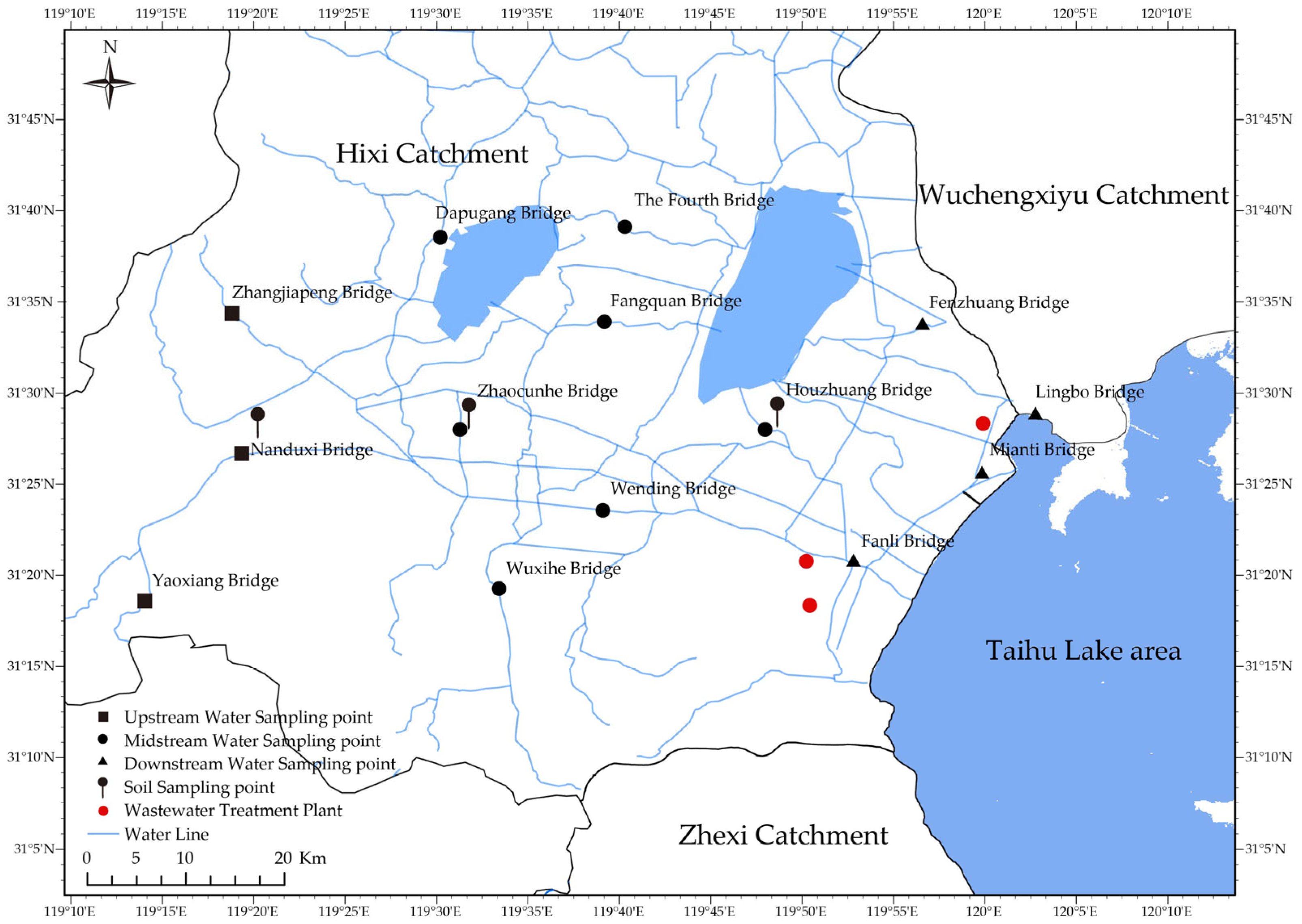
In March 2025, 14 water samples were collected from major rivers in the Huxi Catchment (Figure 1) during the dry season, when water salinity peaks for the year, which provides the most valuable conditions for source apportionment [18]. These sampling points were selected based on two principles: (1) prioritizing easily accessible locations, such as river-crossing bridges; and (2) ensuring an even distribution from upstream to downstream to capture the gradient of anthropogenic impact on the hydrochemistry. In addition, three water samples were collected from the wastewater treatment plant (Figure 1).

The water samples were collected using acrylic water samplers at a depth of 20 cm below the water surface. Prior to collection, the sampling bags were rinsed twice with sampling water to minimize container-induced contamination. All samples were immediately filtered on-site through 0.45 μm membrane filters. The aliquots intended for cation analysis were acidified to pH < 2 using ultrapure nitric acid, while the aliquots for anion analysis were stored unacidified. The samples were sealed immediately, transported to the laboratory within 12 h, stored at 4 °C, and analyzed for ion concentrations within 48 h.

Moreover, representative farmland soil samples were also collected near upstream (Nanduxi Bridge) and midstream (Zhaocunhe Bridge and Houzhuang Bridge) sampling sites (Figure 1). At each site, five sub-samples were collected using an S-shaped sampling pattern, with adjacent sub-samples spaced more than 20 m apart. Topsoil (0–10 cm depth) was collected using a soil drill. The five sub-samples from each site were mixed uniformly, naturally air-dried, ground, and sieved through a 2 mm mesh for the subsequent determination of the water-soluble ion content.

2.3. Analytical Testing

All water quality analyses were performed in accordance with the procedures described in the Standard Methods for the Examination of Water and Wastewater, 24th Edition (APHA, AWWA, WEF, 2023) [19]. Specifically, the total hardness (the sum of calcium and magnesium) in the water samples was determined via EDTA titration (Standard Method 2340-Hardness). Concentrations of ${\mathrm{Ca}}^{2+}$, ${\mathrm{Na}}^{+}$, and ${\mathrm{K}}^{+}$ were measured using a flame photometer (Standard Method 3500-Ca, Na and K) [19]. The ${\mathrm{Mg}}^{2+}$ concentration was then calculated by subtracting the ${\mathrm{Ca}}^{2+}$ concentration from the total hardness (Standard Method 3500-Mg). The Cl⁻ concentration was determined via the argentometric method (Standard Method 4500-Cl⁻), the ${\mathrm{SO}}_4^{2-}$ concentration was measured via the turbidimetric method (Standard Method 4500-${\mathrm{SO}}_4^{2-}$), and the ${\mathrm{HCO}}_3^{-}$ concentration was quantified via the titration method (Standard Method 2320-Alkalinity).

The charge balance error (CBE) was calculated for each sample using the following formula: CBE (%) = (Σcations − Σanions)/(Σcations + Σanions) × 100, where Σcations and Σanions represent the sum of the major cations (${\mathrm{Ca}}^{2+}$, ${\mathrm{M}\mathrm{g}}^{2+}$, ${\mathrm{Na}}^{+}$, and ${\mathrm{K}}^{+}$) and anions (Cl⁻, ${\mathrm{SO}}_4^{2-}$, and ${\mathrm{HCO}}_3^{-}$) in milliequivalents per liter (meq/L), respectively. All samples analyzed in this study exhibited CBE values within ±1%, which is within the acceptable range for hydrochemical studies, thereby validating the analytical precision and data reliability.

The total dissolved solids were calculated as the sum of ${\mathrm{Ca}}^{2+}$, ${\mathrm{Na}}^{+}$, ${\mathrm{K}}^{+}$, Cl⁻, ${\mathrm{SO}}_4^{2-}$, and 1/2${\mathrm{HCO}}_3^{-}$. To determine the water-soluble ions in the soil samples, sieved soil samples were shaken with deionized water at a soil-to-water ratio of 1:10 for 3 min. The resulting mixtures were filtered through 0.45 μm membrane filters to obtain soil extracts. The concentrations of the target ions in the extracts were then measured using the methods described above.

2.4. Data Analysis

Positive matrix factorization (PMF) was performed, according to the United States Environmental Protection Agency [20,21]. PMF approximately decomposes a non-negative original data matrix V (m × n) into the product of two low-dimensional and non-negative matrices: V ≈ W × H. W (m × r) is the source profile matrix, and matrix H (r × n) is the source contribution matrix. Herein, m denotes the number of samples, n represents the number of measured environmental parameters, and r stands for the number of identified sources. An alternating updating algorithm is adopted to iteratively minimize the difference between V and W × H [22]. The APCS-MLR model combines multiple linear regression (MLR) and the absolute principal component score (APCS) from PCA [23]. The source contribution was calculated as follows [24]. The contribution of the k-th source to the j-th ion in the i-th sampling site is defined as ${\mathrm{C}\mathrm{R}}_{\mathrm{ikj}} = |{\mathsf{\beta }}_{\mathrm{jk}} \text{×} {\mathrm{APCS}}_{\mathrm{ik}}|/({|\mathrm{b}}_{\mathrm{jk}}|+ {\sum }_{\mathrm{k}=1}^{\mathrm{n}}\left(\right|{\mathsf{\beta }}_{\mathrm{jk}} \text{×} {\mathrm{APCS}}_{\mathrm{kij}}\left|\right))$. Then, the average contribution of the k-th source to all ions in the i-th sampling site is calculated as ${\mathrm{C}\mathrm{R}}_{\mathrm{ik}}={\sum }_{\mathrm{j}=1}^{\mathrm{p}}\left({\mathrm{CR}}_{\mathrm{ikj}}\right)/\mathrm{p}$. Herein, ${\mathrm{b}}_{\mathrm{j}0}$ and ${\mathsf{\beta }}_{\mathrm{jk}}$ represent the constant term and regression coefficient obtained via multiple regression analysis between the concentration of the j-th ion and the k-th APCS. ${\mathrm{APCS}}_{\mathrm{ik}}$ denotes the k-th absolute principal component score in sample i, and n and p denote the total number of samples and the number of extracted principal components, respectively.

To assess the suitability of the dataset for PCA, the Kaiser–Meyer–Olkin (KMO) measure of sampling adequacy and Bartlett’s test of sphericity were performed. All statistical analyses were conducted in the R software (R 4.4.1) using the ‘psych’ package [25]. The overall KMO index was calculated using the ‘KMO()’ function. According to the established criteria, a KMO value higher than 0.60 was considered acceptable for proceeding with dimensionality reduction [26]. Additionally, Bartlett’s test of sphericity was computed using the ‘cortest.bartlett()’ function to examine whether the correlation matrix was significantly different from an identity matrix. A statistically significant result (p < 0.05) was required to confirm the presence of sufficient correlations among variables to support PCA [27]. All the above steps were implemented in the R statistical software (R 4.4.1) [28], and the data were visualized using OriginPro, Version 2024 (OriginLab Corporation, Northampton, MA, USA) [29].

3. Results and Discussion

3.1. Ionic Concentrations

The TDS in rivers of the Huxi catchment ranged from 169 to 406 mg/L, with a coefficient of variation (CV) of 0.25, indicating moderate spatial variability (

Table 1. Hydrochemistry of rivers in the Huxi Catchment of Taihu Lake Basin.

Sample Location	Sample Name	${\mathbf{K}}^{+}$ (mg/L)	${\mathbf{Na}}^{+}$ (mg/L)	${\mathbf{Ca}}^{2+}$ (mg/L)	${\mathbf{Mg}}^{2+}$ (mg/L)	${\mathbf{Cl}}^{-}$ (mg/L)	${\mathbf{SO}}_4^{2-}$ (mg/L)	${\mathbf{HCO}}_3^{-}$ (mg/L)	TDS (mg/L)	Charge Balance Error (%)
Upstream	Zhangjiapeng Bridge	1.57	16.23	37.75	6.18	27.99	19.02	121.09	169.28	0.48%
	Nanduxi Bridge	2.26	19.46	42.34	8.23	33.99	33.43	125.66	202.54	0.27%
	Yaoxiang Bridge	2.35	20.44	43.89	7.30	34.99	25.22	137.56	202.97	0.40%
Midstream	Dapugang Bridge	3.15	26.33	53.64	8.66	46.99	48.38	140.30	257.30	0.22%
	Houzhuang Bridge	2.85	26.62	54.26	8.28	46.99	53.27	135.12	259.83	0.32%
	Wending Bridge	4.03	29.04	49.42	11.19	51.98	48.68	140.91	264.79	0.42%
	The Fourth Bridge	5.24	39.56	52.72	9.21	60.98	51.61	151.28	294.96	0.38%
	Zhaocunhe Bridge	4.27	46.25	47.66	12.24	61.98	51.85	167.14	307.83	0.63%
	Wuxi River Bridge	5.24	45.07	62.40	10.61	53.98	118.73	130.54	361.29	0.49%
	Fangquan Bridge	6.34	64.98	59.14	14.97	111.97	63.83	169.89	406.17	0.76%
Downstream	Lingbo Bridge	4.25	40.65	52.67	11.64	54.98	73.11	147.32	310.97	0.27%
	Fanli Bridge	5.43	45.99	53.15	8.95	60.98	63.52	157.08	316.56	0.90%
	Miandi Bridge	5.28	49.00	52.20	9.52	69.98	65.24	147.01	324.72	0.88%
	Fenzhuang Bridge	7.79	67.61	58.35	10.63	85.97	99.33	152.20	405.79	0.58%
	Average value	4.29	38.37	51.40	9.83	57.41	58.23	144.50	291.78	0.48%
	Coefficient of variation	0.41	0.42	0.13	0.23	0.38	0.46	0.10	0.25	0.43

). The CVs of ${\mathrm{K}}^{+}$, ${\mathrm{Na}}^{+}$, ${\mathrm{Cl}}^{-}$, and ${\mathrm{SO}}_4^{2-}$ were relatively high (0.41, 0.42, 0.38, and 0.46, respectively), whereas those of ${\mathrm{Ca}}^{2+}$, ${\mathrm{Mg}}^{2+}$, and ${\mathrm{HCO}}_3^{-}$ were relatively low (0.13, 0.23, and 0.10, respectively). These findings are consistent with those reported by Cheng for the hydrochemistry of rivers in the same catchment [30]. The CVs of ${\mathrm{K}}^{+}$, ${\mathrm{Na}}^{+}$, ${\mathrm{Cl}}^{-}$, and ${\mathrm{SO}}_4^{2-}$ were approximately twice those of ${\mathrm{Ca}}^{2+}$, ${\mathrm{Mg}}^{2+}$, and ${\mathrm{HCO}}_3^{-}$ (Table 1), which may be attributed to differences in their sources. The Huxi catchment is underlain by buried carbonate rocks. Consequently, ${\mathrm{Ca}}^{2+}$, ${\mathrm{Mg}}^{2+}$, and ${\mathrm{HCO}}_3^{-}$ are primarily derived from the natural rock weathering, resulting in low spatial variability. In contrast, ${\mathrm{K}}^{+}$, ${\mathrm{Na}}^{+}$, ${\mathrm{Cl}}^{-}$, and ${\mathrm{SO}}_4^{2-}$ originate mainly from anthropogenic activities, leading to their relatively high CVs [10].

3.2. Ionic Molar Compositions

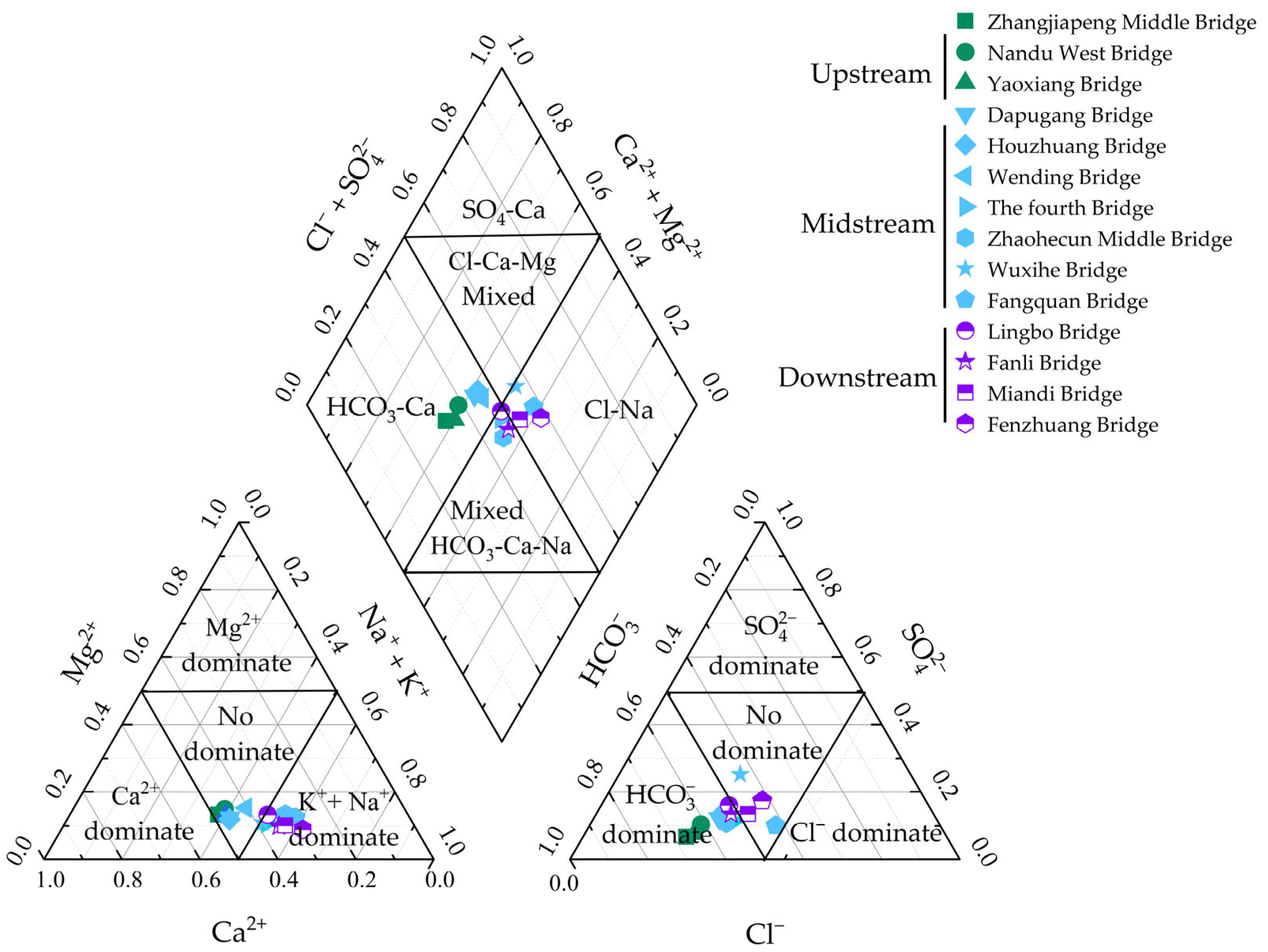
The Piper’s diagram showed that all river sampling points were distributed near the center of the diamond-shaped field (Figure 2). The upstream sampling points (Zhangjiapeng Bridge, Nanduxi Bridge, and Yaoxiang Bridge) were located to the left of the center, indicating HCO₃-Ca-type water. The downstream sampling points (Lingbo Bridge, Fanli Bridge, Fenzhuang Bridge, and Miandi Bridge) were situated to the right, representing Cl-Na-type water. The midstream sampling points fell between these two categories. In terms of the cation molar composition, ${\mathrm{Na}}^{+}+{ \mathrm{K}}^{+}$ accounted for the largest proportion (49.2%), followed by ${\mathrm{Ca}}^{2+}$ (38.6%) and ${\mathrm{Mg}}^{2+}$ (12.2%). Among anions, ${\mathrm{HCO}}_3^{-}$ was dominant (53.1%), followed by ${\mathrm{Cl}}^{-}$ (34.1%) and ${\mathrm{SO}}_4^{2-}$ (12.7%).

Following the approach of Gaillardet et al. (1999) [31], all ion ratios were calculated on a molar basis. 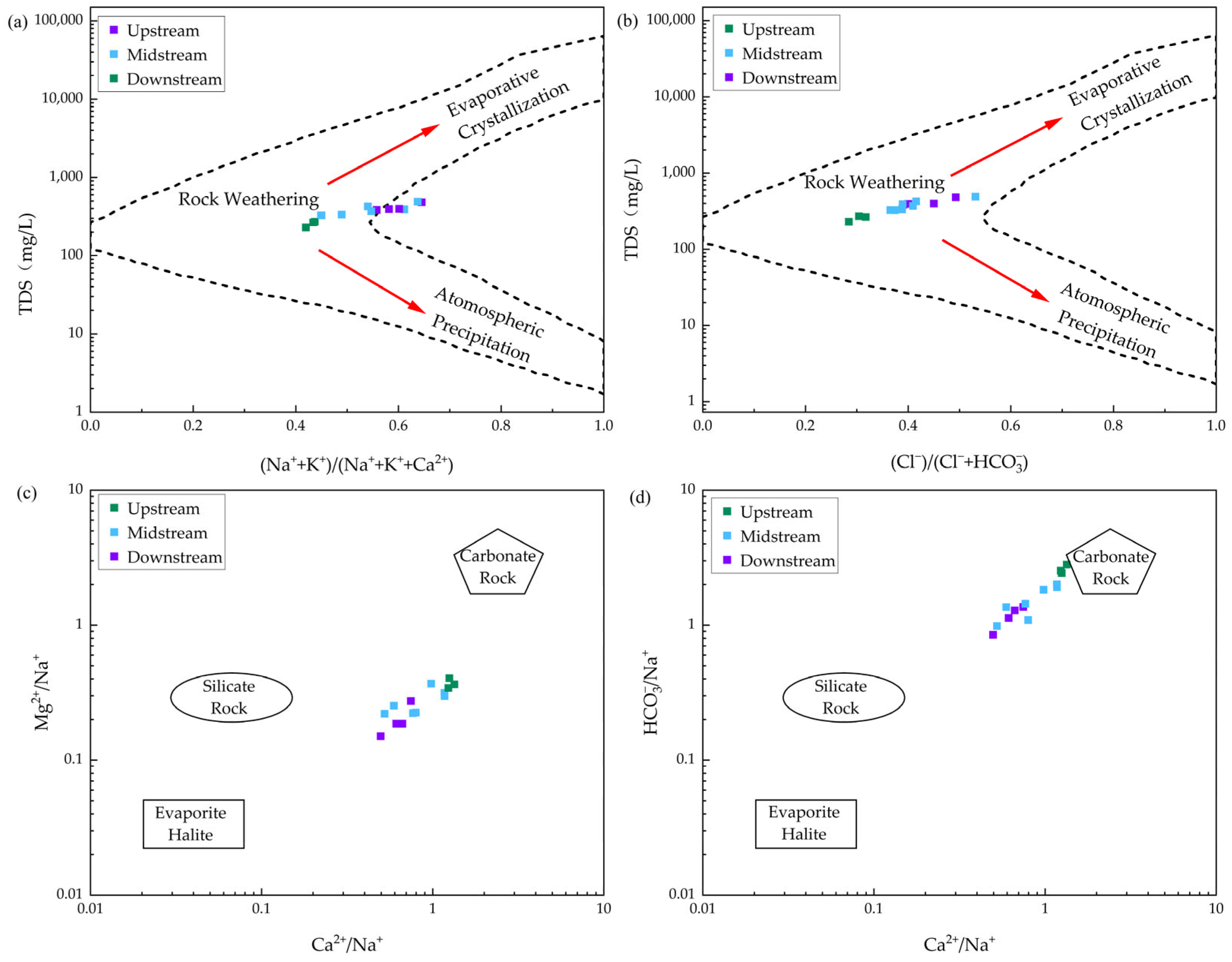Based on the relationships between ${(\mathrm{Na}}^{+}+{\mathrm{K}}^{+})/{(\mathrm{Na}}^{+}+{\mathrm{K}}^{+}+{\mathrm{Ca}}^{2+})$, ${\mathrm{Cl}}^{-}/({\mathrm{Cl}}^{-}+{\mathrm{HCO}}_3^{-})$, and TDS, the Gibbs diagram classifies the hydrochemical genesis into three categories: atmospheric precipitation, rock weathering, and evaporation–crystallization [32]. For the river samples, the values of ${(\mathrm{Na}}^{+}+{\mathrm{K}}^{+})/{(\mathrm{Na}}^{+}+{\mathrm{K}}^{+}+{\mathrm{Ca}}^{2+})$ ranged from 0.4 to 0.7, and those of ${\mathrm{Cl}}^{-}/({\mathrm{Cl}}^{-}+{\mathrm{HCO}}_3^{-})$ ranged from 0.3 to 0.6. Although the samples were mainly clustered near the rock weathering endmember, a trend toward the evaporation–crystallization endmember was observed (Figure 3). Furthermore, the ratio of ${\mathrm{Ca}}^{2+}$/${\mathrm{Na}}^{+}$ varied from 0.52 to 1.33, and that of ${\mathrm{Mg}}^{2+}$/${\mathrm{Na}}^{+}$ ranged from 0.15 to 0.37, with both falling between the carbonate and evaporite endmembers. The ${\mathrm{HCO}}_3^{-}$/${\mathrm{Na}}^{+}$ ranged from 0.85 to 2.81, lying between the carbonate, silicate, and evaporite endmembers (Figure 3).

The Huxi Catchment is predominantly composed of carbonate rocks, with only minor silicate rocks and no evaporite rocks [17]. Nevertheless, the hydrochemistry of the rivers in the middle and lower reaches shifted toward the evaporite and evaporation–crystallization endmembers (Figure 3). However, the distribution of evaporites within the study region was negligible. The observed shift toward the evaporite endmember was instead a geochemical mimicry effect caused by the input of anthropogenic salts (NaCl, CaCl₂, Na₂SO₄) from domestic wastewater and agricultural fertilizers. These anthropogenic inputs possess ionic ratios similar to those produced by evaporite dissolution, but their source is unequivocally anthropogenic, as confirmed by the spatial coincidence with urban and agricultural land use. These findings indicate that the rivers in the lower and middle reaches of Huxi Catchment are substantially influenced by anthropogenic activities.

3.3. Correlation Characteristics

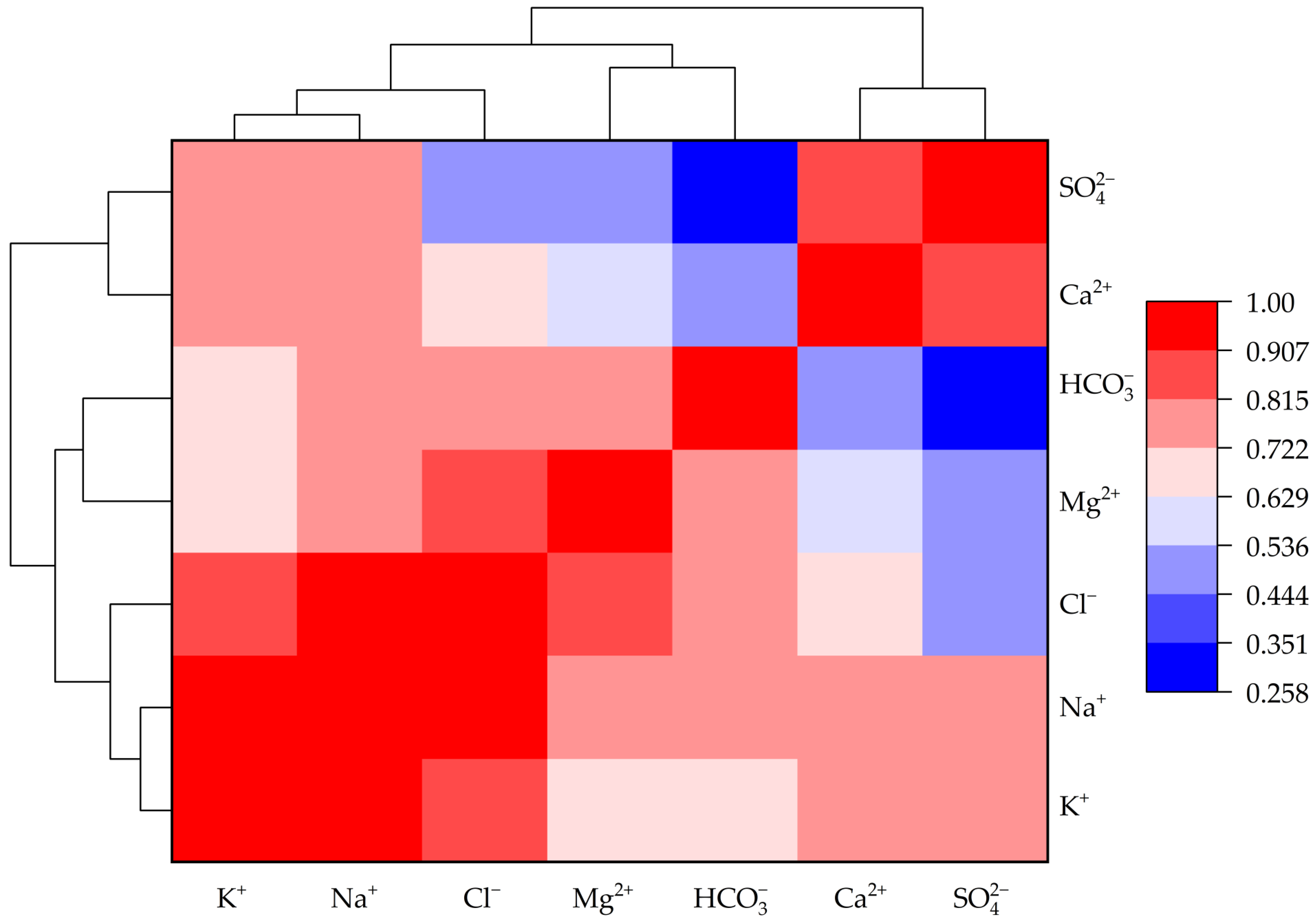
Correlation clustering analysis classified the ions into three groups: ${\mathrm{Na}}^{+}$, ${\mathrm{K}}^{+}$, and Cl⁻ formed one group; ${\mathrm{Mg}}^{2+}$ and ${\mathrm{HCO}}_3^{-}$ formed the second group; and ${\mathrm{Ca}}^{2+}$ and ${\mathrm{SO}}_4^{2-}$ formed the third group (Figure 4). This grouping likely reflects their common source characteristics. Given the absence of halite deposits in the study region, the strong association between Na⁺ and Cl⁻ is interpreted as a signature of saline anthropogenic inputs—such as domestic and industrial wastewater effluents [7]—rather than natural weathering processes. Meanwhile, the close correlation between K⁺ and Cl⁻ suggests an agricultural source, likely linked to the application of potash fertilizers. CaCO₃ and MgCO₃ are the main components of limestone, explaining the clustering of Mg²⁺ with ${\mathrm{HCO}}_3^{-}$. In contrast, ${\mathrm{Ca}}^{2+}$ was grouped with ${\mathrm{SO}}_4^{2-}$ (Figure 4). Previous studies have indicated that acid rain is a major source of ${\mathrm{SO}}_4^{2-}$ in the Taihu Lake Basin [33]. Acid rain can accelerate the weathering of carbonate rocks, thereby leading to a close correlation between ${\mathrm{SO}}_4^{2-}$ and ${\mathrm{Ca}}^{2+}$ [33]. Although the type of acid rain in the Lake Taihu Basin has shifted from sulfuric acid-dominated to nitric acid-dominated in recent years [34], the precipitation pH remains significantly correlated with the SO₂ concentrations [35]. Additionally, the close correlation between ${\mathrm{SO}}_4^{2-}$ and ${\mathrm{Ca}}^{2+}$ may also arise from shared anthropogenic sources; for example, CaSO₄ is widely used in food production as a calcium supplement carrier, curing agent, and abrasive [36].

3.4. Source Apportionment Based on PMF

To further evaluate the potential influence of anthropogenic activities, Positive Matrix Factorization (PMF) was applied. This analysis yielded the “source profiles” (

Table 2. Source profiles derived from PMF.

Characteristic	${\mathbf{K}}^{+}$	${\mathbf{Na}}^{+}$	${\mathbf{Ca}}^{2+}$	${\mathbf{Mg}}^{2+}$	${\mathbf{Cl}}^{-}$	${\mathbf{SO}}_4^{2-}$	${\mathbf{HCO}}_3^{-}$
Source 1	0.00	0.09	0.23	0.05	0.04	0.03	0.58
Source 2	0.00	0.09	0.16	0.07	0.33	0.04	0.14
Source 3	0.02	0.36	0.24	0.06	0.28	0.25	0.24
Source 4	0.02	0.55	0.14	0.07	0.46	0.04	0.50

) and “source contributions” (

Table 3. Source contributions derived from PMF.

Sample Location	Sample Name	Source 1	Source 2	Source 3	Source 4
Upstream	Zhangjiapeng Bridge	0.65	0.14	0.12	0.09
	Nanduxi Bridge	0.57	0.18	0.13	0.11
	Yaoxiang Bridge	0.51	0.22	0.22	0.05
Midstream	Dapugang Bridge	0.35	0.32	0.25	0.08
	Houzhuang Bridge	0.32	0.32	0.28	0.07
	Wending Bridge	0.31	0.18	0.15	0.36
	Sihao Bridge	0.29	0.34	0.22	0.14
	Zhaocunhe Bridge	0.25	0.29	0.17	0.28
	Wuxihe Bridge	0.19	0.10	0.56	0.15
	Fangquan Bridge	0.01	0.51	0.10	0.38
Downstream	Lingbo Bridge	0.28	0.19	0.31	0.22
	Fanli Bridge	0.28	0.16	0.21	0.35
	Miandi Bridge	0.16	0.28	0.19	0.36
	Fenzhuang Bridge	0.07	0.24	0.25	0.43

). The source profiles showed an overall balance between anions and cations (Table 2), while the source contribution rates demonstrated independence with no significant correlations (Table 3).

As shown in Table 2, Source 1 was primarily composed of Ca(HCO₃)₂, indicating a river less affected by human activities and mainly controlled by rock weathering. Source 2 consisted mainly of CaCl₂, representing a river heavily impacted by agricultural activities. This is because potassium and phosphorus from KCl and superphosphate fertilizers are readily absorbed by plants, whereas chloride and calcium ions transport into the surface water as CaCl₂. Source 3 contained NaCl, Na₂SO₄, and CaSO₄, while Source 4 was composed primarily of NaCl. Sources 3 and 4 represented rivers severely affected by wastewater discharge.

Table 3 presents the contribution of each source to the sampling sites. Source 1 contributed most to Zhangjiapeng Bridge, Nanduxi Bridge, and Yaoxiang Bridge, all of which were located upstream in the Huxi Catchment (Figure 1) and experienced minimal anthropogenic influence. Source 2 contributed the most to Fangquan Bridge, Wending Bridge, Houzhuang Bridge, and Dapugang Bridge, all of which were situated midstream (Figure 1) and were heavily affected by agricultural activities. Sources 3 and 4 collectively contributed most to Wuxihe Bridge, Fenzhuang Bridge, and Fanli Bridge, which were primarily located downstream (Figure 1) and severely affected by sewage discharge.

3.5. Source Apportionment Based on APCS-MLR

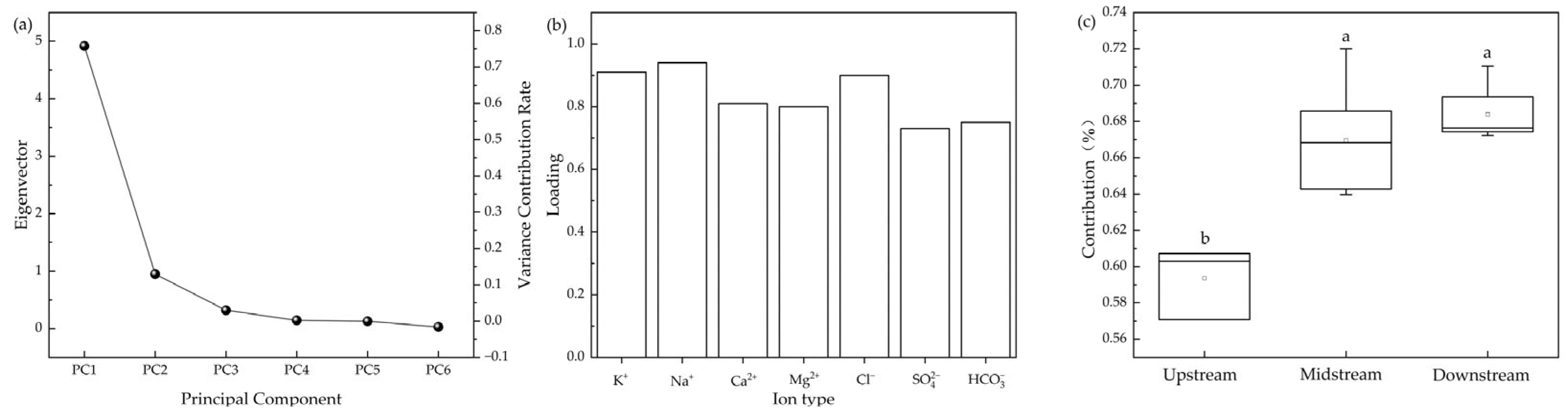
The Absolute Principal Component Score–Multiple Linear Regression (APCS-MLR) model was also employed to identify the potential sources of ions. Following Kaiser’s criterion, only the principal components with eigenvalues larger than 1 were retained [23]. The results showed that only Principal Component 1 (PC1) had an eigenvalue exceeding 1, explaining 75.6% of the total variance (Figure 5a). The factor loadings of the ions on PC1 were as follows:${\mathrm{Na}}^{+}$ (0.94) > ${\mathrm{K}}^{+}$ (0.91) > ${\mathrm{Cl}}^{-}$ (0.90) > ${\mathrm{Ca}}^{2+}$ (0.81) > ${\mathrm{Mg}}^{2+}$ (0.80) > ${\mathrm{HCO}}_3^{-}$ (0.75) > ${\mathrm{SO}}_4^{2-}$ (0.73) (Figure 5b). The loadings of ${\mathrm{Na}}^{+}$ (0.94) and ${\mathrm{Cl}}^{-}$ (0.90) were higher than those of ${\mathrm{Ca}}^{2+}$ (0.81) and ${\mathrm{HCO}}_3^{-}$ (0.75), implying that PC1 may reflect the trend of river salinization driven by anthropogenic activities. The contribution of PC1 exhibited an increasing trend from upstream to downstream; it was significantly lower upstream than in midstream and downstream. Although no significant difference was observed between midstream and downstream, the contribution remained slightly higher downstream (Figure 5c).

3.6. Source Apportionment Based on PCA-EMM

To further verify the above inference by PMF, two distinct anthropogenic endmembers were characterized using source-specific sampling strategies. Representative signatures of domestic wastewater were obtained from treated effluent collected at the outfalls of municipal wastewater treatment plants. This approach captures the integrated chemical fingerprint of the domestic sewage discharged into the river network. Representative signatures of agricultural inputs were obtained from water-soluble extracts of farmland topsoil (0–20 cm). This approach simulates the chemistry of soil pore water available for leaching and surface runoff—the primary hydrological pathway for agricultural solutes to enter the receiving water body.

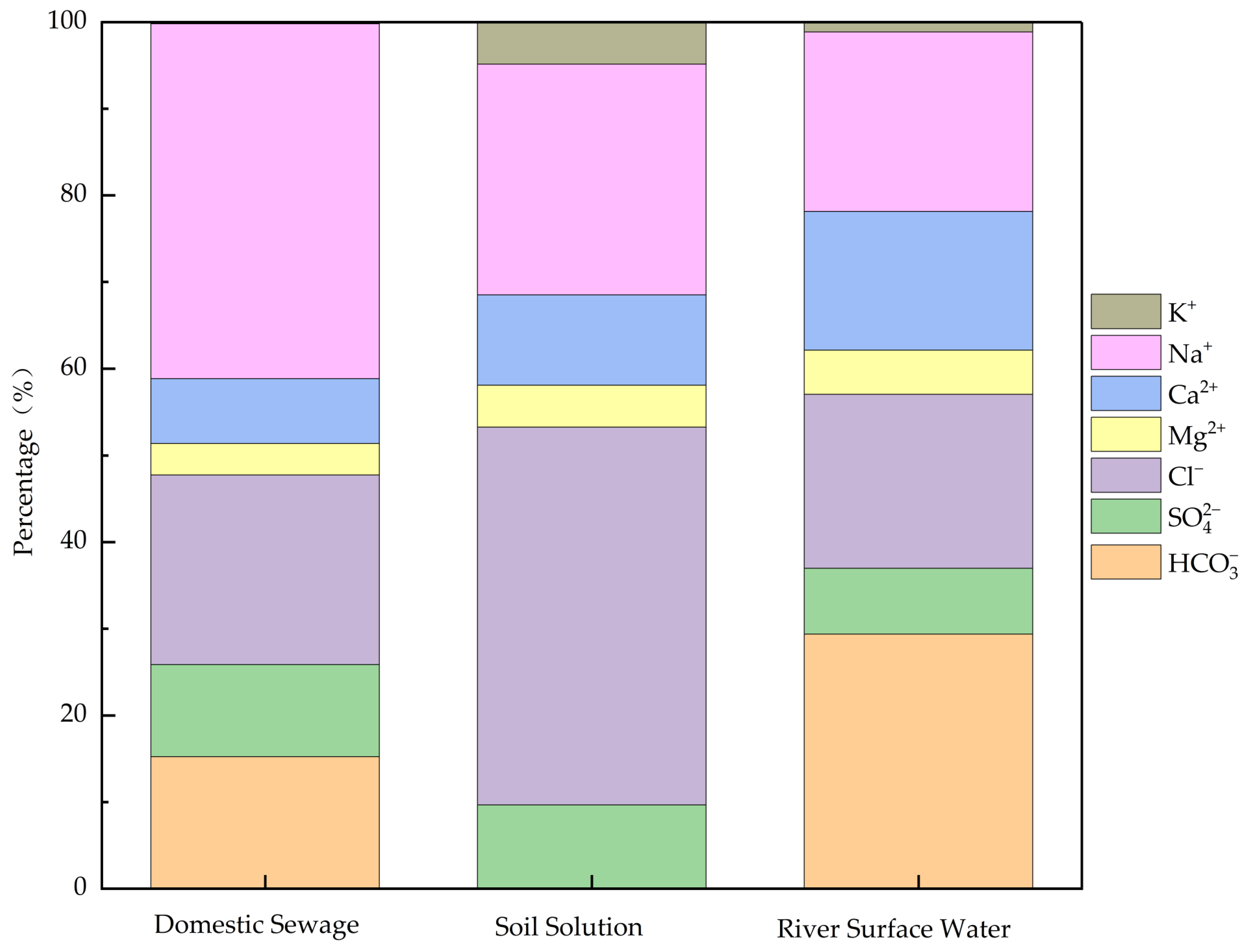
Ion concentrations in the effluent from domestic sewage treatment plants and in soil solutions from farmland were analyzed. Because the ion concentrations in these two types of samples were not directly comparable, compositional normalization was applied. The results revealed distinct ion composition characteristics among river water, domestic sewage, and soil solutions. Compared with the river water, both domestic sewage and soil solutions exhibited higher proportions of ${\mathrm{Cl}}^{-}$ and ${\mathrm{Na}}^{+}$ and a lower proportion of ${\mathrm{HCO}}_3^{-}$ (Figure 6). Moreover, ${\mathrm{Na}}^{+}$ was enriched in domestic sewage, and ${\mathrm{Cl}}^{-}$ was enriched in the soil solutions (Figure 6). It is noteworthy that the PCA-EMM method is based on relative concentrations rather than absolute values, rendering it less sensitive to dilution and evaporation effects, in contrast to absolute concentrations which exhibit substantial fluctuations in response to seasonal discharge.

Piper and Gibbs diagrams are commonly used to characterize river hydrochemistry based on specific ion molar ratios, but their ion combinations are limited. To more comprehensively elucidate the mechanisms governing river ion composition, this study applied percentage normalization to the ion molar concentrations of river water, domestic sewage, and farmland soil solutions, followed by principal component analysis (PCA) of the molar compositional data after center-log transformation. Prior to model execution, the suitability of the dataset for dimensionality reduction was evaluated statistically. The Kaiser–Meyer–Olkin (KMO) measure of sampling adequacy was 0.65, which exceeds the minimum acceptable threshold of 0.60 proposed by Kaiser (1974) [26]. 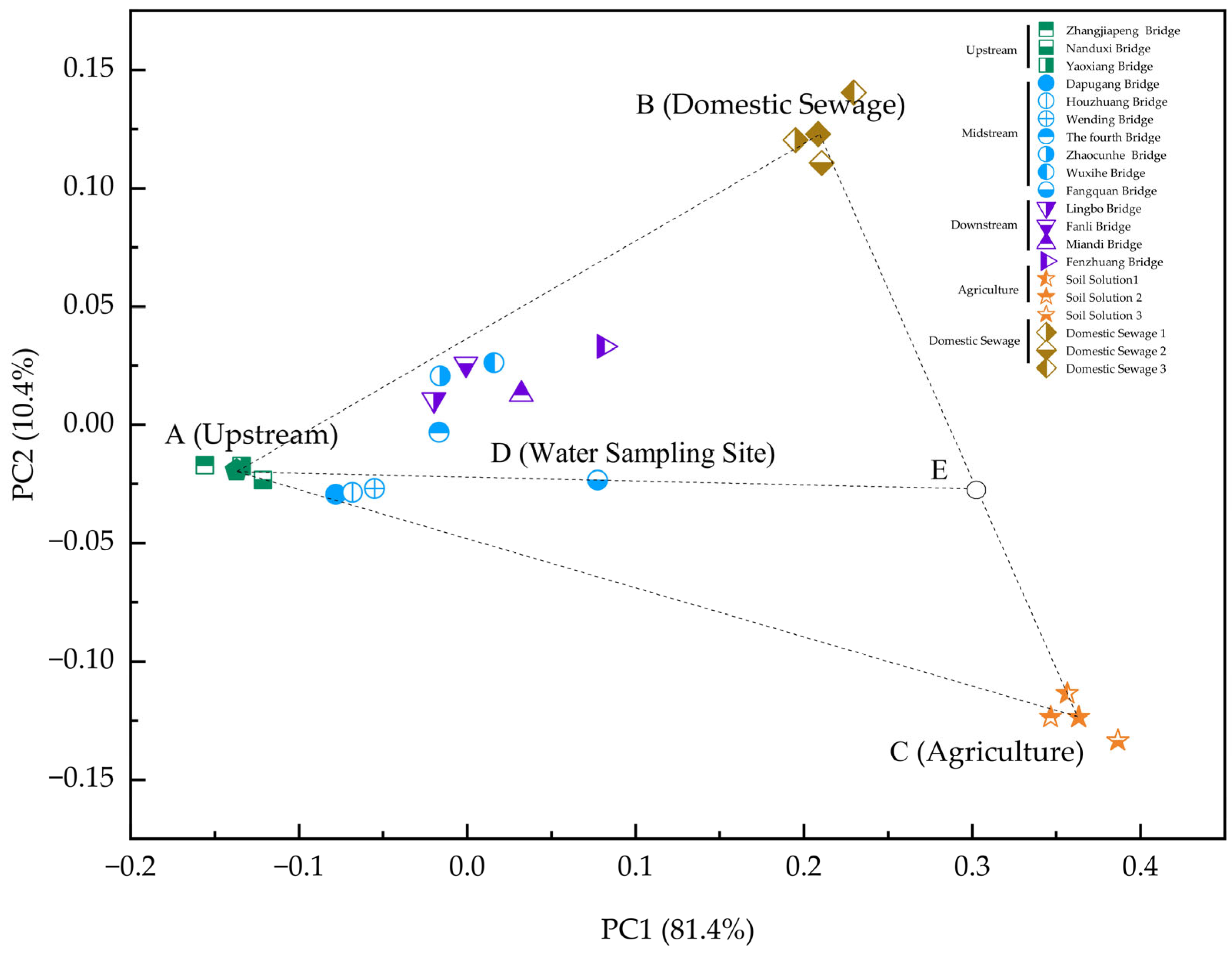Concurrently, Bartlett’s test of sphericity yielded a highly significant result (p < 0.001), confirming that the variables share sufficient common variance to justify the application of factor analysis. The first two principal components accounted for 91.8% of the total variance (PC1 = 81.4%, PC2 = 10.4%) (Figure 7), effectively distinguishing natural background from anthropogenic impacts (domestic sewage discharge and agricultural activities). PC2 was mainly driven by ${\mathrm{Cl}}^{-}$ (−0.69) and ${\mathrm{Na}}^{+}$ (0.63), serving to differentiate between domestic sewage discharge and agricultural activities (Figure 7).

Based on the principal component distribution of the sampling sites (Figure 7), the upstream water samples (Zhangjiapeng Bridge, Yaoxiang Bridge, and Nanduxi Bridge) clustered at endmember A (lower-left quadrant). Domestic sewage samples were concentrated at endmember B (upper quadrant), while farmland soil solutions were distributed at endmember C (lower-right quadrant). All river samples fell within the triangular mixing domain defined by endmembers A, B, and C. To reduce the variability associated with within-source heterogeneity, the coordinates of each endmember were defined as the mean principal component scores of the respective sample group. On this basis, an endmember mixing model was established for quantitative source apportionment. For any given sample D, vector A–D was extended to intersect line B–C at point E, and the contribution was calculated using the geometric relationships shown in Figure 7.

➀

Total contribution by anthropogenic activities = |AD|/|AE| × 100%.

➁

Contribution by agricultural activities = |AD|/|AE| × |BE|/|BC| × 100%.

➂

Contribution by domestic sewage = |AD|/|AE| × |CE|/|BC| × 100%.

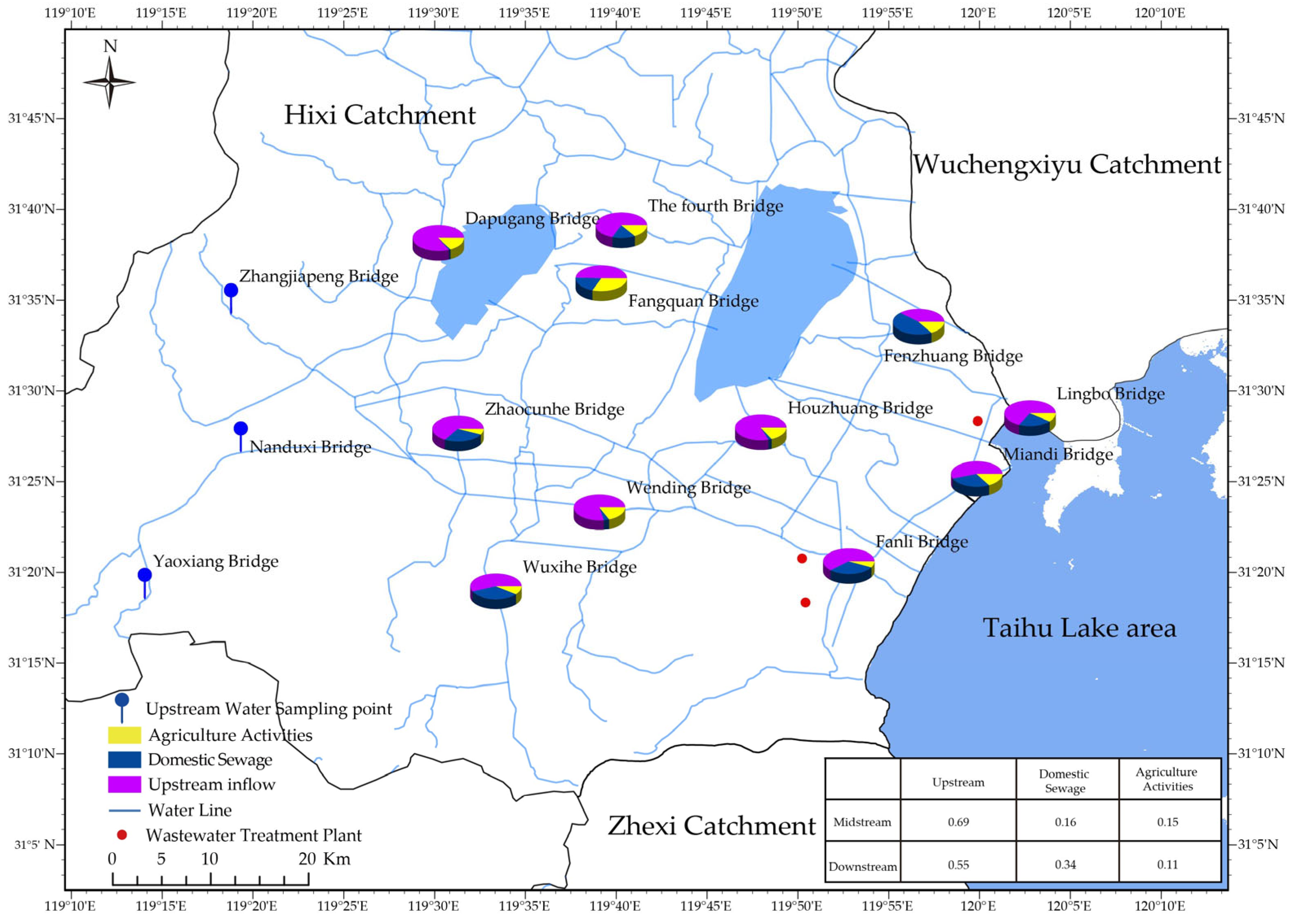
In midstream areas, upstream inflow (natural background) contributed 69%, with sewage discharge and agricultural activities accounting for 16% and 15%, respectively. In downstream areas, upstream inflow contributed 55%, while sewage discharge and agricultural activities accounted for 34% and 11%, respectively (Figure 8). These results indicate a progressively increasing influence of human activities from upstream to downstream. Notably, agricultural activities had a larger impact midstream than downstream, whereas sewage discharge exerted a stronger influence downstream than midstream (Figure 8).

In the upstream reaches, where natural background processes dominate, and the TDS concentrations remain approximately 200 mg/L, management efforts should prioritize ecological conservation. Anthropogenic inputs must be strictly controlled to maintain the low-salinity baseline. In the midstream reaches, where agricultural contributions account for approximately 15% of the total ionic load, and the TDS rises to 250–400 mg/L, salinity control should focus exclusively on agricultural non-point sources. Recommended measures include promoting balanced fertilization based on soil testing, reducing the excessive application of chloride-containing potash fertilizers (e.g., KCl), and thereby decreasing the Cl⁻ load exported from farmland drainage into the river network. In the downstream reaches, where domestic wastewater contributions reach 34%, and the TDS ranges from 300 to 400 mg/L, enhanced source control is essential. This entails restricting the discharge of high-salinity industrial effluents into municipal sewer systems and promoting the adoption of low-sodium alternatives in household and industrial products.

3.7. Comparison of PMF, APCS-MLR, and PCA-EMM Models

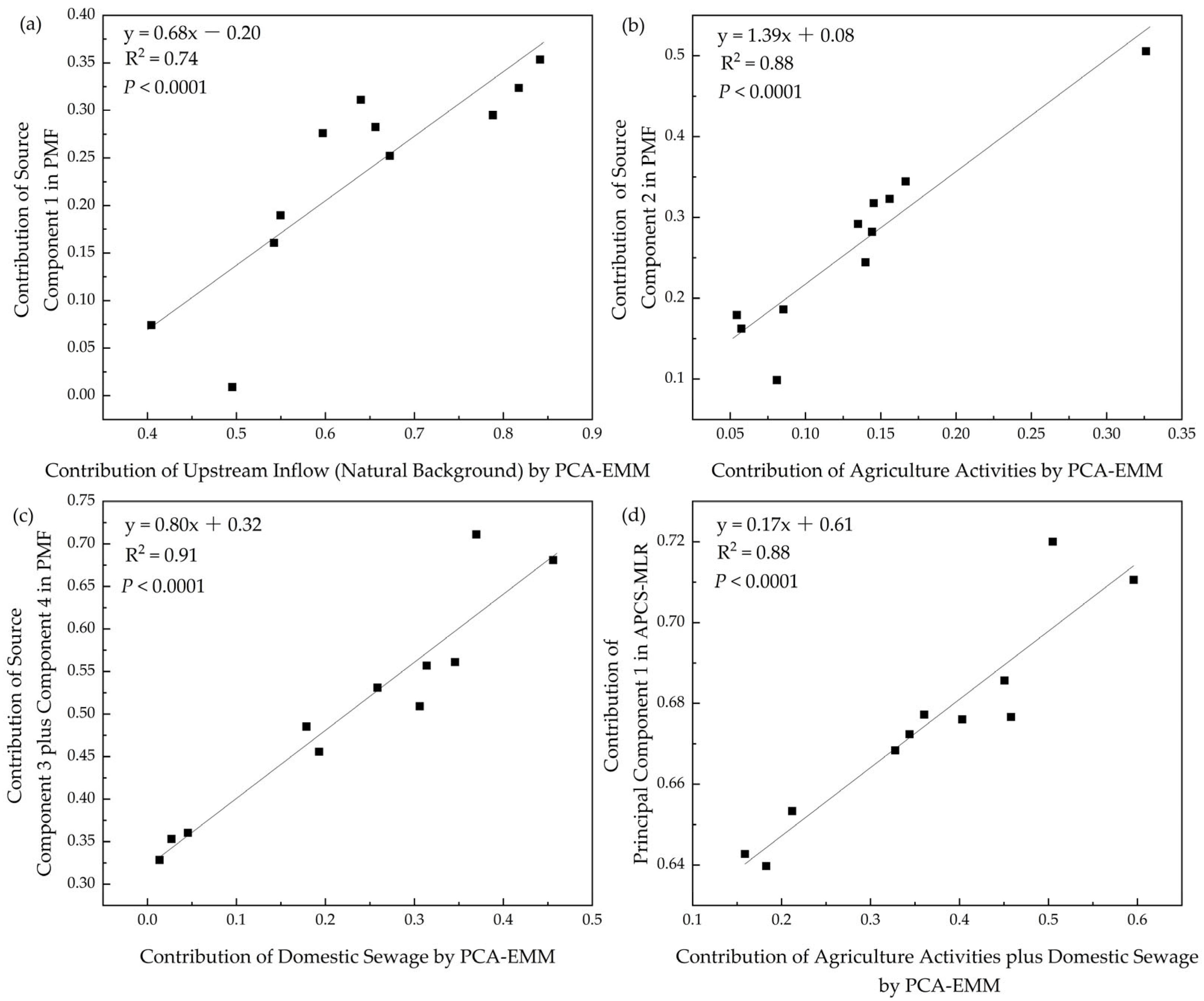
Correlation analysis between the PCA-EMM model (based on ion composition) and the PMF model (based on ion concentration) revealed strong correlations; in particular, the contribution of upstream inflow (natural background) was highly correlated with PMF source 1 (R² = 0.74, p < 0.001), agricultural activities with PMF source 2 (R² = 0.88, p < 0.001), and domestic sewage with the combined contributions of PMF source 3 and 4 (R² = 0.91, p < 0.001) (Figure 9). These results demonstrate the strong correlation between the two models, both of which effectively identify the potential impacts of agricultural activities and domestic sewage on the river hydrochemistry. PCA-EMM directly incorporated empirically measured endmember compositions (Figure 7). In contrast, PMF operates by decomposing the covariance matrix of the river water dataset into a set of statistically independent factors, which is important because agricultural runoff and domestic wastewater exhibit markedly different ionic associations. For instance, agricultural inputs are typically enriched in Cl⁻, whereas domestic wastewater carries a pronounced Na⁺ signature (Figure 6). The PMF naturally segregates these signatures into separate factors (Table 2), thereby capturing the endmember covariance patterns of each anthropogenic input. Despite this fundamental methodological difference, both models resolve the same underlying hydrochemical structure.

However, compared to PCA-EMM (15–60%), the PMF result (35–99.3%) may overestimate the contribution of anthropogenic impacts (including both sewage discharge and agricultural activities). PMF derives source profiles solely from the internal covariance structure of the river water data, constrained by non-negativity. These profiles represent extreme river compositions under heavy source influence rather than the actual hydrochemical fingerprints of the raw source inputs in PAC-EMM. Consequently, when these factor profiles are interpreted as representing pure anthropogenic inputs, the apportionment tends to amplify the anthropogenic signal and overestimate the contributions quantitatively. Given the strong correlation between the PMF and PCA-EMM results, PMF is valuable for exploratory source identification, whereas PCA-EMM provides a more conservative and hydrochemically constrained estimate of the anthropogenic contributions.

The APCS-MLR model identified only one integrated potential source, and its contribution showed a significant positive correlation with the total anthropogenic influence (including both sewage discharge and agricultural activities) derived from the PCA-EMM method (Figure 9). However, this model failed to further distinguish between the individual contributions of sewage discharge and agricultural activities because APCS-MLR is based on principal component analysis (PCA), which assumes that sources are orthogonal [23]. In actual aquatic environments, the chemical signatures of agricultural activities and sewage discharge partially overlap (Figure 6), making statistical separation via PCA challenging.

Based on the above analysis, in hydrochemistry source apportionment, PMF can first be used to preliminary identify potential sources. Field validation should then be conducted based on the PMF results to clarify the actual source characteristics. Subsequently, the PCA-EMM method can be applied to integrate hydrochemistry data from multiple sources and quantify their contributions, thereby enhancing the reliability and interpretability of source apportionment.

3.8. Research Limitations and Future Prospects

Despite the consistent source apportionment results obtained from both PMF and PCA-EMM, several limitations warrant acknowledgment and provide direction for future investigation. A principal constraint of the current modeling framework lies in its reliance on bulk ionic composition to define endmember signatures. Because certain anthropogenic sources—most notably domestic sewage, livestock effluent, and some industrial wastewaters—share broadly similar ionic fingerprints (e.g., concurrent enrichment in Na⁺, Cl⁻, and ${\mathrm{SO}}_4^{2-}$), the model possesses limited discriminatory power between sources with overlapping hydrochemical signatures. In the present study, the domestic wastewater endmember was defined using treated municipal effluent; however, contributions from unsewered livestock operations or food-processing discharges in the catchment may be partially conflated with this domestic signal. Consequently, the apportioned “domestic” fraction should be interpreted as an aggregate of household and chemically similar point-source inputs rather than a strictly residential contribution.

A further limitation of this study pertains to its temporal scope. The sampling campaign was confined to March 2025, representing dry-season, low-flow conditions when salinity reaches its annual maximum. While this design intentionally captures the period with the highest water salinity, the findings do not directly characterize the wet-season or high-discharge conditions. Although the PCA-EMM method relies on relative ion concentrations—which are inherently less sensitive to dilution and evaporation than absolute concentrations—the relative activation of different source types (e.g., surface runoff from agricultural land versus continuous point-source discharges) may vary with the season. Consequently, the source contribution fractions reported here should be interpreted as dry-season estimates, and their extrapolation to annual or wet-season loads requires caution.

The U.S. EPA PMF 5.0 User Guide recommends approximately 100 samples for robust source apportionment [20,21], yet this guideline was developed for PM2.5 aerosol datasets comprising 20–40 chemical species. In contrast, the present hydrochemical dataset includes only seven major ion variables and, thus, occupies a substantially lower-dimensional feature space. Future investigations incorporating expanded spatial and temporal sampling coverage as well as a broader suite of water quality parameters—such as nitrate (NO₃⁻), bromide (Br⁻), or trace elements—beyond the limited set of major ions will be essential to further examine the uncertainty associated with sample size. Moreover, in the current study, the PCA biplot based on hydrochemical compositional data serves more as a visual corroboration of mixing relationships among samples than as a definitive quantitative unmixing model. Accordingly, we suggest that hydrochemical compositional data can be analyzed directly within the high-dimensional compositional space, without necessitating prior dimensionality reduction. Such an approach may offer a statistically more robust alternative for small hydrochemical datasets.

4. Conclusions

Different source apportionment models (APCS-MLR, PMF, PCA-EMM) were compared in this study. The APCS-MLR model effectively captured the overall influence of anthropogenic activities but could not further differentiate between agricultural activities and domestic sewage. In contrast, the PMF model successfully distinguished the impacts of these two sources but overestimated their values. PCA-EMM integrated ionic characteristics from multiple sources, which was more reliable and interpretable than the PMF. Quantitative analysis using PCA-EMM indicated that the natural background (upstream), sewage discharge, and agricultural activities contributed 63%, 23%, and 14%, respectively. Spatially, the contribution of agricultural activities was higher midstream, whereas that of domestic sewage was higher downstream.