Geo-AI Ensemble Modeling Framework for Assessing Groundwater Contamination Under Anthropogenic Pressures in an Extensive Peri-Urban Agricultural Aquifer to Support Sustainable Groundwater Management

Abstract

Rapid urbanisation and intensified agriculture are major drivers of groundwater contamination in peri-urban agricultural aquifers worldwide. Contaminants including nitrates and phosphates accumulate through fertilizer use, wastewater infiltration, and groundwater overextraction, creating complex spatial and temporal patterns. Quantifying these impacts under multiple anthropogenic pressures remains a key challenge for effective water resource management. This study develops a Geo-AI ensemble modeling framework that integrates grid-based spatial analysis with advanced machine learning to assess groundwater contamination dynamics. A composite contamination index (CCI) was constructed to synthesize hydrochemical indicators into a unified measure of aquifer degradation. The AI framework uses Graph Neural Networks (GNNs), Light Gradient Boosting Machine (LightGBM), and Deep Long Short-Term Memory Networks (LSTM). Anthropogenic drivers include population growth, infrastructure density, agricultural intensity, groundwater abstraction, and hydroclimatic variability, providing a comprehensive understanding of contamination sources. The methodology was applied to the urbanised aquifer of Manouba, western suburban Tunis (Tunisia), using 295 samples collected from 85 monitoring wells between 2005 and 2025. Validation results show strong predictive performance, with LightGBM achieving R² = 0.986, RMSE = 13.14, and MAE = 1.72, outperforming GNNs (R² = 0.972) and LSTM (R² = 0.943). The spatial analysis reveals a major shift in contamination patterns, with severe contamination expanding to 55% of the study area in 2025, compared with 7% in 2005, while low and slight contamination declined from 45% to 20%. The results highlight how urban expansion reduces recharge, increases pollutant loading, and amplifies aquifer vulnerability, while agricultural intensification further accelerates contaminant accumulation and degradation processes. This framework provides a transferable, data-driven tool for mapping contamination hotspots and supporting targeted, sustainable groundwater management in peri-urban agricultural aquifers under increasing anthropogenic pressures worldwide.

1. Introduction

One of the greatest tasks facing our world today is to harmonize financial advancement, equitable societal participation, and the preservation of natural ecosystems in order to ensure long-term global progress [1,2,3,4]. In 2015, the Member Countries of the United Nations approved the 2030 Agenda, which identifies universal access to safe water as one of its Sustainable Development Goals [5]. Across the world, over 2.5 billion individuals rely each day on subsurface freshwater reserves, widely recognized as a reliable and uncontaminated supply for human consumption [6,7]. On a global scale, the expansion of cities and densely populated areas has severely undermined the condition and purity of underground water resources [8,9]. The expansion of urban areas often stimulates financial development and enhances overall quality of life; nevertheless, it simultaneously generates multiple contamination sources, including industrial discharges, household wastewater, and leaking sewer infrastructure [10,11], all of which pose serious risks to subsurface water systems. Although numerous investigations have documented the adverse consequences associated with urban growth [8,12,13], the measurable and statistically defined linkage between urban expansion processes and the condition of groundwater resources remains insufficiently clarified. Accordingly, clarifying this interconnection is crucial, particularly with regard to shifts in land use and land cover driven by urban growth and broader anthropogenic pressures, in order to equip policymakers with solid scientific foundations for the sustainable oversight and safeguarding of groundwater resources.

Investigations examining how variations in land utilization and surface cover patterns influence the condition of subsurface water systems, particularly under intensifying human-induced stresses, trace their origins to 1984, when pioneering work was launched by the United States Geological Survey [14]. From that point forward, researchers have applied a wide range of methodological approaches to investigate this interaction. Conventional analytical tools, including statistical correlation measures and hypothesis-based significance assessments, primarily identify associative patterns or levels of statistical relevance, yet they exhibit substantial methodological constraints [15,16,17]. In pursuit of greater analytical rigor and enhanced predictive reliability, researchers have introduced alternative quantitative frameworks, including geographically weighted regression (GWR), structural equation modelling (SEM), and random forest (RF) algorithms [18,19,20]. Despite these advancements, geographically weighted regression (GWR) and structural equation modeling (SEM) face constraints related to spatial sampling density and model specification, whereas random forest (RF) approaches are primarily confined to patterns detectable within the training dataset and may struggle with extrapolating beyond observed trends [16,18,20]. Moreover, the uneven spatial distribution of groundwater monitoring points limits the accuracy of traditional models. To overcome this, the study introduces a novel quantitative framework that applies spatial grids to maps of human-driven land changes, enhancing both the precision and efficiency of detecting variations in groundwater quality. In recent years, machine learning (ML) techniques have transformed environmental predictive modeling, offering more robust and data-driven insights under the influence of anthropogenic pressures [21,22,23]. Machine learning offers advanced tools to interpret intricate, nonlinear datasets, revealing hidden patterns and relationships that traditional statistical techniques often fail to detect [24]. Nonetheless, the use of machine learning to examine human-driven land changes at a fine spatial grid scale has received limited attention. Consequently, this study emphasizes combining a grid-based framework with ML algorithms to generate more robust and dependable insights.

A transformative phase in the safeguarding of subsurface water systems has emerged through the adoption of machine learning frameworks, with artificial intelligence technologies playing a central and pioneering role in advancing groundwater resource protection [21,22,24]. For machine learning applications, the attainment of accurate and dependable predictive performance fundamentally depends on the availability of comprehensive, well-structured, and reliable data for model training [21,22]. Accordingly, developing reliable training datasets requires a rigorous and accurate assessment of groundwater conditions. Conventional evaluation approaches generally rely either on expert-based qualitative judgments or exclusively on standardized quantitative indicators, rather than integrating both perspectives within a unified framework [16,17,18,19,20]. Approaches grounded in professional judgment draw heavily on individual expertise; however, they are intrinsically susceptible to bias because specialists often assign unequal importance to influencing variables [23,24]. Moreover, these techniques can fail to detect latent patterns and subtle relationships embedded within groundwater data records [25,26]. Methods based exclusively on computational or mathematical formulations can disregard the interpretative knowledge of specialists, which may ultimately compromise the reliability and validity of the resulting assessments [26]. To address these shortcomings, contemporary approaches increasingly combine expert-driven evaluations with quantitative analytical frameworks. Recent advances in Geo-AI ensemble modeling have enabled more robust and precise assessments of groundwater contamination under complex anthropogenic pressures. In particular, Graph Neural Networks (GNNs) capture spatial dependencies among monitoring wells [27,28,29], Light Gradient Boosting Machine (LightGBM) models identify nonlinear interactions between environmental predictors and contaminant concentrations [23,30,31], and Deep Long Short-Term Memory Networks (LSTM) account for temporal trends in groundwater quality over extended periods [32,33,34,35]. Building on these developments, this study develops a Composite Contamination Index (CCI), which integrates outputs from GNN, LightGBM, and LSTM within an optimization framework to reconcile expert-driven and data-driven weightings, thereby maximizing the combined informational value of spatial, temporal, and predictor-contaminant relationships for a comprehensive assessment of aquifer degradation.

Understanding the influence of human-driven land and resource pressures on groundwater quality is critical for safeguarding aquifer systems globally. Despite its importance, efforts to develop frameworks that capture these relationships at a fine, point-by-point spatial resolution remain scarce. To address this limitation, we propose a novel approach that integrates spatial grid sampling with advanced machine learning models, enabling a detailed and data-driven analysis of how anthropogenic pressures affect groundwater contamination patterns. The Manouba peri-urban basin, located in the western suburbs of Tunis, serves as a key agricultural and residential zone where groundwater constitutes the primary source for both domestic consumption and irrigation [36]. Between 2005 and 2025, the basin experienced rapid urban expansion and population growth, increasing from approximately 0.35 million to 0.52 million inhabitants, driven by suburban development and intensified peri-urban agriculture. This accelerated anthropogenic activity has introduced multiple contaminants into groundwater, including nitrates from fertilizers, wastewater infiltration, and emerging organic pollutants. Human-driven land changes and urban expansion in Manouba are therefore major pressures degrading aquifer quality and heightening the vulnerability of the local population.

Given these conditions, the Manouba peri-urban basin represents an ideal case study for examining the interactions between anthropogenic pressures and groundwater contamination through our Geo-AI ensemble framework. The specific objectives of this research are: (1) to characterise the spatial and temporal patterns of human-driven land changes and urbanisation in the Manouba basin; (2) to evaluate groundwater quality by integrating subjective expert judgment with objective data-driven methods; and (3) to implement a novel grid-based framework that couples machine learning models with spatial sampling to quantify the impacts of anthropogenic pressures on groundwater contamination. The findings offer a data-driven, transferable framework to support sustainable groundwater management under increasing anthropogenic pressures in peri-urban agricultural aquifers.

2. Study Area and Data Collection

2.1. Study Area

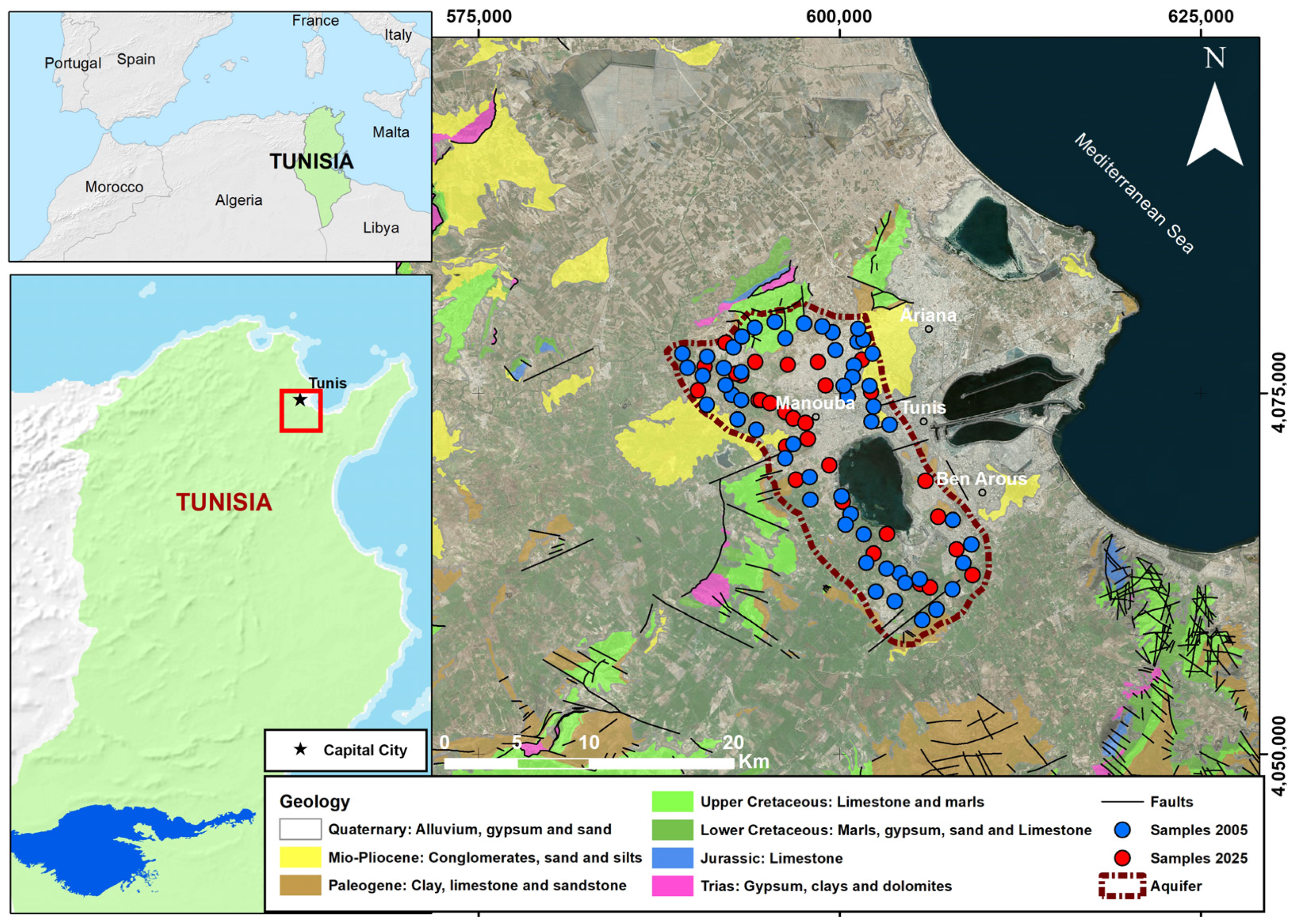
The study area is the Manouba peri-urban basin, situated in the western suburban fringe of Tunis, northern Tunisia (Figure 1). The basin extends over approximately 160 km², with elevations generally ranging between 10 and 120 m above sea level. It represents a strategic peri-urban agricultural zone where rapid residential expansion and intensive farming coexist [37,38]. The basin is bordered by the Tebourba plain to the west and the urban agglomeration of Tunis to the east, forming a transitional interface between metropolitan development and irrigated agricultural lands. The terrain is relatively flat to gently undulating, facilitating both urban sprawl and agricultural intensification [39].

The Medjerda River, the principal fluvial system in northern Tunisia, flows in proximity to the basin and plays a significant role in regional hydrological dynamics [36,39]. The area is characterized by a Mediterranean semi-arid climate, marked by mild, wet winters and hot, dry summers [36,40]. The mean annual temperature is approximately 18 °C, with summer maxima frequently exceeding 40 °C [36]. Average annual precipitation ranges between 400 and 450 mm, occurring predominantly from October to March, while potential evapotranspiration surpasses rainfall during most of the year, contributing to water stress conditions [36,39,40].

Geologically, the Manouba basin is composed mainly of Quaternary alluvial deposits overlaying Mio-Pliocene formations [36,40,41,42]. The shallow aquifer system consists primarily of unconsolidated sands, silts, gravels, and clayey intercalations with variable thickness, typically between 20 and 80 m. Hydrogeologically, the aquifer is predominantly phreatic and highly vulnerable to surface-derived contamination due to its shallow water table and permeable sedimentary structure [36,41,42,43]. Recharge occurs mainly through rainfall infiltration, irrigation return flows, and lateral contributions from surrounding highlands, while groundwater extraction for domestic supply and agricultural irrigation constitutes the dominant discharge mechanism. Regional hydraulic gradients generally direct groundwater flow toward the northeast, following the topographic slope and converging toward lower-lying zones influenced by urban development and agricultural activity [41,43].

2.2. Data Collection and Processing

Groundwater monitoring in the Manouba peri-urban basin was conducted through two sampling campaigns representing distinct stages of anthropogenic pressure. In total, 295 samples were collected from 85 shallow phreatic wells: 223 samples obtained from 54 monitoring wells in 2005 and 72 samples from 31 wells in 2025. All samples were drawn from the unconfined aquifer system, which is particularly vulnerable to surface-derived contamination due to its limited depth and permeable alluvial deposits. The geographic coordinates of each sampling location were recorded to enable precise spatial analysis. Prior to sampling, wells were purged to ensure representative groundwater conditions, after which samples were collected, preserved under controlled temperature conditions, and transported for laboratory analysis within an appropriate timeframe to maintain data integrity.

It is acknowledged that the groundwater samples collected in 2005 and 2025 were obtained from partially different sets of monitoring wells. As a result, the temporal comparison does not rely on paired observations from identical locations. To address this limitation, both datasets were analyzed within a consistent geospatial framework. Hydrochemical parameters from each period were interpolated and aggregated onto a common spatial grid, allowing for a harmonized comparison of groundwater quality patterns across the study area.

This approach reduces the influence of individual well variability and enables the assessment of regional-scale temporal changes in groundwater quality. While the absence of identical sampling points may introduce some uncertainty in local-scale comparisons, the relatively large number of samples in each period supports a robust characterization of spatial trends and their evolution over time.

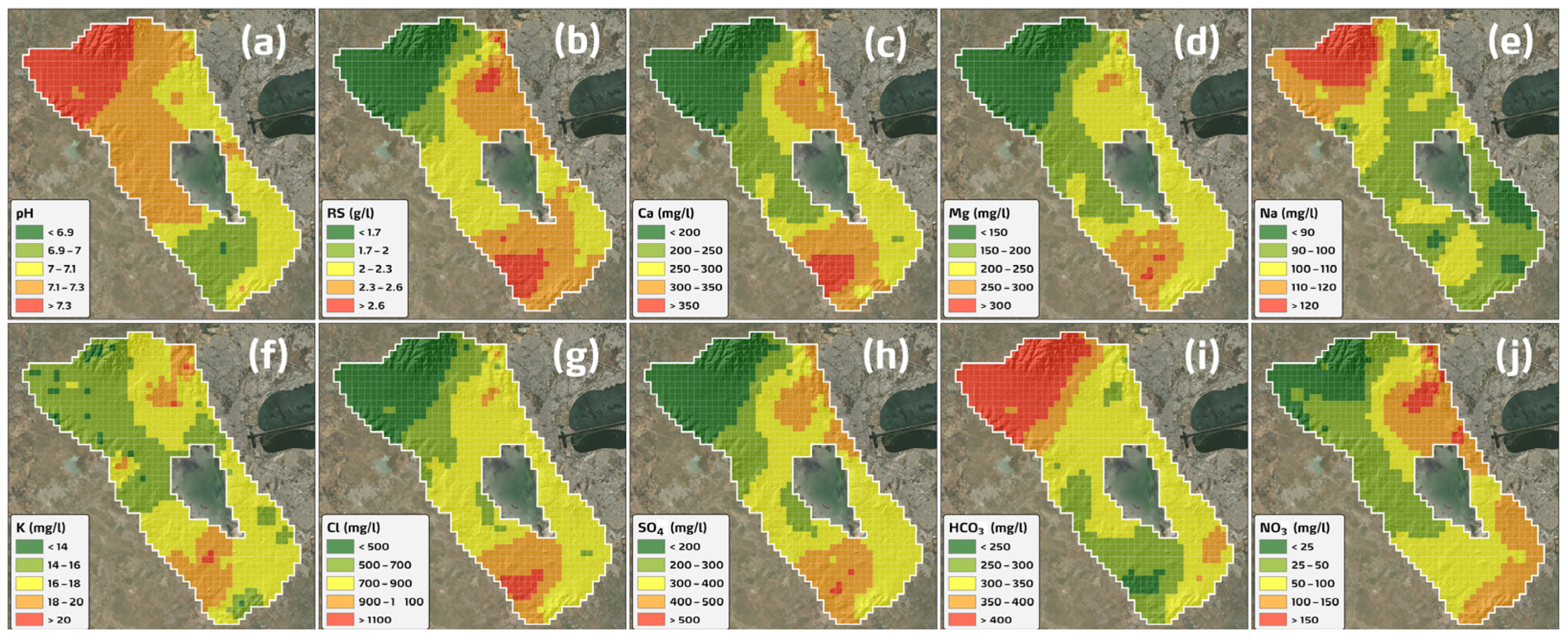
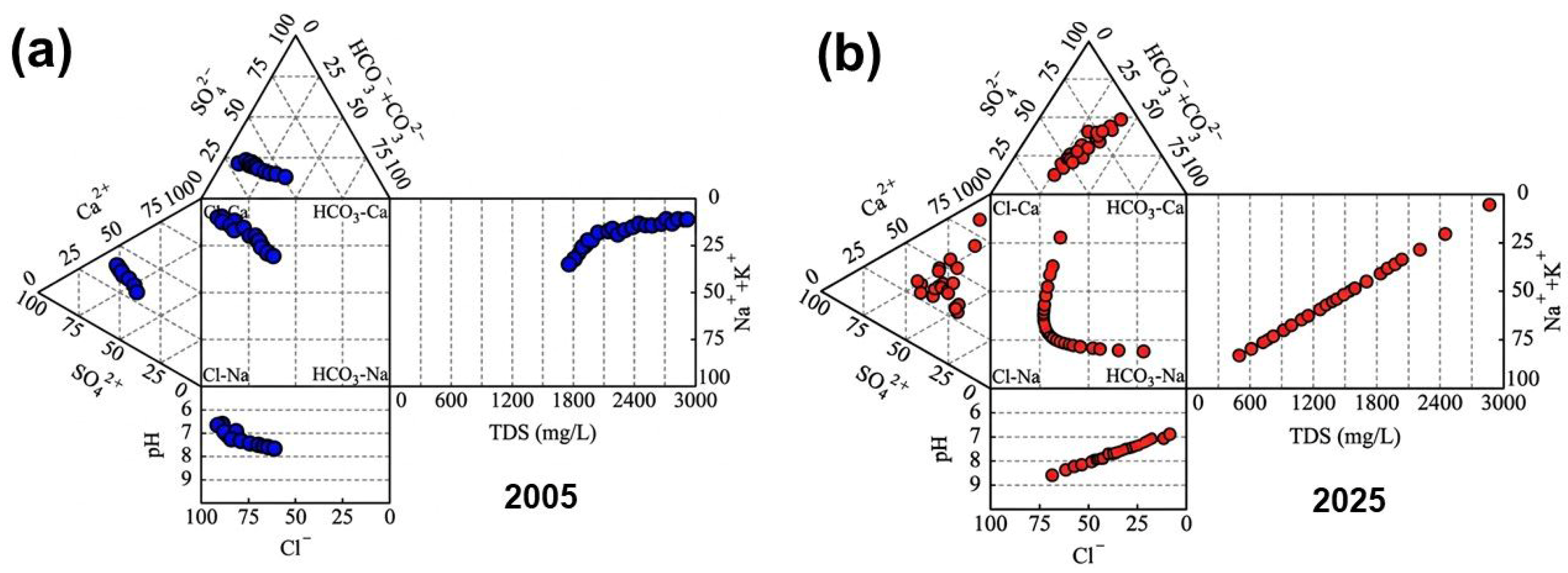
The hydrochemical assessment included major physicochemical indicators and ionic constituents, namely pH, total dissolved solids (TDS), potassium (K⁺), sodium (Na⁺), calcium (Ca²⁺), magnesium (Mg²⁺), chloride (Cl⁻), bicarbonate (HCO₃⁻), sulfate (SO₄²⁻), and nitrate (NO₃⁻). Field measurements were conducted for in situ parameters, while laboratory analyses were performed using standardized analytical procedures to quantify major cations and anions. Data reliability was ensured through systematic quality control protocols, including duplicate sampling, blank controls, and verification of analytical precision. The ionic charge balance error was calculated for each sample, and only results within an acceptable uncertainty threshold (±5%) were retained for further analysis.

In addition to hydrochemical data obtained from groundwater sampling campaigns, ancillary datasets were incorporated to account for potential anthropogenic drivers influencing groundwater quality. These include land use/land cover maps derived from remote sensing data (e.g., urban areas, cultivated lands, and natural covers), which were used as proxy indicators of human pressure on the aquifer system. These spatial datasets enable the characterization of surface activities that may contribute to groundwater contamination through recharge modification, pollutant infiltration, and surface runoff processes.

Although direct measurements of groundwater abstraction volumes and discharge rates were not available at the scale of the study, land-use indicators, particularly the extent of urbanized and agricultural areas, were used as indirect proxies for anthropogenic pressure. These proxies are commonly adopted in hydrogeological studies when direct pumping or discharge records are limited or unavailable.

The groundwater datasets collected in 2005 and 2025 are treated as two independent temporal snapshots representing distinct hydrochemical conditions of the aquifer system. The optimization procedures applied in this study are not based on the assumption of temporal stationarity of groundwater contamination. Instead, they are used to derive weights and indices that are applicable within each dataset and to enable spatial comparison between the two time periods. Consequently, the approach does not assume that contamination levels remain constant over time, but rather quantifies their evolution by comparing two independent observations of the system at different dates.

3. Composite Contamination Index (CCI)

Reliable quantification of groundwater contamination under intensifying anthropogenic pressures requires a weighting strategy that reconciles hydrogeochemical variability with expert-driven environmental interpretation. Weighting schemes derived solely from professional judgment may introduce epistemic uncertainty due to differences in expert perception of contaminant relevance, whereas purely statistical approaches can overlook hydrogeological processes and contextual aquifer vulnerability [44,45,46]. In peri-urban agricultural systems such as the Manouba basin, where contamination arises from interacting urban expansion, agricultural intensification, and groundwater abstraction, an integrated weighting framework is therefore essential to produce a robust and interpretable contamination metric. To address this challenge, we developed a Composite Contamination Index (CCI) based on a hybrid methodology that combines structured subjective prioritization through the Best-Worst Method (BWM) with objective data-driven weighting using the CRITIC approach [47,48,49,50,51]. Final weights are determined via constrained quadratic optimization, ensuring mathematical consistency while preserving both conceptual and statistical information.

3.1. Indicator Standardization

Ten hydrochemical indicators were considered: pH, total dissolved solids (TDSs), potassium (K⁺), sodium (Na⁺), calcium (Ca²⁺), magnesium (Mg²⁺), chloride (Cl⁻), bicarbonate (HCO₃⁻), sulfate (SO₄²⁻), and nitrate (NO₃⁻). Because these variables differ in scale, unit, and environmental significance, direct aggregation would distort their relative contribution. Therefore, normalization was required to transform all indicators into dimensionless contamination intensities.

For contamination-type parameters whose impact increases proportionally with concentration, normalization was performed as (Equation (1)):

$$z_{ij}={\displaystyle \frac{x_{ij}}{S_j}}$$

(1)

where x_ij represents the value of the j-th parameter for the i-th sample, s_j denotes the standard deviation of the j-th parameter across all samples, and z_ij is the standardized value (z-score) of the j-th parameter for the i-th sample. For pH, whose environmental risk depends on deviation from an acceptable standard value, the following formulation was used (Equation (2)):

$$z_{ij}={\displaystyle \frac{\left|x_{ij}-S_j\right|}{S_j}}$$

(2)

In this formulation, x_ij represents the value of indicator j for sample i, while S_j denotes the reference value (e.g., the mean or standard deviation depending on the adopted normalization scheme) of indicator j across all samples. The term z_ij is the normalized value of indicator j for sample i, computed as a relative deviation from the reference value S_j. This transformation allows the indicators to be expressed on a comparable scale by accounting for their relative variability and magnitude. The resulting normalized matrix is subsequently used in the aggregation and weighting procedures of the contamination assessment framework.

3.2. Subjective Weighting Using the Best–Worst Method

The Best–Worst Method (BWM) was applied to derive structured subjective weights based on hydrogeological expertise regarding contamination drivers in the peri-urban aquifer. The preference judgments were established by the author based on a synthesis of published studies and prior experience in similar hydrogeological settings. Experts first identified the most influential indicator (Best) and the least influential indicator (Worst) in terms of groundwater degradation. Pairwise preference ratios were then assigned to express the relative importance between the Best indicator and each of the remaining indicators, as well as between all indicators and the Worst one.

The optimization problem is formulated as (Equation (3)):

minξ

(3)

subject to (Equation (4))

$$\left\{\begin{array}{c}\left|{\displaystyle \frac{w_B}{w_j}}-a_{Bj}\right|\le \xi \\ \left|{\displaystyle \frac{w_j}{w_W}}-a_{jW}\right|\le \xi \\ \sum _{j=1}^n{w}_j=1,w_j\ge 0\end{array}\right.$$

(4)

In this formulation, w_j represents the subjective weight assigned to indicator j. The terms w_B and w_W correspond to the weights of the Best and Worst indicators, respectively. The coefficient a_Bj denotes the preference intensity of the Best indicator over indicator j, while a_jW expresses the preference of indicator j over the Worst indicator. The scalar ξ represents the maximum deviation to be minimized, ensuring consistency in pairwise comparisons. The solution of this constrained optimization yields the subjective weight vector that best satisfies the expert preference structure while maintaining normalization.

3.3. Objective Weighting Using the CRITIC Method

To complement the expert-based approach, the CRITIC method was implemented to quantify the intrinsic informational contribution of each indicator. This method evaluates both the variability of each variable and its redundancy relative to others.

The informational content of indicator j is computed as (Equation (5)):

$$C_j={\sigma }_j{\sum }_{k=1}^n\left(1-r_{jk}\right)$$

(5)

and the corresponding objective weight is obtained through normalization (Equation (6)):

$$w_j^{CRITIC}={\displaystyle \frac{C_j}{{\sum }_{j=1}^n{C}_j}}$$

(6)

Here, σ_j denotes the standard deviation of the normalized values of indicator j, reflecting its contrast intensity across the study area. The coefficient r_jk represents the Pearson correlation coefficient between indicators j and k, quantifying redundancy. The term C_j therefore captures the combined effect of dispersion and independence. Indicators exhibiting high variability and low correlation with others receive greater objective weight because they provide more unique information about contamination processes.

3.4. Weight Optimization and Classification of CCI

To reconcile subjective and objective weighting schemes, an integrated weight vector was obtained by minimizing the total squared deviation between the final weights and both preliminary weight sets (Equation (7)):

$$min{\sum }_{j=1}^n\left[{\left(w_j-w_j^{BWM}\right)}^2+{\left(w_j-w_j^{CRITIC}\right)}^2\right]$$

(7)

subject to (Equation (8)):

$${\sum }_{j=1}^n{w}_j=1,w_j\ge 0$$

(8)

In this equation, wjw_jwj represents the optimized integrated weight for indicator j, while w_j^BWM and w_j^CRITIC denote the subjective and objective weights, respectively. The quadratic minimization ensures that the final weights remain statistically stable while preserving expert knowledge. This dual-consistency mechanism enhances methodological robustness and reduces weighting bias.

The Composite Contamination Index for groundwater sample i is calculated as (Equation (9)):

$${CCI}_i={\sum }_{j=1}^n{w}_j{z}_{ij}$$

(9)

where CCI_i represents the aggregated contamination intensity at location i, obtained by summing the product of the optimized weight w_j and the standardized contamination score z_ij across all indicators. This weighted aggregation captures both exceedance magnitude and relative importance.

To facilitate interpretation for groundwater management, the CCI values were classified into five contamination categories as shown in

Table 1. Classification of Composite Contamination Index (CCI).

Rank	Contamination Level	CCI Range
1	Low contamination	CCI ≤ 0.5
2	Slight contamination	0.5 < CCI ≤ 1.0
3	Moderate contamination	1.0 < CCI ≤ 1.5
4	High contamination	1.5 < CCI ≤ 2.0
5	Severe contamination	CCI > 2.0

.

These thresholds reflect increasing exceedance intensity relative to regulatory standards and were calibrated based on the statistical distribution of contamination scores within the peri-urban aquifer system.

4. Geo-AI Grid-Based Modeling

4.1. Methodological Framework

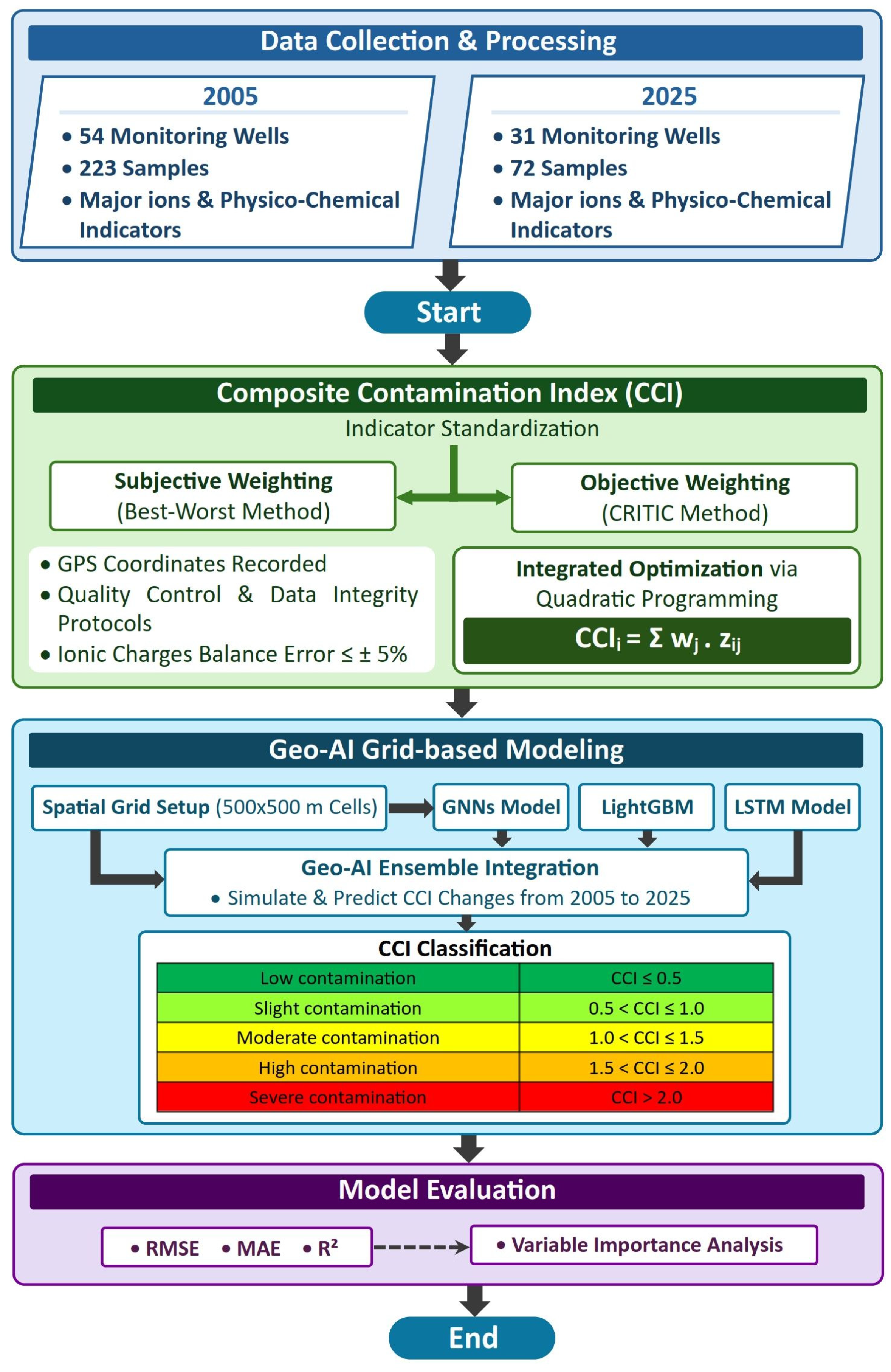
To quantify land transformations and related anthropogenic pressures in the Manouba peri-urban aquifer from 2005 to 2025, a spatially explicit grid-based framework was applied (Figure 2). Rather than relying on administrative boundaries, the study employed a regular lattice in which each cell represented an independent spatial-temporal unit. Land-change datasets for 2005 and 2025 were overlaid onto this grid to enable consistent assessment of surface transitions and pressure dynamics over the twenty-year period.

It is important to note that the groundwater sampling campaigns conducted in 2005 and 2025 do not consist of identical monitoring wells. Therefore, temporal changes in groundwater quality are not evaluated at the level of individual wells, but rather at the spatial distribution level across the study area.

To address this, hydrochemical data from both periods were integrated within a geospatial framework, and spatial interpolation combined with grid-based aggregation was used to ensure comparability between the two time slices. This approach allows the characterization of overall temporal trends in groundwater quality by comparing spatial patterns of contamination indicators (e.g., CCI) between 2005 and 2025, rather than relying on paired time-series observations at fixed monitoring points.

Each grid cell measures 500 m × 500 m (0.25 km²), ensuring a suitable compromise between spatial resolution and computational efficiency. At the raster scale, each cell contains 18 × 18 pixels, allowing aggregation of pixel-level land information into standardized analytical units while reducing local noise. The grid was generated using ArcGIS 10.8 to ensure geometric consistency and accurate alignment of multi-temporal data. After removing cells lacking valid land-change information, 900 effective grid units were retained to support the analysis of spatiotemporal anthropogenic pressure intensification.

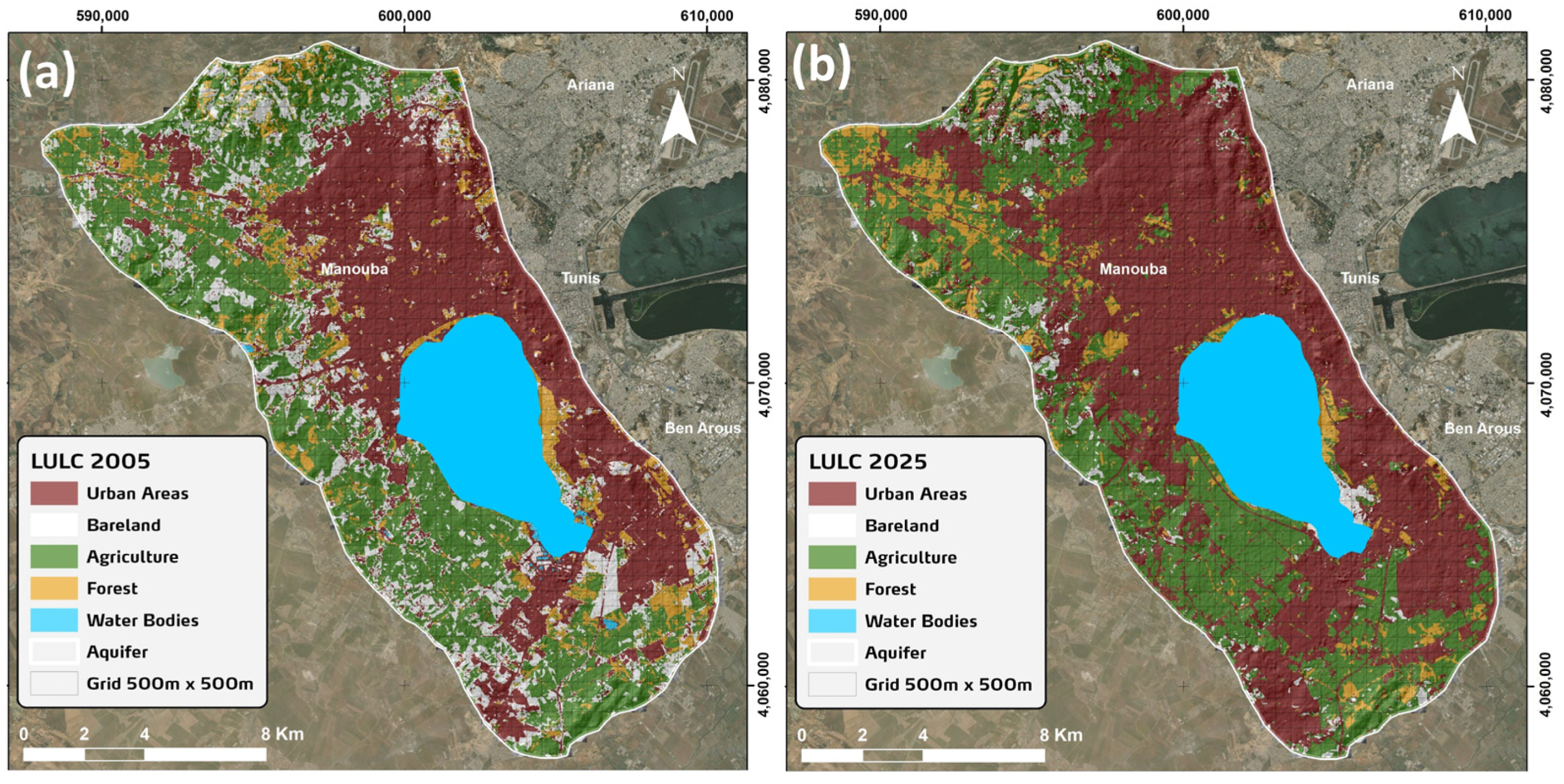
A centroid sampling point was assigned to each grid cell to ensure consistent data extraction. For every unit, the proportional extent of key land categories linked to anthropogenic pressures (urban areas, bare land, agriculture, forest, and water bodies) was calculated for 2005 and 2025 (Figure 3). The LULC maps were generated through remote sensing data processing using Landsat 7 ETM+ imagery for 2005 and Landsat 8 OLI imagery for 2025. Temporal change was quantified by computing percentage differences between the two years, reflecting both the magnitude and direction of land-use transformation.

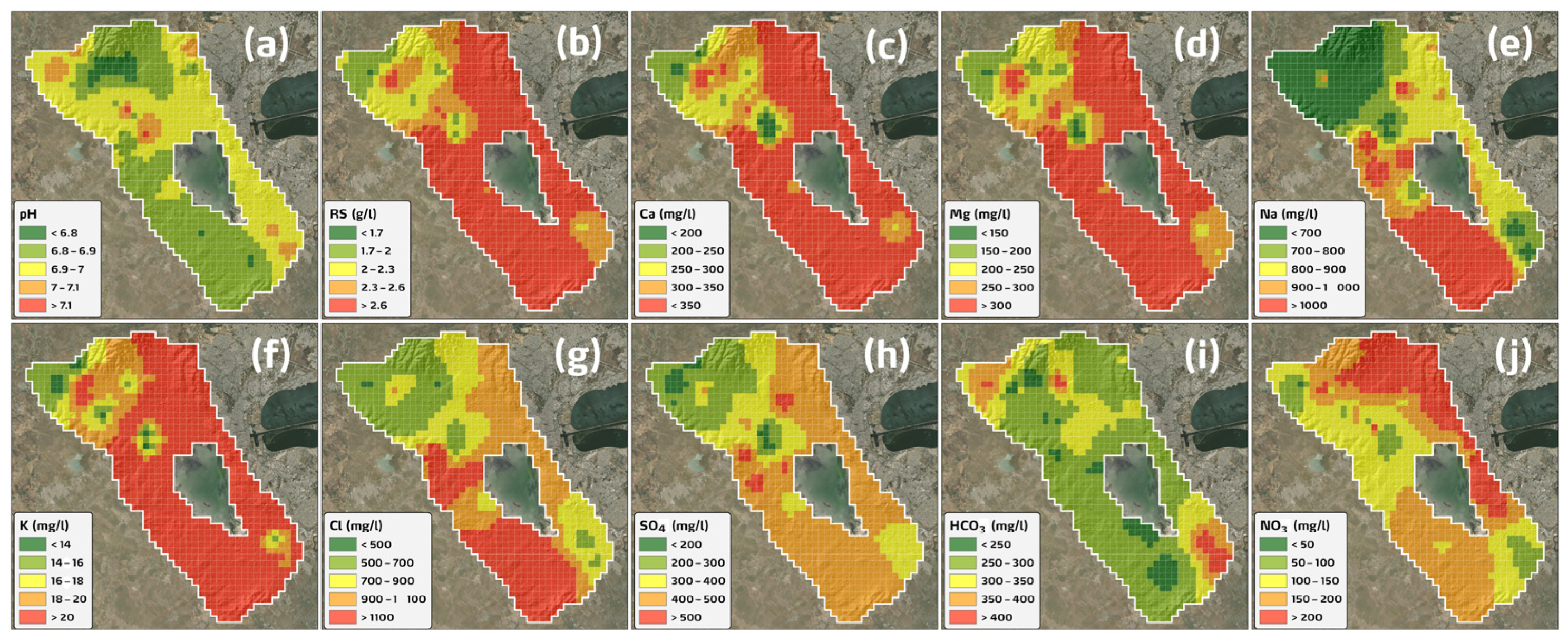
To link land dynamics with groundwater conditions, hydrochemical parameters and Composite Contamination Index (CCI) values for 2005 and 2025 were averaged within each grid cell. The evolution of groundwater contamination was then expressed as a relative change rate derived from CCI values (Equation (10)).

$$E={\displaystyle \frac{{CCI}_{2025}-{CCI}_{2005}}{{CCI}_{2005}}}$$

(10)

In this formulation, E represents the proportional variation in contamination intensity over the 2005–2025 interval, while CCI₂₀₀₅ and CCI₂₀₂₅ represent the Composite Contamination Index values at the initial and final years, respectively. This normalized indicator allows comparison of contamination progression irrespective of baseline conditions.

The calculated land-transformation proportions and aggregated hydrochemical variables were subsequently used as predictor features in machine learning models to simulate and predict the spatial evolution of CCI over the study period. For clearer interpretation and mapping, the predicted CCI change rates for 2025 were converted back into absolute CCI values, allowing direct comparison with observed contamination patterns. The overall methodological framework is summarized in Figure 2.

4.2. Geo-AI Model Selection and Architecture

The expansion of groundwater monitoring in the Manouba peri-urban aquifer has produced high-dimensional datasets with spatial heterogeneity, temporal variability, and nonlinear interactions driven by land changes and anthropogenic pressures. Traditional statistical methods struggle to capture these complexities, whereas advanced Geo-AI approaches can model nonlinear relationships, learn hierarchical features, and integrate spatial structure for more accurate predictions.

To develop the Geo-AI Ensemble Modeling Framework for Assessing Groundwater Contamination under Anthropogenic Pressures, three complementary algorithms were employed: Graph Neural Networks (GNNs) for spatial connectivity, Light Gradient Boosting Machine (LightGBM) for efficient nonlinear feature modeling, and Deep Long Short-Term Memory Networks (LSTM) for temporal dynamics. Collectively, these models capture the spatial, structural, and temporal dimensions of contamination under evolving land transformations.

4.2.1. Graph Neural Networks (GNNs)

Groundwater contamination patterns exhibit strong spatial dependency due to hydraulic connectivity and shared anthropogenic drivers [27,28,29]. To explicitly incorporate spatial structure, the study area was represented as a graph G = (V,E), where grid cells correspond to nodes V, and edges E represent spatial adjacency or hydrogeological connectivity.

The graph convolution operation is expressed as (Equation (11)):

$$H^{(l+1)}=\sigma \left({\mathrm{Ñ}}^{-1/2}{\mathrm{Ã}\mathrm{Ñ}}^{-1/2}{H}^{\left(l\right)}{W}^{\left(l\right)}\right)$$

(11)

where à = A + I denotes the adjacency matrix with self-loops, Ñ is the corresponding degree matrix, H^(l) represents node features at layer l, W^(l) is the trainable weight matrix, and σ is a nonlinear activation function. The initial feature matrix H⁽⁰⁾ includes land-change proportions, anthropogenic pressure indicators, and hydrochemical variables.

The final node representation is mapped to predicted CCI change rates through (Equation (12)):

$${\widehat{y}}_i=f\left(H_i^{\left(L\right)}\right)$$

(12)

where H_i^(L) denotes the learned embedding of node i after L graph convolution layers, and ŷ_i represents the predicted contamination change rate. By propagating information across neighboring cells, GNNs effectively capture spatial diffusion effects and localized anthropogenic influences.

4.2.2. Light Gradient Boosting Machine (LightGBM)

To model complex nonlinear relationships between land transformations and groundwater contamination, LightGBM was employed as a high-performance gradient boosting framework [23,30,31]. LightGBM constructs an ensemble of decision trees in a sequential manner, minimizing a differentiable loss function.

At iteration t, the objective function is defined as (Equation (13)):

$${\mathcal{L}}^{\left(t\right)}={\sum }_{i=1}^{n}l\left(y_i,{\widehat{y}}_i^{(t-1)}+f_t\left(x_i\right)\right)+\mathsf{\Omega }\left(f_t\right)$$

(13)

where y_i is the observed CCI change rate, ŷ_i^(t−1) is the previous prediction, f_t represents the newly added decision tree, and Ω(f_t) is a regularization term controlling model complexity.

The prediction at iteration ttt is updated as (Equation (14)):

$${\widehat{y}}_i^{\left(t\right)}={\widehat{y}}_i^{(t-1)}+{\eta f}_t\left(x_i\right)$$

(14)

where η denotes the learning rate. By iteratively correcting residual errors, LightGBM efficiently captures nonlinear interactions among land-change proportions, anthropogenic indicators, and hydrochemical variables while reducing overfitting through regularization.

4.2.3. Deep Long Short-Term Memory Networks (LSTM)

Groundwater contamination evolution reflects cumulative and delayed effects of anthropogenic pressures [32,33,34,35]. To model temporal dependencies across the 2005–2025 interval, a deep LSTM architecture was implemented. LSTM networks incorporate gated memory mechanisms that regulate information flow across time steps.

The forget, input, and output gates are formulated as (Equation (15)):

$$\left\{\begin{array}{c}{f}_t=\sigma \left(W_f{x}_t+U_f{h}_{t-1}+b_f\right)\\ i_t=\sigma \left(W_i{x}_t+U_i{h}_{t-1}+b_i\right)\\ o_t=\sigma \left(W_o{x}_t+U_o{h}_{t-1}+b_o\right)\end{array}\right.$$

(15)

where x_t represents the input feature vector at time t, h_t−1 is the previous hidden state, and W, U, and b denote trainable parameters. The gates control memory updating and state propagation, enabling the network to learn long-term contamination trends driven by progressive land transformations.

The final output layer produces predicted CCI change rates based on the learned temporal representation. By capturing delayed hydrochemical responses to anthropogenic pressures, LSTM enhances temporal forecasting capability.

4.2.4. Ensemble Integration

To leverage complementary strengths, outputs from GNN, LightGBM, and LSTM models were integrated within an ensemble framework. Spatial dependencies captured by GNN, nonlinear feature interactions modeled by LightGBM, and temporal evolution learned by LSTM collectively improve predictive robustness. This integrated Geo-AI architecture strengthens the assessment of groundwater contamination under land changes and anthropogenic pressures, directly supporting sustainable groundwater management in the extensive peri-urban agricultural aquifer.

4.3. Data Preparation and Normalization

For the Geo-AI ensemble framework, the input features consisted of land-change proportions, anthropogenic pressure indicators, and hydrochemical parameters from 2005 and 2025, while the output was defined as the change rate of the Composite Contamination Index (CCI) over the 2005–2025 period. Prior to model training, all input variables were normalized to eliminate differences in units and scales among hydrochemical and land-change parameters, producing dimensionless values suitable for machine learning.

To mitigate overfitting and enhance model generalization, L2 regularization was applied during preprocessing. The regularized loss function is expressed as (Equation (16)):

$$L_{reg}=L\left(w\right)+\alpha {\sum }_{j=1}^n{w}_j^2$$

(16)

where L(w) is the original loss, w_j are the model weights, n is the number of input features, and α ∈ [0, 1] is the regularization coefficient controlling the strength of penalization. All preprocessing steps and normalization procedures were implemented using Python, ensuring consistency across the GNN, LightGBM, and LSTM models.

4.4. Model Performance Evaluation

Model performance was assessed using three standard metrics: the root mean squared error (RMSE), mean absolute error (MAE), and the coefficient of determination (R²), calculated as follows (Equations (17)–(19)):

$$RMSE=\sqrt{{\displaystyle \frac{1}{m}}{\sum }_{i=1}^m{\left({\widehat{y}}_i-y_i\right)}^2}$$

(17)

$$MAE={\displaystyle \frac{1}{m}}{\sum }_{i=1}^m\left|{\widehat{y}}_i-y_i\right|$$

(18)

$$R^2=1-{\displaystyle \frac{\sum _{i=1}^m{\left(y_i-{\widehat{y}}_i\right)}^2}{\sum _{i=1}^m{\left(y_i-\overline{y}\right)}^2}}$$

(19)

where y_i and ŷ_i are the observed and predicted CCI change rates for grid cell i, ȳ is the mean of observed CCI change rates, and m is the total number of samples. High predictive accuracy is indicated by low RMSE and MAE values and an R² value approaching 1.

To ensure reliable model evaluation and mitigate overfitting, the dataset was divided into training and testing subsets using a hold-out validation strategy. Model performance was assessed on unseen data, and the process was repeated using multiple random partitions to improve robustness and reduce the influence of sampling variability. The reported performance metrics correspond to the average results obtained across these repetitions. This approach is appropriate for the available dataset, which consists of a moderate number of samples with spatial heterogeneity. In addition, inherent regularization mechanisms in LightGBM and early stopping criteria (where applicable) were used to further control model complexity and enhance generalization.

To evaluate the influence of land transformations and anthropogenic pressures on groundwater contamination predictions, a variable importance analysis was conducted using permutation-based techniques [23,34,35]. This analysis highlights the relative contribution of each predictor to the modeled CCI dynamics, providing insight into which pressures most strongly drive contamination patterns in the Manouba peri-urban aquifer.

All data preprocessing, model training, and evaluation were implemented in Python (V 3.12.0) using the scikit-learn library for LightGBM and permutation analyses, PyTorch (V 2.6.0) for LSTM, and PyG (PyTorch Geometric) (V 2.6.0) for GNNs, ensuring reproducibility and computational efficiency.

5. Results

5.1. Land Changes and Anthropogenic Pressures

Understanding how land transformations and anthropogenic pressures affect groundwater quality is critical for the sustainable management of the Manouba peri-urban aquifer. To this end, spatial and temporal changes in land-use patterns between 2005 and 2025 were analyzed using land use/land cover (LULC) maps (Figure 3). In 2005 (Figure 3a), the basin was mainly characterized by urban areas and agricultural land. Urban areas covered 84.9 km² (34.1%), followed by agriculture with 75.1 km² (30.1%). Bare land represented 41.4 km² (16.6%), while water bodies accounted for 25.7 km² (10.3%), largely corresponding to the Sebkha system. Forested areas occupied 22.3 km² (8.9%). This distribution indicates a landscape where agricultural activities and urban settlements were already dominant, particularly around the central and eastern parts of the basin.

By 2025 (Figure 3b), the LULC composition had significantly changed. Urban areas expanded to 121.7 km² (48.8%), becoming the most dominant land cover class in the basin. Agricultural land remained relatively stable, slightly increasing to 76.1 km² (30.5%). In contrast, bare land decreased drastically to 9.8 km² (3.9%), suggesting that large portions of previously unused land were converted mainly into urban or agricultural uses. Forested areas declined moderately to 16.7 km² (6.7%), while water bodies remained almost stable at 25.1 km² (10.1%), reflecting the relatively constant extent of the Sebkha and associated wetlands.

The comparative analysis between 2005 and 2025 reveals that the most significant change occurred in urban areas, which increased by 36.8 km² (from 34.1% to 48.8%) over the twenty-year period. This expansion occurred largely at the expense of bare land and forest areas, which decreased by 31.6 km² and 5.6 km², respectively. Agricultural land remained relatively stable with only a minor increase of 1.0 km², indicating that farming activities continue to play an important role in the basin’s land use structure despite the rapid urban expansion.

This pronounced growth of built-up areas reflects the accelerated urbanization of the Manouba peri-urban region, driven by population growth and the spatial expansion of the Greater Tunis metropolitan area. Such land transformations intensify anthropogenic pressures on the aquifer system by increasing impervious surfaces, modifying recharge processes, and enhancing the potential for groundwater contamination through urban runoff, wastewater discharge, and intensified human activities. Therefore, understanding these LULC dynamics is essential for assessing their potential impact on groundwater quality and for developing sustainable land and water management strategies in the Manouba aquifer system.

5.2. Impact on Groundwater Chemistry

5.2.1. Hydrochemical Dynamics

To evaluate the influence of land transformation and anthropogenic pressures on groundwater quality in the Manouba peri-urban aquifer between 2005 and 2025, the principal hydrochemical parameters were statistically analysed and summarized (

Table 2. Summary of hydrochemical parameters in the Manouba peri-urban aquifer.

Parameter	2005 (223 Samples)				2025 (72 Samples)
	Min	Max	Mean	Std. Dev.	Min	Max	Mean	Std. Dev.
pH	6.88	7.40	7.17	0.15	6.69	7.19	6.91	0.13
RS (g/L)	1.41	2.90	2.08	0.46	1.61	3.92	2.52	0.71
Ca2+ (mg/L)	124.2	408.8	243.24	79.18	100.20	625.22	351.16	146.45
Mg2+ (mg/L)	97.3	318.5	186.75	62.16	85.07	506.76	289.51	125.36
Na+ (mg/L)	78.2	142.5	105.05	15.67	411.50	1277.73	748.84	255.72
K+ (mg/L)	13.7	21.5	16.40	2.24	11.70	35.10	20.35	7.07
Cl− (mg/L)	351.0	1244.3	683.05	234.04	443.70	1492.00	785.39	319.91
SO42− (mg/L)	124.9	538.0	300.97	122.39	94.62	603.26	349.16	152.63
HCO3− (mg/L)	231.9	476.0	351.63	69.66	183.05	488.13	309.79	83.82
NO3− (mg/L)	15.0	175.0	73.19	53.31	42.50	288.00	153.87	79.59

). The descriptive statistics highlight substantial temporal variations in groundwater chemistry and reveal a progressive intensification of mineralisation processes over the two-decade period.

Groundwater pH values indicate relatively stable neutral conditions throughout the study period. In 2005, pH ranged from 6.88 to 7.40 with an average value of 7.17, whereas in 2025 the range slightly shifted toward lower values (6.69–7.19) with a mean of 6.91. Although this change reflects a minor decrease in alkalinity, the overall pH distribution remains within the neutral range, suggesting that acid-base equilibrium conditions in the aquifer have remained relatively stable despite evolving anthropogenic pressures (Figure 4).

In contrast, mineralisation indicators reveal a clear increase over time. Residual salinity (RS) values ranged from 1.41 to 2.90 g/L in 2005 with an average of 2.08 g/L, whereas in 2025 they increased to a broader interval of 1.61–3.92 g/L and a higher mean value of 2.52 g/L (Table 2). This rise in RS (Residual Salinity) reflects an overall enrichment of dissolved ions in groundwater and indicates progressive salinisation of the aquifer system. The higher standard deviation recorded in 2025 (0.71 compared with 0.46 in 2005) also suggests increased spatial heterogeneity in groundwater mineralisation.

The concentrations of major cations show marked increases between the two sampling periods. Calcium concentrations rose from a mean of 243.24 mg/L in 2005 to 351.16 mg/L in 2025, while magnesium increased from 186.75 mg/L to 289.51 mg/L. Sodium exhibited the most pronounced change, with mean concentrations rising dramatically from 105.05 mg/L in 2005 to 748.84 mg/L in 2025 and maximum values reaching 1277.73 mg/L. Potassium concentrations also increased moderately, from an average of 16.40 mg/L to 20.35 mg/L. These trends indicate a significant enrichment in alkali and alkaline-earth metals, reflecting intensified geochemical interactions within the aquifer as well as growing anthropogenic influences.

Similar patterns are observed for the major anions. Chloride concentrations increased from a mean of 683.05 mg/L in 2005 to 785.39 mg/L in 2025, with maximum values rising from 1244.3 mg/L to 1492.0 mg/L. Sulfate concentrations also increased, with average values rising from 300.97 mg/L to 349.16 mg/L. In contrast, bicarbonate concentrations exhibited a slight decline, decreasing from a mean of 351.63 mg/L in 2005 to 309.79 mg/L in 2025, suggesting partial modification of carbonate equilibrium processes within the aquifer. The relative dominance of major ions indicates that Ca²⁺, Mg²⁺, and Na⁺ constitute the principal cations controlling groundwater chemistry, whereas Cl⁻, SO₄²⁻, and HCO₃⁻ represent the main anionic components.

Among the analysed parameters, nitrate shows the most alarming temporal evolution. In 2005, nitrate concentrations ranged from 15.0 to 175.0 mg/L with a mean value of 73.19 mg/L. By 2025, this range increased substantially to 42.50–288.00 mg/L with an average concentration of 153.87 mg/L, more than doubling the earlier mean value (Table 2). The large standard deviation recorded in both periods further reflects considerable spatial variability, indicating that nitrate contamination is unevenly distributed across the aquifer and strongly influenced by localized anthropogenic activities.

The comparison between the 2005 and 2025 datasets reveals a clear deterioration of groundwater quality in the Manouba peri-urban aquifer (

Table 3. Proportion of groundwater samples above WHO (2017) limits in the Manouba peri-urban aquifer: Exceedance Rate (%).

Parameter	WHO Limit	2005 Exceedance Rate (%)	2025 Exceedance Rate (%)
pH	6.5–8.5	0	0
RS (g/L)	1.0	100	100
Ca2+ (mg/L)	N/A	N/A	N/A
Mg2+ (mg/L)	N/A	N/A	N/A
Na+ (mg/L)	200	0	100
K+ (mg/L)	N/A	N/A	N/A
Cl− (mg/L)	250	100	100
SO42− (mg/L)	250	67	71
HCO3− (mg/L)	N/A	N/A	N/A
NO3− (mg/L)	50	50	94

Note: N/A: Exceedance rates are not reported for parameters without WHO guideline values.

). In both periods, total dissolved solids and chloride concentrations systematically exceeded WHO guideline values, indicating persistent salinization of the aquifer. However, a marked change occurred for sodium and nitrate. While no sodium exceedance was observed in 2005, all samples collected in 2025 surpassed the WHO guideline value, suggesting a strong intensification of salinization processes, likely related to irrigation return flows, urban wastewater infiltration, and possible seawater or saline water mixing. Nitrate contamination also increased significantly, with the exceedance rate rising from about 50% in 2005 to nearly 94% in 2025, highlighting the growing impact of agricultural fertilization and urban pollution. Sulfate exceedance remained high but relatively stable (67–71%), reflecting the combined influence of evaporite dissolution and anthropogenic inputs. These results indicate a progressive degradation of groundwater quality over the last two decades, driven by both natural hydrogeochemical processes and increasing anthropogenic pressure in the peri-urban environment.

5.2.2. Hydrochemical Spatial Patterns

Understanding the spatial configuration of groundwater chemistry is essential for interpreting contamination processes in the Manouba peri-urban aquifer under progressive land transformation and anthropogenic pressure. To generate continuous distribution surfaces of hydrochemical parameters for 2005 and 2025, a semivariogram-calibrated kriging interpolation framework was implemented in ArcGIS 10.8. This geostatistical estimator, based on spatial autocorrelation theory, provides best linear unbiased predictions by explicitly modeling the spatial dependence structure of measured concentrations.

The spatial distribution maps of hydrochemical parameters for 2005 (Figure 5) indicate that groundwater quality in the peri-urban aquifer of Manouba was mainly controlled by natural hydrogeochemical processes related to recharge conditions and water-rock interaction. The pH values range between 6.88 and 7.40, reflecting slightly alkaline to neutral conditions typical of carbonate aquifers. Higher pH values are generally observed in the northwestern sector, which corresponds to recharge zones, while slightly lower values appear toward the southern and southeastern parts of the aquifer (Figure 5a). The residual salinity (RS) varies between about 1.41 and 2.90 g/L (Figure 5b) and shows a progressive increase from the northwestern areas toward the central and southeastern sectors, following the general groundwater flow direction. This spatial gradient suggests increasing mineralization along the flow path as a result of prolonged water-rock interaction.

The distribution of major cations and anions supports this hydrogeochemical evolution. Calcium and magnesium concentrations (Figure 5c,d) are relatively low in the northwestern recharge zones and increase toward the southern and southeastern parts of the aquifer, reflecting the dissolution of carbonate and dolomitic minerals within the aquifer formations. Sodium and potassium (Figure 5e,f) display moderate concentrations with limited spatial variability, although slightly higher values appear in the central sectors, which may indicate early stages of ion-exchange processes and minor anthropogenic inputs. Chloride and sulfate concentrations (Figure 5g,h) show a clear spatial gradient, with higher values occurring mainly in the southern and southeastern sectors where concentrations locally exceed 1200 mg/L for Cl⁻ and 500 mg/L for SO₄²⁻. These patterns suggest progressive mineral enrichment along the groundwater flow path and possible contributions from evaporitic mineral dissolution. In contrast, bicarbonate concentrations (Figure 5i) are relatively higher in the northwestern and central areas, reflecting active carbonate dissolution in recharge zones. Nitrate distribution (Figure 5j) already shows localized anomalies in the central and northeastern sectors, where concentrations exceed 150 mg/L, indicating the influence of agricultural activities and peri-urban settlements.

By 2025, the spatial configuration of hydrochemical parameters (Figure 6) reveals a clear intensification of groundwater mineralization and contamination across the aquifer. The pH values slightly decrease, ranging between 6.69 and 7.19 (Figure 6a), which may reflect enhanced infiltration of anthropogenic recharge and nitrification processes in urbanized areas. Residual salinity increases significantly, reaching values close to 3.9 g/L (Figure 6b), with pronounced hotspots located in the central and eastern sectors of the aquifer. This marked increase indicates stronger evapoconcentration processes and intensified groundwater-rock interaction under conditions of increased groundwater abstraction and reduced natural recharge.

Major ion concentrations also show a substantial increase compared with 2005. Calcium and magnesium (Figure 6c,d) reach values exceeding 600 mg/L and 480 mg/L, respectively, particularly in the central and southeastern sectors, suggesting intensified carbonate and dolomite dissolution. Sodium concentrations increase dramatically (Figure 6e), locally exceeding 1200 mg/L, which may result from combined effects of evaporite dissolution, cation-exchange reactions, and anthropogenic inputs related to urban wastewater and irrigation return flows. Potassium remains relatively low but shows localized increases in the central and eastern zones (Figure 6f), likely associated with agricultural fertilization and domestic effluents.

Chloride and sulfate distributions (Figure 6g,h) indicate a significant expansion of high-salinity zones compared with 2005. Chloride concentrations exceed 1400 mg/L in several central and northeastern peri-urban areas, while sulfate values locally surpass 600 mg/L, reflecting the combined influence of evaporite dissolution and anthropogenic inputs. Bicarbonate concentrations (Figure 6i) remain moderate but show localized increases in southern sectors, indicating continued carbonate weathering during groundwater circulation. Finally, nitrate concentrations increase markedly (Figure 6j), reaching nearly 300 mg/L in several wells, with pronounced hotspots in the central and northeastern peri-urban zones. The spatial coincidence between nitrate, chloride, and sodium anomalies suggests that wastewater infiltration, septic system leakage, and urban runoff have become major contamination pathways.

The spatial evolution of hydrochemical parameters between 2005 and 2025 demonstrates a clear hydrochemical evolution of the Manouba aquifer. While groundwater chemistry in 2005 was largely controlled by natural processes such as carbonate dissolution and progressive mineralization along the groundwater flow path, the 2025 configuration reflects the growing influence of anthropogenic pressures. Rapid peri-urban expansion, intensified agriculture, industrial development, and increased groundwater abstraction appear to have significantly altered groundwater quality, leading to higher salinity levels and the emergence of localized contamination hotspots within the aquifer system.

5.3. CCI Dynamics (2005–2025)

5.3.1. CCI Spatiotemporal Patterns

Groundwater quality dynamics associated with land transformation and increasing human pressures were quantified using the Composite Contamination Index (CCI). To ensure methodological robustness, parameter weighting combined a decision-based approach and an information-driven technique. Specifically, subjective priorities were derived through the Best-Worst Method (BWM), while objective contrasts among variables were obtained using the CRITIC method. The final weight coefficients resulted from integrating both schemes, providing a balanced representation of expert judgment and statistical variability.

The CCI values were subsequently computed using the aggregated weights and classified into five contamination categories ranging from low contamination to severe contamination.

In 2005, groundwater quality conditions were relatively balanced across the study area. Low contamination covered approximately 25% of the area, while 20% showed slight contamination. Moderate contamination represented the largest share (30%), followed by 18% classified as high contamination and 7% as severe contamination (Figure 7a). Spatially, the western and north-western sectors were dominated by low and slight contamination classes, indicating relatively preserved groundwater conditions. In contrast, moderate to high contamination appeared mainly in the central and eastern parts of the aquifer system, with localized hotspots of severe contamination. Although some degraded zones were already present, the spatial pattern suggested that a large portion of the aquifer still maintained acceptable groundwater quality conditions in 2005.

By 2025, the CCI distribution shows a marked deterioration of groundwater quality across the study area. Severe contamination became the dominant class, accounting for approximately 55% of the total area. High contamination represented 15%, while moderate contamination decreased to 10%. Slight and low contamination classes were reduced to 12% and 8%, respectively (Figure 7b). The spatial distribution reveals that severe contamination now occupies most of the southern, eastern, and central sectors, indicating a strong expansion of degraded groundwater conditions. Only limited zones in the western and north-western parts of the study area still exhibit relatively low or slight contamination levels.

This pronounced shift in contamination classes between 2005 and 2025 clearly reflects a progressive and substantial degradation of groundwater quality over the two decades. The sharp increase in severely contaminated areas suggests intensified anthropogenic pressures, including agricultural intensification, urban expansion, and increased groundwater exploitation, which collectively contribute to higher pollutant loads and salinization processes within the aquifer.

The integrated weights obtained from the BWM-CRITIC approach further highlight the dominant role of specific parameters in controlling groundwater contamination patterns (

Table 4. Weight coefficients obtained from BWM, CRITIC, and the integrated weighting approach for the 2005–2025 period.

Year	Parameter	BWM	CRITIC	Integrated Weight
2005	pH	0.08	0.07	0.07
	RS	0.06	0.10	0.08
	Ca2+ (mg/L)	0.05	0.07	0.06
	Mg2+ (mg/L)	0.05	0.08	0.07
	Na+ (mg/L)	0.09	0.15	0.12
	K+ (mg/L)	0.03	0.05	0.04
	Cl− (mg/L)	0.11	0.16	0.14
	SO42− (mg/L)	0.14	0.15	0.15
	HCO3− (mg/L)	0.04	0.06	0.05
	NO3− (mg/L)	0.35	0.11	0.22
2025	pH	0.07	0.06	0.06
	RS	0.07	0.12	0.10
	Ca2+ (mg/L)	0.05	0.06	0.06
	Mg2+ (mg/L)	0.05	0.07	0.06
	Na+ (mg/L)	0.10	0.18	0.14
	K+ (mg/L)	0.03	0.04	0.03
	Cl− (mg/L)	0.12	0.17	0.15
	SO42− (mg/L)	0.14	0.16	0.15
	HCO3− (mg/L)	0.04	0.05	0.04
	NO3− (mg/L)	0.33	0.09	0.21

). In both years, nitrate (NO₃⁻) received the highest integrated weight (0.22 in 2005 and 0.21 in 2025), confirming its major contribution to groundwater deterioration and indicating strong links with agricultural activities and fertilizer application. Major ions such as SO₄²⁻ (0.15), Cl⁻ (0.14–0.15), and Na⁺ (0.12–0.14) also show relatively high influence, reflecting processes related to salinization, mineral dissolution, and possible seawater intrusion. Parameters including Ca²⁺ and Mg²⁺ (0.06–0.07) exhibited moderate contributions, while pH (0.06–0.07) and K⁺ (0.03–0.04) had comparatively lower influence on the overall contamination index.

Temporal differences in the Composite Contamination Index (CCI) between 2005 and 2025 were analysed using the Mann–Whitney U test, a non-parametric statistical method that evaluates whether two independent samples originate from the same distribution without assuming normality. The results revealed a highly significant difference (p < 0.001) between CCI values for the two investigated years, confirming that the observed deterioration in groundwater quality is statistically robust rather than the result of random variability (

Table 5. Mann–Whitney U test results comparing CCI values between 2005 and 2025.

Parameter	2005		2025		U Statistic	p-Value
	Mean	Std. Dev.	Mean	Std. Dev.
CCI	42.15	28.34	71.48	55.22	3967	1.12 × 10−5 *

Notes: The Mann–Whitney U test assesses whether two independent samples differ. * denotes p < 0.001.

). These findings indicate that land-use changes and intensified anthropogenic pressures have significantly altered groundwater quality conditions over the two decades.

According to the adopted classification scheme, CCI values were grouped into five contamination levels: low contamination (CCI ≤ 0.5), slight contamination (0.5 < CCI ≤ 1.0), moderate contamination (1.0 < CCI ≤ 1.5), high contamination (1.5 < CCI ≤ 2.0), and severe contamination (CCI > 2.0).

The spatial distribution of these categories reveals pronounced changes between the two investigated years. In 2005, groundwater conditions were relatively heterogeneous but still moderately preserved. Low contamination accounted for approximately 25% of the total area, while 20% was classified as slightly contaminated. Moderate contamination represented the largest share (30%), followed by 18% of high contamination and 7% of severe contamination. Spatially, the western and north-western sectors were dominated by low and slight contamination classes, whereas moderate to high contamination occurred mainly in the central and eastern parts of the study area, with localized pockets of severe contamination.

By 2025, groundwater conditions deteriorated considerably. The severe contamination class (CCI > 2.0) expanded dramatically and became the dominant category, covering approximately 55% of the study area. High contamination represented 15%, while moderate contamination decreased to 10%. Slight and low contamination classes were reduced to 12% and 8%, respectively. From a spatial perspective, severe contamination spread across large portions of the central, eastern, and southern sectors of the region. In contrast, areas with relatively good groundwater quality remained limited to small zones mainly located in the western and north-western parts of the aquifer.

This marked redistribution of contamination classes clearly demonstrates a progressive and widespread degradation of groundwater quality between 2005 and 2025. The strong increase in severely contaminated areas suggests intensified anthropogenic pressures such as agricultural intensification, urban expansion, and increased groundwater exploitation, which collectively contribute to rising pollutant loads and salinization processes.

5.3.2. CCI Model Sensitivity

To evaluate the relative influence of each hydrochemical parameter on the CCI model, a sensitivity analysis was conducted using Spearman’s rank correlation coefficient, a non-parametric statistical method that measures monotonic relationships between variables without requiring normal distribution.

The results indicate that nitrate (NO₃⁻) is the most influential parameter controlling CCI variability in both investigated years. This dominant contribution is consistent with the integrated BWM-CRITIC weighting results, where nitrate received the highest weights (0.22 in 2005 and 0.21 in 2025). Consequently, the spatial distribution of nitrate concentrations strongly aligns with the observed CCI patterns.

Major dissolved ions such as Cl⁻, SO₄²⁻, and Na⁺ also exhibit relatively strong influence on the contamination index, reflecting the contribution of salinization processes, mineral dissolution, and possible anthropogenic inputs. Other parameters including Ca²⁺ and Mg²⁺ show moderate influence, while pH and K⁺ have comparatively minor effects on the overall contamination assessment.

The sensitivity analysis confirms that nitrate pollution represents the principal driver of groundwater quality deterioration over the past two decades. The simultaneous contribution of major ions further indicates increasing salinity pressure within the aquifer system. These findings highlight the need for improved groundwater management strategies focusing on nitrate source control, sustainable agricultural practices, and enhanced wastewater management, in order to mitigate further groundwater contamination in the study area.

5.4. Geo-AI Model Performance

5.4.1. AI Grid-Based Model Configuration

To capture the nonlinear relationships between groundwater contamination and environmental drivers, three advanced machine-learning frameworks were implemented: Graph Neural Networks (GNNs), Light Gradient Boosting Machine (LightGBM), and Long Short-Term Memory networks (LSTM). These approaches were selected for their complementary strengths: GNNs represent spatial connectivity among neighbouring cells, LightGBM efficiently models nonlinear feature interactions, and LSTM captures temporal dynamics over the 2005–2025 period.

Hydrochemical observations were derived from 295 groundwater samples collected from 85 shallow phreatic wells, including 223 samples from 54 monitoring wells in 2005 and 72 samples from 31 wells in 2025. The monitoring wells sampled in 2025 are only partially overlapping with those sampled in 2005 and do not constitute a strict subset of the earlier network, which precludes direct point-to-point temporal comparison. These measurements were spatially integrated within a 500 m × 500 m grid framework, where each grid cell contains 900 pixels representing aggregated environmental and land-use information. Hydrochemical variables, CCI values, and land-change indicators were extracted and associated with the corresponding grid cells to construct the modelling dataset. This spatial aggregation approach prioritizes regional-scale consistency and reduces sampling bias, although it may smooth localized hydrochemical anomalies.

After quality control and removal of incomplete records, the dataset was randomly divided into training (80%) and validation (20%) subsets to ensure robust model evaluation and reproducibility.

It should be noted that the dataset exhibits an imbalance between the two sampling periods, with a higher number of samples collected in 2005 compared to 2025. To minimize the impact of this discrepancy on model training and spatial comparison, hydrochemical observations were aggregated within a uniform grid framework (500 m × 500 m), ensuring consistent spatial representation across both periods. This approach reduces sensitivity to local sampling density and limits potential bias introduced by uneven sample distribution.

Model hyperparameters were optimised through grid search combined with 10-fold cross-validation to balance model complexity and generalisation performance. Regularisation constraints and early-stopping procedures were applied to minimise overfitting.

The LightGBM model achieved optimal performance with a learning rate of 0.05, a maximum tree depth of 8, and 600 boosting iterations. The GNN configuration converged using 128-dimensional node embeddings with mean aggregation to capture spatial interactions between neighbouring cells. The LSTM architecture stabilised with two hidden layers (128 and 64 neurons) and a dropout rate of 0.2, allowing representation of multi-year temporal dependencies.

5.4.2. Predictive Accuracy

Model performance was assessed using the coefficient of determination (R²), mean absolute error (MAE), and root mean square error (RMSE) to evaluate explanatory power, prediction accuracy, and residual dispersion.

Among the tested models, LightGBM achieved the highest predictive performance with R² = 0.986, MAE = 1.72, and RMSE = 13.14, demonstrating strong ability to reproduce observed CCI variability. The GNN model also showed strong predictive agreement (R² = 0.972, MAE = 2.11, RMSE = 18.73), confirming the importance of spatial dependency in representing groundwater contamination patterns. The LSTM architecture captured temporal evolution between 2005 and 2025 but produced comparatively lower predictive accuracy (R² = 0.943, MAE = 4.83, RMSE = 38.92).

Scatter plots comparing predicted and observed CCI values further illustrate these differences. LightGBM predictions cluster closely around the one-to-one reference line, indicating strong generalisation capacity (Figure 8a). GNN outputs exhibit slightly greater dispersion at higher contamination levels, suggesting moderate sensitivity to extreme values (Figure 8b). LSTM predictions show wider deviations, particularly for high CCI ranges, reflecting reduced stability when modelling complex nonlinear contamination gradients (Figure 8c).

Compared with a conventional multiple linear regression model (R² = 0.63), all machine-learning approaches significantly improved predictive performance, highlighting the advantage of nonlinear and spatially explicit algorithms for analysing groundwater contamination dynamics under land-use change and anthropogenic pressures.

Taylor diagram analysis supports these results (Figure 8d). LightGBM shows the lowest centred RMSE and a correlation coefficient above 0.99, placing it closest to the reference state. GNN also demonstrates strong agreement but with slightly lower accuracy, while LSTM exhibits greater deviation from observed variance. These results highlight the superior generalisation capability of boosting-based ensemble models for reproducing CCI variability over the 2005–2025 period.

5.4.3. Residual Evaluation

A detailed examination of residual behaviour was undertaken to assess model robustness across the contamination spectrum. Kernel density estimation revealed that prediction errors for LightGBM and GNNs were symmetrically distributed around zero, indicating stable and unbiased estimation across most CCI ranges. In contrast, LSTM residuals exhibited broader dispersion, reflecting increased sensitivity to nonlinear variability and extreme contamination conditions.

Residual concentration was notably higher near CCI threshold boundaries separating quality classes. This pattern suggests that transitional contamination levels are intrinsically more difficult to approximate, likely due to abrupt changes in hydrochemical gradients rather than deficiencies in model architecture. Importantly, no systematic skewness or persistent bias was detected for LightGBM or GNNs, confirming consistent predictive behaviour across spatial domains.

The infinity norm further quantified extreme deviations, yielding values of 0.0009 for LightGBM, 0.0018 for GNNs, and 0.0039 for LSTM. These magnitudes reinforce the ranking derived from global performance metrics and demonstrate the enhanced stability of ensemble boosting approaches under heterogeneous hydrochemical conditions. The convergence of goodness-of-fit indicators, Taylor diagram synthesis, and residual diagnostics provides strong evidence that LightGBM constitutes the most reliable framework for resolving the coupled effects of hydrochemical variability, land changes, and anthropogenic pressures between 2005 and 2025.

5.4.4. Predictor Influence

Understanding the relative contribution of explanatory variables is essential for interpreting model behaviour and clarifying the mechanisms linking land changes to groundwater contamination dynamics. To quantify predictor relevance, variable importance metrics were extracted from each learning architecture, enabling comparison of how different land-change descriptors influenced CCI simulations over the 2005–2025 period.

Across all models, indicators associated with anthropogenic land transformation exerted the strongest control on CCI variability. In the GNN framework, expansion of artificial surfaces and cultivated land, particularly in 2025, emerged as dominant predictors, reflecting the spatial propagation of contamination linked to urban growth and intensified agricultural practices. Specifically, artificial surface expansion is associated with reduced infiltration and groundwater recharge, combined with increased surface runoff and wastewater leakage, which promotes the accumulation of conservative ions such as Cl⁻ and NO₃⁻ in groundwater. In parallel, cultivated land expansion contributes to elevated NO₃⁻ concentrations through fertilizer application and enhanced leaching under irrigation practices. Natural land-cover categories such as shrubland and wetland exhibited negligible contribution, suggesting limited direct influence on groundwater degradation at the basin scale.

LightGBM results further reinforced the primacy of anthropogenic drivers. Artificial surface expansion in 2025 showed the highest gain contribution to CCI prediction, followed by cultivated land dynamics over the same period. The strong influence of artificial areas can be interpreted in terms of urban hydrochemical pressures, including sewage infiltration, septic system leakage, and reduced natural attenuation capacity due to soil sealing. Likewise, cultivated land influence reflects diffuse agricultural pollution, primarily nitrate leaching and, to a lesser extent, mobilization of dissolved salts. Moderate explanatory influence was associated with transitional land categories, including shrubland and grassland, whereas forest cover, water bodies, and wetlands displayed minimal predictive weight. This hierarchy underscores the sensitivity of groundwater quality to urban-industrial intensification rather than to relatively stable natural land systems.

Within the LSTM architecture, cultivated land extent across both benchmark years constituted the most influential predictor, with artificial surface expansion ranking second. Other land categories (forest, grassland, water bodies, shrubland, and wetlands) contributed marginally to temporal sequence modelling. This temporal dominance suggests that sustained agricultural inputs lead to progressive nitrate accumulation in aquifers, while continuous urban expansion contributes to long-term salinization and pollutant persistence due to chronic anthropogenic loading. These findings indicate that temporal fluctuations in agricultural intensity and urban footprint exert greater control over long-term groundwater evolution than do natural landscape components.

Complementary sensitivity analysis confirmed the dominant role of cultivated land and artificial surfaces in governing model response. Grassland and forest variables showed secondary influence, while wetlands and water bodies remained weak predictors across all architectures. Their limited contribution can be explained by their relatively low pollutant input and, in some cases, their buffering or dilution effects on groundwater chemistry. The consistency of this ranking across GNNs, LightGBM, and LSTM strengthens confidence in the robustness of the identified driving factors.

The results demonstrate that groundwater contamination dynamics between 2005 and 2025 were primarily shaped by anthropogenic land transformations, particularly urban expansion and intensified agriculture. From a hydrochemical perspective, these processes are mainly expressed through nitrate enrichment, salinization (Cl⁻ increase), and reduced dilution capacity due to decreased recharge. In contrast, natural land categories exerted comparatively limited influence, likely due to both their smaller spatial extent and lower pollutant-loading potential. These findings provide quantitative evidence that accelerating urbanisation and agricultural intensification represent the principal mechanisms driving CCI deterioration over the two-decade study period.

6. Discussion

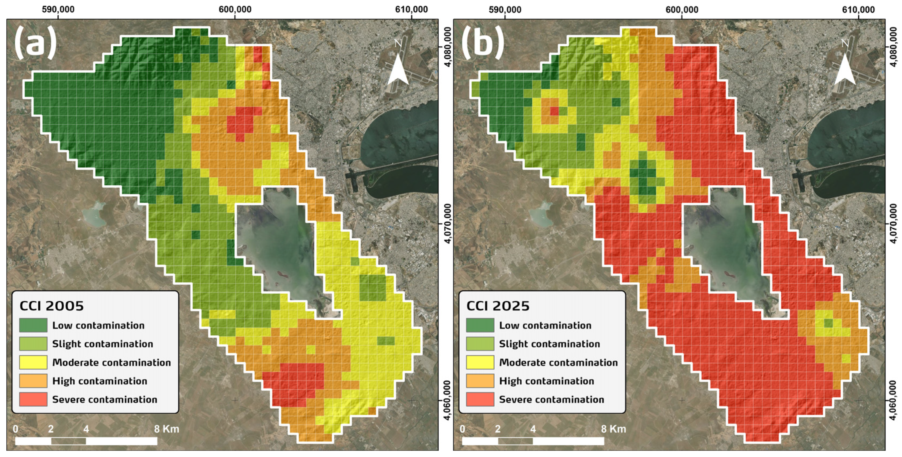
This study provides a comprehensive assessment of groundwater quality evolution in the Manouba peri-urban aquifer between 2005 and 2025, highlighting the dominant role of land transformation and anthropogenic pressures. The CCI results reveal a marked deterioration in groundwater quality over the study period, reflecting the combined effects of urban expansion and agricultural intensification.

Spatial patterns indicate that groundwater contamination is strongly structured by anthropogenic drivers rather than randomly distributed. High CCI values are concentrated in areas undergoing intensive urbanisation and cultivation, where impervious surfaces alter recharge processes and increase pollutant residence time in the subsurface [7,10,14]. Nitrate emerged as the most influential parameter controlling CCI variability, confirming the dominant role of agricultural fertilisation and urban/industrial inputs [39,43]. This apparent dominance should be interpreted in a multivariate statistical sense, as it reflects the relative contribution of nitrate within the CCI framework and its broader concentration variability, rather than implying it is the sole controlling factor of hydrogeochemical processes. In this context, other indicators such as chloride and total dissolved solids also point to concurrent salinisation processes, indicating that groundwater quality degradation results from multiple interacting anthropogenic and geogenic drivers. The spatial shift of nitrate hotspots toward more urbanised zones by 2025 reflects the evolving nature of contamination sources under progressive land transformation.

From a hydrogeochemical perspective, two main mechanisms explain the observed trends. First, urbanisation modifies the natural hydrological cycle by reducing infiltration and enhancing runoff and evapoconcentration, leading to increased solute accumulation. Second, agricultural and industrial activities contribute sustained contaminant loading, particularly nitrate and dissolved salts, resulting in progressive salinisation and localised contamination hotspots. These processes are widely documented in Mediterranean peri-urban aquifers experiencing rapid land-use change [14,15,23].

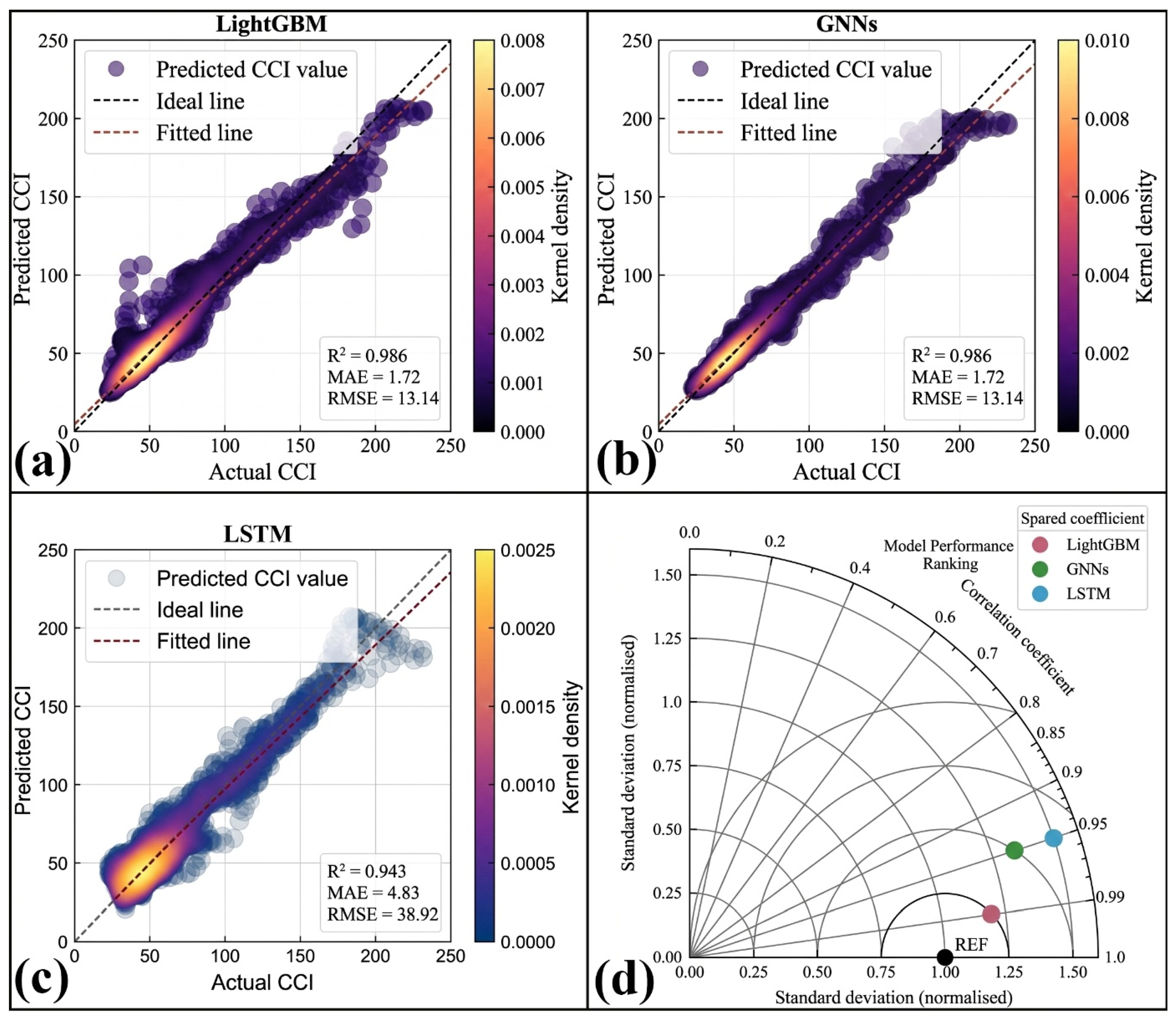
The Geo-AI ensemble framework provides further insight into these dynamics. Among the tested models, LightGBM demonstrated the highest predictive accuracy, highlighting its capacity to capture nonlinear interactions and heterogeneous hydro-chemical responses. GNNs effectively represented spatial dependencies related to hydrogeological connectivity; however, the GNN architecture is based on spatial adjacency and does not explicitly incorporate directional hydraulic gradients or groundwater flow vectors; therefore, it captures spatial connectivity patterns rather than physically constrained advective transport pathways. LSTM showed comparatively lower performance, which can be attributed both to the limited temporal resolution of the dataset (two discrete time points) and to the predominance of spatially driven contamination processes. It should be noted that deep LSTM networks are typically designed to exploit multiple sequential time steps, and their use in this study is therefore exploratory given the limited temporal sampling. This result confirms that ensemble models such as LightGBM are more suitable for the present study configuration.

A comparison with conventional groundwater quality indices, such as the Water Quality Index (WQI), highlights the added value of the proposed Composite Contamination Index (CCI). While WQI remains widely used due to its simplicity, it typically relies on fixed or expert-based weighting schemes that may not fully capture complex interactions among hydrochemical variables. In contrast, the CCI integrates subjective (BWM) and objective (CRITIC) weighting within an optimization framework, allowing a more adaptive and data-driven representation of contamination processes. Furthermore, coupling CCI with Geo-AI models enables spatial prediction and dynamic analysis, extending beyond the static assessment provided by traditional indices. This integration enhances both interpretability and predictive capability, positioning CCI as a more suitable tool for dynamic groundwater quality assessment in rapidly evolving peri-urban systems.

Although machine learning models are typically data-hungry, the present study operates with a relatively moderate dataset consisting of 295 samples distributed across 85 wells over two time periods. To mitigate the limitation of limited data availability, several strategies were adopted. First, the dataset was structured using spatially distributed samples rather than relying on a single temporal sequence, which increases the effective diversity of the training data. Second, ensemble-based and tree-based models such as LightGBM were included, as they are known to perform well with limited to moderate-sized datasets and are less prone to overfitting compared to deep neural networks.

In addition, cross-validation and appropriate regularization mechanisms were employed to ensure model generalization and robustness. Data balancing techniques such as synthetic oversampling (e.g., SMOTE) were not applied in this study, as they may introduce artificial variability in continuous hydrochemical datasets and potentially affect the physical interpretability of model outputs.

From a management perspective, the findings provide important implications for groundwater protection. Urban planning should incorporate strategies to preserve recharge zones and limit excessive soil sealing. At the same time, improved regulation of agricultural practices and wastewater management is essential to control nitrate inputs and mitigate salinisation. The integration of grid-based monitoring with AI-driven predictive tools offers a promising approach for early detection of contamination trends and adaptive groundwater management.

It should be emphasized that the methodology does not assume temporal stationarity of groundwater contamination. The 2005 and 2025 datasets represent two independent snapshots of the aquifer system, and the observed differences reflect real temporal changes driven by evolving anthropogenic and environmental conditions, rather than a constant underlying contamination state. It should also be acknowledged that land-use practices, irrigation strategies, and regulatory frameworks may have evolved between the two periods. However, these changes are implicitly reflected in the observed spatial differences, as the study treats each year as an independent snapshot rather than modeling continuous temporal transitions.

A key limitation of this study lies in both the sampling design and the spatial aggregation approach. Groundwater samples collected in 2005 and 2025 originate from partially overlapping but non-identical sets of monitoring wells, meaning that the 2025 dataset does not represent a strict subset of the 2005 network. This prevents direct paired comparisons at identical locations and introduces uncertainty in point-based temporal interpretation. Consequently, temporal variations are evaluated at the level of spatial distributions rather than point-based trajectories. In addition, the dataset exhibits uneven temporal density, with more extensive sampling in 2005 than in 2025, as well as a non-uniform spatial distribution of wells. To address these constraints, hydrochemical parameters and CCI values were aggregated within a 500 m × 500 m grid framework, enabling consistent regional-scale comparison between the two periods. Although high-precision GPS coordinates were available for individual wells, the chosen grid resolution represents a compromise between spatial accuracy and data density, ensuring robust interpolation while maintaining consistency with the sampling distribution. However, this aggregation may smooth local variability and partially mask small-scale contamination hotspots, which are particularly relevant in peri-urban environments characterized by heterogeneous pollution sources. Similarly, the aggregation of land-use information at the pixel level (18 × 18) may also reduce high-frequency spatial variability associated with localized urban-industrial contamination sources, although this trade-off was necessary to reduce local noise and ensure consistency with the scale of hydrochemical observations. Despite this limitation, the combined use of geostatistical interpolation and spatial modelling preserves the dominant contamination gradients and allows robust identification of regional patterns. Future studies should incorporate higher-resolution sampling strategies and denser monitoring networks to better capture fine-scale heterogeneity and localized contamination processes.

Future work should focus on increasing sampling density, incorporating multi-temporal monitoring datasets, and integrating additional tracers such as emerging contaminants and isotopic indicators. It should be noted that the present study is limited to inorganic hydrochemical parameters, while emerging contaminants were not included in the analysis and are considered as a direction for future research rather than part of the current dataset. These improvements would enhance both process understanding and the predictive capability of Geo-AI frameworks, supporting more robust groundwater management in peri-urban environments.

Another avenue for improvement concerns the integration of physical hydrological processes into the modelling framework. Incorporating groundwater flow information, such as Darcy-based flow vectors, into the graph structure of GNN models could enhance the representation of contaminant transport pathways. However, such an approach requires detailed hydraulic and piezometric data, which were not available for the full study period. Future work should explore hybrid modelling strategies combining data-driven approaches with physically based constraints to improve process realism.

More advanced hybrid modeling approaches, such as Physics-Informed Neural Networks (PINNs), offer a promising avenue to further enhance groundwater modeling by embedding physical laws directly into the learning process through physics-based constraints in the loss function. Such approaches have recently been applied in groundwater and water resources studies and hydrogeological studies to improve model generalization, particularly in data-scarce contexts. However, the implementation of PINNs typically requires well-defined governing equations and additional calibration of physical parameters, which are beyond the scope of the present study. Future work could explore the integration of physics-informed learning frameworks to further improve predictive performance and physical consistency of groundwater quality models [52,53,54].

7. Conclusions

This study presents a comprehensive assessment of groundwater quality in the Manouba peri-urban aquifer between 2005 and 2025 by integrating hydrochemical analyses, land-change dynamics, and advanced machine-learning approaches. The Composite Contamination Index (CCI) revealed a clear deterioration of groundwater quality over the study period. In 2005, groundwater conditions were relatively balanced, with low contamination covering 25% of the area and slight contamination 20%, while moderate, high, and severe contamination accounted for 30%, 18%, and 7%, respectively. By 2025, the spatial distribution of CCI classes shifted markedly toward more degraded conditions. Severe contamination became dominant, representing 55% of the area, followed by high contamination (15%) and moderate contamination (10%), whereas slight and low contamination declined to 12% and 8%, respectively. This evolution highlights the progressive expansion of highly contaminated zones within the aquifer system.

Machine-learning analyses demonstrated the effectiveness of advanced algorithms in modelling complex interactions between hydrochemical variables and land changes. Among the tested models, LightGBM achieved the highest predictive performance, with R² = 0.986, RMSE = 13.14, and MAE = 1.72 for CCI prediction. GNNs also showed strong predictive capability (R² = 0.972, RMSE = 18.73, MAE = 2.11), particularly in capturing spatial dependencies related to hydrogeological connectivity. In contrast, LSTM exhibited comparatively lower accuracy (R² = 0.943, RMSE = 38.92, MAE = 4.83), reflecting the predominantly spatial rather than temporal nature of groundwater contamination processes. Residual analyses further confirmed that LightGBM and GNNs produced stable and largely unbiased predictions across the contamination spectrum, whereas LSTM displayed greater dispersion near CCI threshold boundaries.

Variable importance and sensitivity analyses highlighted the dominant influence of artificial surfaces and cultivated lands, which explained most of the spatial and temporal variability in CCI. Other land-cover types, including forests, wetlands, shrublands, and water bodies, contributed marginally due to their limited spatial extent. These results demonstrate that urban expansion and agricultural intensification are the principal drivers of groundwater degradation in the Manouba aquifer.

Two major mechanisms explain the influence of urbanisation on groundwater quality. First, the conversion of natural or agricultural land into artificial surfaces modifies recharge, flow, and discharge processes, leading to increased concentration of hydrochemical parameters in certain zones. Second, the concentration of industrial and urban activities in pollution-intensive areas further increases groundwater vulnerability, particularly to nitrate contamination.

The integration of hydrochemical monitoring, CCI-based contamination assessment, land-change analysis, and machine-learning modelling provides a robust framework for understanding groundwater quality evolution under increasing anthropogenic pressure. The results clearly indicate a progressive shift toward higher contamination levels between 2005 and 2025, with severe contamination expanding across large parts of the aquifer. Among the evaluated models, LightGBM emerged as the most reliable predictive framework, offering high accuracy and stability under heterogeneous hydrochemical conditions. These findings provide a strong scientific basis for improving groundwater management, guiding sustainable land-use planning, and implementing targeted pollution mitigation strategies in the Manouba region and in similar peri-urban aquifer systems.