A Detailed Simulation of Overtopping-Induced Breach Processes and Breach Evolution in Non-Cohesive Earth Dams

Abstract

Non-cohesive earth dams are widely distributed in natural and semi-engineering scenarios, and overtopping-induced breaches are their most catastrophic failure mode. Accurate prediction of the overtopping failure process and breach evolution is critical for risk assessment, emergency management, and dam design optimization. In this study, an improved 3D numerical method is developed to simulate the coupled hydrodynamic–erosion–breach evolution processes of non-cohesive earth dams. The model based on the finite volume method integrates three core modules: a hydrodynamic module based on the Reynolds-Averaged Navier–Stokes equations with the Volume of Fluid method for free surface tracking, a dam material erosion module considering particle entrainment and transport mechanisms of non-cohesive soils, and a breach development module coupling erosion and gravitational collapse. To validate the model, two levels of verification are conducted: first, a classic benchmark dam break case is employed to confirm the feasibility of the hydrodynamic and breach evolution algorithms; second, published flume experimental data of non-cohesive earth dam overtopping failures are adopted to evaluate the model accuracy in predicting breach hydrographs and spatiotemporal evolution of breach geometry. The results demonstrate that the proposed model accurately reproduces the key characteristics of overtopping failure with high fidelity. The predicted breach flow rates and flow depths are in excellent agreement with experimental observations, with relative errors less than 5% for both peak discharge and time to peak. Consequently, this study provides a reliable numerical tool for detailed simulation of non-cohesive earth dam breaches and offers scientific support for emergency management.

1. Introduction

Non-cohesive earth dams, such as landslide dams or debris flow-induced dams, which are composed of sand, gravel, or gravel-sand mixtures, are widely formed by post-semi river blocking or temporary water impoundment. Their inherent low resistance to erosion makes them highly vulnerable to overtopping failure [1]. According to statistics of 245 landslide dam breach cases, over 90% of dam failure incidents are triggered by overtopping [2]. When a dam breaches, the sudden release of impounded water forms a breach flood that propagates downstream at high velocity, resulting in devastating flash floods downstream. In 2018, the Baige landslide dam in China experienced two overtopping-induced breaches, which affected more than 100,000 people in total, and the peak discharge reached 31,000 m³/s [3]. Therefore, understanding the mechanisms of overtopping failure and accurately predicting breach evolution are essential for mitigating such risks.

Dam breach research relies on three main approaches: field observations, physical model experiments, and numerical simulations [4,5]. Field observations are limited by the rarity and unpredictability of natural dam failures, making it difficult to obtain systematic data on the entire failure process [6]. Laboratory-scale models cannot fully replicate the grain size distribution, flow turbulence, and erosion dynamics of prototype dams and require specialized facilities and intensive monitoring, making them impractical for parametric studies [7]. In contrast, numerical simulation overcomes these drawbacks by reproducing the fully physical process of overtopping, enabling parametric sensitivity analysis, and providing real-time spatiotemporal data (e.g., velocity fields in the breach, erosion rates of dam material, and flow depths downstream) that are difficult to obtain experimentally. Thus, a reliable detailed numerical model is critical for risk assessment and emergency response planning.

The numerical model for a dam breach can generally be categorized into three types: empirical models and physically based simplified and detailed models [8]. The early dam breach empirical models focused on simplified estimation of key breach parameters using empirical formulas derived from historical failure cases [9,10,11]. These models exhibit high computational efficiency but lack a physical theoretical basis, failing to simulate the transient interaction between water flow and dam material, and they thus cannot accurately capture the breach hydrograph. For the aforementioned reasons, scholars worldwide have developed some physically based simplified models based on dam breach mechanisms, which have become the mainstream approach for calculations (e.g., the DLBreach model [12], DB-IWHR model [13] and DB-NHRI model [14]). Unlike empirical models, these simplified models can typically output the breach hydrograph and breach morphology evolution. These models assume an initial trapezoidal breach shape and adopt the wide-crested weir discharge formula and sediment erosion formula to simulate the dam breach process [15]. Although this approach improves physical realism, it is still limited by dimension reduction and simplified erosion mechanisms, failing to achieve detailed simulation of the dam breach process and dynamics of breach flow.

With the development of computational fluid dynamics (CFD) and soil mechanics, a series of physically based detailed numerical methods for the dam breach process have been established based on the theories of hydrodynamics and sediment transport. Typically, such numerical models are founded on the Navier–Stokes equations and consist of three core modules, namely, the hydrodynamic module, dam material erosion module, and breach morphology evolution module. Early detailed models were mostly based on the Saint-Venant equations and employed hydrodynamic models for calculation after deriving the breach discharge via empirical formulas [16]. However, they are mostly applicable only to open-channel flows with low velocity and homogeneous granular materials and cannot adequately simulate the dam material erosion behavior under complex flow conditions. The existing 1D cross-sectional averaged and 2D depth-averaged dam break mathematical models are generally based on the hydrostatic pressure distribution assumption and have not yet involved the simulation of 3D failure processes of earth dams [17,18]. Meanwhile, during the dam breach process, the released flow carries a large amount of sediment downstream, exhibiting distinct turbulent characteristics. In contrast, the wide-crested weir discharge formulas adopted in existing dam break hydrodynamic models and simplified numerical models are mostly based on the laminar flow assumption, which cannot properly describe the complex flow patterns of dam break flows. In addition, the scouring induced by dam break flows can lead to the bed undermining and the instability of breach slopes [19]. Meanwhile, the breach morphology evolution also affects the hydrodynamic characteristics of dam break flows. Therefore, it is important to consider the coupling relationship between breach flows, dam material erosion, and breach morphology in numerical simulations.

Therefore, this study establishes an improved 3D numerical method that integrates a hydrodynamic model, turbulent flow governing equations, and an erosion model with fractional transport calculation for different particle groups in wide-graded geomaterials. In addition, the model uses an optimized sub-time-step iteration algorithm that couples flow–sediment calculation and gravitational collapse within the same computational cycle, solving the temporal inconsistency problem in our previous model and better reproducing the synchronous vertical deepening and lateral widening of the breach. Typical benchmark test cases under movable-bed conditions and flume experiments are selected to verify the applicability of the numerical model.

2. Three-Dimensional Detailed Numerical Model

The proposed numerical model consists of three modules: hydrodynamic, dam material erosion, and dynamic breach evolution.

2.1. Hydrodynamic Module

The module simulates transient, incompressible, turbulent water flow using the three-dimensional Reynolds-Averaged Navier–Stokes (RANS) equations and the Volume of Fluid (VOF) method for tracking the air–water free surface [20]. The continuity equation and momentum equation are presented as follows:

$${\displaystyle \frac{\partial \rho }{\partial t}}+\nabla \cdot (\rho \mathbf{u}) = 0$$

(1)

where ρ is the fluid density (kg/m³), t is time (s), and u = (u, v, w) is the velocity vector (m/s) in the x, y, and z directions.

$${\displaystyle \frac{\partial (\rho \mathbf{u})}{\partial t}}+\nabla \cdot (\rho \mathbf{uu})= -\nabla p+\nabla \cdot ({\mu }_{\mathrm{eff}}(\nabla \mathbf{u}+\nabla {\mathbf{u}}^T\left)\right)+\rho \mathbf{g}+{\mathbf{F}}_{\mathrm{int}}$$

(2)

where p is the static pressure (Pa), μ_eff = μ + μ_t is the effective dynamic viscosity (Pa·s), μ is the molecular viscosity (Pa·s), μ_t is the turbulent viscosity (Pa·s), with μ_t = ρC_μk²/ε, where C_μ = 0.085 is the empirical constant of the turbulence model calibrated for high-shear free-surface flows, k is the turbulent kinetic energy, ε is the turbulent dissipation rate, and g is the gravitational acceleration vector (m/s²), and F_int is the interfacial force between air and water calculated via the VOF method.

The VOF method defines a volume fraction of water α (0 < α < 1), where α = 1 indicates a cell fully filled with water, α = 0 indicates a cell filled with air, and 0 < α < 1 indicates the interface. The transport equation for α is [21]:

$${\displaystyle \frac{\partial \alpha }{\partial t}}+\nabla \cdot (\alpha \mathbf{u}) = 0$$

(3)

Furthermore, the RNG k-ε model is selected for simulating turbulence, as it is well-suited for high-shear flows, like the breach region of dams, and accounts for the effects of streamline curvature [22]. The model solves transport equations for turbulent kinetic energy and the turbulent dissipation rate:

$${\displaystyle \frac{\partial (\rho k)}{\partial t}}+\nabla \cdot (\rho \mathbf{u}k) = \nabla \cdot ({\alpha }_k{\mu }_{\mathrm{eff}}\nabla k)+G_k-\rho \epsilon$$

(4)

$${\displaystyle \frac{\partial (\rho \epsilon )}{\partial t}}+\nabla \cdot (\rho \mathbf{u}\epsilon )=\nabla \cdot ({\alpha }_{\epsilon }{\mu }_{\mathrm{eff}}\nabla \epsilon )+C_{1\epsilon }{\displaystyle \frac{\epsilon }{k}}{G}_k-C_{2\epsilon }\rho {\displaystyle \frac{{\epsilon }^2}{k}}+R_{\epsilon }$$

(5)

where G_k is the turbulent kinetic energy production term due to mean velocity gradients, with G_k = μ_t(∇u + ∇u^T):∇u, R_ε is the RNG correction term accounting for streamline curvature, with R_ε = C_μη(1 − η/η₀)ρε²/[(1 + βη³)k], where η = Sk/ε, S is the module of the mean strain rate tensor, and η₀ = 4.38, β = 0.012, α_k = 1.0, α_ε = 1.3, C_1ε = 1.44, C_2ε = 1.92 are the empirical constants of the RNG k-ε model.

2.2. Dam Material Erosion Module

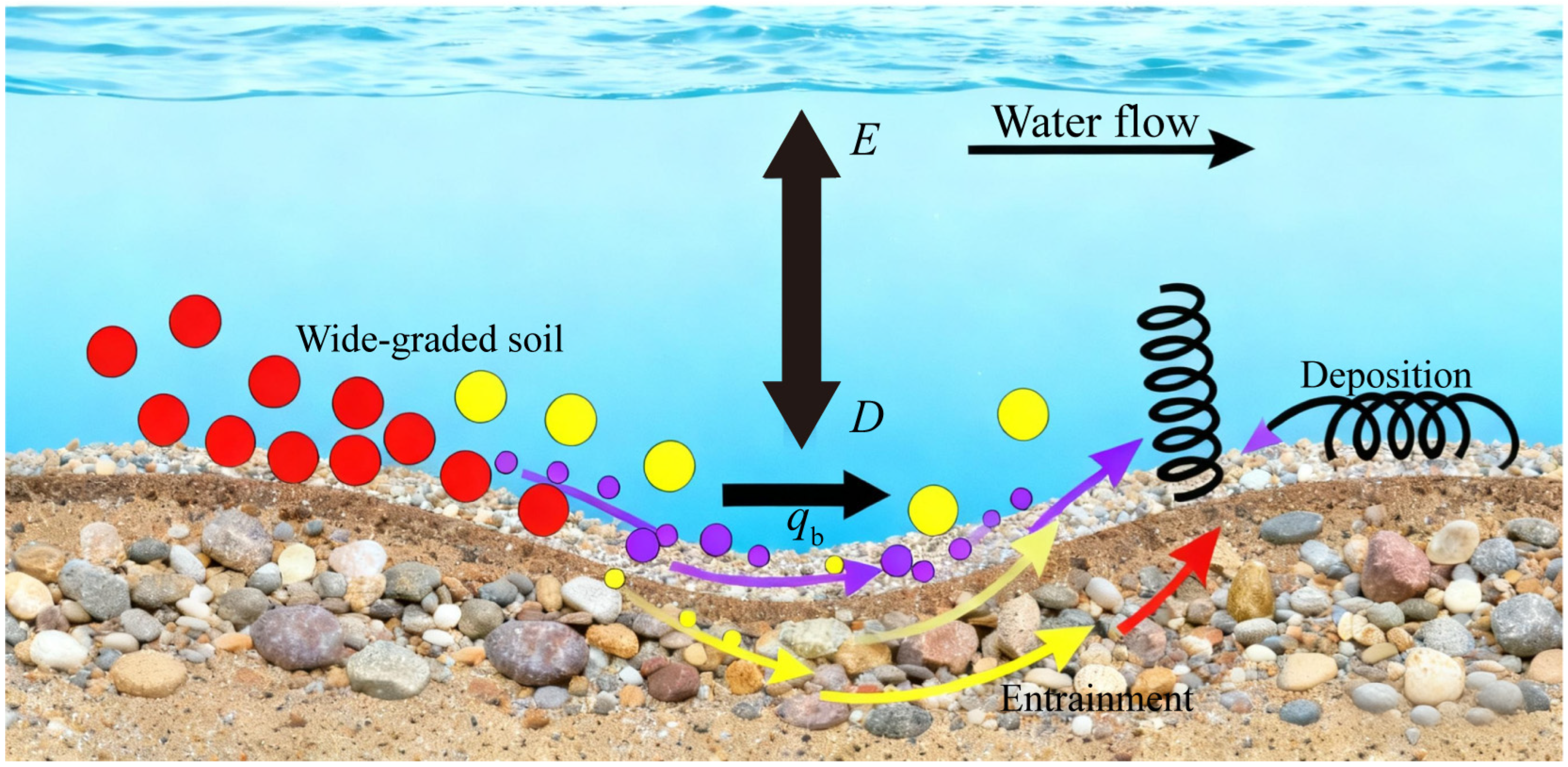
Non-cohesive soil erosion during overtopping failure is dominated by hydraulic entrainment: the flow shear stress acting on the dam surface exceeds the critical shear stress of the soil particles, leading to particle detachment and transport. As shown in Figure 1, the entrainment (E) and deposition (D) of dam material can be regarded as two opposite micro-processes, and the net exchange rate between bedload and suspended load can be obtained through comprehensive calculation [23].

Considering the distinct erodibility traits of heterogeneous components within dam materials, the entrainment lift rate is applied to quantify the amount of transported material converted into suspended material [24].

$$E_i={\alpha }_i{n}_s{d}_{\ast ,i}^{0.3}({\theta }_i-{\theta }_{\mathrm{cr},i}{)}^{1.5}{\left[g\left({\displaystyle \frac{{\rho }_{s,i}-{\rho }_w}{{\rho }_w}}\right)d_i\right]}^{0.5}$$

(6)

where α_i denotes the entrainment coefficient of different component materials; n_s is the normal vector of the filling bed at the breach; d_∗,i represents the dimensionless particle size parameter of each component material, with d_∗,i = d_i(ρ_w(ρ_s,I − ρ_w)g/μ²)^1/3; θ_i is the dimensionless Shields number, which can be calculated based on the critical shear stress τ_c with θ_i = τ_c/(gd_i(ρ_s,i − ρ_w)) and τ_c = ρ_igu²/C_D, where C_D is the drag coefficient related to the averaged particle size, with C_D = 5.75 g^0.5log(2h/d₅₀); θ_cr,i is the critical dimensionless Shields number for particle entrainment of the i-th particle group; ρ_s is the soil density; ρ_w is the water density; and d_i is the representative particle size of each component material.

The deposition rate of dam sediment characterizes the process by which particles settle out of the suspended load and deposit onto the bedload layer under gravitational effects [25].

$$D_i={\omega }_i{C}_{s,i}$$

(7)

$${\omega }_i={\displaystyle \frac{v_i}{d_i}}[(10.36^2+1.049d_{\ast ,i}^3{)}^{0.5}-10.36]$$

(8)

where ω_i is the effective settling velocity; C_s,i is the mass concentration of the suspended load; and ν_i is the kinematic viscosity of the fluid.

Given the wide gradation characteristics of non-cohesive earth dams, modified Meyer–Peter and Muller’s empirical formulas are adopted [26]:

$$q_{\mathrm{b},i}=K{\left({\theta }_i-{\theta }_{\mathrm{cr},i}\right)}^{1.5}{\left[\mathrm{g}\left({\displaystyle \frac{{\rho }_{\mathrm{s},i}-{\rho }_{\mathrm{w}}}{{\rho }_{\mathrm{w}}}}\right)d_i^3\right]}^{0.5}$$

(9)

where q_b is the volumetric bedload transport rate per unit width, and K is the bedload coefficient.

The total single-width sediment transport rate (q_bt) is calculated by summing the individual component rates (q_bt,i) based on their respective proportions (f_i).

$$q_{\mathrm{bt}}=\sum _{i=1}^k{q}_{\mathrm{b},i}{f}_i$$

(10)

Finally, the concentration of suspended particles is calculated by the convection diffusion equation and can be expressed as [27]:

$${\displaystyle \frac{\partial C_{\mathrm{s},i}}{\partial t}}+\nabla ·(u_{\mathrm{s},i}\hspace{0.17em}{C}_{\mathrm{s},i})=\nabla ·\nabla (\xi \hspace{0.17em}{C}_{\mathrm{s},i})$$

(11)

where C_S,i denotes the mass concentration of suspended sediment for each constituent material, representing the sediment mass per unit volume of the fluid–sediment mixture; ξ represents the diffusion coefficient of suspended sediment; u_s,i is the suspended flow velocity of different dam material with u_s,i = u_m + ω_ic_s,i, in which u_m is the velocity of the fluid–sediment mixture, and c_s,i is the volume concentration of suspended mass of dam material with different components.

2.3. Breach Development Module

According to the non-cohesive earth dam overtopping-induced breach mechanisms obtained from field observation and experimental research [6,14], the breach morphology evolution is dynamically updated via the intense interaction between hydrodynamic regimes and the breach boundary, which mainly includes: vertical deepening driven by erosion of the dam crest and breach bottom and lateral widening due to the breach sidewall erosion and gravitational collapse.

Dam material transport along the flow direction induces scour and deposition of the bed surface, and the breach elevation is determined via mass conservation equations governing the deposited sediment bed, suspended load and bed load [19].

$${\varphi }_{\mathrm{s}}{\displaystyle \frac{\partial z_{\mathrm{b}}}{\partial t}}=({\displaystyle \frac{\partial q_{\mathrm{tx}}}{\partial x}}+{\displaystyle \frac{\partial q_{\mathrm{ty}}}{\partial y}}+D-E)$$

(12)

where ϕ_s is the sediment volume fraction; and q_tx and q_ty are the total sediment transport rates in the x and y directions, respectively.

The moving interface between the fluid and dam material is reconstructed and simulated using the VOF method. The volume fraction of dam material is derived by tracking the bed load and suspended load concentrations computed by the dam material erosion module:

$${\varphi }_{\mathrm{s}}={\displaystyle \frac{C_{\mathrm{b},i}+C_{\mathrm{s},i}}{{\rho }_{\mathrm{s}}}}=1-{\varphi }_{\mathrm{f}}$$

(13)

where ϕ_f is the fluid volume fraction.

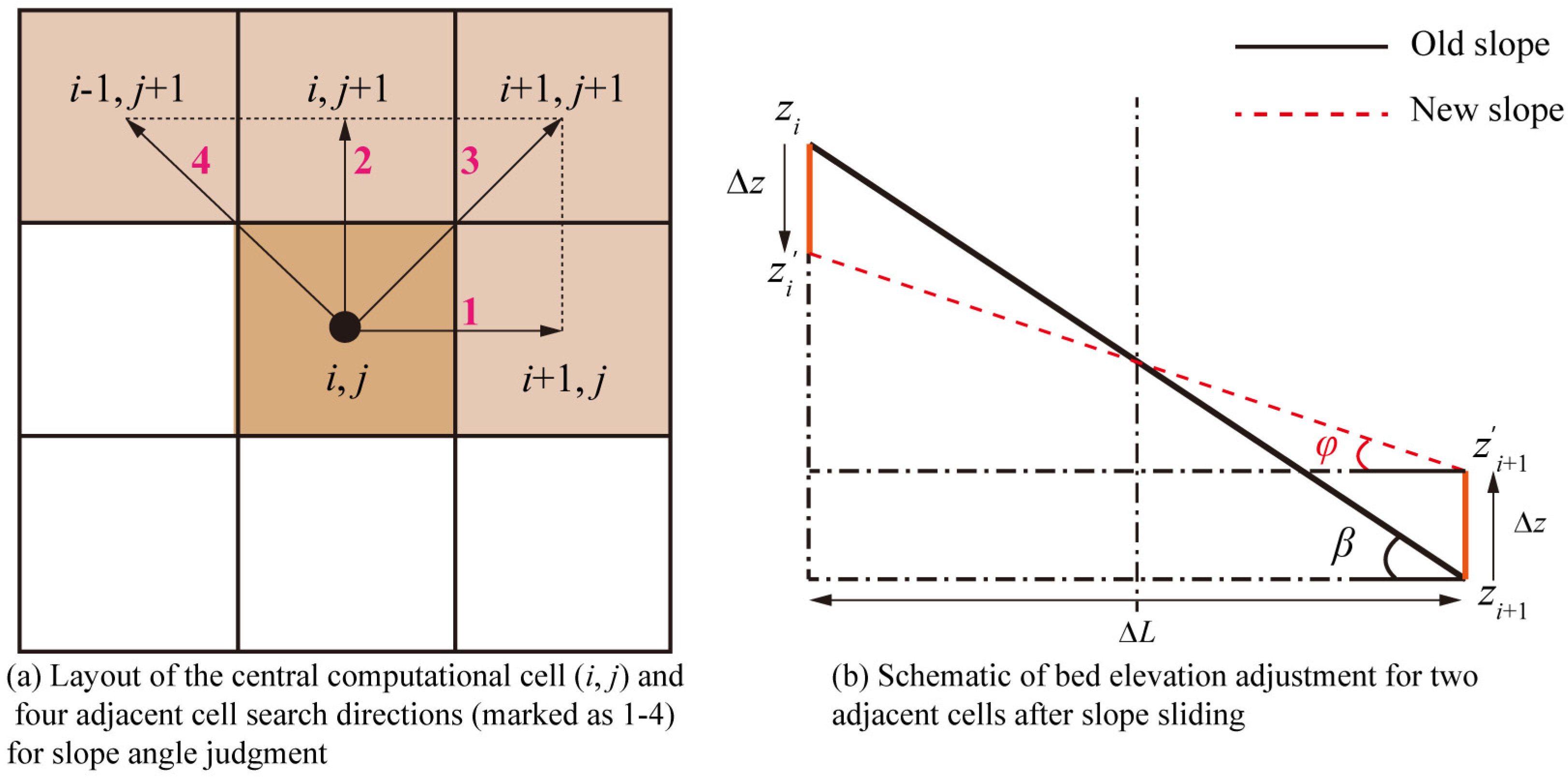
The breach development module needs to consider not only flow-induced forces but also the mechanical properties of dam materials. It is assumed that slope instability occurs when the slope angle of the breach sidewall exceeds or equals the angle of repose of the dam material. It should be noted that this stability criterion is a simplification, which is adopted because the initial focus of this study is on the rapid breach evolution of fully saturated non-cohesive granular materials, where the effect of transient pore water pressure is assumed to be secondary. To simulate the slope sliding process, the principle of mass conservation for dam materials is strictly followed while satisfying the aforementioned instability criterion. By lowering cells at higher elevations and raising those at lower elevations, the slope angle of the updated breach is made approximately equal to the angle of repose (see Figure 2). Subsequently, the temporal evolution of both the breach top width and bottom width can then be derived using the breach depth and the angle of repose.

$$\left\{\begin{array}{l}{z}_i^{\prime }=z_i-\Delta z\\ z_{i+1}^{\prime }=z_{i+1}+\Delta z\end{array}\right.$$

(14)

$$\Delta z={\displaystyle \frac{\Delta L(\tan \beta -\tan \varphi )}{2}}$$

(15)

where z_i′ and z_i+1′ are the breach bed elevation of the i-th and (i + 1)-th cells after sliding, respectively; z_i and z_i+1 are the breach bed elevations of the i-th and (i + 1)-th cells before sliding, respectively; Δz is the variable of breach bed elevation caused by sliding; ΔL is the distance between the centers of two adjacent cells; β is original breach slope angle; and $\varphi$ is the angle of repose.

The coupling between the flow–sediment time step and the slope stability criterion is achieved through a sub-time-step iteration within each computational cycle. Specifically, at the end of each flow–sediment time step, the hydrodynamic conditions are first updated, and the breach slope angle of all sidewall cells is calculated. Then, it is checked whether the slope angle meets the instability criterion. If satisfied, the slope sliding process is executed iteratively until the slope angle is reduced to approximately the angle of repose. This sub-time-step iteration ensures that gravitational collapse is resolved within the same computational time step as flow and erosion calculations, maintaining temporal consistency and numerical stability.

2.4. Numerical Algorithm

In this study, the governing equations are discretized using the finite volume method (FVM) due to its conservation properties, and the control equations of the above hydrodynamic and dam material transport mathematical models can be written in a general form:

$${\displaystyle \frac{\partial \varphi }{\partial t}}+\mathrm{div}\left(U_{\varphi }\right)-\mathrm{div}\left({\Gamma }_{\varphi }\cdot \mathrm{grad}\varphi \right)=S_{\varphi }$$

(16)

where ϕ is a general variable; U is the velocity vector; Г_ϕ is the diffusion coefficient of the variable; and S_ϕ is the source term.

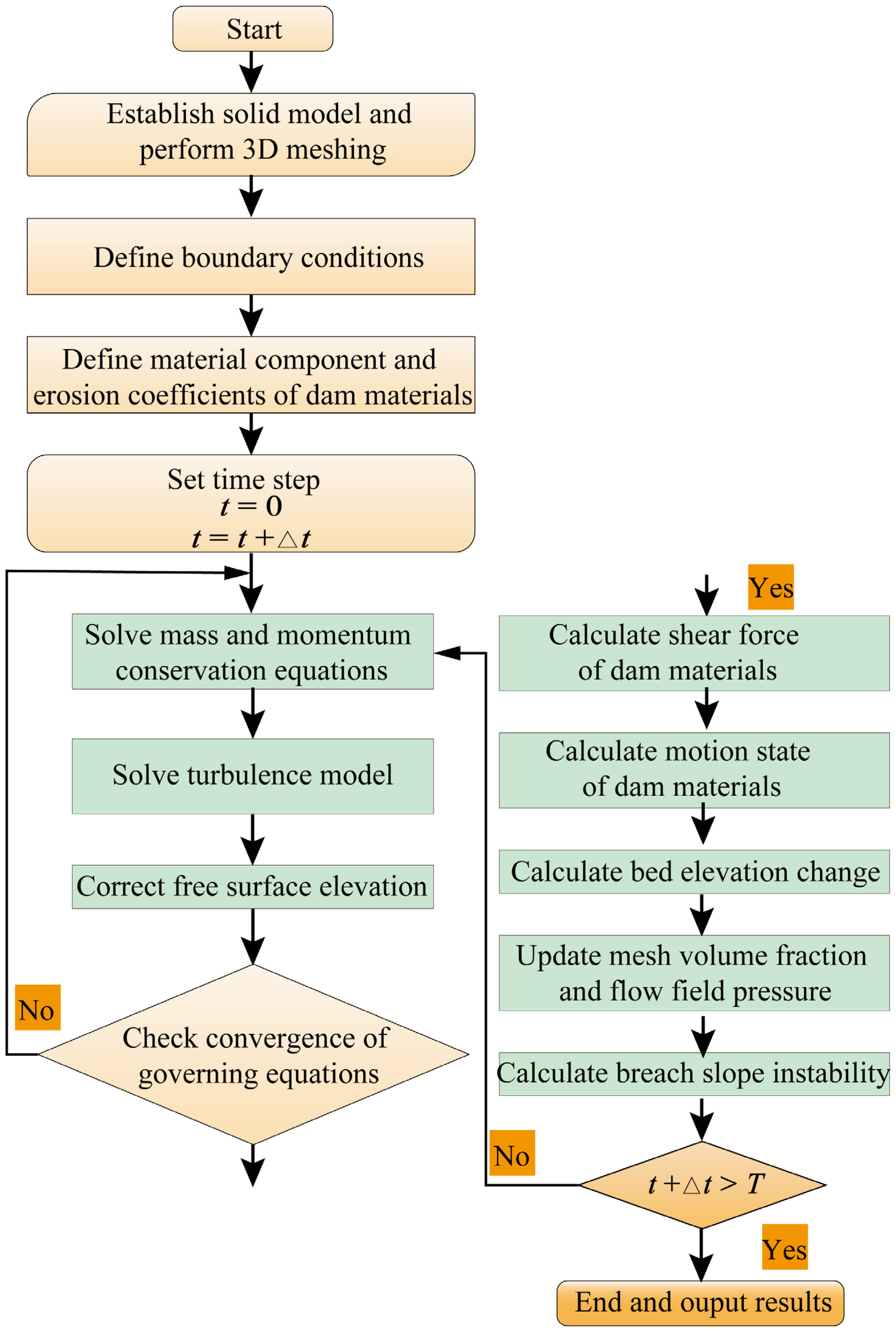
Figure 3 depicts the calculation flowchart of the numerical model. For time discretization, the first-order implicit Euler scheme for transient terms is suitable for long-duration simulations. For spatial discretization, the third-order QUICK scheme is used for velocity to reduce numerical diffusion at the air–water interface. The second-order central differencing scheme is selected for viscosity and turbulence terms. The PIMPLE algorithm (a combination of PISO and SIMPLE) is used to solve the coupled RANS-VOF equations, which balances accuracy and computational efficiency. The computational domain is discretized into structured grid cells, with each cell storing the integral average values of relevant dependent variables. Meanwhile, the Fractional Area Volume Obstacle Representation (FAVOR) method is employed to resolve complex geometric solid regions [28]. When simulating complex structures, this method enables the representation of arbitrary complex geometrics using simple rectangular grids, facilitating easy grid generation and ensuring high numerical accuracy.

The time step (Δt) is constrained by the Courant–Friedrichs–Lewy number (CFL ≤ 0.5) to avoid numerical instability:

$$\Delta t<N_{\mathrm{CFL}}·\min \left({\displaystyle \frac{V_{\mathrm{f}}\Delta x_i}{A_{x}u}},{\displaystyle \frac{V_{\mathrm{f}}\Delta y_j}{A_{y}v}},{\displaystyle \frac{V_{\mathrm{f}}\Delta z_{\kappa }}{A_{z}w}}\right)$$

(17)

where (u, v, w) represent the velocity amplitudes. For incompressible flow, a value of 0.25 is typically adopted for N_CFL to ensure computational stability.

3. Model Calibration via a Benchmark Case

3.1. Benchmark Case Setup

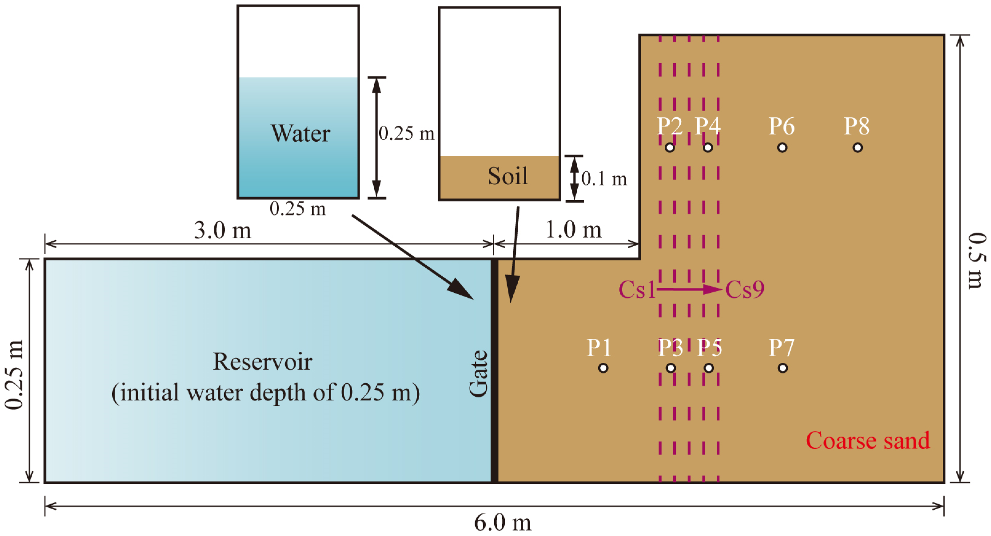
In this study, a movable-bed dam breach test case in a sudden-expansion open channel conducted in UCL-Belgium was selected as a typical benchmark case [29]. Measured experimental data were utilized to verify the applicability of the proposed model. The experimental flume has a total length of 6.0 m, with an upstream reservoir width of 0.25 m and a downstream channel width of 0.5 m. The flume width suddenly expands from 0.25 m to 0.5 m at 4.0 m from the left side (as shown in Figure 4). A gate is installed at 3.0 m from the left side of the flume. At t = 0 s, the instantaneous dam breach flow was simulated by rapidly lifting the gate, which propagates downstream. The flume bottom is paved with a 0.1 m thick layer of saturated coarse sand, serving as the erodible sediment bed. The coarse sand is uniformly graded with a mean particle size d₅₀ = 1.82 mm, density ρ_s = 2.68 g/cm³, and porosity p_m = 0.47. The initial flow depth of the upstream reservoir was set to 0.25 m, while the downstream channel is a dry bed with an initial flow depth of 0.0 m. Eight ultrasonic water level transducers (P1~P8) were arranged in the flume downstream to monitor water levels throughout the experiment, with the specific coordinates of the measured points presented in

Table 1. Coordinate information of water level gauge measuring points.

Number	X Coordinates (m)	Y Coordinates (m)
P1	3.75	0.125
P2	4.20	0.375
P3	4.20	0.125
P4	4.45	0.375
P5	4.45	0.125
P6	4.95	0.375
P7	4.95	0.125
P8	5.45	0.375

. Meanwhile, bed elevation changes at nine cross-sections (Cs1~Cs9) were surveyed at intervals of 0.05 m over the 1.1~1.5 m range downstream of the gate.

The computational domain was discretized using a three-dimensional structured grid. A systematic pre-simulation verification with three sets of uniform grid resolutions (0.004 m, 0.005 m, and 0.006 m) was conducted. The pre-simulation results show that the 0.005 m grid can accurately capture the core characteristics of dam break wave propagation, bed scouring and deposition, achieving the optimal balance between simulation accuracy and computational efficiency. Therefore, a uniform grid with a resolution of 0.005 m × 0.005 m × 0.005 m was adopted for this benchmark case. An adaptive time step was adopted in the simulation, and the total simulation duration was 12 s, consistent with the actual experiment. The Manning roughness coefficient for the entire computational domain was set to 0.025 s·m^−1/3. Solid wall boundaries were applied to the y-direction sidewalls and the bottom of the computational domain, a free outflow boundary was adopted at the downstream boundary (x = 6.0 m), and an atmospheric pressure boundary was used at the top of the domain.

3.2. Results and Discussion

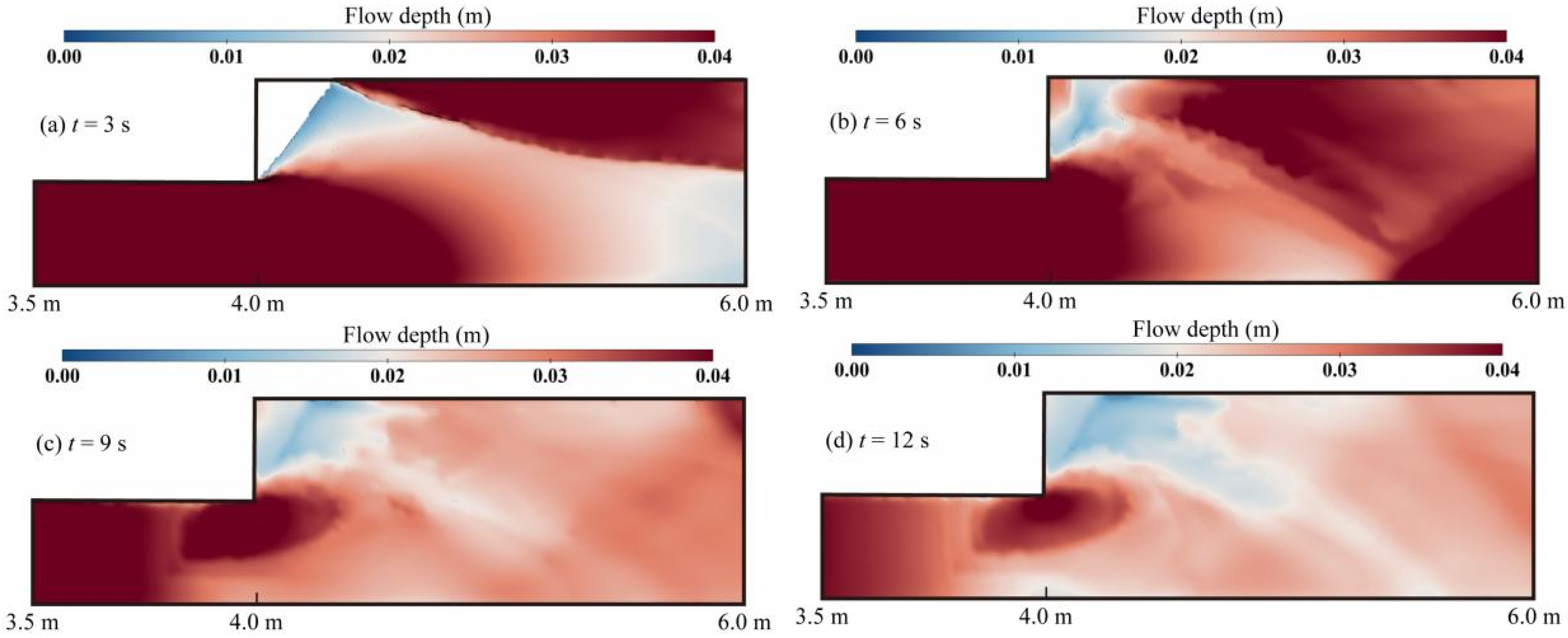
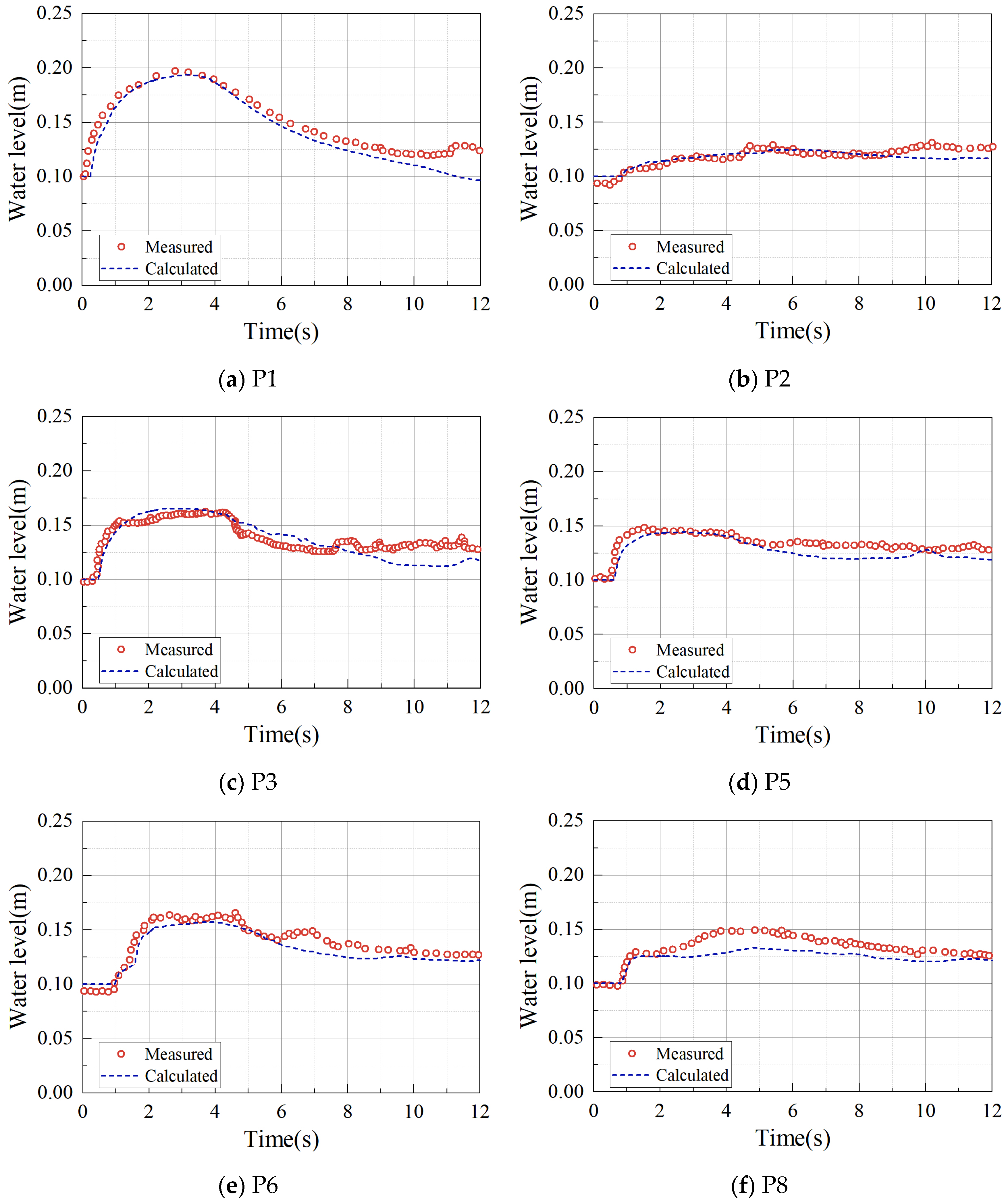
Figure 5 illustrates the calculated flow depth distributions at various time instants. As revealed in the figure, dam break flow generates a triangular vortex in the abrupt expansion region of the flume. Oblique flow is generated due to the reflection of the flow after impacting the flume sidewalls, which is basically consistent with the physical laws of actual experimental flow regimes. Commencing at t = 9 s, a vortex-like flow depth distribution is distinctly visualized at the corner points of the sudden expansion region, where the darker color indicates significant sediment scouring at the bed surface. Six representative measuring points (P1, P2, P3, P5, P6, and P7) were selected to calculate the water levels, and the numerical results were benchmarked against the experimental measurements (as shown in Figure 6).

To quantitatively evaluate the simulation performance of the hydrodynamic module, the Root Mean Square Error (RMSE), Nash–Sutcliffe Efficiency (NSE), and Percent Bias (PBIAS) are selected as the core statistical indicators, which are defined as:

$$RMSE=\sqrt{{\displaystyle \frac{1}{N}}\sum _{i=1}^N{\left(x_{\mathrm{sim},i}-x_{\mathrm{mea},i}\right)}^2}$$

(18)

$$NSE=1-{\displaystyle \frac{{\sum }_{i=1}^N{\left(x_{\mathrm{sim},i}-x_{\mathrm{mea},i}\right)}^2}{{\sum }_{i=1}^N{\left(x_{\mathrm{mea},i}-{\stackrel{-}{x}}_{\mathrm{mea}}\right)}^2}}$$

(19)

$$PBIAS={\displaystyle \frac{{\sum }_{i=1}^N{x}_{\mathrm{mea},i}-x_{\mathrm{sim},i}}{{\sum }_{i=1}^N{x}_{\mathrm{mea},i}}}\times 100$$

(20)

where N is the total number of time-series data points, x_sim,i is the simulated data at the i-th time step, x_mea,i is the corresponding measured data, and ${\stackrel{-}{x}}_{\mathrm{mea}}$ is the arithmetic mean of all measured values.

The statistical results show that the average RMSE of the water level across all monitoring points is 0.012 m, with the maximum RMSE of 0.016 m at point P6 and the minimum RMSE of 0.009 m at point P1. These quantitative results further confirm that the proposed model can accurately simulate the hydrodynamic behaviors of dam break flow under movable-bed conditions.

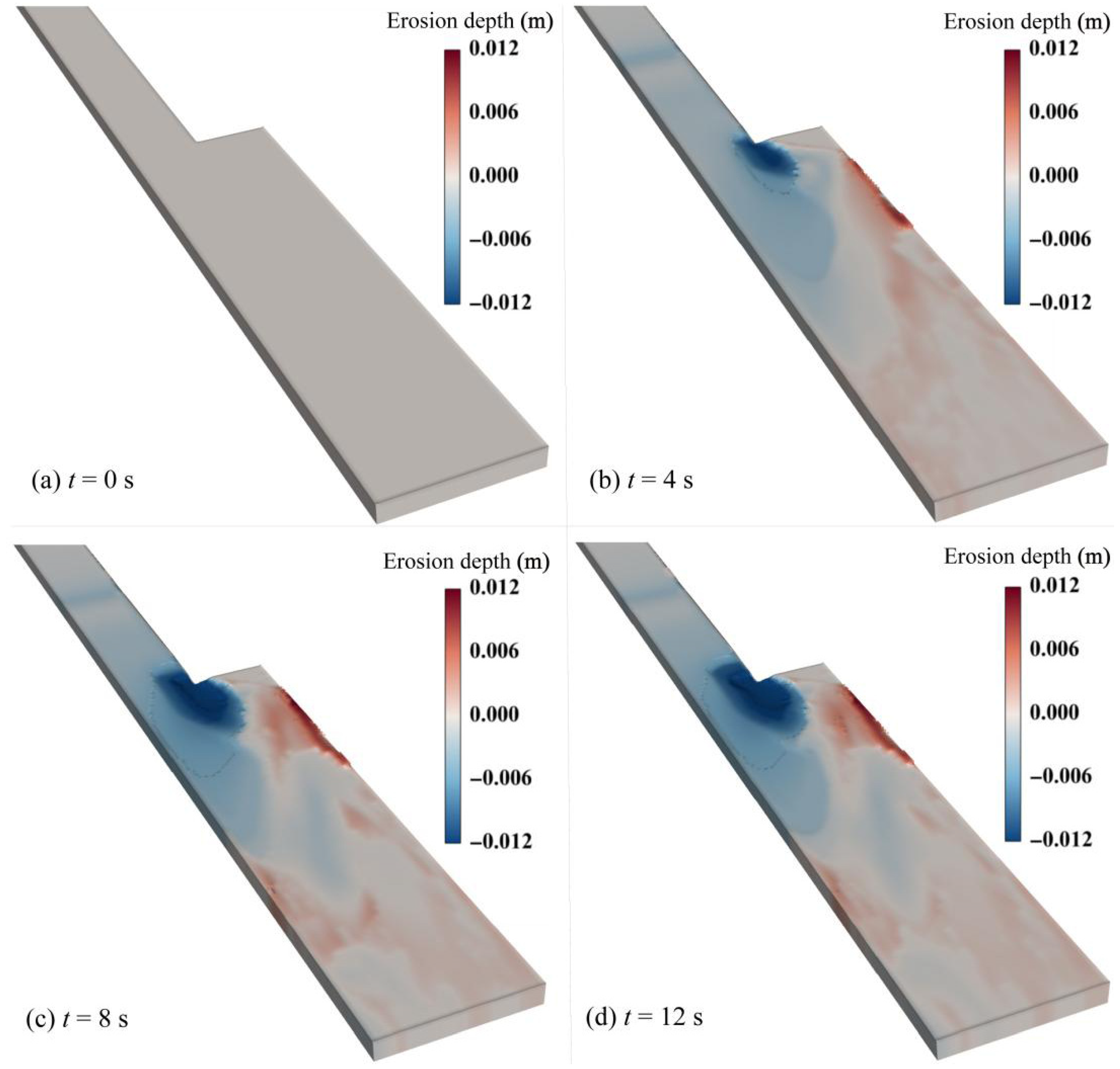
Figure 7 depicts the 3D calculation results of the sediment bed erosion depth at t = 0 s, 4 s, 8 s and 12 s. The blue regions are lower than the initial white bed surface, indicating sediment scouring and entrainment zones, while the red regions are higher than the initial white bed surface, representing sediment deposition zones. It can be clearly seen that the corner points in the sudden expansion region of the flume suffer the most severe scouring. Over time, the entrained sediment is transported by the flow and mostly deposits near the left sidewall of the downstream flume due to the obstruction of the solid boundary.

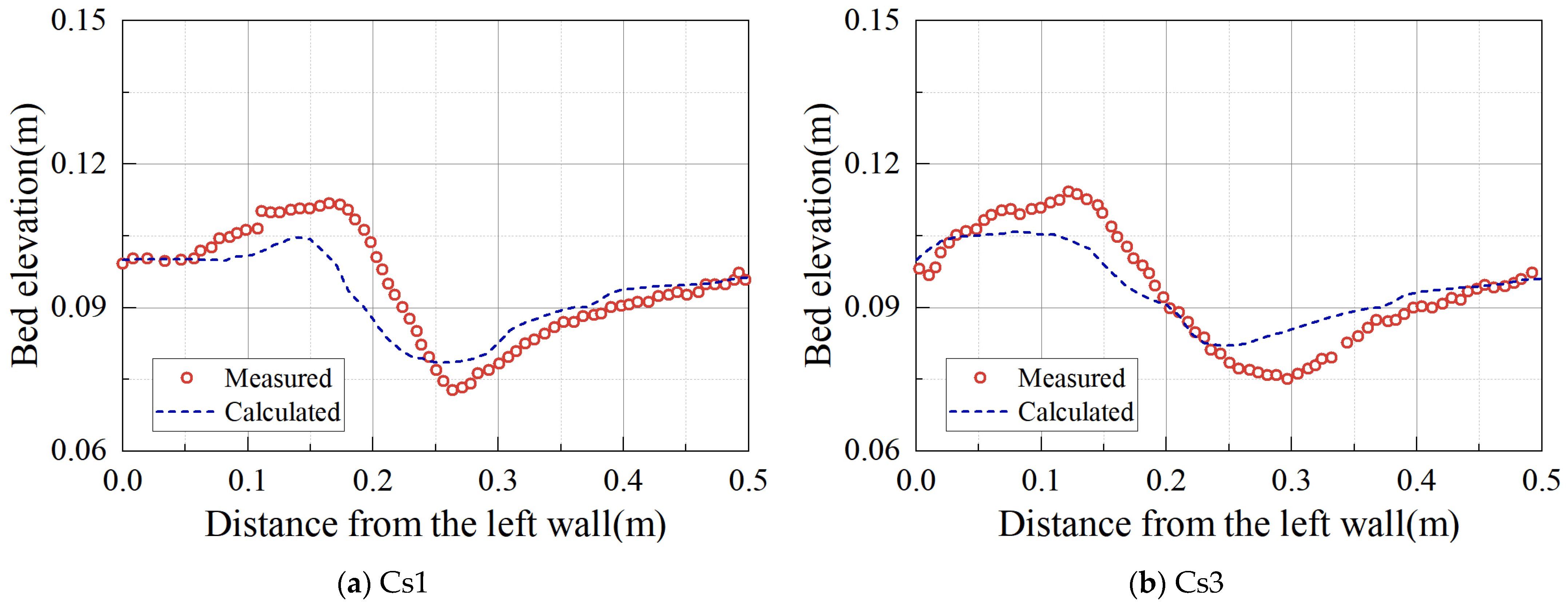
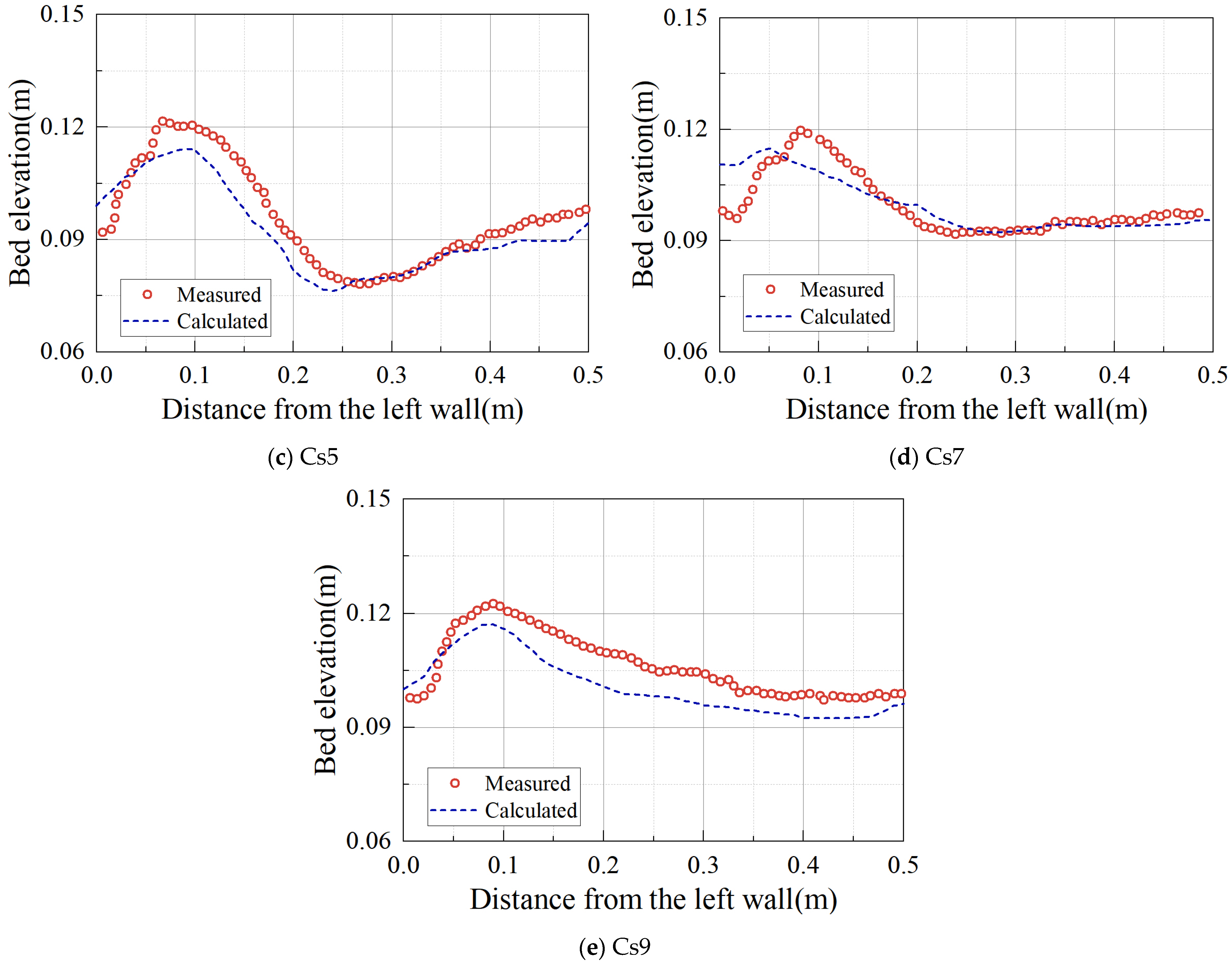
Typical cross-sections (Cs1, Cs3, Cs5, Cs7, and Cs9) were selected to calculate the bed elevation, which were compared with the measured bed profiles, as shown in Figure 8. To clarify the simulation accuracy of the erosion and accretion processes separately and avoid the defect of error offset between scouring and deposition zones, we conducted an independent statistical analysis for the scouring zone (bed elevation lower than the initial value) and deposition zone (bed elevation higher than the initial value) of the selected monitoring cross-sections.

Quantitative statistical results show that the average RMSE of bed elevation across all five monitoring cross-sections is 0.008 m, with the maximum RMSE of 0.011 m at cross-section Cs1 and the minimum RMSE of 0.005 m at cross-section Cs9. The overall NSE of bed elevation evolution reaches 0.88, and the overall PBIAS is −2.1%, indicating no significant overall overestimation or underestimation. For the scouring zone alone, the average RMSE of bed elevation is 0.009 m, with a maximum relative error of 11.2% and a PBIAS of −8.7%, which means slight underestimation of scouring depth. For the deposition zone alone, the average RMSE is 0.007 m, with a maximum relative error of 9.6% and a PBIAS of 6.3%, which means slight overestimation of deposition thickness. The errors of both the scouring zone and deposition zone are well within ±15%, and there is no significant offset between positive and negative errors. The global statistical results are highly consistent with the zone-separated statistical results, which fully proves that the numerical model can accurately capture the overall variation trend and spatiotemporal evolution law of the sediment bed elevation, exhibiting good consistency with the experimental measurements.

For the upstream cross-sections Cs1 and Cs3, the model slightly underestimates the maximum scouring depth in the middle region of the flume and the sediment deposition thickness near the left sidewall. For cross-sections Cs5, Cs7, and Cs9, the calculated bed elevation profiles are almost identical to the measured values. This minor local deviation is a common and acceptable phenomenon in similar numerical studies, and this is mainly because the actual sand bed in the flume test has natural spatial heterogeneity in particle gradation and compactness, which cannot be fully replicated by a single set of parameters. In addition, the flow at the sudden expansion corner has strong 3D turbulence, recirculation and small-scale vortex structures, and the turbulence model has inherent limitations in simulating such transient small-scale flow structures.

4. Validation Against Physical Dam Breach Flume Experiment

4.1. Two-Dimensional Dike Breach Case Study

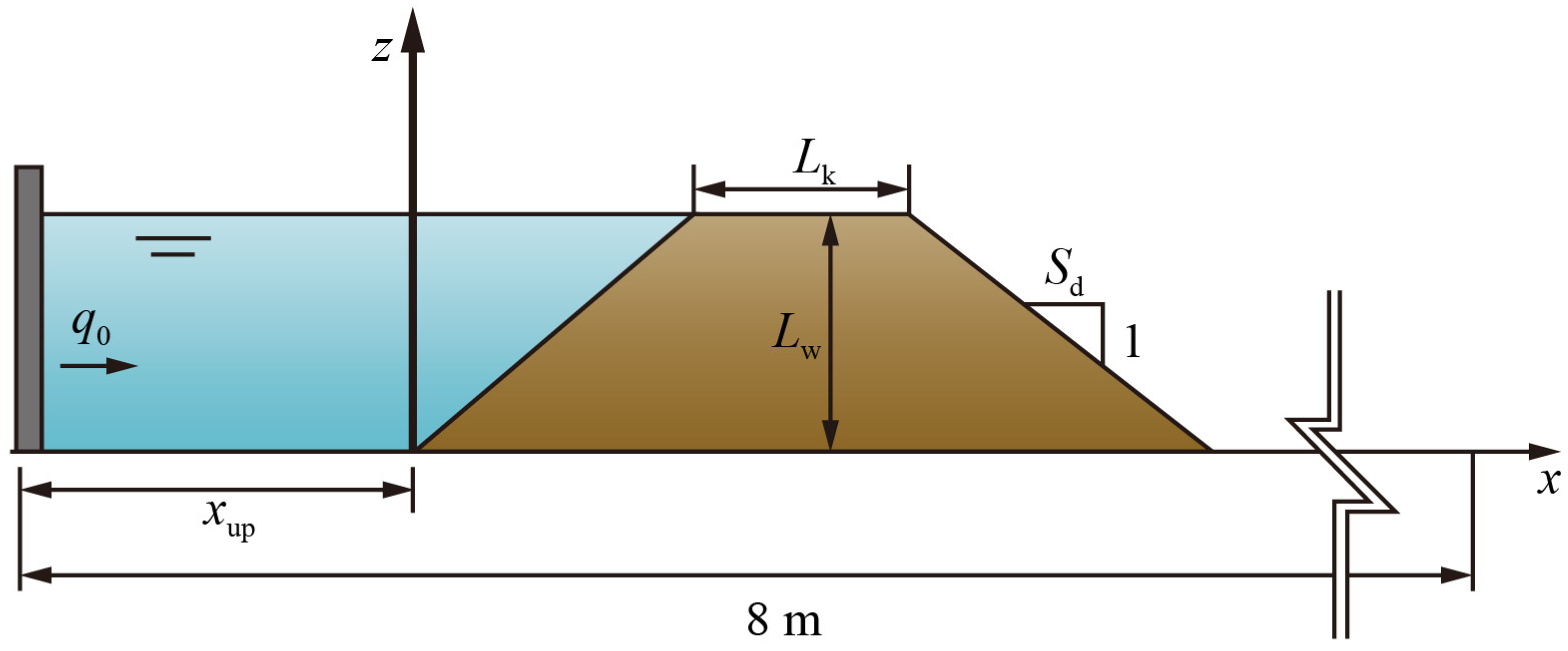
In this section, the two-dimensional dike breach experiment carried out by Schmocker is first selected as a case study [30] so as to validate the accuracy of the proposed numerical model in simulating the free surface and eroded bed profile. The layout condition of the numerical model is depicted in Figure 9. The upstream inflow q₀ = 0.006 m³/s, the distance from the upstream inflow section to the dam toe x_up = 1.0 m, the dam height L_w = 0.2 m, the crest length of the dike L_k = 0.1 m, the downstream slope ratio S_d = 2, and the median grain size of the dam material d₅₀ = 1.0 mm. The numerical model was discretized with a uniform structured grid, and grid sensitivity pre-analysis was conducted with three sets of grid resolutions (0.015 m, 0.02 m, and 0.025 m) to ensure the rationality of grid selection. The pre-simulation results indicate that the 0.02 m grid can accurately reproduce the evolution of the dam erosion profile and the dynamic change in the fluid free surface, and it significantly reduces the computational cost. Thus, a uniform grid with a 0.02 m resolution was adopted for this case, and the total computational duration was set to 20 s.

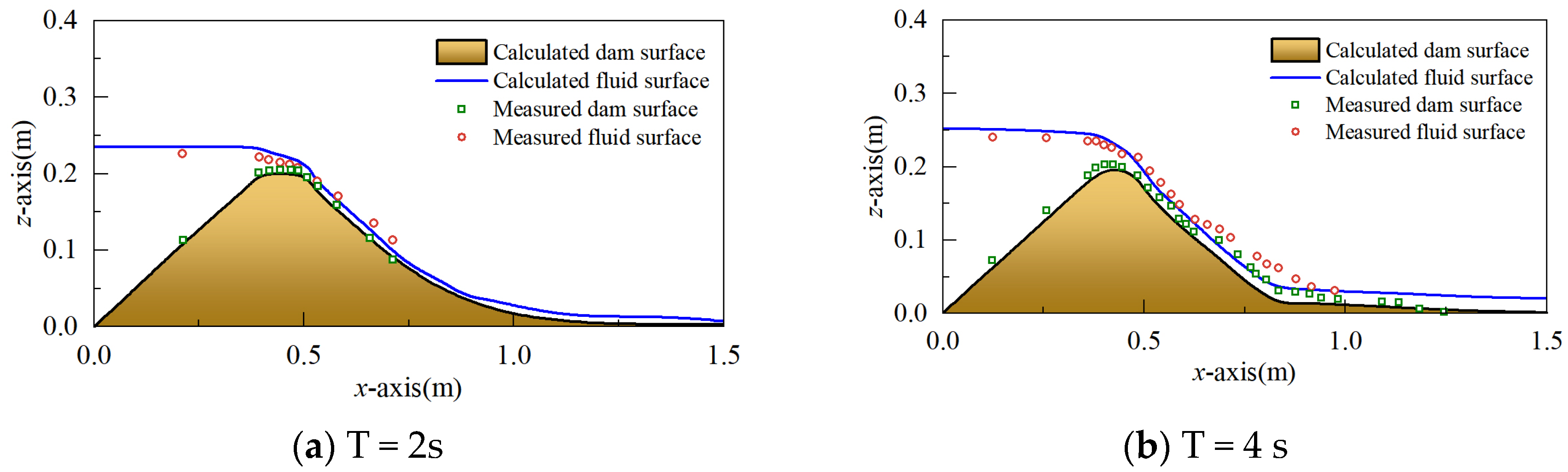
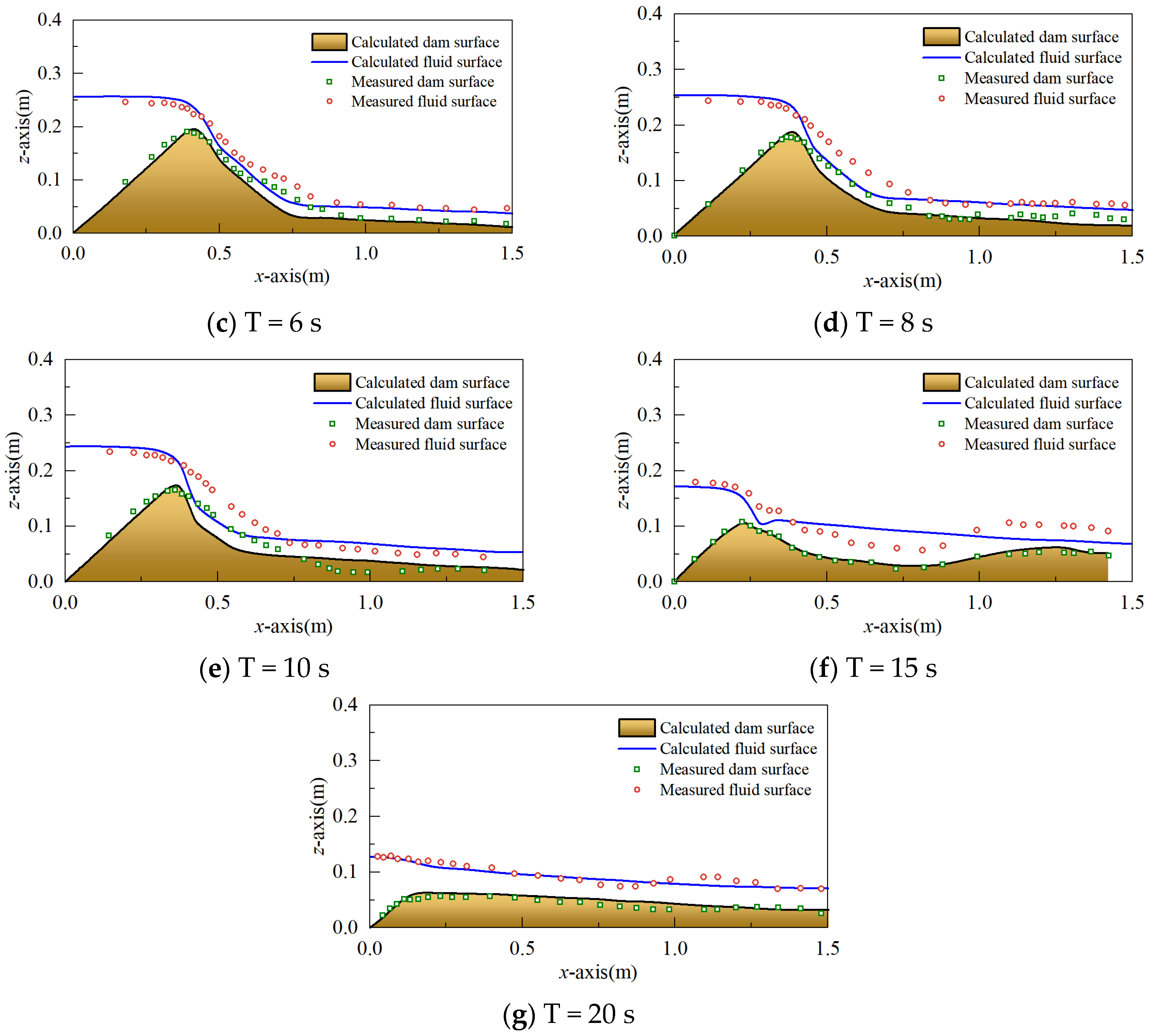
Figure 10 illustrates the temporal evolution of the calculated and measured dam and fluid free surfaces at seven key time instants during the 2D dike breach experiment. Across all time steps, the numerical model demonstrates remarkable consistency between calculated and measured results, which verifies the rationality of its case inversion. At the early stage (T = 2 s and T = 4 s), the calculated dam crest profile and fluid free surface align closely with the measured data, capturing the initial stability of the dam. As the breach progresses, the model effectively tracks the progressive erosion of the dam slope and the corresponding decline in fluid surface elevation, reproducing the dynamic breach process with high fidelity. For the key transient rapid incision stage of the breach (T = 10 s and T = 15 s), the independent quantitative error statistics show that at T = 10 s, the RMSE of the dam surface elevation is 0.022 m, with a relative error of 11.0%, and the RMSE of the fluid free surface elevation is 0.016 m, with a relative error of 7.8%. At T = 15 s, the RMSE of the dam surface elevation is 0.027 m, with a relative error of 13.5%, and the RMSE of the fluid free surface elevation of 0.019 m, with a relative error of 9.2%. The minor local discrepancy in the late stage of breach evolution is mainly caused by the fact that 3D numerical simulation cannot fully replicate the idealized plane strain condition of the 2D flume experiment.

By T = 20 s, the calculated residual dam profile and fluid surface are in excellent agreement with the measured results, confirming that the model can reliably simulate the entire evolution of the dike breach, from initial erosion to final equilibrium. The statistical results show that the average RMSE of the dam surface elevation across all time steps is 0.018 m, the average RMSE of the fluid free surface elevation is 0.011 m, the overall NSE of the dam surface elevation evolution reaches 0.91, and the relative error of the final residual dam crest elevation at 20 s is only 3.8%. Overall, the consistent alignment between numerical predictions and experimental observations validates the model’s ability to accurately replicate free surface dynamics and bed erosion characteristics.

4.2. General Description and Model Setup of Three-Dimensional Dam Breach Flume Experiment

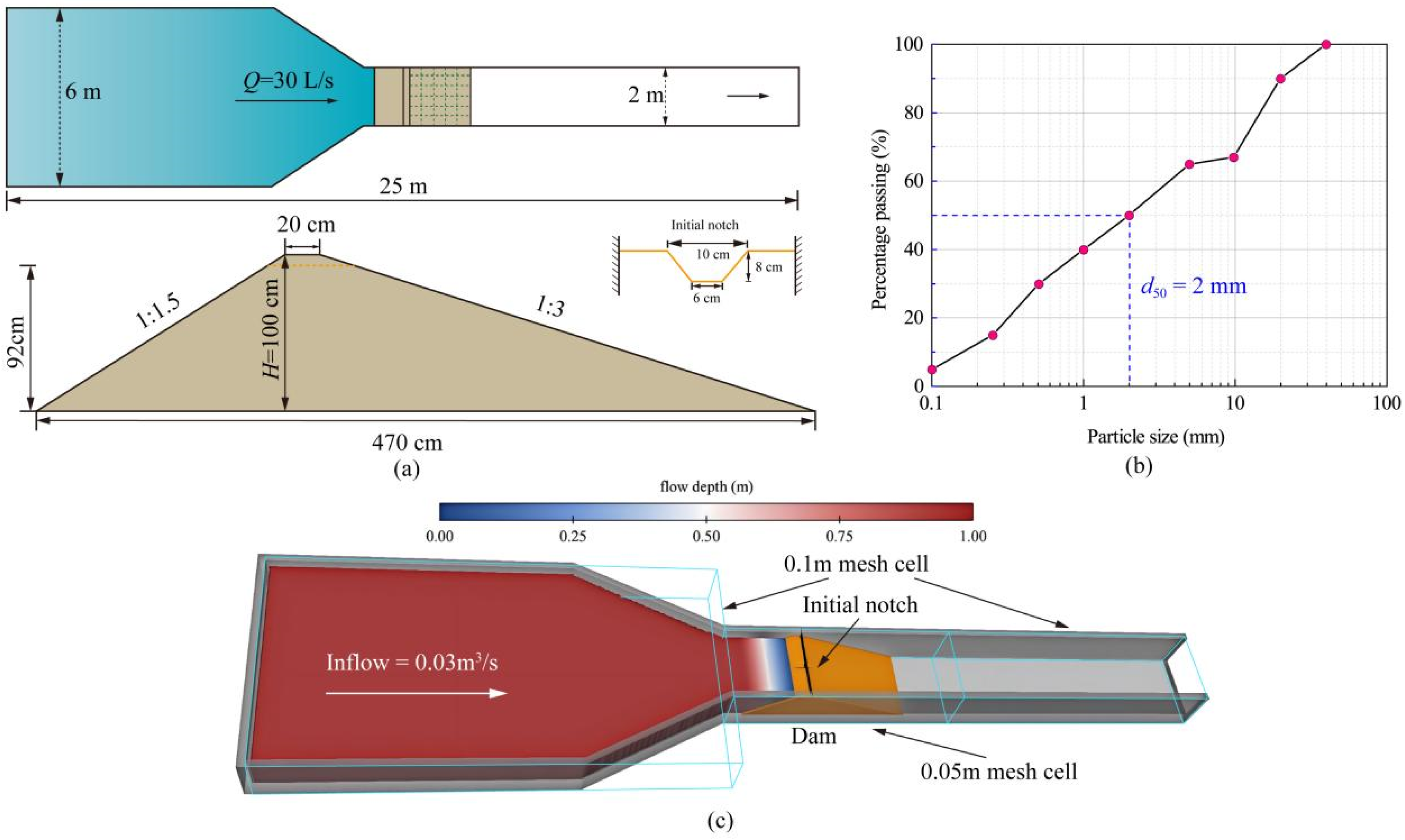
To further assess the practical accuracy of the proposed numerical model, a 3D flume test published by Duan et al. [31], which sufficiently replicates the entire breaching process of a non-cohesive earth dam, was adopted as a validation case. This experiment conducted detailed measurements of considerable breach-related data through high-resolution cameras, water level gauges, and other techniques, providing robust data support for in-depth analysis of the dam breach process. The experimental flume is configured with a length of 25 m and a height of 1.2 m. The upstream reservoir section has a width of 6 m, while the downstream weir section narrows to 2 m, with a maximum reservoir volume of approximately 80 m³. The longitudinal profile of the experimental dam model is presented in Figure 11a, which has a height of 100 cm, a crest width of 20 cm, and a base width of 470 cm. The slope ratios of the upstream and downstream slopes are 1:1.5 and 1:3 (V:H), respectively. A trapezoidal initial notch was excavated at the midpoint of the dam crest, with a bottom width of 6 cm and a depth of 8 cm. During the experiment, a constant inflow rate of Q = 30 L/s was supplied to the upstream reservoir. The model dam was constructed using non-cohesive discontinuous wide-graded gravel–sand geomaterials, with a particle size distribution ranging from 0.005 mm to 40 mm, which is shown in Figure 11b.

A rectangular computational domain was adopted for the numerical model, with length of 25 m, a width of 6 m, and a height of 1.5 m, as illustrated in Figure 11c. The initial water level was specified to coincide with the bottom elevation of the breach. The particle size distribution of the dam material adopted in the simulation is identical to that of the experimental model. The angle of repose is set at 38°, the entrainment coefficient is 0.018, and the bed load coefficient is 8. Within the computational domain, the top boundary is defined as a standard atmospheric pressure boundary, the upstream boundary is designated as a constant inflow boundary with a discharge of 0.03 m³/s, and the downstream boundary is specified as an outflow boundary. All remaining boundaries are configured as solid-wall no-slip boundaries. Furthermore, a discharge monitoring section is arranged at the breach to capture the temporal variation in breach discharge during the overtopping failure process. The total computational time is set to 400 s to satisfy the requirements of numerical validation.

4.3. Numerical Results

4.3.1. Sensitivity Analysis

To ensure the reliability of the numerical simulation results, eliminate systematic errors caused by grid discretization and erosion model selection, and further verify the robustness of the proposed model, two sets of systematic sensitivity analyses are conducted in this section, including grid convergence verification for spatial discretization and sensitivity analysis of erosion and sediment transport models for breach evolution simulation.

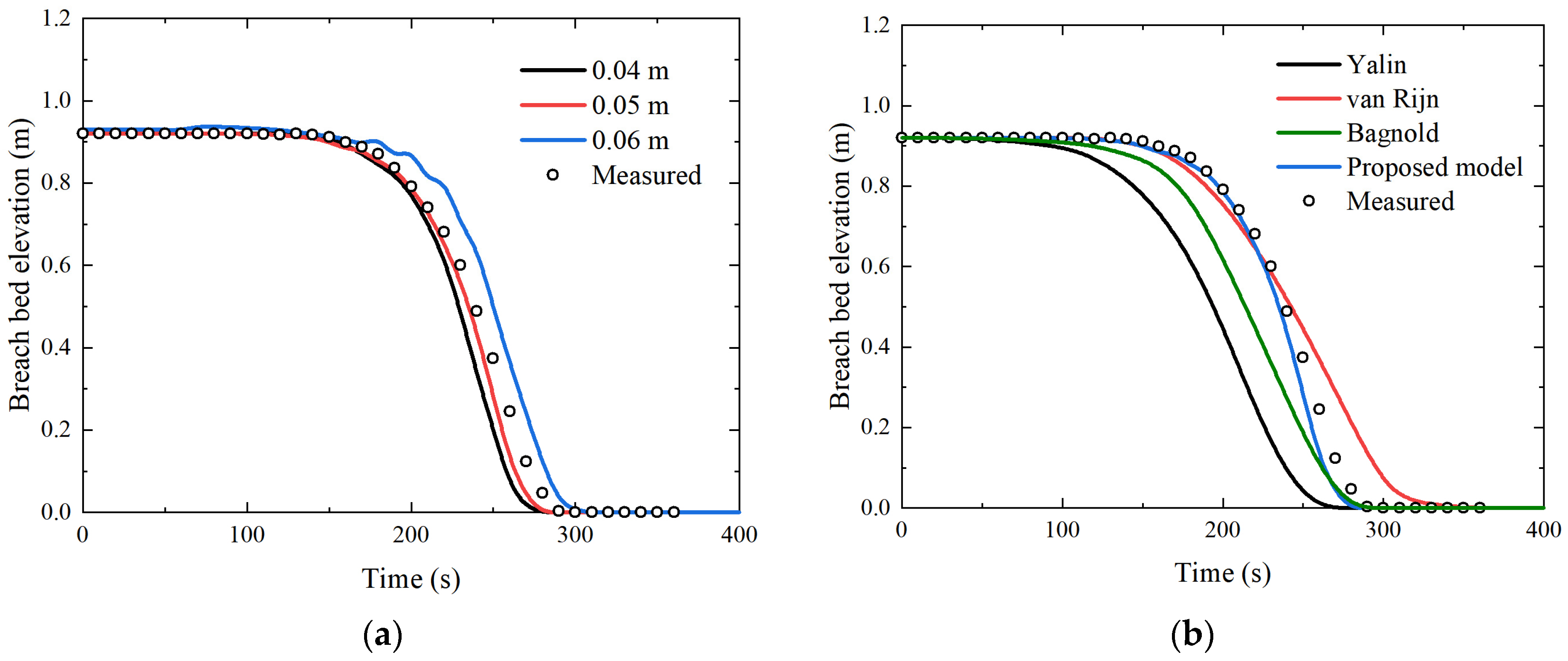
Given the well-documented sensitivity of dam breach simulations to near-wall grid resolution, a grid convergence verification was conducted to validate the reliability of the numerical results and justify the grid configuration adopted in this study. Three grid configurations were designed, featuring distinct global and refined domain resolutions to target the dynamically evolving breach zone: 0.12 m/0.06 m, 0.1 m/0.05 m and 0.08 m/0.04 m. The temporal evolution of the breach bed elevation under these configurations is compared with experimental measurements in Figure 12a. As illustrated in the figure, the grid resolution exerts a measurable influence on simulation accuracy. Coarser grids (0.12/0.06 m) show an obvious deviation from the measured data, with a significant underestimation of breach depth in the middle and later stages of dam failure. In contrast, the two refined grid configurations exhibit negligible differences in predicted erosion depth, accurately reproducing the temporal evolution of breach incision. Notably, in terms of computational efficiency, the 0.05 m refined grid shows a prominent advantage: it maintains the same level of simulation accuracy as the 0.04 m grid yet cuts the total computational time to only 45% of the latter, significantly reducing computational costs. Comprehensively balancing numerical precision, prediction stability and computational efficiency, the 0.10 m global grid with a 0.05 m refined grid in the breach zone is selected for all subsequent simulations, ensuring reliable high-fidelity results without excessive computational expense.

Furthermore, a sensitivity analysis of bedload erosion models was carried out to verify the rationality of the modified Meyer–Peter and Muller formula adopted in this study. Three classic and widely used bedload transport formulas for non-cohesive soils, including Yalin’s formula [32], van Rijn’s formula [33] and Bagnold’s formula [34], were selected for comparative simulation, with the measured breach bed elevation as the core evaluation indicator (see Figure 12b). The comparison results show that the Yalin formula significantly overestimates the vertical incision rate of the breach, while the Bagnold formula underestimates the erosion rate with a notable lag. The van Rijn formula shows a generally consistent trend with the measured value but still has phase deviation in the rapid incision stage. By comparison, the proposed model achieves optimal agreement with the measured data throughout the entire erosion process, with an RMSE of only 0.021 m, far lower than that of the Yalin formula (0.087 m), Bagnold formula (0.063 m) and van Rijn formula (0.038 m). This analysis fully proves the high accuracy and applicability of the proposed model.

4.3.2. Validation of Breach Hydrograph

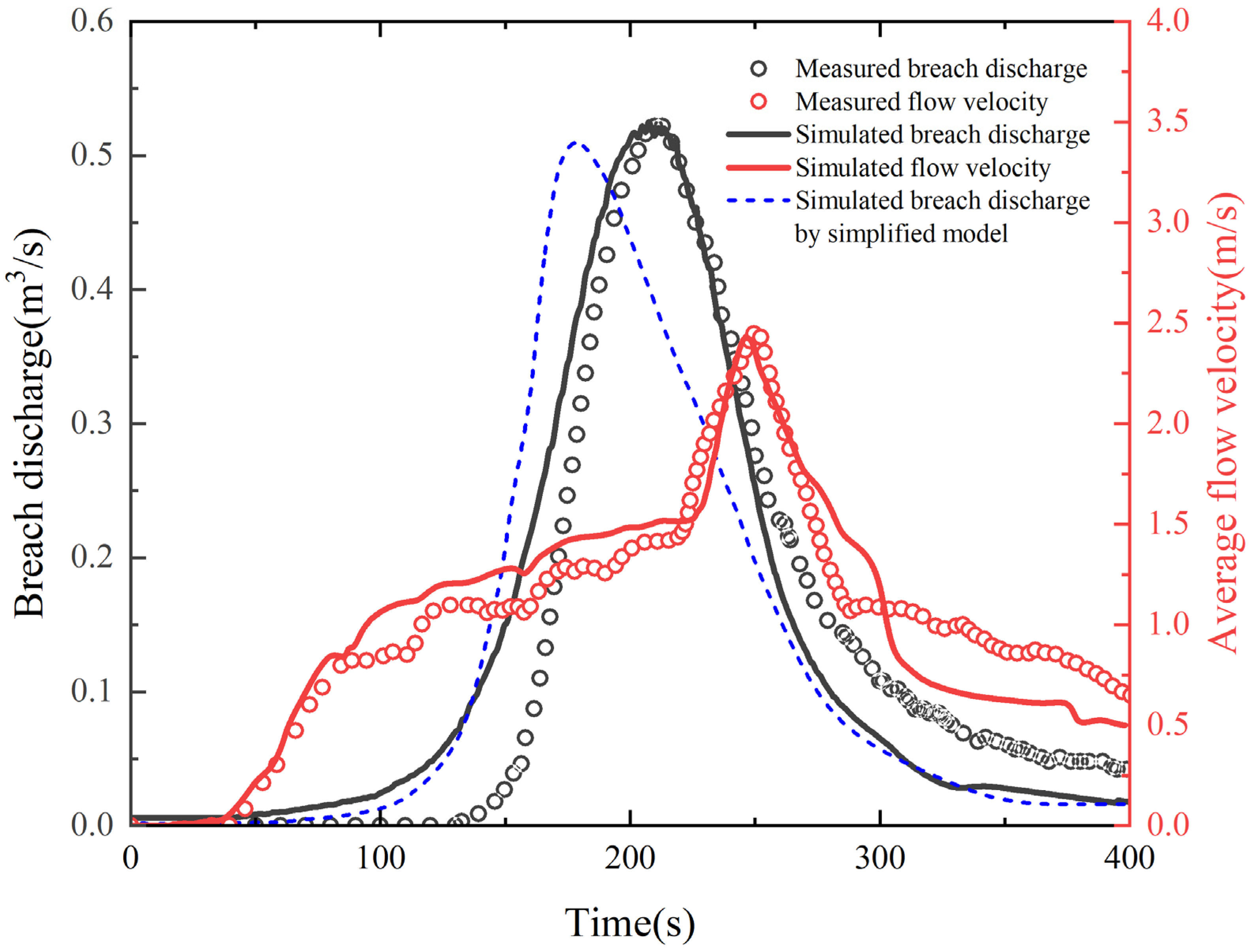
Figure 13 illustrates the temporal dynamics of the measured and simulated breach discharge and flow velocity during the breach process, synchronously characterizing the interconnected hydrodynamic parameters. To avoid the limitation of global time-series statistics, the whole breach process is divided into four stages for independent statistical analysis according to the breach evolution characteristics. In the initial phase (0~100 s), both measured data and simulated breach discharge remain near 0 m³/s, with limited water release. The RMSE of breach discharge is 0.008 m³/s, with a relative error less than 3%, and the simulated results accurately capture the initial stable state before full breach development. In the rapid rising stage (100~200 s), as the breach expands, the discharge surges sharply to a prominent peak. The RMSE of breach discharge is 0.032 m³/s, with a maximum point relative error of 12.6%. The local discrepancy in this stage is mainly caused by the extreme transient change in breach morphology and flow regime. In the peak and attenuation stage (200~300 s), the simulated peak breach discharge is 0.526 m³/s, while the measured value is 0.522 m³/s, with a relative error of only 0.77%. The RMSE of breach discharge in this stage is 0.027 m³/s, and the simulated curve closely matches the measured data in time to peak, magnitude, and subsequent attenuation trend. In the morphological stabilization stage (300~400 s), the breach discharge gradually stabilizes, with an RMSE of 0.011 m³/s and a relative error less than 4%.

The overall NSE of the breach discharge hydrograph reaches 0.94, and the overall PBIAS is 1.2%, indicating no significant overall overestimation or underestimation. To further verify the advancement of the proposed model, the mainstream DB-IWHR simplified dam breach model is selected for computation. The comparison results show that the peak breach discharge calculated by the DB-IWHR model is 0.492 m³/s, with a relative error of 5.74% compared with the measured data. Velocity remains negligible initially, surges sharply after 100 s, and then attenuates gradually. Furthermore, the numerically predicted breach velocity is 2.396 m/s, corresponding to a relative error of −2.08% compared to the measured value of 2.447 m/s. Overall, the comparison of two key breach characteristic parameters demonstrates that the proposed numerical results can well reflect the actual temporal evolution of breach discharge and velocity during the breach process.

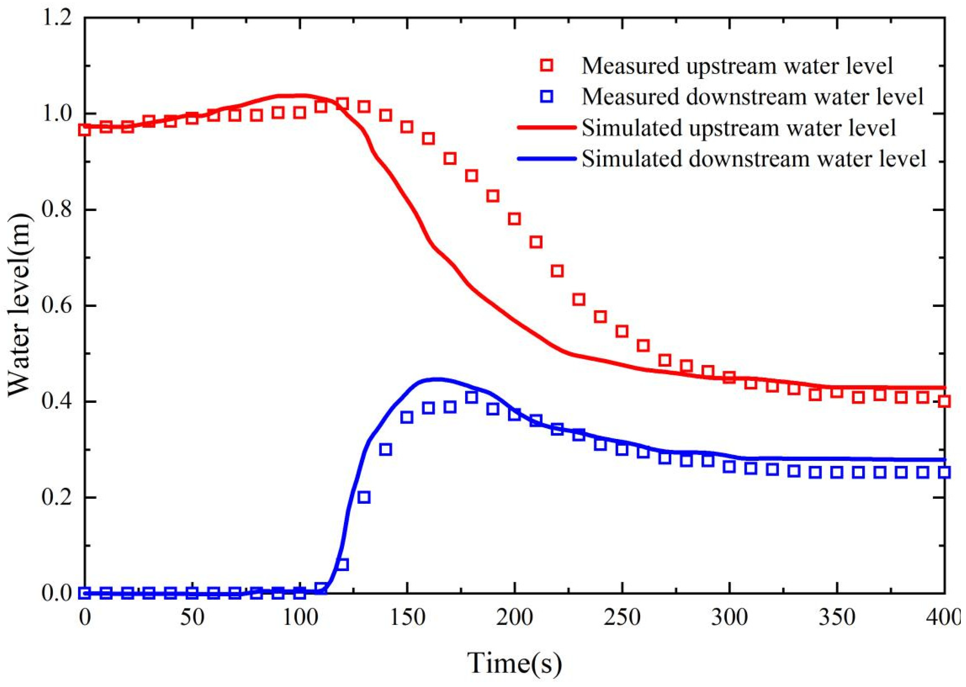
Figure 14 depicts the temporal evolution of the measured and simulated water levels both upstream and downstream of the breach throughout the dam breach process. For the upstream region, the simulated water level closely reproduces the initial stable stage and the rapid decline stage after breach initiation, with an RMSE of 0.021 m, a peak water level relative error less than 2.7%, and an overall NSE of 0.92. For the downstream region, the simulated results accurately capture the surge timing, peak magnitude, and rising rate of the flood wave, with an RMSE of 0.015 m, a flood wave arrival time relative error less than 3%, and an overall NSE of 0.89. The minor discrepancy in the water level decline stage is caused by the simplified treatment of the upstream inflow boundary in the numerical simulation, and the overall change trend and key characteristic values are in agreement with the experimental measurements.

4.3.3. Validation of Breach Evolution

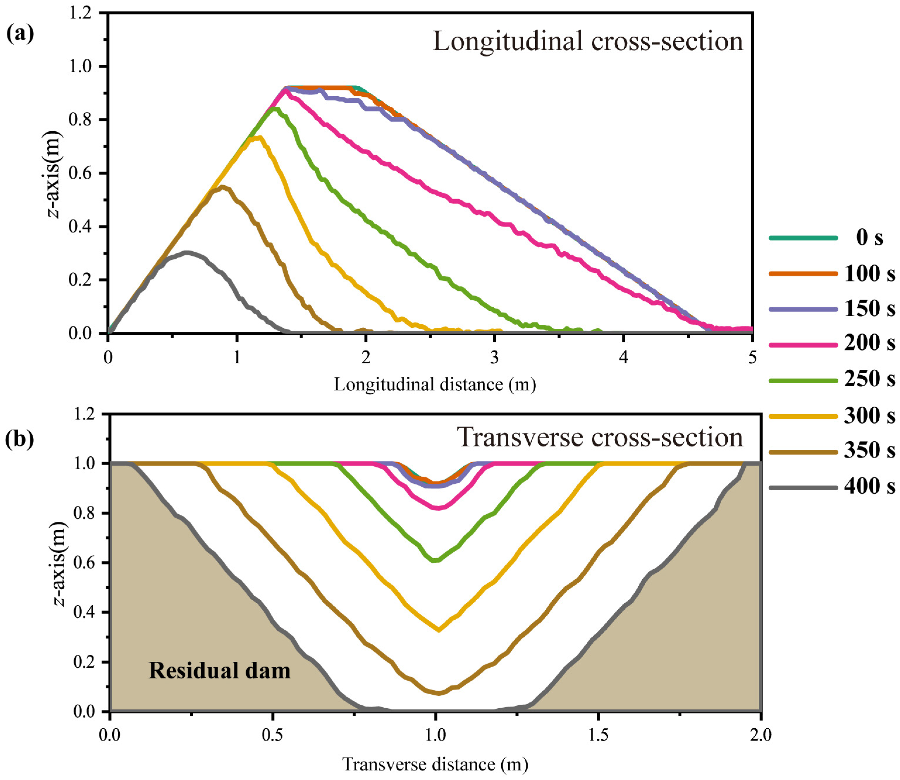
Figure 15 indicates the simulated spatiotemporal evolution of breach morphology across the longitudinal (a) and transverse (b) cross-sections at different time intervals during the dam breach process. At 0 s, the longitudinal profile presents an intact trapezoidal dam structure, consistent with the initial configuration of the flume model, and the transverse profile is a flat, intact dam crest. Within the first 100s, the breach is dominated by surface erosion in the longitudinal section, with minimal changes in the dam body relative to the initial state. This stage coincides with the low-discharge regime (Figure 13) and upstream water level retention period (Figure 14) prior to full breach activation.

As time progresses, continuous erosion of the dam crest and downstream slope gradually flattens the longitudinal profile, leading to a reduction in crest elevation and a decrease in downstream slope angle. This pattern is consistent with the breach evolution law proposed by conventional simplified dam breach models [14]. The sequential profiles clearly reveal the unsteady longitudinal expansion characteristics of the breach: the eroded area extends along the flume length, while the residual elevation decreases continuously. Subsequently, at around 150 s (synchronized with the peak discharge phase in Figure 13), the breach rapidly incises and expands under the alternating effects of sediment entrainment and slope instability. The transverse profiles indicate that the concave region expands continuously, while the sidewall slopes connecting the breach to the residual dam body gradually become gentler. This lateral expansion phenomenon fully demonstrates the analytical capacity of the breach development module (incorporating sediment transport and instability mechanisms) in resolving the dynamic expansion process of the breach for the non-cohesive dam, which is often oversimplified in most existing dam breach models. To further verify the model’s accuracy in simulating breach geometry evolution, we compared the simulated final stable breach dimensions with the flume experimental measurements. The simulated final breach depth and top width are 0.84 m and 1.82 m, respectively, which are in good agreement with the experimental measured values of 0.82 m and 1.76 m.

4.3.4. Simulation and Observation of Dam Breach Process

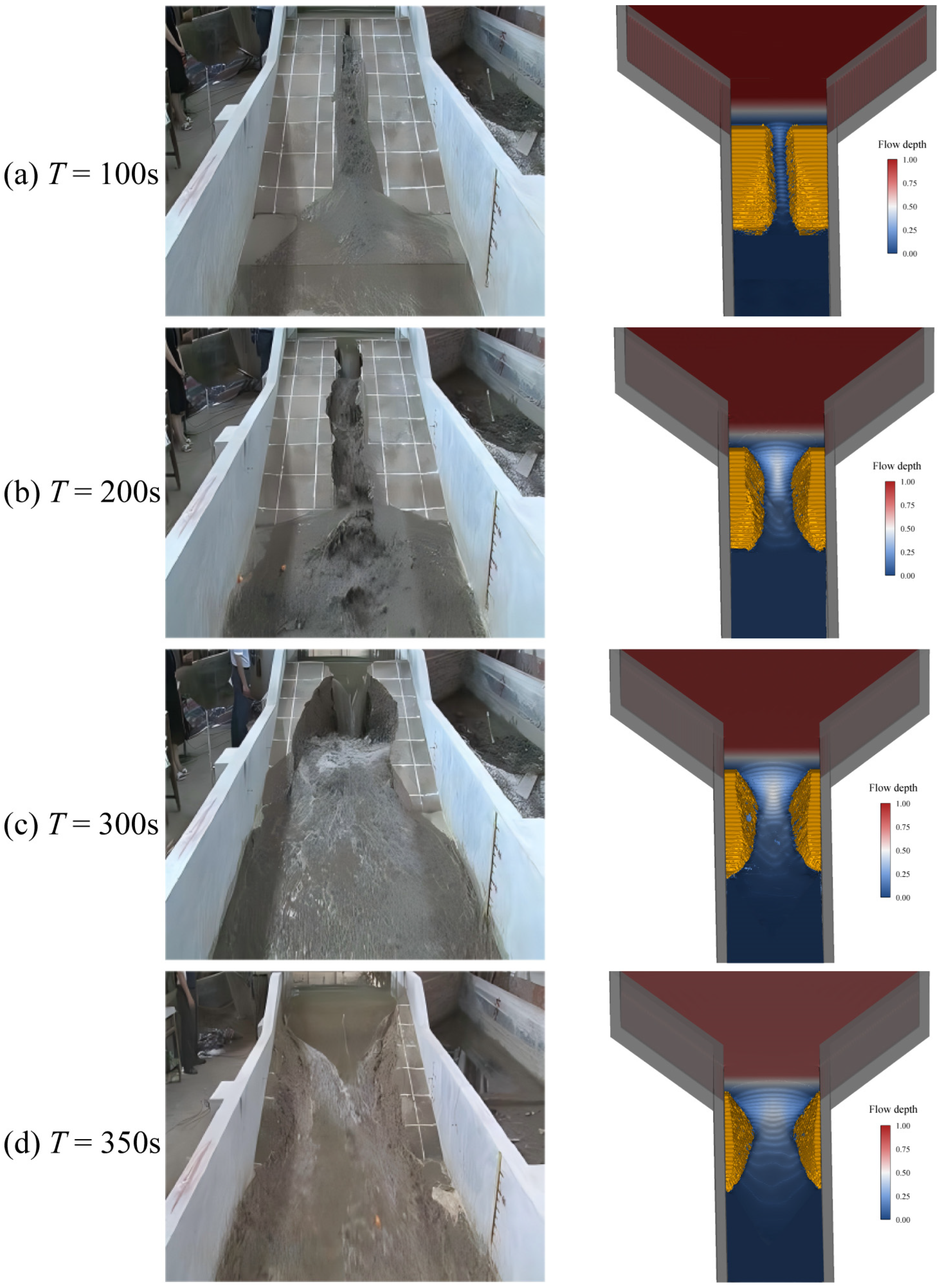
Figure 16 compares the experimental visualization and numerical simulation results of the three-dimensional overtopping-induced breach process at different stages. Based on the breach discharge dynamics and morphological evolution characteristics, the breach process can be divided into four sequential phases: surface erosion, retrogressive erosion, rapid erosion, and morphological stabilization.

Surface erosion phase (0~100 s): Overtopping flow initiates from the dam crest and accelerates along the downstream slope, gradually enhancing erosivity to form rill-like surface erosion. This phase is dominated by gradual erosion on the downstream slope, and breach discharge and velocity remain low, while the upstream reservoir water level rises slowly.

Retrogressive erosion phase (100~200 s): Driven by flow erosion and sediment transport, the rill incises longitudinally and widens transversely via lateral scouring and gravity-induced bank collapse, while the sediment carried by slope flow deposits in a fan shape around the rill outlet at the downstream slope toe. Erosion remains concentrated on the downstream slope, with gradually increasing overtopping flow erosivity. Breach discharge and velocity rise slowly, and the upstream reservoir water level starts to decrease after reaching its peak.

Rapid erosion phase (200~300 s): This phase is characterized by intense dam collapse, with the strongest flow magnitude. The breach retreats upstream continuously, and the peak breach discharge and velocity occur in this stage, while the upstream reservoir drops sharply.

Morphological stabilization phase (300~400 s): The erosivity of breach flow gradually weakens, and the dam erosion process slows down until stabilization. The breach outflow reaches a dynamic balance with the upstream inflow, marking the end of the dam breach process.

5. Conclusions

This study develops an improved 3D detailed numerical model for simulating the overtopping-induced breach process and morphological evolution of non-cohesive earth dams. The proposed model integrates three core modules with two-way coupling between flow and topographic changes. The RNG k-ε turbulence model and VOF method effectively capture the 3D flow field and free surface dynamics during overtopping, while the modified sediment erosion formula accounts for the effects of particle gradation on erosion. Moreover, the breach development module, which combines erosion and gravitational collapse, successfully reproduces the vertical deepening and lateral widening of non-cohesive dam breaches.

Systematic validations are conducted through a classic movable-bed dam break benchmark case and a full-scale flume experiment of non-cohesive earth dam overtopping failure. Multi-dimensional statistical results show that the model can accurately reproduce the full evolutionary process of the dam breach, with the relative errors of key parameters, including peak breach discharge, time to peak, final breach depth and top width, all controlled within 5%. The overall NSE of the breach hydrograph, water level change and bed elevation evolution is greater than 0.85, and the maximum point error in the transient rapid erosion stage is within ±15%. The model reliably captures the synchronous vertical deepening and lateral widening of the breach, providing a high-fidelity numerical tool for the detailed simulation of non-cohesive earth dam overtopping failure.

Despite the reliable overall performance, the study has several objective limitations that may lead to minor local deviations in simulation results. The current model adopts sediment parameters with different particle gradation across the entire computational domain, which cannot fully replicate the natural spatial heterogeneity of compactness in actual dam materials. The slope stability criterion is simplified based on the angle of repose for fully saturated non-cohesive soils, without considering the effects of transient pore water pressure and soil cohesion, which restricts the model’s direct application to cohesive or partially saturated earth dams. In addition, this study focuses on the validation of the fully coupled model and has not yet conducted independent rigorous testing of each individual module and the error transmission between coupled modules.

Future research will focus on addressing these limitations to further improve the model’s reliability and expand its engineering applicability. Rigorous module-wise benchmark testing will be carried out to verify the performance of the hydrodynamic, erosion and breach development modules independently and to quantify the error transmission law during the multi-physics coupling process. Comprehensive comparative tests of classic bedload transport formulas and global sensitivity analysis of core parameters will be conducted to optimize the model’s calibration method and clarify the influence of formula and parameter selection on simulation results. The slope stability criterion will be refined by introducing cohesive parameters and transient pore water pressure calculation to extend the model’s applicability to cohesive and wide-graded earth dams. The sub-time-step coupling algorithm will also be optimized to enhance the temporal consistency and numerical stability of the model to better support dam breach risk assessment, emergency management and engineering design in practical projects.

References

1. Sadeghi, S.; Hakimzadeh, H.; Amini, A. Experimental investigation into outflow hydrographs of nonhomogeneous earth dam breaching due to overtopping. J. Hydraul. Eng. 2020, 146, 04019049. [Google Scholar] [CrossRef]
2. Shen, D.; Shi, Z.; Peng, M.; Zhang, L.; Jiang, M. Longevity analysis of landslide dams. Landslides 2020, 17, 1797–1821. [Google Scholar] [CrossRef]
3. Cai, Y.; Cheng, H.; Wu, S.; Yang, Q.; Wang, L.; Luan, Y.; Chen, Z. Breaches of the Baige barrier lake: Emergency response and dam breach flood. Sci. China Technol. Sci. 2020, 63, 1164–1176. [Google Scholar] [CrossRef]
4. Zhong, Q.; Wang, L.; Chen, S.; Chen, Z.; Shan, Y.; Zhang, Q.; Ren, Q.; Mei, S.; Jiang, J.; Hu, L.; et al. Breaches of embankment and landslide dams—State of the art review. Earth-Sci. Rev. 2021, 17, 2931–2956. [Google Scholar] [CrossRef]
5. Aureli, F.; Maranzoni, A.; Petaccia, G. Advances in Dam-Break Modeling for Flood Hazard Mitigation: Theory, Numerical Models, and Applications in Hydraulic Engineering. Water 2024, 16, 1093. [Google Scholar] [CrossRef]
6. Yang, P.; Xu, F.; Ye, X.; Li, F.; Xu, X.; Wu, Y.; Ouyang, L. Experimental Study on the Mechanism of Overtopping Failure and Breach Development in Homogeneous Earth Dams. Water 2025, 17, 3352. [Google Scholar] [CrossRef]
7. Zhang, J.; Yang, X.; Fan, G.; Li, H.; Zhou, J. Physical and numerical modeling of a landslide dam breach and flood routing process. J. Hydrol. 2024, 628, 130552. [Google Scholar] [CrossRef]
8. ASCE/EWRI Task Committee on Dam/Levee Breaching. Earthen embankment breaching. J. Hydraul. Eng. 2011, 137, 1549–1564. [Google Scholar] [CrossRef]
9. Froehich, D. Embankment dam parameters and their uncertainties. J. Hydraul. Eng. 2008, 134, 1708–1721. [Google Scholar] [CrossRef]
10. Peng, M.; Zhang, L. Breaching parameters of landslide dams. Landslides 2012, 9, 13–31. [Google Scholar] [CrossRef]
11. Azmi, M.; Thomson, K. Dam breach parameters: From data-driven-based estimates to 2-dimensional modeling. Nat. Hazards 2024, 120, 4423–4461. [Google Scholar] [CrossRef]
12. Wu, W. Simplified physically based model of earthen embankment breaching. J. Hydraul. Eng. 2013, 139, 837–851. [Google Scholar] [CrossRef]
13. Ma, J.; Zhou, F.; Yue, C.; Sun, Q.; Wang, X. The Coupled Application of the DB-IWHR Model and the MIKE 21 Model for the Assessment of Dam Failure Risk. Water 2024, 16, 2919. [Google Scholar] [CrossRef]
14. Zhong, Q.; Chen, S.; Deng, Z. Numerical model for homogeneous cohesive dam breaching due to overtopping failure. J. Mt. Sci. 2017, 14, 571–580. [Google Scholar] [CrossRef]
15. Macchione, F.; Lorenzo, G.; Graziano, A. Study of key aspects in simplified modelling of man-made earthen dams breaching: Breach shape, erosion process and hydraulics. J. Hydrol. 2023, 620, 129425. [Google Scholar] [CrossRef]
16. Paul, M.; Julien, P. Test and improvement of 1D routing algorithms for dam-break floods. J. Hydraul. Eng. 2020, 146, 04020043. [Google Scholar] [CrossRef]
17. Dazzi, S.; Vacondio, R.; Mignosa, P. Integration of a levee breach erosion model in a GPU-accelerated 2D shallow water equations code. Water Resour. Res. 2019, 55, 682–702. [Google Scholar] [CrossRef]
18. Guan, M.; Wright, N.; Sleigh, P. 2D process-based morpho-dynamic model for flooding by non-cohesive dyke breach. J. Hydraul. Eng. 2014, 140, 04014022. [Google Scholar] [CrossRef]
19. Mei, S.; Chen, S.; Zhong, Q.; Shan, Y. Detailed numerical modeling for breach hydrograph and morphology evolution during landslide dam breaching. Landslides 2022, 19, 2925–2949. [Google Scholar] [CrossRef]
20. Peziale, C.; Sarkar, S.; Gatski, T. Modelling the pressure-strain correlation of turbulence: An invariant dynamical systems approach. J. Fluid Mech. 1991, 227, 245–272. [Google Scholar] [CrossRef]
21. Hirt, C.; Nichols, B. Volume of fluid (VOF) method for the dynamics of free boundaries. J. Comput. Phys. 1981, 39, 201–225. [Google Scholar] [CrossRef]
22. Yakhot, V.; Orszag, S.; Thangam, S.; Gatski, T.; Speziale, C. Development of turbulence models for shear flows by a double expansion technique. Phys. Fluids A Fluid Dyn. 1992, 4, 1510–1520. [Google Scholar] [CrossRef]
23. Mastbergen, D.; van den Berg, J. Breaching in fine sands and the generation of sustained turbidity currents in submarine canyons. Sedimentology 2003, 50, 625–637. [Google Scholar] [CrossRef]
24. van Rijn, L. Erodibility of mud-sand bed mixtures. J. Hydraul. Eng. 2020, 146, 04019050. [Google Scholar] [CrossRef]
25. Roseberry, J.; Schmeeckle, M.; Furbish, D. A probabilistic description of the bed load sediment flux: 2. particle activity and motions. J. Geophys. Res. Earth Surf. 2012, 117, F03032. [Google Scholar] [CrossRef]
26. Meyer-Peter, E.; Muller, R. Formulas for bed load transport. Process Congr. IAHR 1948, 6, 39–64. [Google Scholar]
27. Samma, H.; Khosrojerdi, A.; Rostam-Abadi, M.; Mehraein, M.; Cataño-Lopera, Y. Numerical simulation of scour and flow field over movable bed induced by a submerged wall jet. J. Hydroinform. 2020, 22, 385–401. [Google Scholar] [CrossRef]
28. Choufu, L.; Abbasi, S.; Pourshahbaz, H.; Taghvaei, P.; Tfwala, S. Investigation of Flow, Erosion, and Sedimentation Pattern around Varied Groynes under Different Hydraulic and Geometric Conditions: A Numerical Study. Water 2019, 11, 235. [Google Scholar] [CrossRef]
29. Goutiere, L.; Soares-Frazao, S.; Zech, Y. Dam-break flow on mobile bed in abruptly widening channel: Experimental data. J. Hydraul. Res. 2011, 49, 367–371. [Google Scholar] [CrossRef]
30. Schmocker, L. Hydraulics of Dike Breaching; Mitteilungen 218; Versuchsanstalt für Wasserbau, Hydrologie und Glaziologie (VAW): Zürich, Switzerland, 2011. [Google Scholar]
31. Duan, W.; Yang, W.; Wang, S.; Li, L. Overtopping failure process of cohesionless earth dam. J. Yangtze River Sci. Res. Inst. 2012, 29, 68–72. [Google Scholar] [CrossRef]
32. Yalin, M. An expression for bed-load transportion. J. Hydraul. Div. 1963, 89, 221–250. [Google Scholar] [CrossRef]
33. van Rijn, L. Sediment transport, Part I: Bed load transport. J. Hydraul. Eng. 1984, 110, 1431–1456. [Google Scholar] [CrossRef]
34. Bagnold, R. An Approach to the Sediment Transport Problem from General Physics; U.S. Geological Survey Professional Paper; U.S. Government Printing Office: Washington, DC, USA, 1966; Volume 422, pp. 231–291.
Figure 1. Schematic diagram of the dam material erosion module.
Water 18 00880 g001
Figure 2. Schematic diagram of bed level updating of two adjacent computational cells.
Water 18 00880 g002
Figure 3. Calculation flow chart of the proposed numerical model.
Water 18 00880 g003
Figure 4. Layout schematic of the sudden-expansion open-channel dam break test. The positions of the 8 water level monitoring points (P1~P8) for flow depth measurement and 9 bed elevation monitoring cross-sections (Cs1~Cs9) for scouring and deposition observation are marked in the figure.
Water 18 00880 g004
Figure 5. Calculated flow depth contour maps at various time intervals.
Water 18 00880 g005
Figure 6. Comparison of the measured and calculated water levels at each monitoring point.
Water 18 00880 g006
Figure 7. The three-dimensional calculated results of soil erosion depths at various time intervals.
Water 18 00880 g007
Figure 8. Comparison of the measured and calculated bed profiles at different cross-sections.
Water 18 00880 g008aWater 18 00880 g008b
Figure 9. Schematic diagram of the experimental setup for the 2D dike breach test.
Water 18 00880 g009
Figure 10. Comparison of the measured and calculated dam and fluid free surfaces at different times.
Water 18 00880 g010aWater 18 00880 g010b
Figure 11. Model setup of the flume experiment: (a) sketch of the experimental flume and model dam; (b) grain size distribution curve of dam material in the test; (c) setup of the numerical simulation.
Water 18 00880 g011
Figure 12. Sensitivity analysis results: (a) temporal evolution of breach bed elevation under different grid configurations; (b) performance comparison of different bedload erosion models against experimental measurements.
Water 18 00880 g012
Figure 13. Measured and simulated temporal dynamics of breach discharge and flow velocity compared with the results of the simplified model.
Water 18 00880 g013
Figure 14. Temporal evolution of measured and simulated upstream and downstream water levels during the breach process.
Water 18 00880 g014
Figure 15. Breach morphology evolution: (a) simulated breach longitudinal profile; (b) simulated breach transverse profile.
Water 18 00880 g015
Figure 16. Measured and simulated three-dimensional overtopping-induced breach processes.
Water 18 00880 g016