Article

Dam Deformation Prediction Based on MHA-BiGRU Framework Enhanced by CEEMD–iForest Outlier Detection


1
Guangxi Guiguan Electric Power Co., Ltd., Nanning 530000, China
2
Large Dam Safety Supervision Center, National Energy Administration, Hangzhou 310014, China
3
College of Water Conservancy and Hydropower Engineering, Hohai University, Nanjing 210098, China
4
The National Key Laboratory of Water Disaster Prevention, Hohai University, Nanjing 210098, China
5
National Engineering Research Center of Water Resources Efficient Utilization and Engineering Safety, Hohai University, Nanjing 210098, China
6
Institute of Water Science and Technology, Nanjing 210098, China
*
Author to whom correspondence should be addressed.
Water 2026, 18(4), 516; https://doi.org/10.3390/w18040516
Submission received: 24 January 2026 / Revised: 6 February 2026 / Accepted: 8 February 2026 / Published: 21 February 2026

Abstract

Notably, one of the key points to address low accuracy and delayed responsiveness of dam deformation prediction models lies in the timely detection of the outliers caused by environmental disturbances, sensor failures, or operational anomalies of dam monitoring sequences. Therefore, our work offers an unambiguous method for overcoming this challenge. In this paper, a robust prediction framework that integrates Complete Ensemble Empirical Mode Decomposition (CEEMD) and Isolation Forest (iForest) for effective outlier detection, followed by a Multi-Head Attention Bidirectional Gated Recurrent Unit (MHA-BiGRU) model for dam deformation prediction, is presented. The original deformation time series is first decomposed using CEEMD into a set of intrinsic mode functions (IMFs). This decomposition separates the series into trend-related components and noise components. Subsequently, the iForest algorithm is applied in outlier detection for noise components. Then, the BiGRU model is enhanced with an MHA mechanism to give more weight to the features that affect the sequences of monitoring dam deformation. By enabling the proposed model to focus on the key factors affecting dam deformation, the accuracy of the prediction results has been enhanced. Finally, a case study introducing monitoring data from a practical project in China demonstrates the performance of the proposed method. The proposed MHA-BiGRU model demonstrates superior performance across all tested scenarios. Notably, the coefficient of determination is consistently maintained above 0.98, peaking at 0.9880. In terms of error control, the model exhibits a maximum mean absolute error of 0.1789, thereby substantiating its exceptional prediction accuracy and robustness. In comparison with classical time series forecasting models, including LSTM, GRU and BiGRU, the proposed approach demonstrates enhanced robustness and delivers greater prediction accuracy. The findings provide a promising reference framework for dam structural characteristics prediction in similar projects.

1. Introduction

Dams play a crucial regulatory role in hydrological, ecological, and socioeconomic systems. The reliable use case of dams is a vital factor for flood control, drought mitigation, water supply stabilization, hydropower optimization, and ecological flow maintenance [1,2,3]. Ensuring the safe lifetime of a dam is essential for optimizing hydraulic engineering operations and fully exploiting their regulation potential under complex hydrometeorological conditions [4,5,6]. Globally, many regions have experienced dam failures caused by abnormal deformation, directly resulting in severe economic losses and losses of human lives. Previous studies have revealed that dam deformation serves as the most intuitive indicator for assessing dam structural safety; it is essential to monitor such changes in a timely manner and implement appropriate countermeasures accordingly [7,8,9]. Therefore, forecasting for dam deformation has emerged as a central task in dam safety control, and accurate forecasting leads to stable and long-term operation of dams [10].
However, due to factors such as the observation environment, transmission links, and monitoring equipment malfunctions, dam deformation monitoring sequences are often contaminated by outliers [11,12]. Without proper detection and treatment, these outliers can hinder accurate representation and may even lead to erroneous interpretation of actual dam deformation characteristics, resulting in misjudgments, missed detections, and adversely affecting subsequent monitoring analysis and decision-making [13]. Consequently, it is of great significance to preprocess outliers prior to dam deformation prediction. In general, existing outlier detection approaches can be grouped into statistical methods [14], clustering-based unsupervised methods [15,16,17], and prediction-model-based methods [18]. Despite their effectiveness in certain settings, these methods often face practical limitations in applications. Statistical techniques typically rely on distributional assumptions or stationarity conditions and may be inadequate for monitoring sequences that are inherently nonlinear and non-stationary. Clustering-based methods can be sensitive to distance metrics, scale differences, and hyperparameter choices, and their robustness may degrade under mixed operating conditions and strong noise. Prediction-model-based methods can exploit temporal dependence, yet they usually require high-quality training data and reliable representations of environmental and operational conditions. By contrast, signal decomposition methods provide a multi-scale representation by adaptively decomposing complex monitoring records into intrinsic mode components at different time scales. Therefore, this method facilitates the identification of localized abrupt changes, abnormal energy distributions, and frequency-band shifts. Importantly, such methods are less dependent on strong parametric assumptions and labeled samples. Specifically, empirical mode decomposition (EMD) is a fully data-driven technique designed for analyzing nonlinear and non-stationary signals. However, conventional EMD is prone to mode mixing, which compromises the physical interpretability of the decomposed components [19]. Ensemble empirical mode decomposition (EEMD) mitigates mode mixing by adding white noise and averaging across multiple decompositions, but it may introduce reconstruction errors due to residual noise [20]. To avoid mode mixing of data decomposition results, the Complementary Ensemble Empirical Mode Decomposition (CEEMD) method is proposed to mitigate the mode mixing effect by adding pairs of positive and negative white noise to the original data sequences [21,22,23]. Furthermore, machine learning (ML) [24,25] and deep learning (DL) [26] techniques have been applied in outlier detection. These methods have contributed a lot to advancing the intelligent development of monitoring data preprocessing. In view of this, this study proposes an outlier identification method for original monitoring sequences by integrating the signal processing technique with a machine learning approach, thereby ensuring both the accuracy and applicability of the outlier detection method.
Due to its nonlinear processing abilities, developing intelligent computing has found extensive usage in the prediction of dam deformation in recent years [27]. Intelligent computing methods, including artificial neural networks (ANNs) [28], support vector machines (SVMs) [29,30], extreme learning machines (ELMs) [31,32], and random forests (RFs) [33,34], have become practical options for establishing dam deformation prediction models. The LSTM network, a variant of RNNs designed for sequential data, has seen increased applications in dam deformation prediction due to the rapid growth and development of deep learning [35,36]. However, the LSTM model suffers from issues such as slow convergence and long training time, and its performance is particularly limited when processing complex and multi-feature data. To address these limitations, an optimized GRU neural network is introduced. By merging the LSTM’s input and forget gates into a single update gate, the GRU network is able to have fewer trainable parameters and a simpler internal structure than the LSTM [37]. Furthermore, to make full use of dam monitoring information and capture the long-term dependencies within monitoring sequences, the bidirectional GRU (BiGRU) has come into the focus of researchers and has been gradually applied to dam deformation prediction. Furthermore, MHA extends self-attention by using multiple parallel heads to attend to various parts of the input, which can improve the extraction of informative features and thus strengthen the model’s ability to capture relevant patterns [38,39]. Therefore, this study incorporates the MHA mechanism to improve the effectiveness and performance of the BiGRU model.
In this study, a novel dam deformation prediction method on the basis of the MHA-BiGRU framework enhanced by CEEMD–iForest outlier detection is proposed. The novel contributions are as follows:
(1) Instead of performing global denoising on the raw signal, we apply iForest only to the high-frequency components decomposed by CEEMD. This targeted strategy effectively removes outliers.
(2) We incorporate a Multi-Head Attention (MHA) module into the BiGRU model to adaptively weight informative historical observations. This allows the model to focus on critical precursor patterns rather than treating all past time steps equally, improving sensitivity to abrupt changes.
(3) The proposed framework is validated on real-world engineering monitoring data and demonstrates improved stability and predictive accuracy compared with representative baseline methods, indicating that the proposed integration provides a robust performance gain.
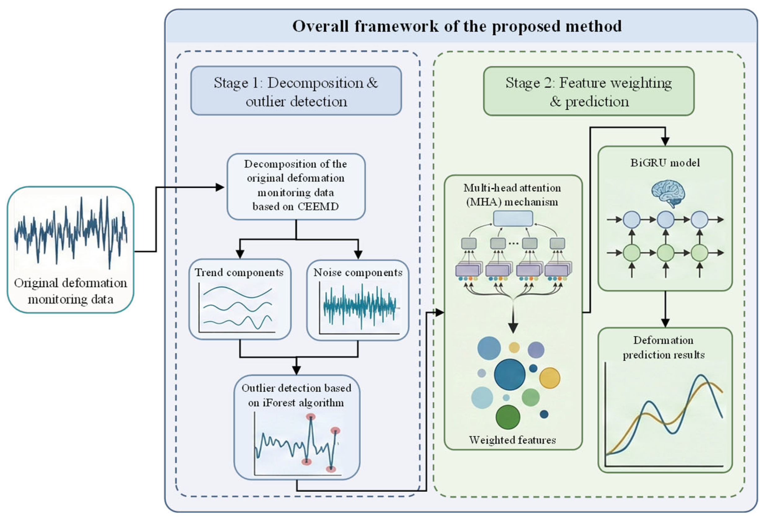
The rest of the presented study is arranged as follows. In Section 2, the outlier detection method of dam deformation monitoring sequences is explored by utilizing CEEMD and the iForest algorithm. Section 3 introduces the architecture of the MHA-BiGRU model. Section 4 introduces the initial monitoring data from a real-world hydraulic project to validate the efficacy of the proposed MHA-BiGRU prediction model. Then, six additional models are introduced. The analysis results of the forecasting results of all models are compared and discussed. Section 5 concludes the study and provides key directions for further research. This study presents an integrated framework spanning from data cleaning to deformation prediction, providing a new paradigm for the field of dam deformation prediction. The complete procedure of the proposed method is demonstrated in Figure 1.

2. Outlier Detection Method Based on CEEMD-iForest

2.1. Decomposition of the Original Deformation Sequence Based on CEEMD

The CEEMD method can be regarded as an extension of the EMD approach. EMD is well suited for non-stationary signal analysis because it adaptively decomposes a signal into multiple intrinsic mode functions (IMFs) at different characteristic scales, together with a residual term. Each IMF is required to meet two criteria: (1) the quantity of local extrema (maxima and minima) must correspond to the number of zero crossings or diverge by no more than one; and (2) at each given moment, the average value of the upper and lower envelopes, created by interpolating the local maxima and minima, must equal zero. Therefore, the original deformation sequence decomposition process is as follows:
m 1 t = X min t + X max t / 2
h 1 t = X t m 1 t
r 1 t = X t I M F 1
X t = i = 1 n I M F i + r n t
where X t represent the original deformation monitoring sequence, X min t and X max t denote the lower and upper envelopes, respectively, and r t represents the residual data sequence.
If h 1 t meets the requirements of the intrinsic mode function (IMF), it is taken as the first IMF and denoted as IMF1. The residual data sequence r t is then further decomposed by repeatedly applying Equations (1)–(3), and the process continues iteratively until the final residual r n t falls below a predefined threshold, at which point the decomposition terminates. If h 1 t does not meet the IMF criteria, it is further processed using Equations (5) and (6), and evaluated based on the condition described in Equation (7).
h 11 t = h 1 t m 11 t
h 1 k t = h 1 ( k 1 ) t m 1 ( k 1 ) t
t = 0 T h 1 ( k 1 ) ( t ) h 1 k ( t ) 2 h 1 ( k 1 ) 2 ( t ) < ε
where the parameter ε typically ranges from 0.2 to 0.3. However, when employing the Empirical Mode Decomposition (EMD) method for data sequence decomposition, the issue of mode mixing often arises, leading to decomposed components that may not accurately capture the intrinsic characteristics of the original data sequence. To overcome this limitation, Equations (8) and (9) are supplemented by paired positive and negative white-noise realizations by CEEMD, which effectively alleviates mode mixing.
x i + ( t ) = X ( t ) + n 1 ( t )
x i ( t ) = X ( t ) n 1 ( t )
I M F j = 1 2 N k = 1 n I M F j k + + I M F j k
where n1(t) means white noise.
After CEEMD, a continuous and smooth trend term, as well as an irregular and rapidly varying noise term, can be obtained by aggregating the corresponding intrinsic mode function (IMF) components. The threshold between the trend and noise terms can be determined using the Mean Standardized Absolute Mean (MSAM). Specifically, if the MSAM value at scale i exhibits a significant deviation from those at other scales, it can be inferred that, from this scale onward, the sum of the residual signal and the low-frequency IMF components constitutes the trend term. The MSAM for each IMF component can be expressed as:
MSAM [ i ] = m e a n i m f s [ i ] × i m f s [ i ] m e a n i m f s i s t d i m f s i
where std(imfs[i]) denotes the sample standard deviation.

2.2. iForest Algorithm

The Isolation Forest (iForest) algorithm partitions the feature space of the sample set through randomly generated trees, thereby isolating gross error points one by one. This approach detects anomalies based on two key characteristics of outliers: their sparse distribution and their considerable distance from dense clusters. Using a random sampling strategy, a specified number of isolation trees (iTrees) are constructed, which together form the isolation forest (iForest). The basic procedure of the iForest algorithm [40] is as follows:
(1) Training a single tree.
From the training dataset, a subset of ψ points is randomly selected and assigned to the root node of the isolation tree. A feature (dimension) is randomly chosen, and a cut point p is randomly generated within the range between the maximum and minimum values of the selected feature for the current node data di. Based on the cut point p, the dataset di is split into left and right subsets (left child: di < p; right child: di > p). The subset with fewer instances is then chosen as the new leaf node for the next iteration. This process continues until a leaf node contains only a single data instance or multiple identical instances (making further partitioning impossible), or until the tree reaches the predefined maximum depth.
(2) Aggregating the results from all isolation trees.
Each isolation tree (iTree) is traversed to compute the path length h(x) of the target sample in that tree. The mean of these values represents the expected path length E(h(x)) of the sample within the entire forest. For a subsample containing ψ instances, the structure of an iTree is equivalent to that of a binary search tree (BST). Consequently, the average path length of an unsuccessful search in the subsample is equivalent to the average unsuccessful search path length in a BST [41]:
c ψ = 2 H ψ 1 2 ψ 1 ψ
where H(ψ − 1) denotes the harmonic number, which can be approximated as ln(ψ − 1) + γ, and γ means the Euler–Mascheroni constant.
For each sample x, the results from all isolation trees are combined to compute its anomaly score as follows:
s x , ψ = 2 E h x c ψ
(3) Outlier detection
The detected data are classified according to the following criteria: When E(h(x))→c(ψ), the anomaly score s→0.5, indicating that the sample exhibits no significant abnormality. When E(h(x))→0, the anomaly score s→1, indicating that the sample is an outlier. When E(h(x))→ψ − 1, the anomaly score s→0, indicating that the sample is valid monitoring data.

2.3. The Process of the Proposed Outlier Detection Method

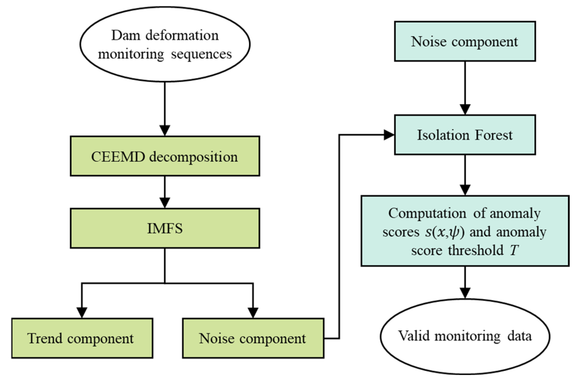
The CEEMD–iForest algorithm is a time series outlier detection approach that integrates signal decomposition with machine learning techniques. First, the CEEMD method is utilized in the dam deformation monitoring time series to decompose the signal and extract both the trend and noise components. Subsequently, the Isolation Forest (iForest) algorithm is employed to process the noise component and identify anomalies within the sequence. This method utilizes the intrinsic scale-adaptive characteristic of CEEMD, exhibiting resilience and clarity in the analysis of nonlinear and non-stationary time series data. The detailed workflow of the CEEMD–iForest outlier detection algorithm is illustrated in Figure 2.

3. Prediction Method Based on MHA-BiGRU Model

3.1. BiGRU Model

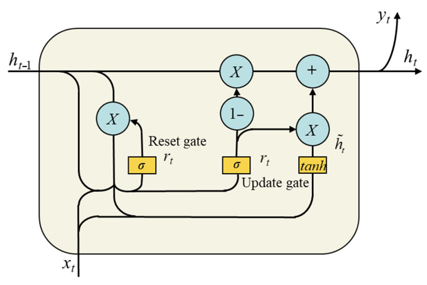
The GRU was developed to better preserve long-range dependencies and to alleviate vanishing gradients during backpropagation, which are common issues in standard RNNs [42]. The GRU utilizes an update gate and a reset gate internally. The update gate regulates the amount of useful information from the previous time step that is carried forward to the current step, while the reset gate determines the extent to which prior information should be discarded. Owing to its reduced parameterization and simplified architecture, the GRU is capable of effectively learning from historical data. The structure of the GRU is illustrated in Figure 3.
These two gating mechanisms determine how much information is retained and how much is discarded, respectively. Their formulations are given as follows:
z t = σ W z h t 1 , x t
r t = σ W r h t 1 , x t
h ˜ t = tanh W h ˜ r t h t 1 , x t
h t = 1 z t h t 1 + z t h ˜ t
where z t , r t , h t represent the update gate, reset gate, and the current hidden state, respectively. Wz and Wr are the weight matrices corresponding to the update and reset gates, while W h ˜ denotes the weight matrix for computing the candidate hidden state.
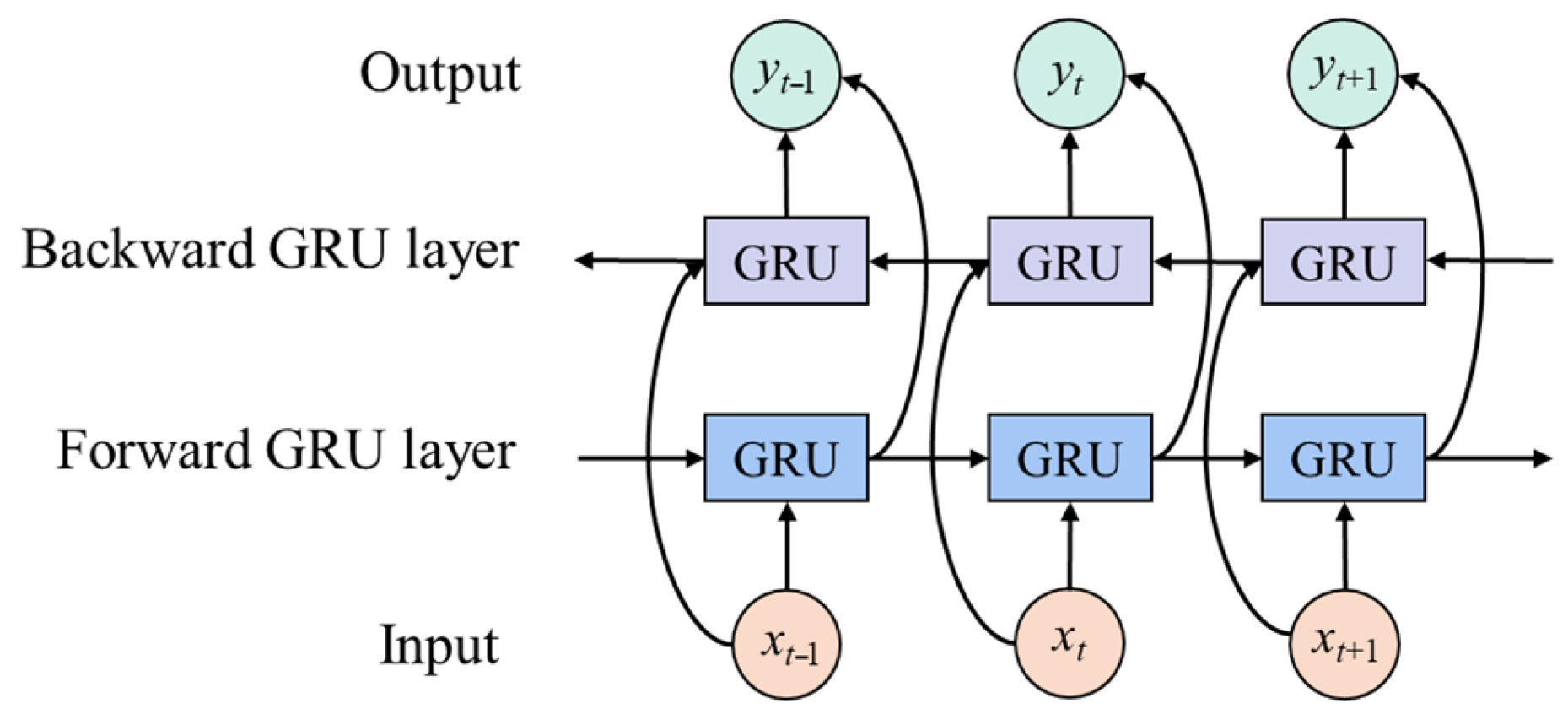
The BiGRU extends the standard GRU by processing sequences in both forward and backward directions [43]. It consists of a forward GRU layer and a backward GRU layer, which are designed to learn within-window contextual information during the forward pass and past information during the backward pass, respectively. Compared to the unidirectional GRU that processes information in only one direction, the bidirectional architecture of BiGRU more effectively captures long-term dependencies within time series data, thereby improving the predictive performance of the model and reducing prediction errors. The architecture of BiGRU is illustrated in Figure 4.
The mathematical representation of the BiGRU network is expressed as follows:
h t = GRU x t , h t 1
h t = f W h t h t + W h t h t + b t
where h t and h t stand for the forward and backward hidden states at time step t, respectively, W h t and W h t denote the weights of the forward and backward hidden states at time t, respectively, and bt is the bias term of the hidden state at time t.

3.2. Multi-Head Attention Mechanism (MHA)

Humans usually focus more on information that appears most important, especially in complex settings. This observation has motivated the development of attention mechanisms, which allow neural networks to selectively emphasize the most relevant parts of the input during training. By assigning larger weights to key features, attention helps the model capture informative patterns in data with complex distributions. Among various attention-based methods, the self-attention mechanism has proven particularly effective in modeling internal dependencies within sequences. In the context of dam deformation forecasting, self-attention can identify the most relevant historical time steps within the input monitoring sequence that are most relevant to the prediction task, dynamically adjusting their weights to improve forecasting accuracy.
The MHA mechanism can be regarded as an extension of self-attention. Instead of relying on a single attention representation, MHA employs multiple parallel self-attention heads, each attending to different subspaces or aspects of the input. This design enables the model to extract richer and more varied features from different perspectives, thereby improving representation quality and generalization performance. The underlying principle of MHA is described as follows:
Attention ( Q , K , V ) = softmax Q K T d k V
head i = Attention ( Q i , K i , V i )
MultiHead ( Q , K , V ) = Concat ( head 1 , , head h ) W O
where Q, K and V mean the query, key, and value matrices, respectively. The output of the i-th attention head is represented as headi, and the final output of the multi-head attention mechanism is denoted as MultiHead(Q,K,V).

3.3. The Overall Architecture of the Presented Prediction Model

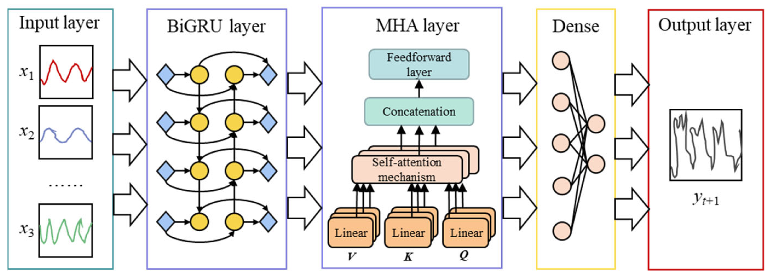
Figure 5 illustrates the architecture of the proposed MHA-BiGRU prediction model, which comprises three critical components: the input layer, the representation layer, and the output layer sequentially.
The impact factors affecting dam deformation make up the input layer, while the output layer corresponds to the predicted dam deformation values. The representation layer embodies the model’s computational process and is primarily composed of the BiGRU subnetwork and the MHA subnetwork connected in series. The BiGRU subnetwork comprises one layer of bidirectional GRU networks, which take both the forward and backward gated recurrent neural networks as inputs. The layer is designed to capture historical data patterns and within-window contextual information, respectively. The BiGRU subnetwork successfully captures bidirectional information flow inside time-series datasets by combining the outputs of the layer using both past and next-node data. However, as the length of the input sequence increases, the fixed-length context vector becomes insufficient to represent the true information in the data, leading to potential information loss and difficulty in extracting high-dimensional features.
The MHA subnetwork applies multiple distinct linear mappings to the outputs of the BiGRU subnetwork and computes the corresponding attention matrices. The outputs from multiple attention heads are concatenated and linearly projected to form the final multi-head attention representation. This operation captures temporal dependencies across multiple subspaces and yields attention weights for different features. The MHA subnetwork emphasizes the importance of key features in the model’s prediction, highlighting strongly correlated features while diminishing the influence of weakly correlated ones. This enables the capture of critical factors affecting dam deformation prediction. The combination of the two subnetworks enhances the learning capability and addresses the accuracy degradation caused by long time spans in dam deformation prediction tasks. The formula of the proposed prediction method is illustrated as:
y t + 1 = M H A X W Q , X W K , X W V
X = B i G R U x T
where yt+1 means the prediction value of dam deformation at time t + 1, xT represents the input monitoring data of impact factors x1, x2, …, xt, X is the output vector of the BiGRU subnetwork, and WQ, WK, and WV are the parameter matrices.

4. Case Study

4.1. Overview of the Studied Project

One medium-scale hydropower station is located on the stream of the Hongshui River in the Guangxi Zhuang Autonomous Region, China. The most important function of the project is power generation, with additional roles in flood control and navigation. The total installed capacity of the station is 4900 MW.
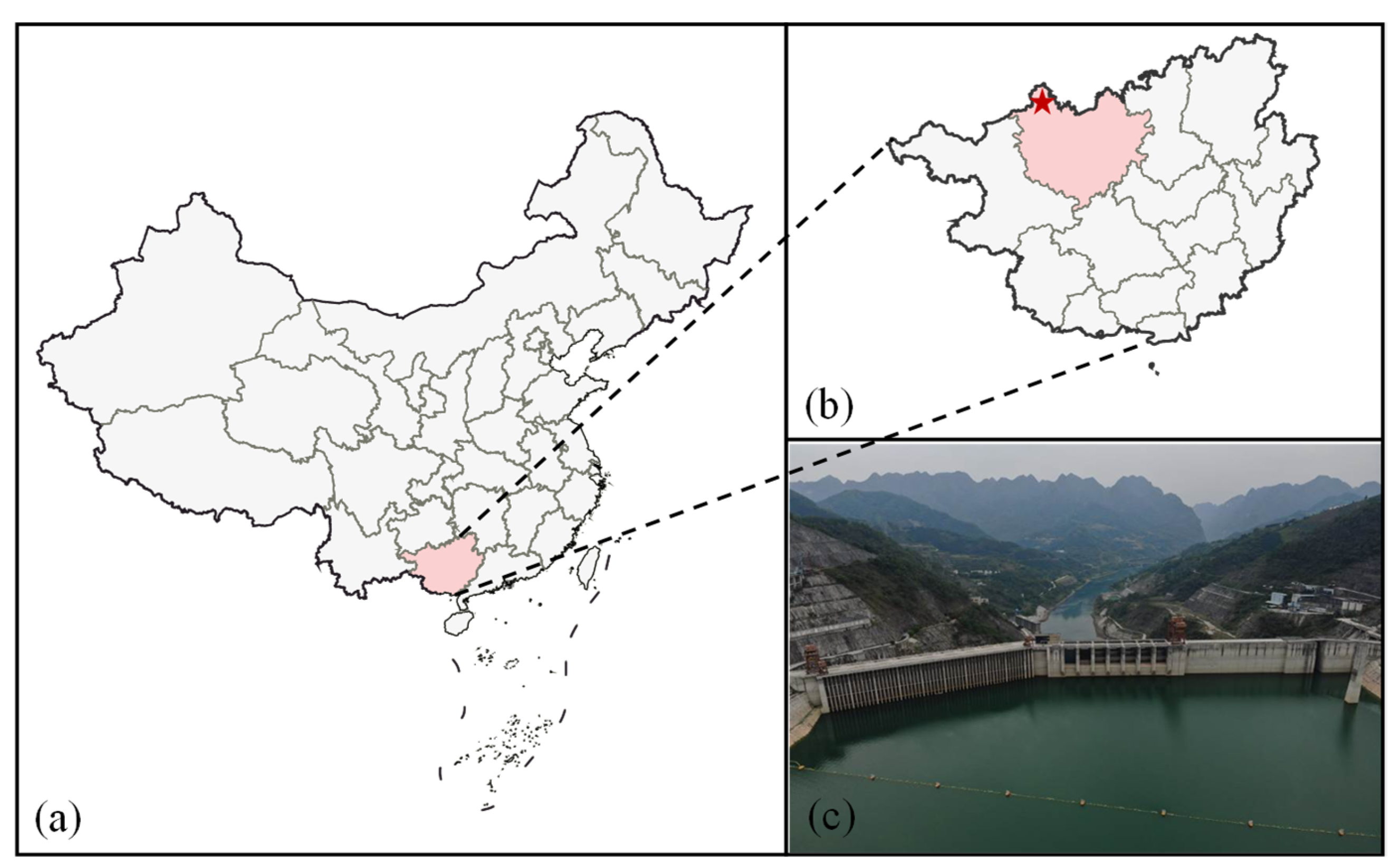
In the first phase of construction, the reservoir operates with a normal storage level of 375 m, a dead water level of 330 m, a flood control limit level of 359.3 m, a design flood level of 377.26 m, and a check flood level of 381.84 m. The total storage capacity of the reservoir is 18.809 billion m3, with an effective storage capacity of 11.15 billion m3. It serves as an annual regulation reservoir, with a guaranteed output of 1234 MW and an average annual power generation of 15.67 billion kWh. As depicted in Figure 6, the photograph of the geographical location of the dam project and representative site is presented. The red star in Figure 6 indicates the approximate location of the project on the map.
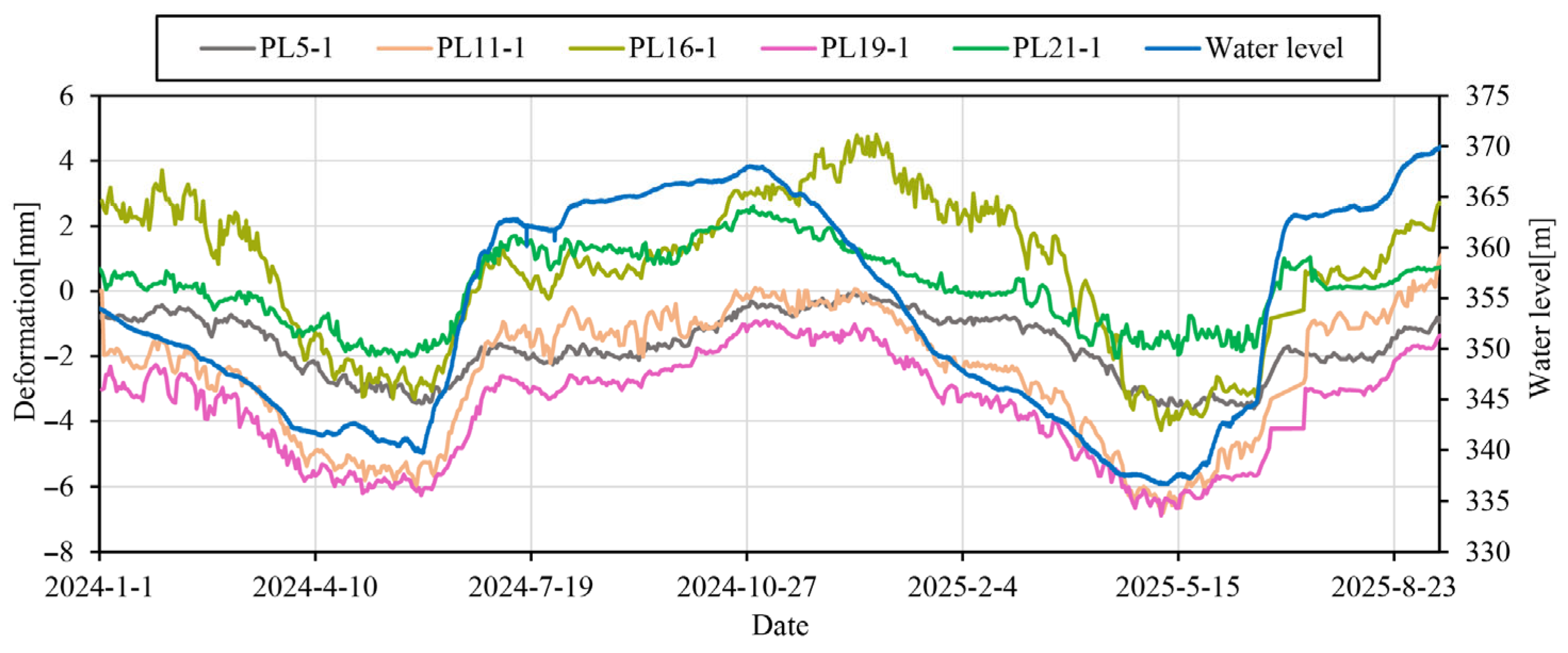
Combined plumb line systems were installed at six representative dam sections (Nos. 5, 11, 16, 19, 21, and 32). The monitoring system consists of 8 inverted plumb lines and 15 direct plumb lines, with a total of 28 deformation monitoring points. Radial deformation monitoring data of five representative monitoring points located along the vertical alignment of different dam sections are selected for analysis. Figure 7 demonstrates the process lines of radial deformation monitoring sequences without outliers of points PL5-1, PL11-1, PL16-1, PL19-1, and PL21-1 from 1 January 2024 to 19 September 2025, and the relevant monitoring data of the upstream water level.

4.2. Outlier Detection Results Analysis

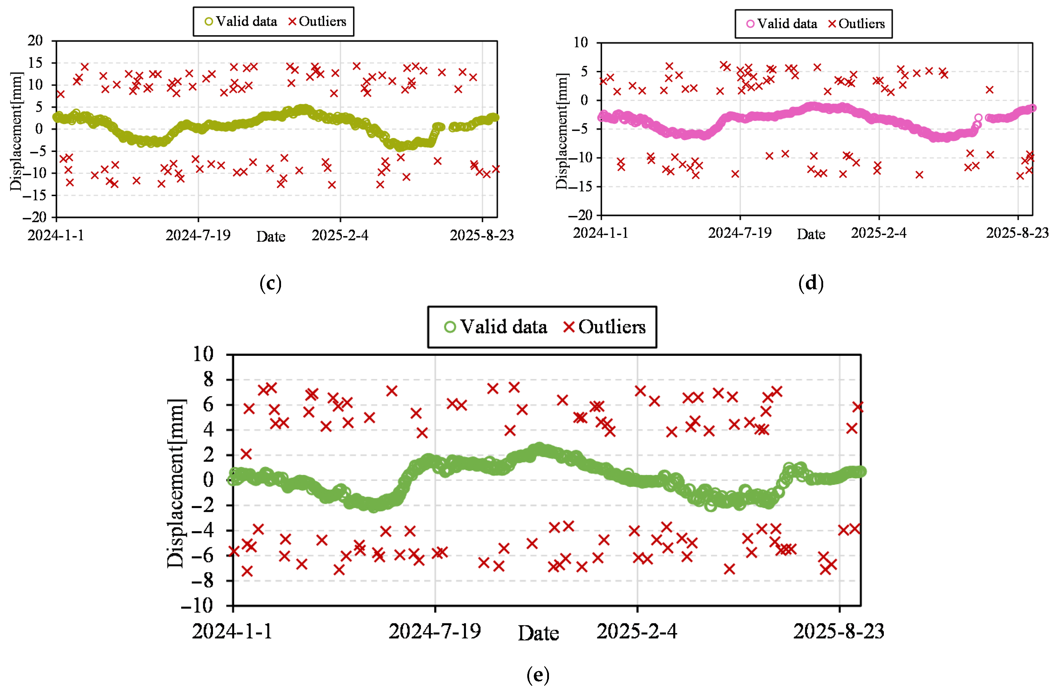
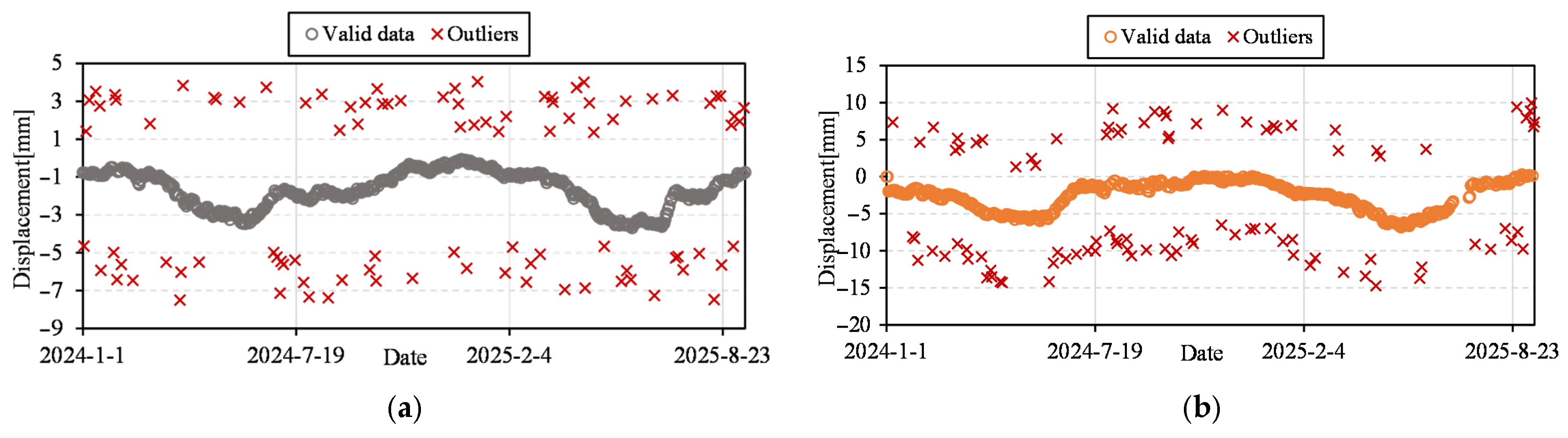
We generated a random error sequence following a normal distribution N ( 0 , σ 2 ) , where σ is the standard deviation of the valid monitoring series. To simulate various levels of anomalies, we specifically extracted and injected errors with magnitudes ranging from 2 σ to 3 σ into the original data. This magnitude range is highly representative of real-world sensor anomalies. 2 σ errors simulate subtle environmental fluctuations or sensor drifts that push the data to the edge of the 95.4% confidence interval. 3 σ errors represent significant outliers or impulse interference, which are typical in cases of sensor malfunction or extreme transient events. The outliers were randomly distributed across the time series with a total contamination rate of about 20%. This rate simulates real-world monitoring environments, especially during periods of sensor degradation or severe environmental interference. Figure 8 depicts the monitoring sequences for each monitoring point, including outliers. Table 1 displays the number of valid data and outliers of all the selected monitoring points.
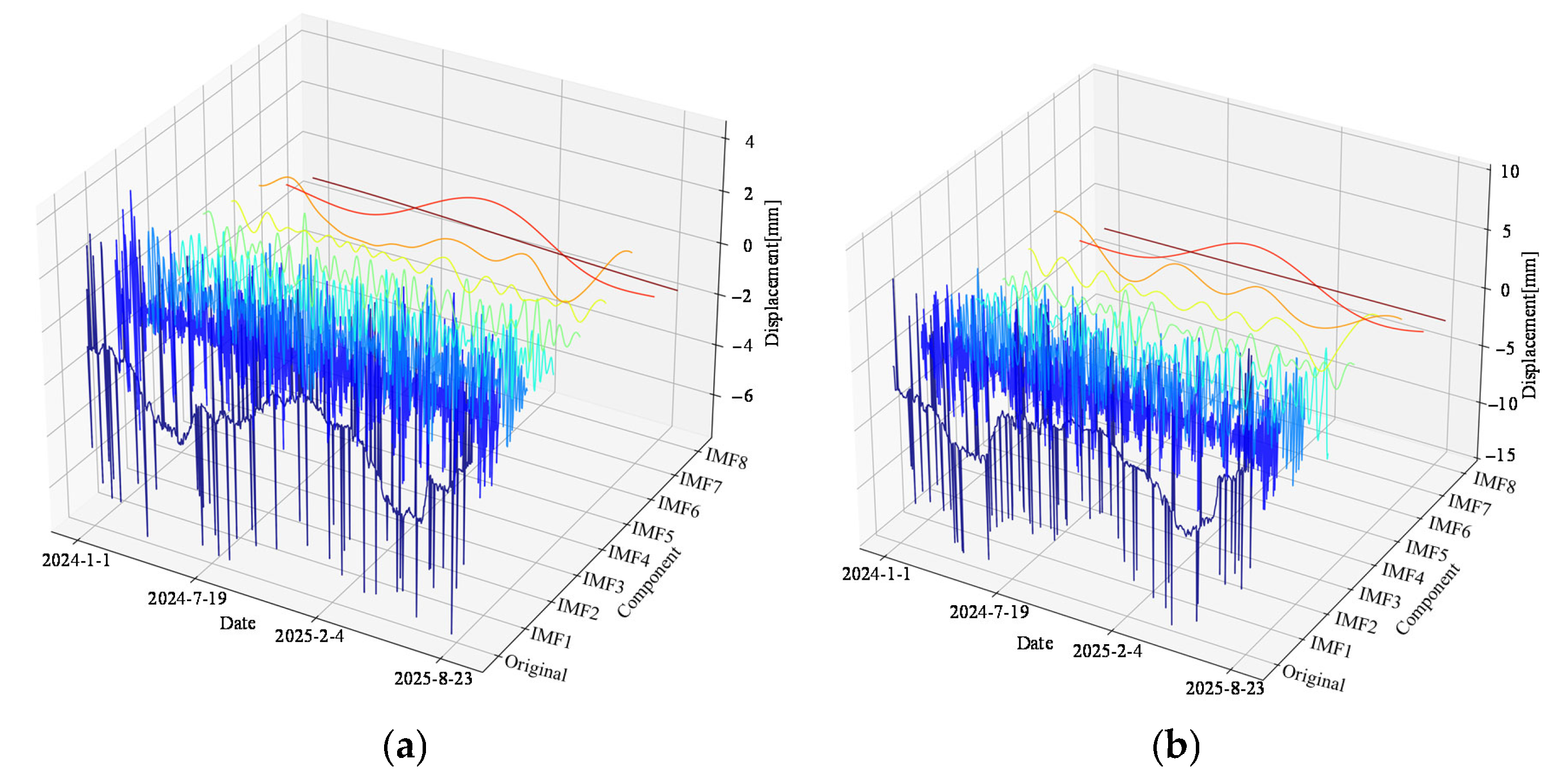
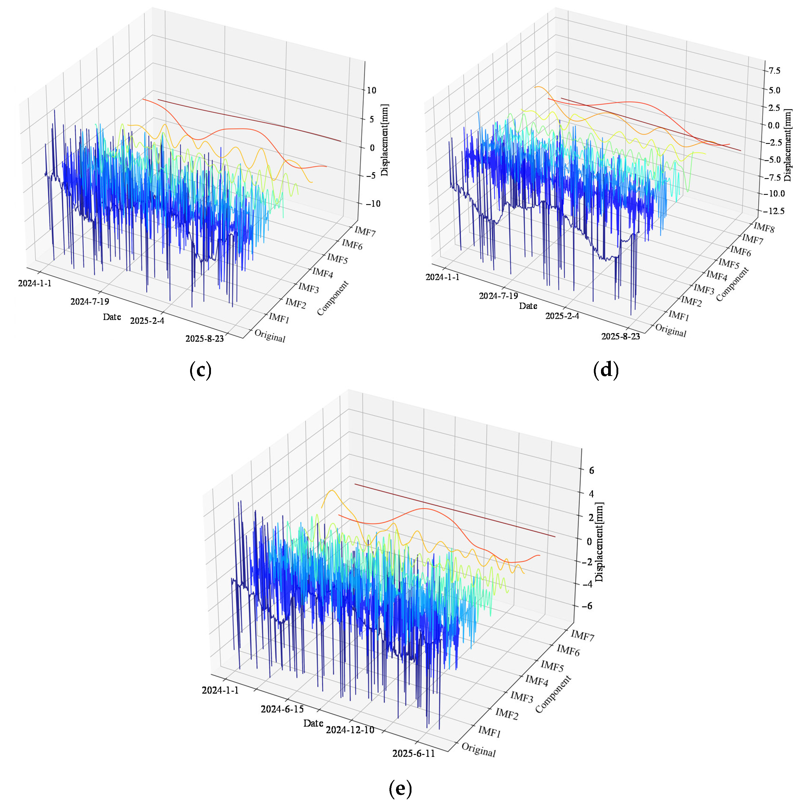
Figure 9 illustrates the decomposition of the original signals of five monitoring points into intrinsic mode functions (IMFs) at various levels using CEEMD.
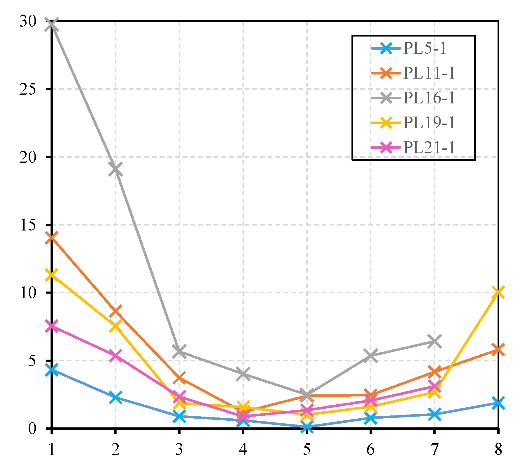
Figure 10 summarizes the mean squared amplitude modulation (MSAM) of each IMF component. As shown in Figure 10, on the basis of the minimum MSAM criterion, the MSAM values for monitoring points PL5-1, PL16-1, and PL19-1 reached their minimum at IMF5. This indicates the end of high-frequency noise. Therefore, the trend components for these points were reconstructed starting from IMF6. For monitoring points PL11-1 and PL21-1, the MSAM value reached its minimum at IMF4. Consequently, its trend component was reconstructed starting from IMF5. This variation in cutoff points across different monitoring points confirms that the proposed selection rule is data-driven and adaptive, allowing the model to automatically determine the optimal noise–trend boundary based on the intrinsic frequency characteristics of each specific monitoring sequence.
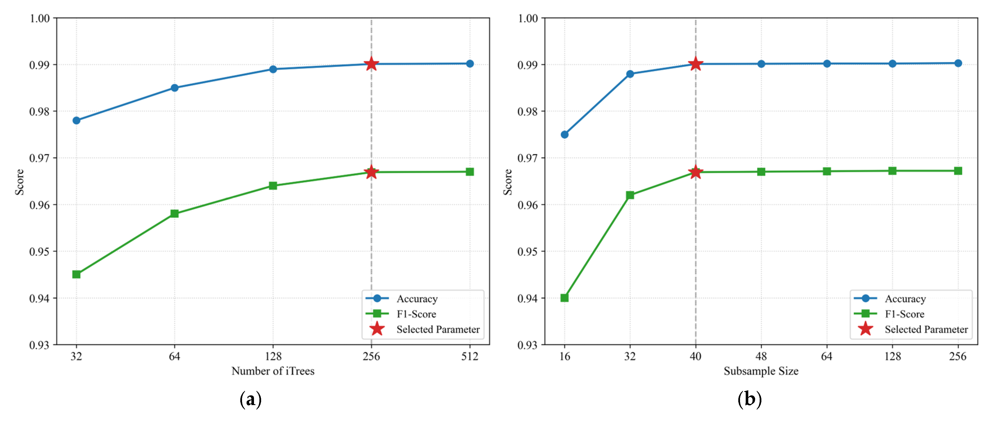
Additional tests to evaluate the impact of various iForest parameters on outlier detection performance using the control variable method were conducted. Figure 11a illustrates the average values of accuracy and F1-Score of outlier detection results across five monitoring points under different numbers of itrees. Figure 11b shows the average values of the accuracy and F1-Score across the same five monitoring points under different subsample sizes. In each test, we varied one specific parameter across a wide range while keeping the other parameters fixed at their optimal values (indicated by the red stars in Figure 11).
When keeping the subsample size fixed at 40, we varied the number of trees from 32 to 512. The results show that performance stabilizes after 256 trees. While keeping the number of trees fixed at 256, we varied the subsample size from 16 to 256. A size of 40 was found to be sufficient for consistent performance. Since the tree height in the iForest algorithm is natively determined by the subsample size, the analysis of the subsample size inherently covers the sensitivity of tree height. Similar trends were observed across multiple datasets with varying outlier densities.
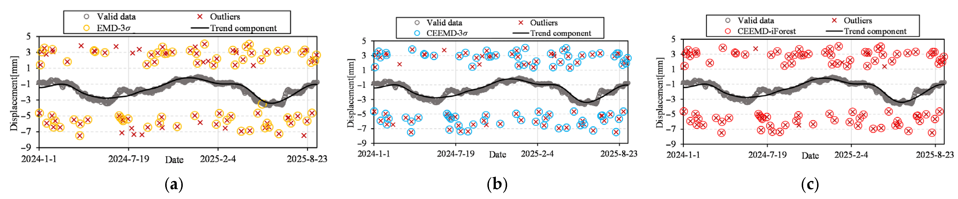
In this study, outlier detection for the five monitoring points was performed using the CEEMD-iForest method, the CEEMD-3σ method, and the EMD-3σ method, and the results of the three approaches were comparatively analyzed. Different parameter settings reflect the performance and efficiency of the model. In the isolation forest algorithm, the data features were adjusted and optimized, with the maximum decomposition level set to five, the sample size for each iTree set to 40, and the maximum tree height limited to five. The entire forest comprised 256 iTrees, and the anomaly score discrimination threshold was set to 0.5 mm. The outlier detection results of the above three methods for PL5-1 are presented in Figure 12.
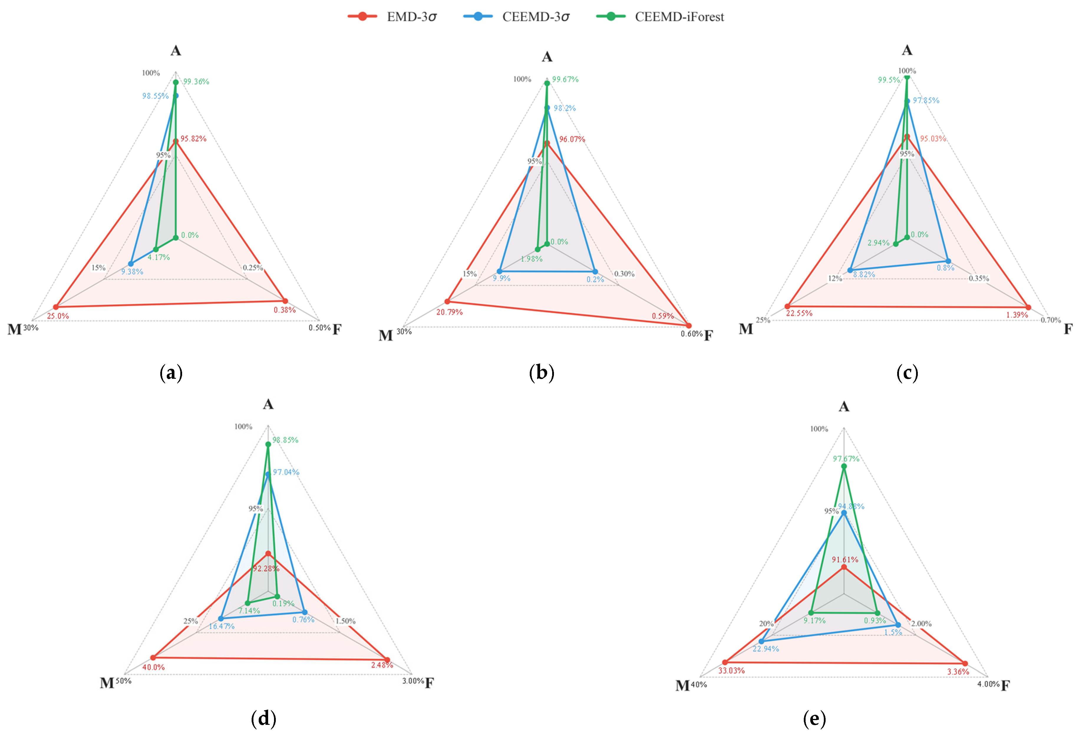
To evaluate the efficiency of outlier detection, three evaluation metrics, Accuracy (A), missed detection rate (M), and false detection rate (F), are utilized in this case study. The evaluation metrics can be calculated as follows:
A = n T T + n F F n T T + n F F + n F T + n T F
M = n F T n F F + n F T
F = n T F n T T + n T F
Considering the class imbalance between normal data and outliers in dam monitoring sequences, accuracy alone may not fully reflect the detection performance. Therefore, Precision, Recall, and F1-Score are introduced to provide a more comprehensive evaluation. Precision measures the proportion of actual outliers among all points identified as anomalies, while Recall measures the proportion of actual outliers that are correctly detected. The F1-Score is the harmonic mean of Precision and Recall, serving as a balanced metric. These evaluation metrics are calculated as follows:
P r e c i s i o n = n F F n F F + n T F
R e c a l l = n F F n F F + n F T
F 1 S c o r e = 2 × P r e c i s i o n × R e c a l l P r e c i s i o n + R e c a l l = 2 × n F F 2 × n F F + n T F + n F T
where nTT denotes the number of data correctly identified as valid data, nFF means the number of abnormal points correctly identified as outliers, nFT is the number of abnormal points incorrectly identified as valid data, and nTF represents the number of normal points incorrectly identified as outliers. Accuracy represents the proportion of correctly identified points. The missed detection rate M is defined as the proportion of abnormal points misclassified as normal to the total number of outliers, reflecting the method’s ability to detect actual outliers. The false detection rate F is defined as the proportion of normal points misclassified as abnormal to the total number of valid data, reflecting the method’s ability to correctly recognize actual valid data.
The statistical results of outlier detection for monitoring data from five monitoring points are demonstrated in Table 2. And the outlier detection performance evaluation metrics are depicted in Figure 13 and Table 3.
As exhibited in Figure 12, for point PL5-1, the CEEMD-iForest method outperformed the CEEMD-3σ method in terms of accuracy (99.36%), missed detection rate (4.17%), and false detection rate (0.00%), achieving an improvement in outlier detection rate. Meanwhile, the CEEMD-3σ method demonstrated higher accuracy and lower missed detection rate (98.55% and 9.38%, respectively) than the EMD-3σ method (95.82% and 25.00%), with a marginal increase in false detection rate (0.00% vs. 0.38%).
In comparison to the EMD-3σ and CEEMD-3σ methods, for all the tests, the proposed CEEMD-iForest method outperforms them in each evaluation metric. Specifically, regarding the accuracy (A), the CEEMD-iForest algorithm consistently achieves the highest values, reaching 99.67% in the test cases, which indicates its robustness in distinguishing between outliers and normal fluctuations. A substantial improvement is observed in the miss rate (M). For all the monitoring points, the conventional EMD-3σ method suffers from a high miss rate, and the CEEMD-3σ method reduces this rate. Remarkably, the CEEMD-iForest method further suppresses the miss rate, demonstrating its exceptional sensitivity to subtle outliers. Furthermore, the False Alarm Rate (F) of the proposed method is effectively minimized, ensuring that valid data points are preserved to the maximum extent.
To quantitatively evaluate the efficacy of the proposed outlier detection framework, Table 3 presents a comparative analysis of three methods: EMD-3σ, CEEMD-3σ, and the proposed CEEMD-iForest. The evaluation utilizes Precision, Recall, and F1-Score across five distinct monitoring points to assess performance under varying signal characteristics.
As evidenced in Table 3, the proposed CEEMD-iForest method consistently outperforms the baseline approaches by a substantial margin across all metrics. The proposed method achieves the highest F1-Scores at all monitoring points, ranging from 92.96% to 99.00%. Notably, at point PL19-1, where signal complexity is presumably higher, the EMD-3σ method struggles with an F1-Score of only 68.46%. In contrast, CEEMD-iForest maintains a robust performance of 95.12%, demonstrating a significant improvement of approximately 26.6%. This indicates the proposed method’s exceptional capability in handling class imbalance and complex noise patterns. The proposed method exhibits near-perfect precision, reaching 100% at PL5-1, PL11-1, and PL16-1. This suggests that the inclusion of the iForest algorithm effectively eliminates false alarms caused by fluctuating noise, ensuring that identified anomalies are genuine structural responses rather than noise artifacts.
Compared to the 3σ threshold, the iForest-based approach significantly boosts Recall rates. For instance, at PL21-1, the Recall improves from 66.97% to 90.83%. This confirms that the proposed method effectively mitigates the “masking effect,” successfully identifying subtle outliers that traditional statistical methods might miss. Overall, the values of all the evaluation metrics confirm the comprehensive superiority and engineering applicability of the CEEMD-iForest framework.

4.3. Prediction Results Analysis of MHA-BiGRU Model

Based on the outlier detection results for the radial deformation monitoring data from five monitoring points, the dataset was divided into training and test sets at an 8:2 ratio. Specifically, the first 80% of the monitoring sequence was used for training, while the remaining 20% was reserved for testing. Based on the dam deformation statistical model, the input factors for the model were determined as: H, H2, H3, sin 2 π t 365 sin 2 π t 0 365 , cos 2 π t 365 cos 2 π t 0 365 , sin 4 π t 365 sin 4 π t 0 365 , cos 4 π t 365 cos 4 π t 0 365 , θ θ 0 , and ln θ ln θ 0 . Among them, H means upstream water level, t represents time corresponding to the current monitoring value, t0 is time corresponding to the initial monitoring value, and θ = t / 100 . The physical interpretation of the above input factors is as follows:
(1) Hydrostatic component (H, H2, H3): These terms represent the elastic deformation caused by water pressure. The polynomial expansion accounts for the non-linear relationship between the upstream water level and the dam deformation characteristics.
(2) Thermal component (harmonic terms): The sine and cosine functions simulate the dam deformation driven by seasonal ambient temperature changes.
(3) Aging component ( θ , ln θ ): These time-dependent terms capture the irreversible deformation caused by concrete creep and foundation consolidation.
To verify the superiority of the proposed method, this study compares it with six baseline models: the traditional LSTM model, the standard GRU model, the BiGRU model, the CEEMD-LSTM model, the eXtreme Gradient Boosting (XGBoost) model, and the TCN (Temporal Convolutional Network) model. To ensure a fair comparison, key training-related hyperparameters, including the look-back window, learning rate, batch size, optimizer, and loss function were kept identical across all models. Model-specific structural hyperparameters were tuned via independent grid search based on the training data.
For the baseline LSTM, GRU, BiGRU, and CEEMD-LSTM models, the best-performing configurations selected by grid search employed a hidden size of 64 and a dropout rate of 0.2, providing sufficient representation capacity. The TCN model was configured with 64 filters to maintain comparable representation capacity, while XGBoost parameters were tuned separately. Conversely, superior overall performance was attained by the MHA–BiGRU framework, configured with a reduced hidden dimension and an elevated dropout rate. This finding suggests that efficient feature extraction is facilitated by the integration of multi-head attention, necessitating fewer recurrent units. Furthermore, the increased model complexity arising from attention parameters is effectively mitigated through robust dropout regularization. To ensure the reproducibility of the experiments, all hyperparameters and implementation details are summarized in Table 4. Mean squared error (MSE) was adopted as the loss function for model training.
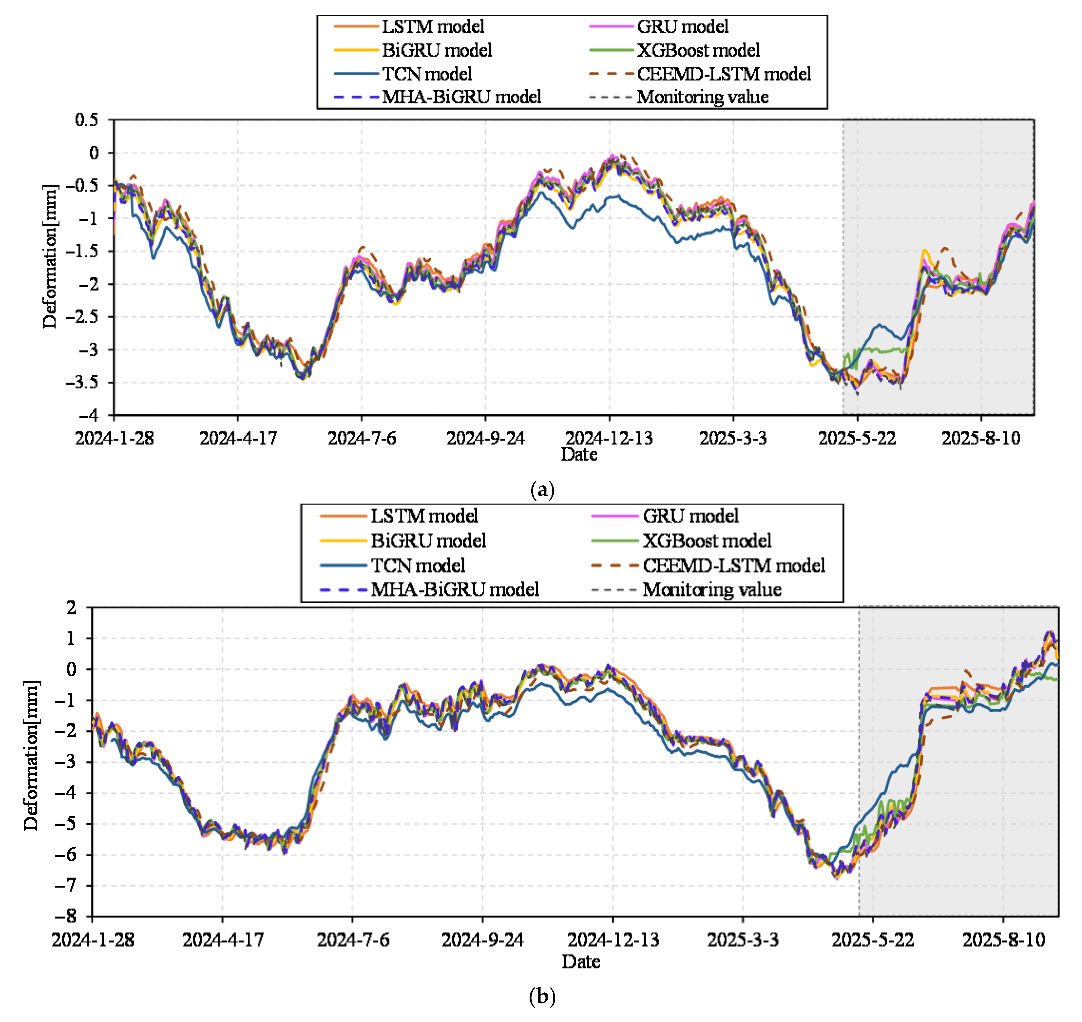
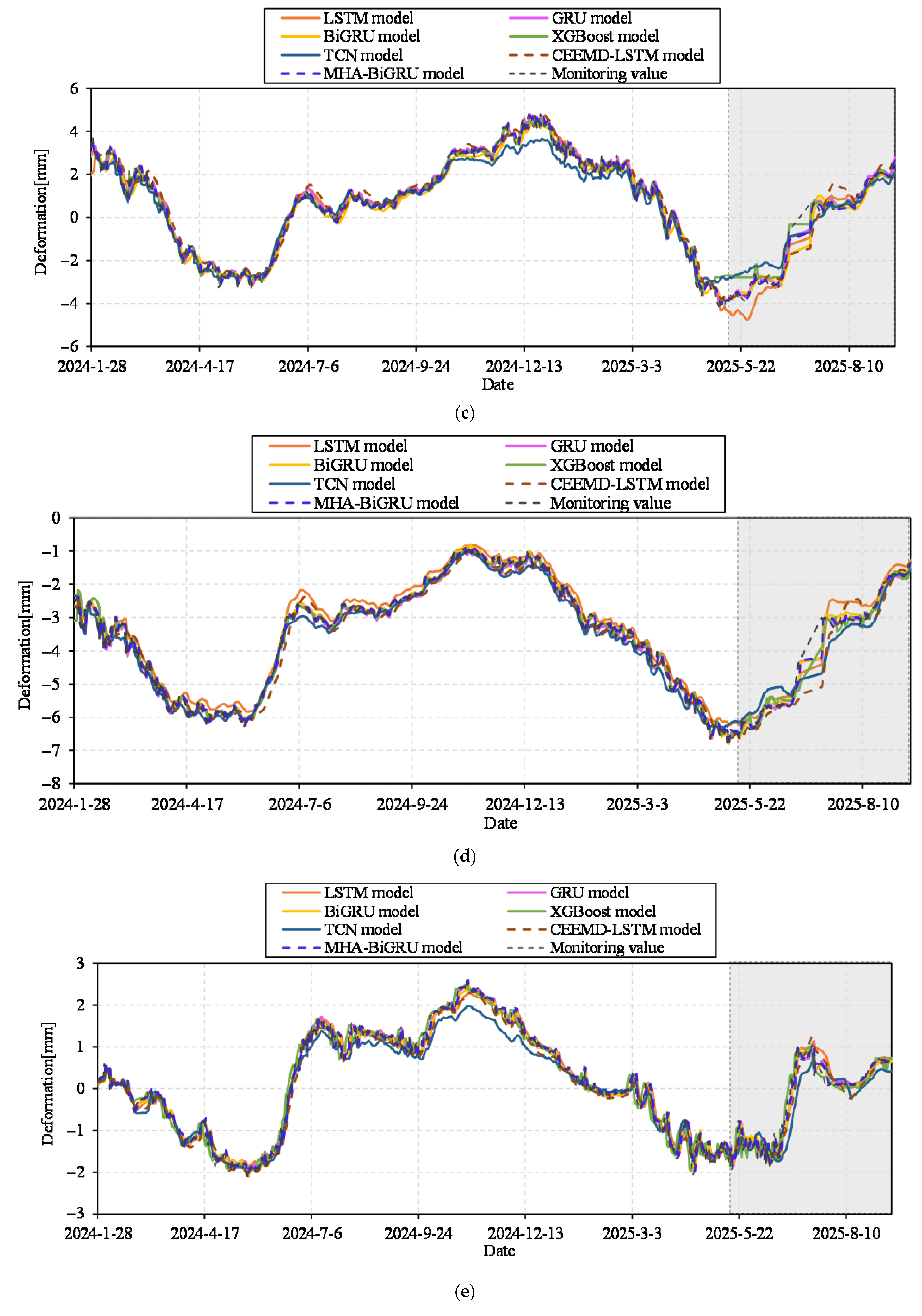
Based on the monitoring data from the selected five monitoring points, the model was established and used for prediction. The fitting and prediction results of the selected five monitoring points are depicted in Figure 14. The gray box in Figure 14 highlights the model prediction results.
Figure 14 shows that the proposed model’s fitting and forecasting results match the actual monitoring sequences quite well, proving once again how much better it is. Furthermore, to quantitatively evaluate the model performance, both the root mean squared error (RMSE), the coefficient of determination (R2) and mean absolute error (MAE) were employed to comprehensively assess the model’s fitting accuracy and generalization performance [44]. The specific calculation formulas are written as:
R 2 = i = 1 N δ ^ i δ ¯ i = 1 N δ i δ ¯
R M S E = 1 M j = 1 M δ j δ ^ j 2
M A E = 1 M j = 1 M δ j δ ^ j
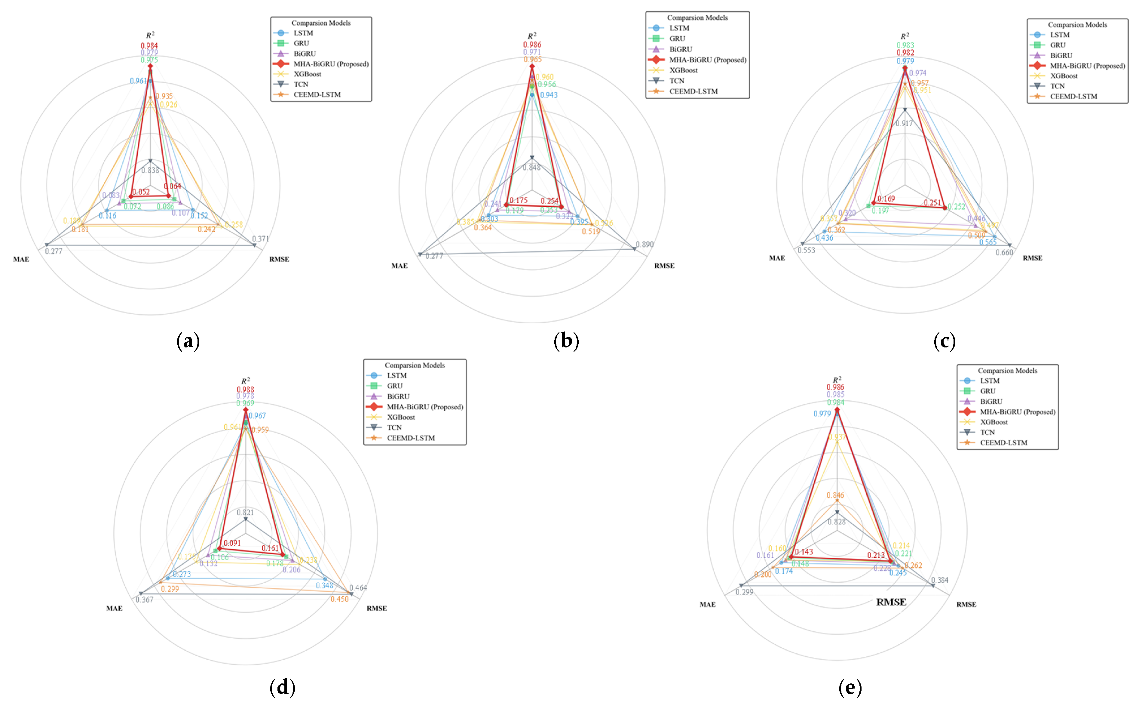
where δ i means the monitoring values of the training sets, δ ¯ means the average value of the sum, δ ^ i represents the fitted deformation values of the training sets, δ j is the monitoring deformation values, δ ^ j is the prediction deformation values of the testing sets, and N and M are the data number of training and forecasting datasets, respectively. Finally, in Figure 15, the R2, RMSE and MAE metrics of the four comparative models are shown.
The comparative analysis of the four models, based on data from five monitoring points, indicates that the MHA-BiGRU model exhibits optimal overall performance and robustness across all tests. As shown in Figure 14, this model demonstrates high goodness of fit and low error. Its R2 values remain consistently above 0.982. Furthermore, even when the LSTM, TCN and CEEMD-LSTM models exhibit significant error fluctuations, the MHA-BiGRU model maintains errors at a low level. The GRU, BiGRU and XGBoost models demonstrate intermediate performance, while BiGRU is slightly superior in capturing contextual dependencies, and the GRU model exhibits better generalization in specific scenarios due to its simpler structure.
To mitigate the uncertainty introduced by random initialization and other stochastic training procedures in neural networks and to evaluate model stability, we conducted 10 independent runs for each model using the same time-ordered training, validation, and test split and identical hyperparameters, while varying only the random seed. Taking PL5-2 as an example, Table 5 demonstrates the mean ± standard deviation of RMSE, MAE, and R2.
Table 5 summarizes the results over 10 independent runs. MHA-BiGRU achieves the best average performance and demonstrates the smallest run-to-run variation, indicating stable predictive behavior. In contrast, several baselines, such as TCN, LSTM, and CEEMD-LSTM exhibit noticeably larger variability across runs. XGBoost yields relatively consistent results under our setting. However, its overall prediction errors remain higher than those of MHA-BiGRU. The MHA mechanism explicitly reweights the BiGRU latent temporal representations within the look-back window, allowing the model to focus more on informative historical time steps and mitigating information dilution in longer sequences.

4.4. Visualization of Attention Weights and Interpretability Analysis

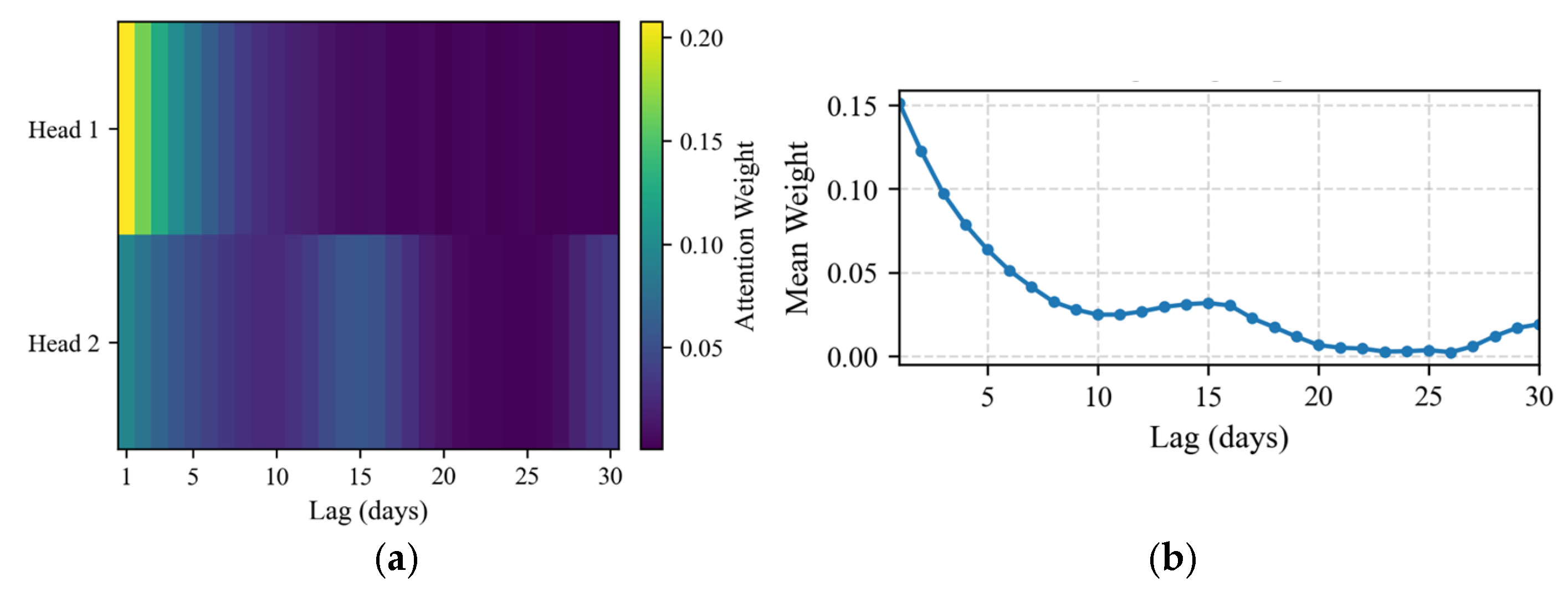
To enhance interpretability, we analyze the attention matrices produced by the MHA subnetwork. For each head h, the attention matrix is A(h). For one-step-ahead prediction, we focus on the query corresponding to the last time step of the input window and average the resulting weights across heads and test samples to obtain a lag-importance profile. Taking monitoring point PL5-1 as a case, we visualize it using a heatmap and a lag-importance curve in Figure 16. The averaged attention heatmap and the lag-importance curve are presented in Figure 16b, indicating that the model assigns higher weights to the most informative historical periods.
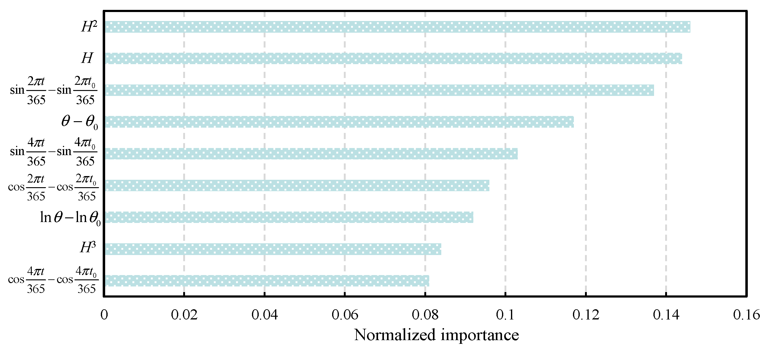
Since the MHA module is applied to the BiGRU latent temporal representations, attention weights mainly reflect the importance of key historical time steps, rather than directly corresponding to the contribution of raw input factors. For readability, the SHAP-based factor importance is normalized to demonstrate the contribution strength of each input factor to the model output. Taking monitoring point PL5-1 as a case, the normalized input factors’ importance based on SHAP is depicted in Figure 17.
Figure 17 summarizes the overall contribution strength of each input factor to the model output. For readability, the SHAP-based factor importance is normalized. Larger values indicate stronger overall influence on dam deformation prediction. Note that the plot reports factor-level importance aggregated over the input window. This analysis provides factor-level interpretability for the proposed model and is consistent with conventional statistical mechanisms involving water level terms, and temperature-related effects.

5. Discussion and Conclusions

In this study, we propose a novel dam deformation prediction method enhanced by an outlier detection framework. CEEMD is introduced to achieve multi-scale decomposition of deformation monitoring sequences, and iForest is subsequently employed to identify outliers mainly concentrated in the noise-dominant components. On the basis of outlier detection, the dam deformation prediction model based on MHA–BiGRU is trained using the reliable monitoring data. Overall, the proposed framework provides a systematic and practically applicable solution for real-world dam monitoring data analysis with strong engineering relevance. The main conclusions are as follows:
(1) The outlier detection method presented in this study was applied to four sets of dam monitoring data. The analysis results indicate that the CEEMD-iForest algorithm not only improves the outlier detection accuracy by increasing correct outlier identification rates, but also reduces false negatives and false positives, thereby providing technical support for dam deformation monitoring and early warning.
(2) For dam deformation prediction, the MHA–BiGRU model achieves superior accuracy and robustness compared with baseline models, validated through rigorous benchmarking. The bidirectional GRU captures temporal dependencies within the look-back window. And the multi-head attention module reweights the latent temporal representations to emphasize informative historical time steps, mitigating information dilution in long-span sequences. Furthermore, aligning with the stringent standards for safety-critical infrastructure, the proposed framework moves beyond “black-box” prediction. Factor-level interpretability is provided via SHAP-based importance analysis, which quantifies the relative contributions of input driving factors. This transparency ensures that the model’s behavior is physically explainable and trustworthy, significantly enhancing its credibility for practical engineering deployment.
(3) This study establishes an integrated workflow from multi-scale decomposition and outlier detection to deformation prediction. Although promising, the computational cost of CEEMD and model inference may increase with long sequences and high-frequency monitoring streams. Future work will focus on improving computational efficiency for real-time deployment, extending validation to more dams and monitoring conditions, and further enhancing interpretability beyond accuracy-oriented improvements.

Author Contributions

Conceptualization, J.X. and Y.S.; methodology, Y.S.; software, Y.S., J.L. and Z.J.; validation, B.C., C.M. and S.Z.; formal analysis, C.F.; investigation, J.X. and Y.S.; resources, J.X. and Y.S.; data curation, J.L.; writing—original draft preparation, J.X., Y.S., Z.J. and S.Z.; writing—review and editing, Y.S., C.F., B.C. and C.M.; visualization, B.C.; supervision, J.L.; project administration, J.X.; funding acquisition, J.X., Z.J. and B.C. All authors have read and agreed to the published version of the manuscript.

Funding

This research was funded by the Project on the Development and Application of a Digital Twin Dam Model for Longtan Hydropower Plant, Guangxi Guiguan (Grant No. CDT-LTHPC-X-3109), the Fundamental Research Funds for the Central Universities (Grant No. B250201005), the National Key Research and Development Program of China (Grant No. 2024YFC3210703), Jiangsu Young Science and Technological Talents Support Project (Grant No. JSTJ-2024-185).

Data Availability Statement

The data presented in this study are available on request from the corresponding author. The data used in this study contain sensitive information related to the dam and cannot be shared publicly due to privacy and authority restrictions.

Conflicts of Interest

Author Jinji Xie and Yuan Shao were employed by the company Guangxi Guiguan Electric Power Co., Ltd. The remaining authors declare that the research was conducted in the absence of any commercial or financial relationships that could be construed as a potential conflict of interest.

References

  1. Shao, C.; Gu, C.; Yang, M.; Xu, Y.; Su, H. A novel model of dam displacement based on panel data. Struct. Control Health Monit. 2018, 25, e2037. [Google Scholar] [CrossRef]
  2. Wei, B.; Zheng, Z.; Hu, Y.; Yuan, D.; Chi, Y.; Qiu, C. Underwater concrete crack detection of dams via CycleGAN-based data enhancement and optimized multi-scale YOLO11. Constr. Build. Mater. 2026, 514, 145497. [Google Scholar] [CrossRef]
  3. Zhang, S.; Hou, W.; Yin, J.; Lin, Z. A Review of Research and Practice on the Theory and Technology of Reservoir Dam Risk Assessment. Sustainability 2022, 14, 14984. [Google Scholar] [CrossRef]
  4. Thepjunthra, W.; Mairaing, W.; Jinakulwipat, M.; Chalermpornchai, T.; Kunsuwan, B. Piezometer Time-Lag and Pore Pressure Ratio for Identification of Dam Internal Erosion. Civ. Eng. J. 2025, 11, 1162–1179. [Google Scholar] [CrossRef]
  5. Krisnayanti, D.S.; Sir, T.M.; Hangge, E.E.; Megonondo, B.D.; Klau, R.R.; Galla, A.Z. Stability Analysis of Dam with Asphalt Core in Static and Pseudo-Static Conditions. Civ. Eng. J. 2025, 11, 2631–2645. [Google Scholar] [CrossRef]
  6. Shao, C.; Zheng, S.; Xu, Y.; Gu, H.; Qin, X.; Hu, Y. A visualization system for dam safety monitoring with application of digital twin platform. Expert Syst. Appl. 2025, 271, 126740. [Google Scholar] [CrossRef]
  7. Gu, C.; Fu, X.; Shao, C.; Shi, Z.; Su, H. Application of Spatiotemporal Hybrid Model of Deformation in Safety Monitoring of High Arch Dams: A Case Study. Int. J. Environ. Res. Public Health 2020, 17, 319. [Google Scholar] [CrossRef]
  8. Hu, Y.; Shao, C.; Gu, C.; Meng, Z. Concrete Dam Displacement Prediction Based on an ISODATA-GMM Clustering and Random Coefficient Model. Water 2019, 11, 714. [Google Scholar] [CrossRef]
  9. Yuan, D.; Gu, C.; Qin, X.; Shao, C.; He, J. Performance-improved TSVR-based DHM model of super high arch dams using measured air temperature. Eng. Struct. 2022, 250, 113400. [Google Scholar] [CrossRef]
  10. Yao, K.; Wen, Z.; Shao, C.; Yang, J.; Su, H. A multisource data-driven monitoring model for assessing concrete dam behavior. Comput. Aided Civ. Infrastruct. Eng. 2024, 39, 3595–3609. [Google Scholar] [CrossRef]
  11. Shao, C.; Zheng, S.; Gu, C.; Hu, Y.; Qin, X. A novel outlier detection method for monitoring data in dam engineering. Expert Syst. Appl. 2022, 193, 116476. [Google Scholar] [CrossRef]
  12. Han, Z.; Chen, J.; Zhang, F.; Gao, Z.; Huang, H.; Li, Y. An efficient online outlier recognition method of dam monitoring data based on improved M-robust regression. Struct. Health Monit. 2023, 22, 581–599. [Google Scholar] [CrossRef]
  13. Mao, Y.; Li, J.; Qi, Z.; Yuan, J.; Xu, X.; Jin, X.; Du, X. Research on Outlier Detection Methods for Dam Monitoring Data Based on Post-Data Classification. Buildings 2024, 14, 2758. [Google Scholar] [CrossRef]
  14. Irazábal, J.; Salazar, F.; Silva-Cancino, N.; Vicente, D.J. Detection of outliers in dam monitoring time series with autoencoders. J. Civ. Struct. Health Monit. 2025, 15, 1771–1792. [Google Scholar] [CrossRef]
  15. Li, B.; Bai, X.; Li, J.; Wang, L. Outlier detection of gravity dam deformation monitoring data based on the multiple local outlier coefficient method. Math. Probl. Eng. 2022, 2022, 7157844. [Google Scholar] [CrossRef]
  16. Song, J.; Zhang, S.; Tong, F.; Yang, J.; Zeng, Z.; Yuan, S. Outlier Detection Based on Multivariable Panel Data and K-Means Clustering for Dam Deformation Monitoring Data. Adv. Civ. Eng. 2021, 2021, 3739551. [Google Scholar] [CrossRef]
  17. Rong, Z.; Pang, R.; Xu, B.; Zhou, Y. Dam safety monitoring data anomaly recognition using multiple-point model with local outlier factor. Autom. Constr. 2024, 159, 105290. [Google Scholar] [CrossRef]
  18. Song, J.; Chen, Y.; Yang, J. A Novel Outlier Detection Method of Long-Term Dam Monitoring Data Based on SSA-NAR. Wirel. Commun. Mob. Comput. 2022, 2022, 6569367. [Google Scholar] [CrossRef]
  19. Zhang, C.; Ren, J.; Gan, L.; Zhang, L.; Liu, J.; Liu, Z.; Xiong, L. Seepage pressure prediction in earth-rock dams using TVF-EMD-LOF outlier detection and CNN-BiLSTM-SAR integrated model. J. Civ. Struct. Health Monit. 2025, 2025, 2621–2640. [Google Scholar] [CrossRef]
  20. Zhang, M.; Li, X.; Wang, L. An adaptive outlier detection and processing approach towards time series sensor data. IEEE Access 2019, 7, 175192–175212. [Google Scholar] [CrossRef]
  21. Shi, Y.; Han, T.; Cui, F.; Wen, J.; Jia, J.; Pang, X. A hybrid prediction approach for enhancing heat transfer efficiency of coal-fired power plant boiler. Energy Rep. 2023, 9, 658–668. [Google Scholar] [CrossRef]
  22. Li, C.; Li, C.; Nie, B.; Han, Q.; Cao, J. Effect of anchor shear deformation on the propagation rules of excitation stress waves. Sci. Rep. 2024, 14, 29995. [Google Scholar] [CrossRef] [PubMed]
  23. Yang, Z.; Yu, J.; Liu, M.; Peng, T.; Wang, H. A Method for Predicting Trajectories of Concealed Targets via a Hybrid Decomposition and State Prediction Framework. Sensors 2025, 25, 3639. [Google Scholar] [CrossRef]
  24. Chen, L.; Gu, C.; Zheng, S.; Wang, Y. A Method for Identifying Gross Errors in Dam Monitoring Data. Water 2024, 16, 978. [Google Scholar] [CrossRef]
  25. Gamse, S. Dynamic modelling of displacements on an embankment dam using the Kalman filter. J. Spat. Sci. 2018, 63, 3–21. [Google Scholar] [CrossRef]
  26. Fang, C.; Wang, X.; Li, J.; Wu, L.; Wang, J.; Gu, H. A Novel Intelligent Learning Method for Identifying Gross Errors in Dam Deformation Monitoring Series. Water 2025, 17, 148. [Google Scholar] [CrossRef]
  27. Salazar, F.; Morán, R.; Toledo, M.Á.; Oñate, E. Data-based models for the prediction of dam behaviour: A review and some methodological considerations. Arch. Comput. Methods Eng. 2017, 24, 1–21. [Google Scholar] [CrossRef]
  28. Babaei, M.; Moeini, R.; Ehsanzadeh, E. Artificial neural network and support vector machine models for inflow prediction of dam reservoir (case study: Zayandehroud dam reservoir). Water Resour. Manag. 2019, 33, 2203–2218. [Google Scholar] [CrossRef]
  29. Xing, Y.; Chen, Y.; Huang, S.; Wang, P.; Xiang, Y. Research on Dam Deformation Prediction Model Based on Optimized SVM. Processes 2022, 10, 1842. [Google Scholar] [CrossRef]
  30. Li, M.; Pan, J.; Liu, Y.; Wang, Y.; Zhang, W.; Wang, J. Dam deformation forecasting using SVM-DEGWO algorithm based on phase space reconstruction. PLoS ONE 2022, 17, e0267434. [Google Scholar] [CrossRef]
  31. Zhang, Y.; Zhang, W.; Li, Y.; Wen, L.; Sun, X. AF-OS-ELM-MVE: A new online sequential extreme learning machine of dam safety monitoring model for structure deformation estimation. Adv. Eng. Inf. 2024, 60, 102345. [Google Scholar] [CrossRef]
  32. Cao, E.; Bao, T.; Gu, C.; Li, H.; Liu, Y.; Hu, S. A Novel Hybrid Decomposition—Ensemble Prediction Model for Dam Deformation. Appl. Sci. 2020, 10, 5700. [Google Scholar] [CrossRef]
  33. Dai, B.; Gu, C.; Zhao, E.; Qin, X. Statistical model optimized random forest regression model for concrete dam deformation monitoring. Struct. Control Health Monit. 2018, 25, e2170. [Google Scholar] [CrossRef]
  34. Belmokre, A.; Mihoubi, M.K.; Santillan, D. Seepage and dam deformation analyses with statistical models: Support vector regression machine and random forest. Proc. Struct. Integr. 2019, 17, 698–703. [Google Scholar] [CrossRef]
  35. Cai, S.; Gao, H.; Zhang, J.; Peng, M. A self-attention-LSTM method for dam deformation prediction based on CEEMDAN optimization. Appl. Soft Comput. 2024, 159, 111615. [Google Scholar] [CrossRef]
  36. Yang, X.; Xiang, Y.; Wang, Y.; Shen, G. A Dam Safety State Prediction and Analysis Method Based on EMD-SSA-LSTM. Water 2024, 16, 395. [Google Scholar] [CrossRef]
  37. Wen, Z.; Zhou, R.; Su, H. MR and stacked GRUs neural network combined model and its application for deformation prediction of concrete dam. Expert Syst. Appl. 2022, 201, 117272. [Google Scholar] [CrossRef]
  38. Bao, K.; Bi, J.; Gao, M.; Sun, Y.; Zhang, X.; Zhang, W. An Improved Ship Trajectory Prediction Based on AIS Data Using MHA-BiGRU. J. Mar. Sci. Eng. 2022, 10, 804. [Google Scholar] [CrossRef]
  39. Cheng, X.; Li, G.; Ellefsen, A.L.; Chen, S.; Hildre, H.P.; Zhang, H. A novel densely connected convolutional neural network for sea-state estimation using ship motion data. IEEE Trans. Instrum. Meas. 2020, 69, 5984–5993. [Google Scholar] [CrossRef]
  40. Wu, W.; Chen, Y. Application of isolation forest to extract multivariate anomalies from geochemical exploration data. Glob. Geol. 2018, 21, 36–47. [Google Scholar]
  41. Li, Z.; Wang, J.; Zhang, Z.; Jin, F.; Yang, J.; Sun, W.; Cao, Y. A Method Based on Improved iForest for Trunk Extraction and Denoising of Individual Street Trees. Remote Sens. 2023, 15, 115. [Google Scholar] [CrossRef]
  42. Shewalkar, A. Performance evaluation of deep neural networks applied to speech recognition: RNN, LSTM and GRU. J. Artif. Intell. Soft Comput. Res. 2019, 9, 235–245. [Google Scholar] [CrossRef]
  43. Zhang, J.; Liu, F.; Xu, W.; Yu, H. Feature Fusion Text Classification Model Combining CNN and BiGRU with Multi-Attention Mechanism. Future Internet 2019, 11, 237. [Google Scholar] [CrossRef]
  44. Hu, Y.; Gu, C.; Meng, Z.; Shao, C.; Min, Z. Prediction for the Settlement of Concrete Face Rockfill Dams Using Optimized LSTM Model via Correlated Monitoring Data. Water 2022, 14, 2157. [Google Scholar] [CrossRef]
Figure 1. The overall workflow of the proposed method.
Water 18 00516 g001
Figure 2. The process of CEEMD-iForest outlier detection method.
Water 18 00516 g002
Figure 3. Network architecture of the GRU.
Water 18 00516 g003
Figure 4. The network structure of BiGRU.
Water 18 00516 g004
Figure 5. The architecture of the MHA-BiGRU prediction model.
Water 18 00516 g005
Figure 6. (a) The map of China, (b) the location of the dam project, (c) the site photograph.
Water 18 00516 g006
Figure 7. The process lines of dam radial deformation and upstream water level monitoring sequences.
Water 18 00516 g007
Figure 8. Monitoring sequences after random injection of outliers of: (a) PL5-1, (b) PL11-1, (c) PL16-1, (d) PL19-1, (e) PL21-1.
Water 18 00516 g008aWater 18 00516 g008b
Figure 9. The decomposition of the original signals based on CEEMD of: (a) PL5-1, (b) PL11-1, (c) PL16-1, (d) PL19-1, (e) PL21-1.
Water 18 00516 g009aWater 18 00516 g009b
Figure 10. MSAM for each level of LMF components of five monitoring points.
Water 18 00516 g010
Figure 11. The average values of accuracy and F1-Score across the five monitoring points for different subsample sizes: (a) under different numbers of itrees, (b) under different subsample sizes.
Water 18 00516 g011
Figure 12. The outlier detection results of PL5-1 on the basis of: (a) EMD-3σ, (b) CEEMD-3σ, and (c) the proposed CEEMD-iForest.
Water 18 00516 g012
Figure 13. Three evaluation metrics values of different methods of: (a) PL5-1, (b) PL11-1, (c) PL16-1, (d) PL19-1, (e) PL21-1.
Water 18 00516 g013
Figure 14. The fitting and prediction results of four models of: (a) PL5-1, (b) PL11-1, (c) PL16-1, (d) PL19-1, (e) PL21-1.
Water 18 00516 g014aWater 18 00516 g014b
Figure 15. The model performance evaluation metrics of four models of: (a) PL5-1, (b) PL11-1, (c) PL16-1, (d) PL19-1, (e) PL21-1.
Water 18 00516 g015
Figure 16. Visualization of MHA temporal attention: (a) heatmap, (b) lag-importance curve.
Water 18 00516 g016
Figure 17. The normalized input factors’ importance based on SHAP at monitoring point PL5-1.
Water 18 00516 g017
Table 1. The number of outliers and valid data for each monitoring point.
Monitoring PointPL5-1PL11-1PL16-1PL19-1PL21-1
Number
Valid data526510502524535
Outlier9610110285109
Table 2. Statistical results of outlier detection for five monitoring points.
Monitoring PointsMethodTotal Number of Detected OutliersCorrect Detection NumberMissed Detection NumberFalse Alarm Number
PL5-1EMD-3σ7472242
CEEMD-3σ878790
CEEMD-iForest929240
PL11-1EMD-3σ8380213
CEEMD-3σ9291101
CEEMD-iForest999920
PL16-1EMD-3σ8679237
CEEMD-3σ979394
CEEMD-iForest999930
PL19-1EMD-3σ64513413
CEEMD-3σ7571144
CEEMD-iForest797861
PL21-1EMD-3σ96733618
CEEMD-3σ9284258
CEEMD-iForest10499105
Table 3. Precision, Recall and F1-Score of outlier detection results for five monitoring points.
Monitoring PointsMethodPrecisionRecallF1-Score
PL5-1EMD-3σ97.30%75%84.71%
CEEMD-3σ100%90.63%95.08%
CEEMD-iForest100%95.83%97.87%
PL11-1EMD-3σ96.39%79.21%86.96%
CEEMD-3σ98.91%90.10%94.03%
CEEMD-iForest100%98.02%99.00%
PL16-1EMD-3σ91.86%77.45%84.04%
CEEMD-3σ95.88%91.18%93.47%
CEEMD-iForest100.00%97.06%98.51%
PL19-1EMD-3σ79.69%60.00%68.46%
CEEMD-3σ94.67%83.53%91.76%
CEEMD-iForest98.73%88.75%95.12%
PL21-1EMD-3σ80.22%66.97%73.00%
CEEMD-3σ91.30%77.06%83.58%
CEEMD-iForest95.19%90.83%92.96%
Table 4. Summary of hyperparameters and implementation details.
Module CategoryModuleParameterValue
Data setupData and environmentTrain and test split ratio80%, 20%
ProcessingCEEMDNoise amplitude0.2
Ensemble size100
Maximum iterations3000
Outlier detectioniForestTrees256
Sample size per tree40
Max tree height5
Prediction modelsCommon deep learning settingsLearning rate0.001
Look-back window30
Batch size16
Loss functionMSE
OptimizerAdam
Epochs50
Layers1
Baselines (LSTM, GRU, BiGRU)Dropout rate0.2
Hidden size64
Proposed (MHA-BiGRU)Dropout rate0.3
Hidden size32
Number of heads2
Baseline (XGBoost)Number of estimators100
Learning rate0.05
Max depth5
Objective Squared error
Baseline (TCN)Filters64
Kernel size3
Dilation rates1, 2, 4, 8
Dense layer size32
OptimizerAdam
Table 5. The mean ± standard deviation of RMSE, MAE, and R2 of different prediction models.
ModelMAE (Mean ± Std)RMSE (Mean ± Std)R2 (Mean ± Std)
LSTM0.116 ± 0.0050.152 ± 0.0060.961 ± 0.003
GRU0.072 ± 0.0030.086 ± 0.0040.975 ± 0.002
BiGRU0.083 ± 0.0040.107 ± 0.0050.979 ± 0.002
MHA-BiGRU0.052 ± 0.0020.064 ± 0.0030.984 ± 0.001
XGBoost0.189 ± 0.0000.258 ± 0.0010.926 ± 0.000
TCN0.277 ± 0.0120.371 ± 0.0150.838 ± 0.008
CEEMD-LSTM0.181 ± 0.0070.242 ± 0.0090.935 ± 0.005
Disclaimer/Publisher’s Note: The statements, opinions and data contained in all publications are solely those of the individual author(s) and contributor(s) and not of MDPI and/or the editor(s). MDPI and/or the editor(s) disclaim responsibility for any injury to people or property resulting from any ideas, methods, instructions or products referred to in the content.