A Frequency–Severity Analysis of Irrigation Demand Deficits Using Optimal Framework Under Uncertainty

Abstract

Demand for irrigation water varies substantially between upstream and downstream reaches of river basins due to spatial variability in rainfall, agro-climatic situations, and management practices. Upstream areas often experience over-irrigation and waterlogging, while downstream regions are challenged with water scarcity, timing mismatches, and allocation conflicts. This study proposes a novel SWAT–AquaCrop–optimization nexus framework to minimize both the frequency (DDF) and severity (DDS) of irrigation demand deficit under hydro-climatic uncertainty. To enhance numerical stability and a realistic representation of system stress, deficit frequency is formulated using a smooth, differentiable exceedance function instead of conventional binary thresholds. The framework integrates SWAT-based hydrological projections with AquaCrop simulations of crop yield and evapotranspiration-driven water demand, simultaneously evaluating three interlinked objectives: allocation-disparity deficit (equity), yield deficit (productivity), and irrigation-efficiency deficit (operational performance). Hydro-climatic uncertainty is represented through a quantile-based classification, with favorable (S₁), normal (S₂), and extreme (S₃) scenarios defined by the 33rd and 66th percentiles of the time-varying deficit ratio. The results indicate that stage-specific irrigation timing adjustments (advanced by 2–5 days) better align water applications with peak crop water requirements during flowering and grain-filling stages. This enhances downstream reliability, mitigates upstream over-irrigation, and substantially reduces both demand deficit frequency and severity.

1. Introduction

Water scarcity is widely recognized as one of the most critical challenges for global food production, particularly in arid and semi-arid regions [1,2]. Agriculture accounts for more than 70% of freshwater withdrawals worldwide, making efficient irrigation management essential to achieving water and food security [3]. However, uneven water availability across river basins creates disparities between upstream and downstream farmers, leading to inequities in irrigation access and yield stability [4,5].

Upstream over-irrigation and inefficient water use often diminish river flows, resulting in severe shortages and yield losses for downstream farmers [6,7]. These disparities contribute to reduced agricultural productivity, heightened social conflict, and diminished sustainability of basin-scale water management systems [8,9]. Addressing these challenges requires integrated frameworks that balance equity, productivity, and irrigation efficiency in water allocation [10,11].

Crop models such as AquaCrop quantify crop responses to water stress, including yield gaps and water productivity under alternative irrigation scenarios [12]. Hydrological models such as SWAT simulate basin-scale streamflow and water balance, providing estimates of water availability under current and future climate conditions [13,14,15]. The integration of these models enables a coupled assessment of water availability and crop water demand to support irrigation decision-making [16,17].

Moreover, optimization approaches are widely applied in irrigation water allocation by evaluating trade-offs and minimizing shortage risks [18,19]. Most studies address productivity, economics, or equity in isolation, with limited integration of hydrological variability, crop response, and stakeholder concerns [20,21,22].

Recent research has integrated hydrological and crop simulation models with optimization to improve irrigation planning. For example, SWAT-based multi-objective allocation models have been developed to coordinate water supply, economic efficiency, water-use efficiency, and equitable distribution under variable climatic conditions [23,24]. Fuzzy and interval multi-objective programming approaches have also been applied to balance economic benefits, equity indicators (Gini coefficient), and irrigation efficiency under uncertainty [25]. In addition, integrating AquaCrop with evolutionary optimization algorithms (NSGA-II/NSGA-III) generates Pareto fronts for multiple irrigation objectives under dry, normal, and wet climatic conditions [26,27]. Reviews of multi-objective evolutionary algorithms in irrigation planning emphasize the diversity of strategies and their effectiveness in managing conflicting objectives [28].

However, many existing frameworks remain deterministic or metric-limited, underscoring the need for approaches that explicitly evaluate deficit frequency and severity while addressing upstream–downstream allocation inequities under hydro-climatic uncertainty. This study advances the existing literature through four key contributions: (i) introducing a frequency–severity deficit formulation that captures both the occurrence and magnitude of irrigation shortages; (ii) employing a smooth, differentiable exceedance function to ensure numerical stability and reproducibility in multi-objective optimization; (iii) developing a quantile-based, data-driven scenario classification derived directly from SWAT–AquaCrop outputs, avoiding arbitrary scenario assumptions; and (iv) simultaneously optimizing equity, crop productivity, and irrigation efficiency while explicitly addressing upstream–downstream disparities. In general, these contributions establish a robust and transparent framework for sustainable irrigation water allocation under hydro-climatic uncertainty.

2. Methods

2.1. Key Scientific Problem

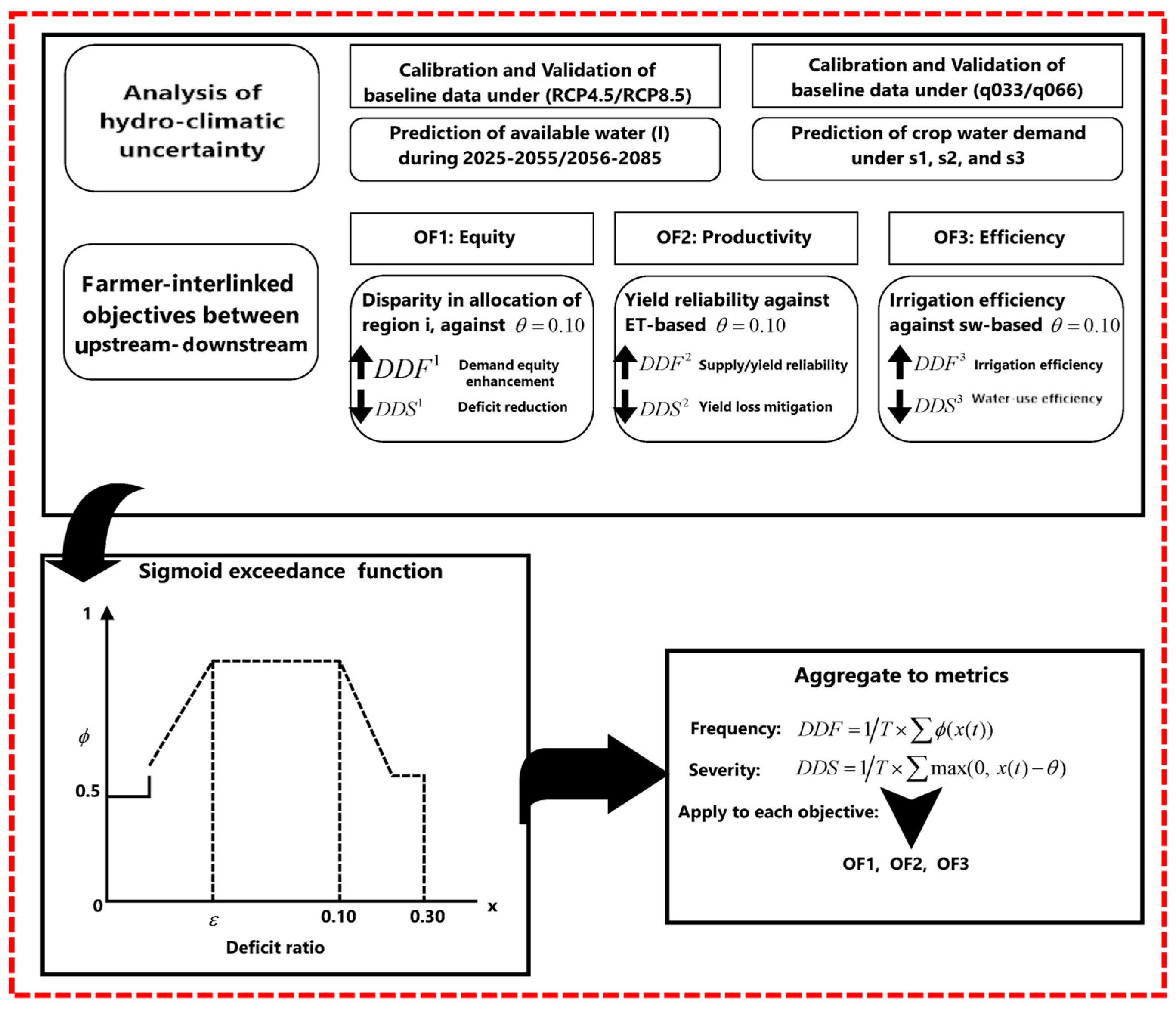
Upstream and downstream water demand reflects spatial differences in the availability of water resources and agricultural conditions. Upstream areas are prone to over-irrigation, waterlogging, and inefficiencies, whereas downstream regions often experience water scarcity, timing mismatches, and distribution conflicts [4,6]. Additionally, both regions also share common concerns, such as yield losses, irrigation timing, and operational inefficiencies [29]. In other words, upstream and downstream farmers often experience disparities in water access, raising concerns over irrigation reliability and crop yield stability [7]. Effective irrigation management in river basins requires balancing water distribution, crop productivity, and resource sustainability [18]. Sustainable solutions, including optimized water allocation, enhanced irrigation, and crop diversification, are essential to meet these challenges. Therefore, this study develops a novel SWAT-AquaCrop multi-objective framework to evaluate upstream and downstream demand deficits under quantile-based scenarios, addressing three key objectives: (1) Disparity Efficiency: ensuring equitable water distribution by minimizing allocation disparities between upstream and downstream areas, a major source of conflict and inefficiency; (2) Crop Yield Efficiency: maintaining stable crop production under available irrigation water, thereby sustaining agricultural productivity within water constraints; (3) Irrigation Efficiency: maximizing water use effectiveness by reducing losses and optimizing irrigation scheduling to improve overall irrigation efficiency and manage water shortages (Figure 1).

2.2. Framework for Investigating Frequency and Severity of Demand Deficit

This study evaluates system performance using three complementary objectives that capture inequitable allocation, crop yield losses, and irrigation delivery inefficiencies. Each objective is characterized through two indicators, demand deficit frequency ($DDF$) and demand deficit severity ($DDS$), representing the occurrence and magnitude of demand deficits. To ensure numerical stability, the binary exceedance operator is approximated with a smooth sigmoid function, avoiding discontinuities from indicator functions. This function provides a continuous measure of exceedance intensity while preserving the interpretation of deficit frequency:

$$\Phi (x;\theta ,\kappa )={\displaystyle \frac{1}{1+\exp [-\kappa (x-\theta )]}}$$

(1)

Here, $\theta$ represents the acceptable tolerance threshold, and $\kappa$ is a positive shape parameter controlling the sharpness of the transition from non-violation to violation.

OF1: Disparity in Water Allocation

The first objective function emphasizes equity by minimizing allocation disparities between upstream and downstream farmers, supporting sustainable and balanced water allocation [19,20]:

$$AD(i,t)=\left|{\displaystyle \frac{A_u(i,t)}{D_u(i,t)+D_d(i,t)}}-{\displaystyle \frac{A_d(i,t)}{D_u(i,t)+D_d(i,t)}}\right|$$

(2)

where $A_u(i,t)$ and $A_d(i,t)$ represent the total ratio of water allocated to the upstream and downstream areas $i$ at time $t$, and $D_u(i,t)$ and $D_d(i,t)$ refer to the total volume of water demand for upstream and downstream, respectively.

$$DD{F}^1(i)={\displaystyle \frac{1}{T}}{\displaystyle \sum _{t=1}^T{\displaystyle \sum _i\varphi (AD(i,t); {\theta }_1,k)}}, DD{S}^1(i)={\displaystyle \frac{1}{T}}{\displaystyle \sum _{i=1}^T\max (0,} AD(i,t)-{\theta }_1)$$

(3)

Indeed, ${DDF}^1$ measures how often the normalized allocation disparity between upstream and downstream farmers exceeds an acceptable tolerance level. It indicates the frequency of inequitable allocation events across the planning horizon. ${DDS}^1$ quantifies the magnitude by which allocation disparity surpasses the tolerance threshold, reflecting the intensity of inequity when it occurs.

OF2: Yield Deficit Due to Water Stress

The second objective seeks to minimize crop yield losses by linking productivity reductions directly to unmet crop water demand named $ET$ deficit [12]:

$$YDEF(i,t)=\left\{\begin{array}{ll}\min (1, {\displaystyle \frac{\max (0, E{T}_c(i,t)-E{T}_{act}(i,t)}{D(i,t)}}),& D(i,t)\rangle 0,\\ 0,& D(i,t)=0.\end{array}\right.$$

(4)

where $D (i,t)$ is water demand of region $i$ (upstream/downstream), ${ET}_c(i,t)$ refers to potential crop evapotranspiration (no stress), and ${ET}_{act}(i,t) denotes$ actual evapotranspiration (with stress).

$$DD{F}^2(i)={\displaystyle \frac{1}{T}}{\displaystyle \sum _{t=1}^T{\displaystyle \sum _i\varphi (YDEF(i,t);{\theta }_2,k)}}, DD{S}^2(i)={\displaystyle \frac{1}{T}}{\displaystyle \sum _{i=1}^T\max (0,}YDEF(i,t)-{\theta }_2)$$

(5)

${DDF}^2$ reflects the frequency of unmet crop water requirements, based on unmet evapotranspiration ($ET$) demand relative to total water demand, indicating periods of water stress Indeed, ${DDS}^2$ represents the extent to which ET-based yield deficit exceeds a specific tolerance threshold, providing a measure of the severity of crop water stress and associated potential yield reduction.

OF3: Irrigation Efficiency Deficit

The third objective aims to minimize operational inefficiency by evaluating the normalized shortfall between irrigation water demand and actual allocated water [21]:

$$S(i,t)={\displaystyle \frac{1}{T}}\left\{\begin{array}{ll}{\displaystyle \frac{\max (0, D(i,t)-A(i,t))}{D(i,t)}},& D(i,t)\rangle 0\\ 0& , D(i,t)=0\end{array}\right.$$

(6)

$$DD{F}^3(i)={\displaystyle \frac{1}{T}}{\displaystyle \sum _{t=1}^T{\displaystyle \sum _i\varphi (S(i,t);{\theta }_3,k)}}, DD{S}^3(i)={\displaystyle \frac{1}{T}}{\displaystyle \sum _{i=1}^T\max (0,}S(i,t)-{\theta }_3)$$

(7)

${DDF }^3$ indicates how often irrigation supply falls short of demand, and {$DDS$}³ quantifies the severity of these supply–demand mismatches.

In this study, a unified tolerance threshold was applied across all three objectives, with ${\theta }_1 = {\theta }_2 = {\theta }_3 = \theta = 0.10$. This threshold reflects a commonly accepted operational margin in irrigation systems, where deviations of up to 10% are typically tolerated due to conveyance losses, scheduling constraints, and measurement uncertainty. With all deficit indicators normalized, a single threshold allows consistent interpretation across equity, crop stress, and irrigation efficiency, eliminating subjective objective-specific tuning.

The parameter $\kappa$ controls the sharpness of the sigmoid transition and is set to 20 to closely approximate a binary threshold while maintaining numerical smoothness.

The rationale and numerical implications of these parameter choices are detailed in Section 2.2. The multi-objective optimization problem is subject to a set of physical and operational constraints to ensure that the solutions are feasible and realistic solutions.

Water Availability: The total agricultural water allocation cannot exceed the available water supply ($I\left(t\right)$) for each time period $t$:

$${\displaystyle \sum _i(A_u(i,t)+A_d(i,t))\le I(t) \forall t}$$

(8)

Allocation Bounds: These constraints define the practical and physical limits of how much water can be delivered to each region:

$$\begin{array}{l}{A}_u^{\min }(i,t)\le A_u(i,t)\le A_u^{\max }(i,t) \forall i,t\\ A_d^{\min }(i,t)\le A_d(i,t)\le A_d^{\max }(i,t) \forall i,t\end{array}$$

(9)

Minimum Water Requirement: This constraint ensures that the allocation is meaningful for agriculture. A common approach is to link allocation to the crop’s actual evapotranspiration ($ETc$) or water requirement ($D\left(t\right)$):

$$\begin{array}{l}{A}_u(i,t)\ge \alpha .D_u(i,t) \forall i,t\\ A_d(i,t)\ge \alpha .D_d(i,t) \forall i,t\end{array}$$

(10)

where $\alpha$ is a critical deficit factor ranging from 0 and 1. For instance, α = 0.5 requires the model allocate at least 50% of the full water requirement, preventing solutions that trivially resolve disparities by providing negligible water, which would severely reduce yields. In this study, $\alpha$ is considered as a scenario-dependen deficit factor, set to 0.8, 0.6, and 0.5 for scenarios $s_1$ (favorable), $s_2$ (normal), and $s_3$ (extreme), respectively. These values reflect realistic irrigation management responses under increasing water scarcity, where near-full irrigation is feasible in favorable years, moderate deficit irrigation is adopted under normal conditions, and only survival-level irrigation is possible during extreme droughts.

Non-negativity: All decision variables (water allocations) must be non-negative:

$$A_u(i,t)\ge 0, A_d(i,t)\ge 0 \forall i,t$$

(11)

The resulting formulation is a constrained, multi-objective nonlinear optimization problem. Due to the nonlinearity of the objective functions and the absence of explicit gradient information, the problem is solved using the Non-dominated Sorting Genetic Algorithm II (NSGA-II). The optimization formulation is implemented in MATLAB R2022b (MathWorks Inc., Natick, MA, USA) using a customized NSGA-II routine, with a population size of 100, 300 generations, a crossover probability of 0.9, and a mutation probability of 0.1. Convergence is assessed based on the stabilization of the Pareto front, and multiple independent runs ensure robustness and prevent premature convergence.

Uncertainty Representation and Parameter Sensitivity

To ensure robust representation of uncertainty and numerical stability in the optimization framework, key deficit identification parameters are explicitly justified and subjected to sensitivity analysis. The tolerance threshold $\theta$ represents the maximum acceptable deviation between irrigation water demand and allocated supply before a deficit event is considered operationally significant. In this study, $\theta$ is set to 0.10, corresponding to a 10% deviation. This value reflects commonly accepted operational margins in irrigation systems, accounting for conveyance losses, scheduling constraints, and measurement uncertainty. Since all deficit indicators are normalized, using a unified threshold ensures consistent interpretation across the three objectives: water allocation, crop water stress, and irrigation efficiency.

The parameter $\kappa$ controls the steepness of the sigmoid exceedance function approximate binary deficit events. $\kappa =20$ is selected to closely approximate a step function while preserving differentiability and numerical stability. Sensitivity tests were conducted for $\kappa$ values ranging from 10 to 30, confirming that the overall trends and relative ranking of optimal solutions are not sensitive to this parameter within the tested range, representing a balanced compromise between numerical smoothness and interpretability.

Overall, numerical sensitivity analysis is conducted for key model parameters regulating deficit identification and feasibility constraints. In particular, the sigmoid smoothness parameter $\kappa$ is varied within a plausible range (10–30), confirming that Pareto-front structure and solution ranking remain stable. Scenario-dependent specification of the critical deficit factor $\alpha$ further reflects adaptive management responses under varying water availability. Therefore, these components provide a structured and transparent treatment of dominant uncertainty sources relevant to basin-scale irrigation planning.

2.3. Implementation in SWAT-AquaCrop to Predict Initial Parameters

Using the SWAT-AquaCrop mechanism integrates the capabilities of both tools to predict key uncertain parameters like available water $\left(A\right)$ and crop yields $\left(Y\right)$. SWAT (Soil and Water Assessment Tool; Texas A&M University, College Station, TX, USA) is a hydrological model designed to simulate water movement, sediment transport, and nutrient dynamics in a watershed, making it suitable for assessing available water resources in both upstream and downstream regions.

Local-scale water availability is estimated with SWAT by incorporating projected climate impacts from General Circulation Models (GCMs) under RCP4.5 and RCP8.5 emission scenarios (RCP4.5 and RCP8.5) [14]. Next, because GSM outputs have coarse spatial resolution and are unreliable for capturing fine-scale hydrological patterns, a downscaling technique is applied to derive higher-resolution regional projections [15]. In this regard, this research applies Hadley Center Coupled Model (HadCM) as well as the Central European Climate Forecasting Center (ECMWF) with different emission SRES-scenario reports ($A_{1}B$, $B_1$, and $A_1$) to forecast upcoming streamflow patterns. Thus, to represent the spatial variability of the basin, the entire basin is divided into multiple sub-basins within the SWAT model. These sub-basins are further classified into Hydrological Response Units (HRUs) based on soil type, land use, topography (DEM), and slope classes. Finally, hydrological characteristics are predicted for each HRU to enhance the accuracy of the analysis. In addition, calibration and validation of the streamflow time series data are considered to evaluate the relative sensitivity of model outputs to parameter uncertainty. SWAT-CUP (Eawag, Dübendorf, Switzerland) is employed to calibrate parameters by minimizing discrepancies between simulated and observed data within the 95% PPU. Finally, SWAT-projected hydrological data are extracted for the RCP4.5 and RCP8.5 scenarios.

Accordingly, the SWAT model requires three key types of input data for the study area: topography, climate variables, and soil and land use characteristics. Precipitation and air temperature data are sourced from the ERA5 (European Centre for Medium-Range Weather Forecasts, Reading, UK) reanalysis dataset (ECMWF Fifth-Generation, (https://cds.climate.copernicus.eu (accessed on 15 December 2025)). These datasets are used to calibrate and validate the downscaled General Circulation Model (GCM) results for the period 2005–2020. Land use and soil maps are obtained from different sources: land use data at 300 m resolution are sourced from the Food and Agriculture Organization (FAO, Rome, Italy, https://www.fao.org/soils-portal), while soil data were obtained from SoilGrids (ISRIC—World Soil Information, Wageningen, The Netherlands, https://lpdaac.usgs.gov/products/mod16a2v006 (accessed on 15 December 2025). The digital elevation model (DEM; NASA, Washington, DC, USA) at resolution 30 m was obtained from the Shuttle Radar Topography Mission (SRTM; NASA, Washington, DC, USA; https://lpdaac.usgs.gov/products/srtmgl1v003/, accessed on 15 December 2025). Also, the evapotranspiration rate beyond some other technical specification data is obtained from the MODIS Global Evapotranspiration (MOD16; NASA, Washington, DC, USA) (https://lpdaac.usgs.gov/products/mod16a2v006 (accessed on 15 December 2025).

Furthermore, this research employs AquaCrop (Food and Agriculture Organization of the United Nations, Rome, Italy) to simulate yield responses for selected crops in the study area. To run AquaCrop, several datasets need to be considered including climate data, soil data, crop data, and management practices. Soil moisture, evapotranspiration, and precipitation data are extracted from SWAT model outputs. Indeed, basin-scale hydrological outputs from SWAT, including effective precipitation, soil moisture status, and water availability constraints, are used to parameterize irrigation water supply and soil water conditions in AquaCrop. The analysis focuses on wheat and maize, using high-resolution cropping intensity maps from the Global Yield Gap Atlas (https://www.yieldgap.org (accessed on 15 December 2025), complemented by farmer-reported yield data for calibration.

To configure AquaCrop for wheat and maize yield simulation, crop-specific parameters are defined, including growing degree days (GDD), canopy development dynamics, transpiration efficiency, and crop water productivity. The water productivity parameter is specified for each crop within the typical range of 10–15 g biomass per kg of water transpired. Climate inputs, including daily precipitation, minimum and maximum temperature, solar radiation, relative humidity, and wind speed, are used to drive crop growth and evapotranspiration processes.

Soil physical properties such as texture, field capacity, wilting point, and hydraulic conductivity are parameterized based on basin-specific data. Irrigation management scenarios (T0–T10) are subsequently defined to represent both rainfed and irrigated conditions. These scenarios differ in their irrigation triggering strategies, which are based either on predefined crop growth stages or on automatic soil moisture threshold criteria. Crop management practices, including planting method, fertilization level, and field conditions, are specified accordingly. Finally, the model is calibrated and validated by adjusting crop coefficients to align simulated yields and water use with observed data.

2.4. Scenario Construction from SWAT–AquaCrop Outputs

To represent hydro-climatic variability within the optimization framework, three distinct scenarios are derived directly from the SWAT–AquaCrop modeling chain. SWAT is used to simulate seasonal water availability ($A\left(t\right)$) in the upstream and downstream sub-basins, while AquaCrop estimated the corresponding seasonal crop water requirements ($D\left(t\right)$) for wheat and maize. For each period t, the deficit ratio ($DR\left(t\right)$) is defined to quantify the fraction of crop water demand that remains unmet as:

$$DR(t)={\displaystyle \frac{\max (0, D(t)-A(t))}{D(t)}} t=1,2,\dots ,T$$

(12)

$D(t)={\displaystyle {\sum }_{j,i}{D}_{j,i}(t)}$ is the total basin crop water demand aggregated over crop $j$ and region $i$ (upstream and downstream), and $A\left(t\right)$ is the basin water allocation from SWAT-simulated supply at time $t$. The time index $t$ represents a discrete crop growing season, during which SWAT-simulated water availability and AquaCrop-derived crop water demand are aggregated consistently with the basin-scale irrigation planning horizon used in the optimization. By definition, $DR\left(t\right)=0$ indicates full satisfaction of crop demand, whereas values approaching 1 correspond to extreme deficit conditions.

Daily crop evapotranspiration ($ETc$) is computed in AquaCrop as:

$$ET{c}_{j,i}(t)=K_{c,j}(t)\times ET{o}_i(t)$$

(13)

where $K_{c, j}\left(t\right)$ denotes the stage-specific crop coefficient (initial, development, mid-season, and late-season) for wheat or maize, and ${ETo}_i\left(t\right)$ represents the reference evapotranspiration, derived from the SWAT meteorological inputs using the FAO-56 Penman–Monteith formulation. Daily crop water demand is defined as $D_{j,i}(t)=\max (0, ET{c}_{j,i}(t)-P_i^{eff}(t))$, where $P_i^{eff}(t)$ represents effective precipitation, the portion of rainfall available for crops after runoff and deep percolation, and is obtained directly from SWAT outputs rather than empirical estimates.

However, hydro-climatic uncertainty is represented using a quantile-based scenario classification approach, whereby historical rainfall and runoff distributions are partitioned into discrete percentile-based scenarios. Percentile thresholds are selected to capture distinct hydrological regimes while ensuring sufficient sample size within each scenario for statistical robustness. Specifically, lower quantiles represent dry and stress-prone conditions, middle quantiles correspond to near-normal conditions, and upper quantiles reflect wet or surplus conditions. This approach avoids assumptions about the underlying distribution and preserves the empirical variability of the hydro-climatic record.

However, percentile-based classification is preferred because it provides a transparent, non-parametric, and reproducible representation of uncertainty, while retaining direct interpretability for irrigation decision-making. Moreover, quantile-based scenarios have been widely adopted in water allocation studies to balance model complexity with practical applicability under limited data conditions.

3. Case Study

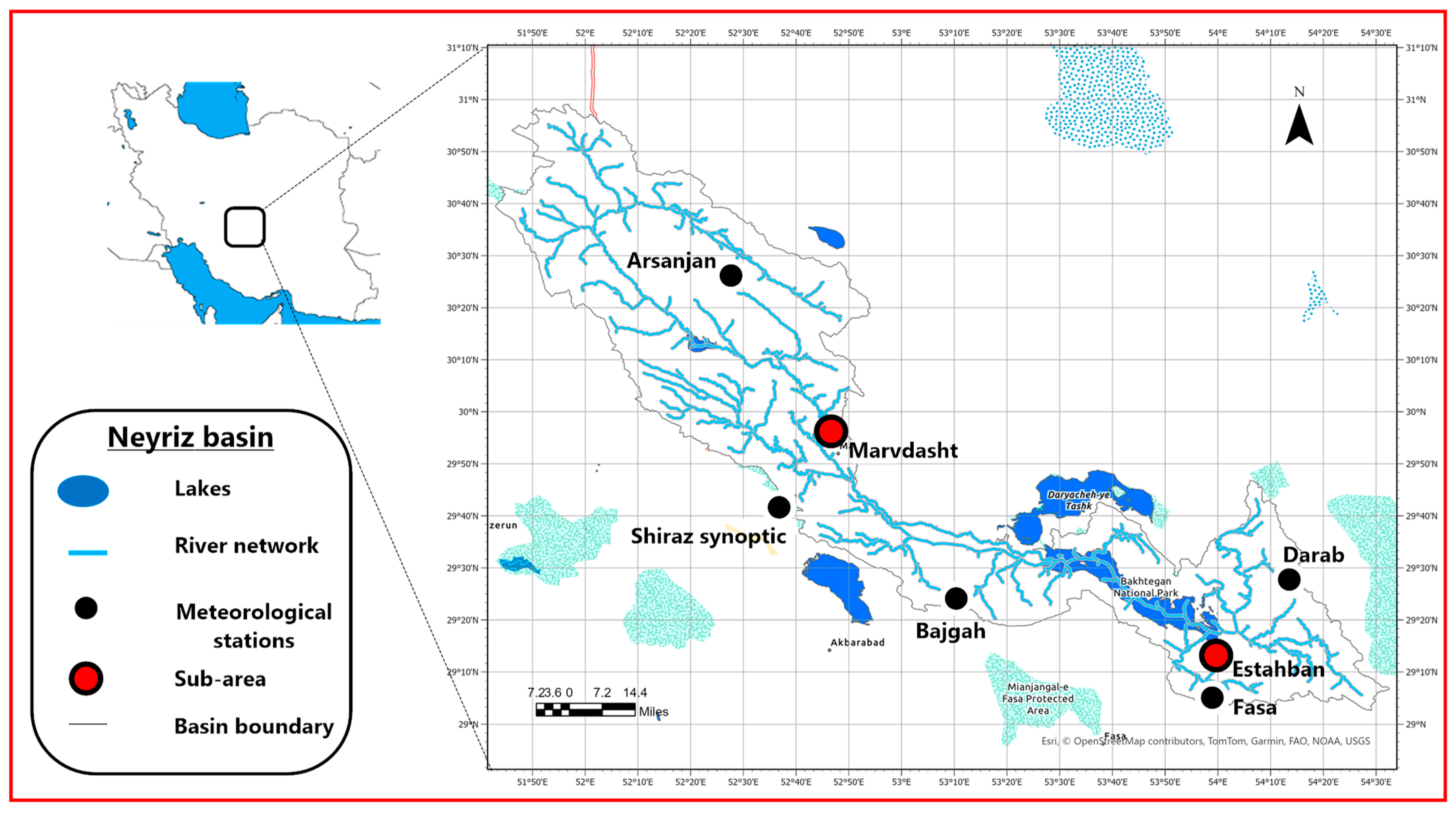
The Neyriz Basin (29°11′39.62″ N to 54°19′11.60″ E) in Fars Province, Iran, is an arid agricultural region hydrologically dominated by the Kor River, which sustains irrigation and feeds the saline lakes of the basin, including Lake Bakhtegan and Lake Tashk [16]. Farmers in Marvdasht (upstream) and Estahban near Bakhtegan Lake (downstream) rely on the Kor River for irrigation (Figure 2), particularly for water-intensive crops such as wheat and maize [23,30,31]. However, extensive water withdrawals for multiple uses diminish the river’s flow, causing irrigation shortages for farmers in both Marvdasht and Estahban and exacerbating regional disparities [32,33]. This disparity challenge has resulted in declining wheat and maize yields, increased reliance on groundwater, and heightened economic vulnerability for farmers [34]. Moreover, climate variability, inefficient water management, and competition for resources further intensify these challenges [35].

Overall, the frequency and severity of demand deficit in both upstream and downstream areas reflects the growing water crisis in the Neyriz Basin. Farmers report concerns regarding future water availability, irrigation efficiency, risk of crop failure, and financial instability. Addressing these challenges requires sustainable water management strategies, equitable allocation policies, and alternative cropping systems to reduce reliance on water-intensive cultivation.

Accordingly, the key parameters of the study area required for the simulation process are summarized in

Table 1. Land use classification in Neyriz watershed.

No.	SWAT Code	Description	Area (%)
1	WATR	Water, Pond	8
2	URMD	Urban Medium Density	3
3	WETN	Emergent/Herbaceous Wetlands	7
4	AGRL	Cropland and Pasture	17
5	RNGB	Shrub and Brush Rangeland	21
6	RNGE	Mixed Rangeland	13
7	SWRN	Bare Ground	31

,

Table 2. Sensitive parameter ranges for calibration.

Model Parameter	Definition	L/U	Calibrated Interval	p-Value
v_SURLAG	Surface runoff lag coefficient	0.00 to 12.00	2.50	0.00
r_RCHRG_DP	Deep aquifer percolation fraction	0.00 to 1.00	0.45	0.03
v_GWQMN	Threshold depth of water in shallow aquifer required for return flow	1500 to 5000	2200	0.05
r_CN2	SCS runoff curve number for moisture condition II.	−0.30 to 0.30	−0.22	0.00
v_ALPHA_BF	Base flow alpha factor	0.40 to 1.00	0.63	0.00
v_ CH_K2.rte	Channel hydraulic conductivity	−0.50 to 0.50	0.32	0.15
r_Sol_ AWC	Soil available water capacity	−0.20 to 0.20	0.12	0.00
v_EPCO	Plant update compensation factor	[−1, 1]	0.78	0.08

Note(s): v means that the parameter needs to be replaced by a given value; r means that the parameter value needs to be multiplied by (1 + a given value). Groundwater-related parameters are calibrated internally within SWAT to properly simulate recharge and baseflow but fall outside the direct focus of this study’s analysis.

and

Table 3. Parameters employed for model calibration in AquaCrop.

Parameters	Marvdasht		Estahban
	Wheat	Maize	Wheat	Maize
Time from sowing to senescence (days)	130	120	125	115
Maximum effective rooting depth (cm)	120	150	110	140
Time from sowing to emergence (days)	10	7	11	8
Maximum canopy cover (%)	90	98	85	95
Time from sowing to max canopy cover (days)	55	45	50	42
Length of flowering period (days)	15	18	14	17
Time from sowing to physiological maturity (days)	120	110	115	105
Time from sowing to maximum root depth development (days)	70	60	65	55
Initial canopy cover (%)	10	12	10	12
Time from sowing to flowering (days)	70	50	65	48

:

Although several calibrated parameters in Table 2 are related to groundwater processes (deep aquifer percolation and shallow aquifer thresholds), groundwater dynamics are not analyzed explicitly in this study. These parameters are calibrated as part of the internal SWAT water balance to ensure realistic simulation of streamflow and soil–plant water availability. The analysis focuses on surface water availability, crop water demand, and irrigation-related deficits, rather than on groundwater abstraction or allocation.

4. Results and Analysis

4.1. Investigation of Downscaling Validation

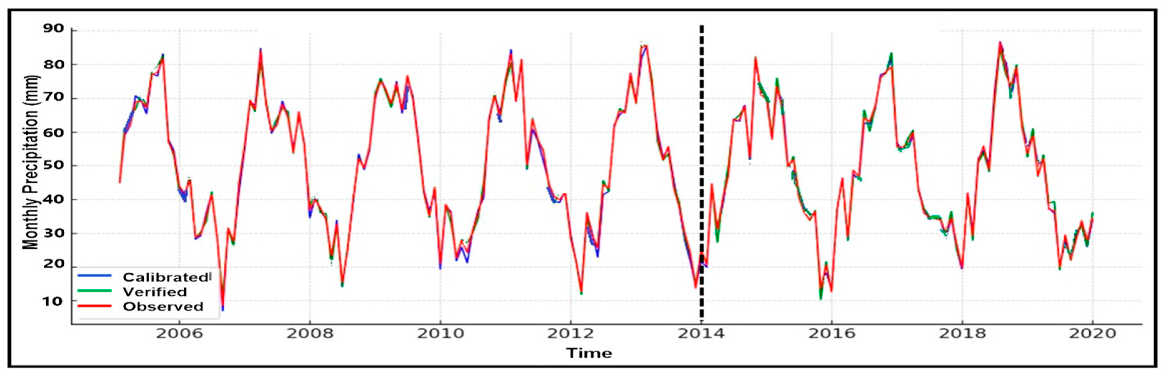
The initial phase of the calibration and validation process involved identifying the most sensitive parameters and evaluating their accuracy within the study basin. In this context, the SCS-CN method was employed to estimate monthly precipitation, identified as the most influential parameter. Considering the basin’s distinct characteristics, including its slope, eight sensitive parameters with varying degrees of influence were established to evaluate inflow rates. For the downscaling process, the model was calibrated using data from the 2005–2014 period (10 years) and validated over the 2015–2020 period (6 years). During the calibration period, the $P-factor$, representing the percentage of observed data bracketed by the 95PPU, ranged between 0.72 and 0.84, while the $R-factor$, indicating the average thickness of the 95PPU band relative to the standard deviation of observed data, varied between 0.85 and 1.2 across the six stations. These results indicate that the model simulations remained within acceptable uncertainty bounds. During the validation period, the $P-factor$ slightly declined to 0.65–0.78, while the $R-factor$ remained below 1.3, indicating a reasonable trade-off between model accuracy and uncertainty. The spatial variation in these metrics reflects local hydrological variability across different sub-basins (Figure 3).

Furthermore, statistical metrics, including the coefficient of determination ($R^2$), Nash–Sutcliffe efficiency ($NSE$), Nash–Sutcliffe coefficient ${NSE}_{rel}$, and root mean square error ($RMSE$), were analyzed at five stations to assess the model’s performance within the studied basin. $R^2$ and $NSE$ serve as key indicators of model performance, with the $R^2$ values exceeding 0.5 indicating acceptable fit and reduced variance error. In general, these metrics confirm a satisfactory level of consistency between the observed and simulated data (

Table 4. Statistical metrics for precipitation downscaling during calibration (2005–2014) and validation (2015–2020); $R^2$ > 0.5, $NSE > 0.5$, and $RSR < 0.7$ indicate satisfactory model performance.

Station	${\mathit{R}}^2$	$\mathit{N}\mathit{S}\mathit{E}$	${\mathit{N}\mathit{S}\mathit{E}}_{\mathit{r}\mathit{e}\mathit{l}}$	$\mathit{R}\mathit{S}\mathit{R}$
	Cal/Val	Cal/Val	Cal/Val	Cal/Val
Shiraz Synoptic	0.76/0.59	0.79/0.61	0.77/0.68	0.48/0.51
Darab	0.51/0.74	0.48/0.76	0.73/0.82	0.53/0.59
Arsanjan	0.79/0.70	0.78/0.64	0.79/0.74	0.42/0.56
Bajgah	0.54/0.59	0.84/0.89	0.68/0.75	0.55/0.49
Fasa	0.81/0.73	0.75/0.70	0.67/0.72	0.37/0.45

).

The calibration and validation results indicate that the SWAT model reliably represents the basin’s hydrological behavior under both historical and future climate scenarios. The $P-factor$ and $R-factor$ values indicate that simulated streamflow fell within acceptable uncertainty bounds, while the statistical metrics ($R^2$ and $NSE$) confirmed that the model captures both seasonal patterns and inter-annual variability across sub-basins. These results provide confidence in the SWAT-derived water-availability projections used to drive the subsequent AquaCrop simulations and multi-objective optimization. Accordingly, the optimization results, directly driven by these hydrological inputs, provide a robust basis for assessing irrigation-deficit frequency and severity under hydro-climatic uncertainty.

As presented in

Table 5. Modifications in rainfall and temperature patterns under different greenhouse gas emission scenarios.

Sub-Basin	Precipitation (%)				Temperature (°C)
	RCP 4.5 [2025–2055]	RCP 4.5 [2056–2085]	RCP 8.5 [2025–2055]	RCP 8.5 [2056–2085]	RCP 4.5 [2025–2055]	RCP 4.5 [2056–2085]	RCP 8.5 [2025–2055]	RCP 8.5 [2056–2085]
Bakhtegan	+3	0	−1	−3	+2	+2	+2	+4
Maharloo	+5	+2	+1	−4	+1	+3	+3	+5
Marvdasht	+4	+4	−2	0	0	+1	0	+1
Estahban	+1	−2	−3	−5	+2	0	+1	+3

, the projected changes in precipitation and temperature across key sub-basins under RCP4.5 and RCP8.5 scenarios indicate a general decline in rainfall and a consistent rise in temperature between the 2025–2055 and 2056–2085 periods. For instance, under RCP8.5, Estahban was projected to experience a precipitation reduction from −3% to −5%, alongside a temperature rise from +1 °C to +3 °C.

In general, Table 5 highlights consistent hydro-climatic trends across the Neyriz sub-basins under both RCP4.5 and RCP8.5 scenarios. Temperature shows a robust, monotonic increase across all sub-basins and time horizons, with stronger warming under RCP8.5, whereas precipitation responses were more spatially heterogeneous, exhibiting both moderate increases and declines depending on sub-basin and period. These contrasting patterns indicate that future irrigation stress is likely to be driven primarily by rising evaporative demand rather than by uniform changes in rainfall.

4.2. Calibration and Validation of Crop Yield Using Aquacrop

Accurate simulation of crop phenology and yield response is critical, as $ET$-based unmet demand directly emphasizes the yield-related demand deficit frequency (${DDF}^2$) and severity (${DDS}^2$). The model was calibrated using the crop-specific parameters listed in Table 3 and validated against observed yield data from 2005 to 2020. Statistical performance indicators, including the coefficient of determination ($R^2$), Nash–Sutcliffe efficiency ($NSE$), and root mean square error ($RMSE$), were calculated for both calibration (2005–2014) and validation (2015–2020) periods (

Table 6. Statistical performance indicators for AquaCrop yield calibration and validation.

Crop	Sub-Area	Period	${\mathit{R}}^2$	$\mathit{N}\mathit{S}\mathit{E}$	$\mathit{R}\mathit{M}\mathit{S}\mathit{E}(\mathbf{t}/\mathbf{h}\mathbf{a})$
Wheat	Marvdasht	Cal/	0.85	0.82	0.42
		Val	0.81	0.78	0.44
	Estahban	Cal/	0.82	0.79	0.40
		Val	0.78	0.74	0.45
Maze	Marvdasht	Cal/	0.80	0.77	0.52
		Val	0.76	0.72	0.55
	Estahban	Cal/	0.78	0.75	0.50
		Val	0.72	0.68	0.58

). The results indicate high agreement between simulated and observed yields for all crop–region combinations. During calibration, $R^2$ exceeded 0.78 and $NSE$ exceeded 0.75, while validation performance remained strong ($R^2\ge 0.72$; $NSE$ ≥ 0.68), with $RMSE$ values below 0.58 t/ha.

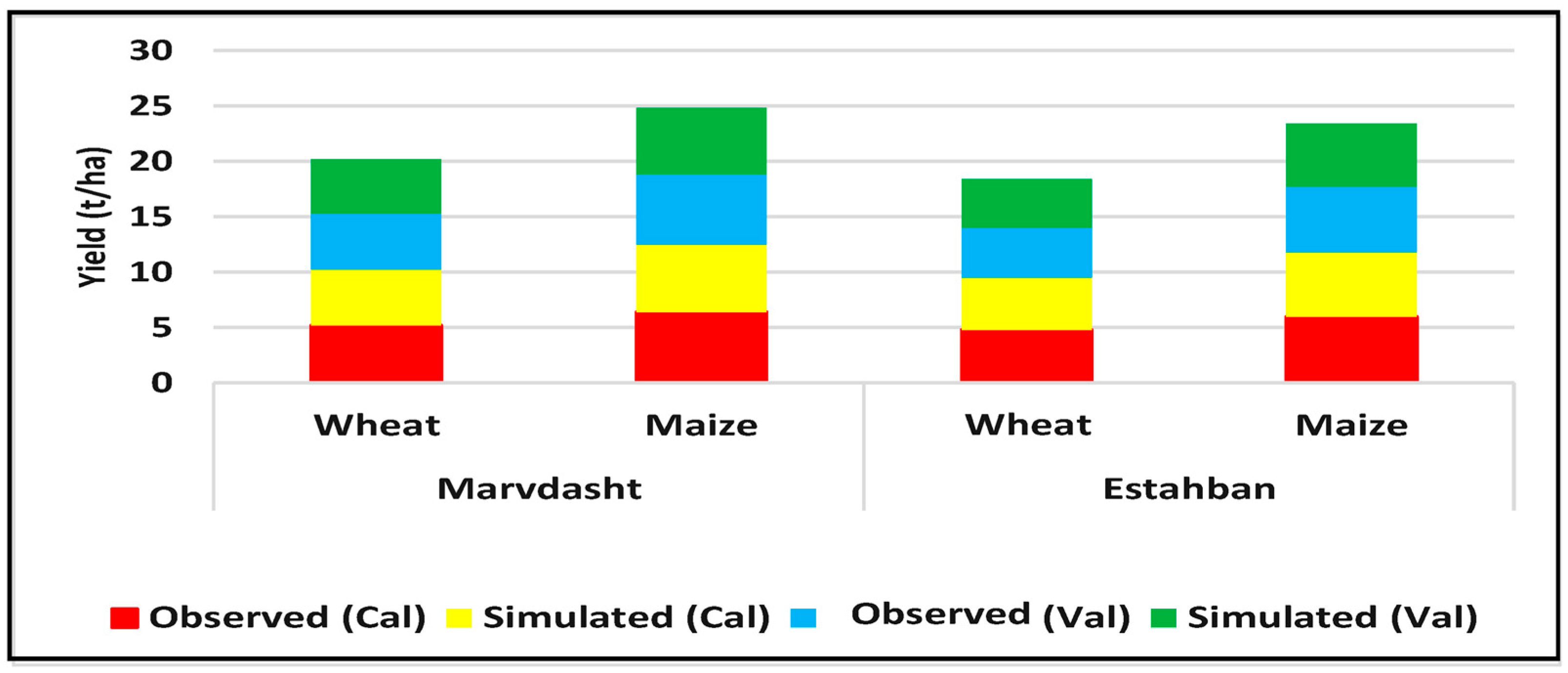
The calibration process was further refined by incorporating crop-specific parameters, including phenological stages and rooting depth, thereby improving the agreement between model predictions and observed data. These adjustments were applied iteratively to the selected crops to ensure that the model accurately represented the agro-climate status of the study area. The close alignment between observed and modeled values demonstrates the reliability of AquaCrop for yield prediction under local agro-climatic conditions (Figure 4). Furthermore, the calibrated crop parameters ensure that simulated potential evapotranspiration (${ET}_c$), used to quantify unmet water demand in the yield deficit objective ($YDEF$), accurately reflects local growing conditions. This establishes a direct link between calibrated crop responses and the $ET$-based demand deficit metrics (${DDF}_2$ and ${DDS}_2$) that drive the optimization of irrigation allocation and scheduling.

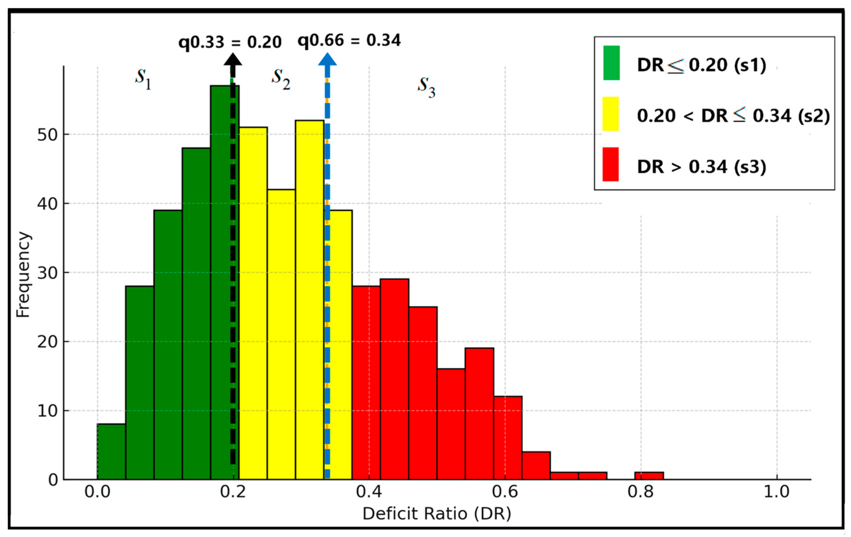
Based on the empirical distribution of $DR\left(t\right)$ across the baseline (2005–2020) and projected periods (RCP4.5 and RCP8.5), three representative scenarios were classified using quantile thresholds. Specifically, the 33rd ($q0.33$) and 66th ($q0.66$) percentiles of the $DR\left(t\right)$ distribution were used to define three equally probable, non-parametric scenarios:

s₁ (Favorable): $DR\left(t\right)\le q0.33$, representing years with low or negligible deficit (ample water supply relative to demand).

s₂ (Normal): q0.33 < DR(t) ≤ q0.66, representing years with moderate supply–demand balance and typical irrigation stress.

s₃ (Extreme): DR(t) > q0.66, representing years with severe water shortages and high unmet demand.

The separation of irrigation performance across scenarios confirms that the quantile-based classification effectively distinguishes hydrologically favorable, normal, and stress conditions. The consistency of observed trends across scenarios indicates that the optimization results are not artifacts of arbitrary threshold selection but instead reflect systematic responses to progressively increasing hydro-climatic stress. The thresholds $q0.33$ and $q0.66$ represent the 33rd and 66th percentiles of the deficit ratio distribution $DR\left(t\right),$ derived empirically from SWAT–AquaCrop outputs. This non-parametric classification divides the time series into three equally probable categories (favorable, normal, and extreme), ensuring that scenario definitions are data-driven and unbiased by parametric assumptions.

Figure 5 illustrates the empirical distribution of the deficit ratio ($DR$), derived from the SWAT–AquaCrop simulation over the baseline and projected periods. The histogram was partitioned into three quantile-based categories: favorable ($s_1$, $DR$ ≤ 0.20), normal ($s_2$, 0.20 < $DR$ ≤ 0.34), and extreme ($s_3$, $DR$ > 0.34). This non-parametric classification ensures that scenario thresholds were data-driven, reflecting the underlying variability of supply–demand imbalances rather than arbitrary assumptions. The dominance of normal conditions indicates that moderate irrigation stress was the most recurrent state in the Neyriz Basin, while the occurrence of extreme deficit, although less frequent, represents critical risk years for both upstream and downstream farmers. By grounding scenario construction in the observed $DR$ distribution, the framework provides a robust basis for analyzing water allocation strategies under diverse hydro-climatic conditions.

4.3. Yield and Water Productivity Under Irrigation Scenarios

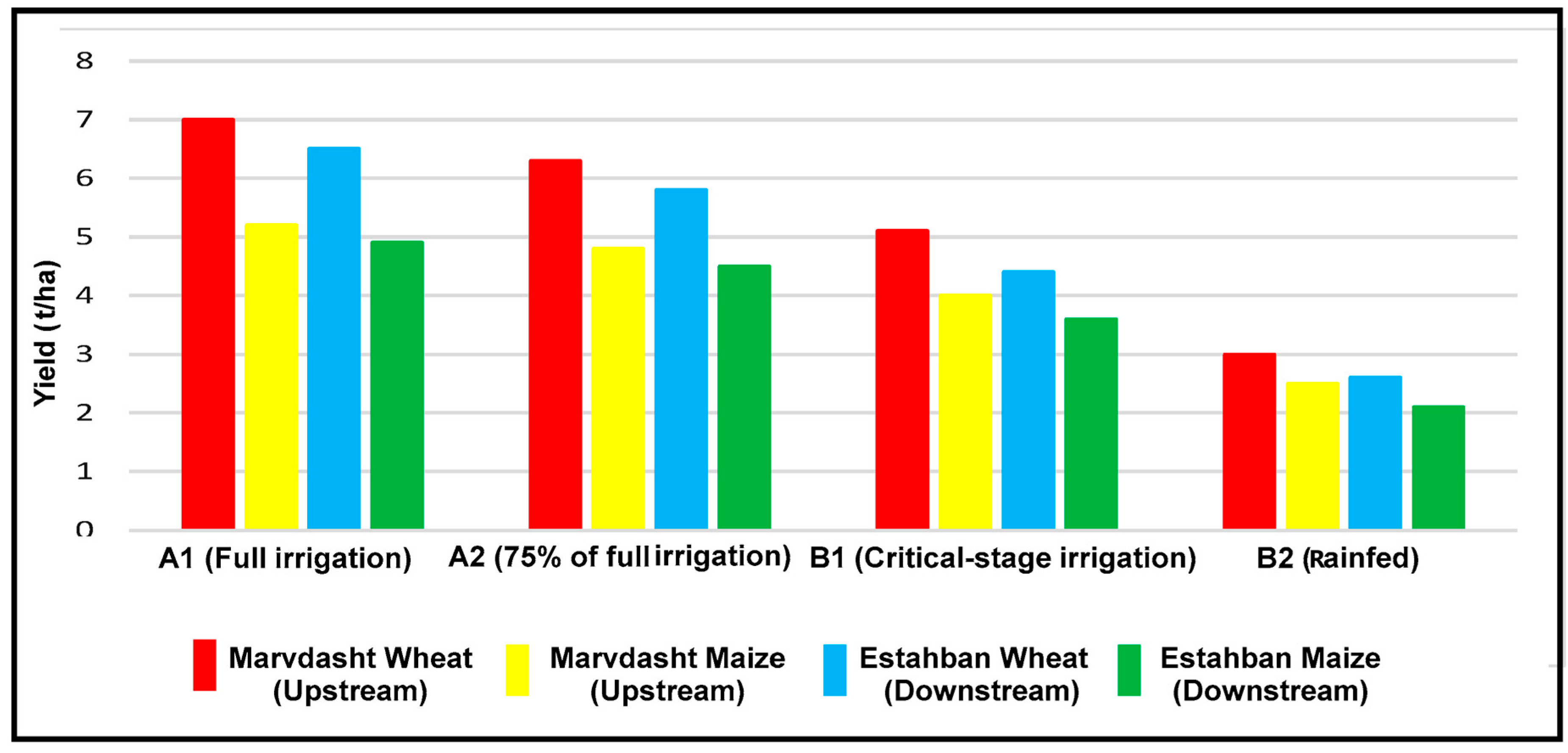
Figure 6 presents simulated yield responses under four irrigation scenarios: A1 (full irrigation), A2 (75% $ETc$ replacement), B1 (irrigation at critical growth stages only), and B2 (rainfed). As expected, crop yields declined with increasing irrigation stress, from 5.2 t/ha (A1) to 2.5 t/ha (under B2) for wheat and from 7.0 t/ha to 3.0 t/ha for maize in Marvdasht (upstream). In the downstream Estahban region, yield reductions were more pronounced due to higher atmospheric evaporative demand and lower effective rainfall, confirming the greater vulnerability of downstream agriculture to irrigation deficit. Notably, the B1 strategy retained approximately 72–78% of full-irrigation yields for both crops in both regions, indicating the efficiency of stage-targeted irrigation in conserving water while maintaining yield productivity.

From a demand deficit perspective, observed yield reductions correspond to higher frequencies of unmet crop water requirements during sensitive phenological stages. Specifically, scenarios A2 and B2, which exhibited larger yield gaps, inherently show higher demand deficit frequency (${DDF}^2$) and severity (${DDS}^2$) due to more frequent and intense evapotranspiration shortfalls, particularly during water-sensitive stages such as flowering and grain-filling. In contrast, the B1 strategy, which maintained 72–78% of full-irrigation yields with reduced water input, indicates that irrigation timing aligned with critical growth stages can substantially reduce ${DDF}^2$ and ${DDS}^2$. These results confirm that the $ET$-based deficit metrics used in the optimization framework accurately capture the agronomic reality: yield losses are determined not only by total seasonal water shortage but also by how often and how severely crop water requirements are unmet during pivotal phenological windows.

4.4. Optimal Outputs Under Quantile-Based Scenarios

Table 7. Optimized frequency of demand deficit frequency and severity ($DFF \& DDS$, %) under different scenarios.

Crop	Scenario	Marvdasht Baseline/Optimized			Estahban Baseline/Optimized
		DDF1 DDS1	DDF2 DDS2	DDF3 DDS3	DDF1 DDS1	DDF2 DDS2	DDF3 DDS3
Wheat	S1	15.2/9.1	12.8/7.5	10.6/6.2	17.0/10.4	14.3/8.9	11.5/7.3
		20.0/12.0	17.1/10.0	14.9/9.7	26.2/16.7	23.5/14.2	21.8/13.9
	S2	22.4/14.3	18.9/11.2	15.7/9.6	24.6/16.2	20.7/13.4	17.8/10.8
		32.9/21.0	28.3/18.1	25.5/16.7	41.6/27.0	34.8/23.2	32.0/20.9
	S3	31.7/21.5	27.8/18.6	23.5/15.2	34.2/23.7	29.5/20.3	25.6/16.7
		46.4/31.8	40.0/27.3	35.7/24.6	54.3/36.8	47.7/31.4	44.2/30.7
Maize	S1	16.4/9.7	13.6/8.1	11.2/6.8	18.2/11.0	15.1/9.5	12.1/7.9
		21.8/14.2	19.5/12.3	17.4/11.0	28.0/17.7	25.6/16.2	23.8/15.3
	S2	23.9/15.1	19.8/12.4	16.5/10.2	25.8/16.8	21.9/14.0	18.3/11.7
		36.2/24.8	30.0/20.2	27.5/18.9	43.0/28.9	37.0/24.5	34.1/23.3
	S3	33.0/22.6	28.7/19.2	24.8/15.9	35.5/24.1	30.9/21.4	26.9/17.4
		49.9/33.0	43.5/29.3	39.1/26.3	58.7/40.0	50.6/35.2	47.2/33.0

shows that optimization consistently reduces demand deficit frequency and severity ($DDF$&$DDS$) across all scenarios, with the largest improvements observed under extreme deficit conditions ($s_3$). For example, in downstream Estahban, the allocation-disparity deficit frequency (${DDF}^1$) for maize declined from 35.5% under baseline conditions to 24.1% after optimization, representing an 11.4 percentage reduction. Across all scenarios, improvements were systematically larger for downstream users and for maize relative to wheat, reflecting higher baseline vulnerability to water shortages.

Under extreme conditions ($s_3$), the yield-related deficit severity (${DDS}^2$) for maize in Estahban decreased from 43.5% to 29.3%, corresponding to an approximate 33% reduction, indicating that deficit events, when they occur, are considerably less intense. For wheat in the same region, irrigation efficiency deficit severity (${DDS}^3$) decreased from 44.2% to 30.7% under $s_3$ conditions, corresponding to a reduction exceeding 30%. These consistent reductions in $DDS$ across crops, regions, and objectives underscore the effectiveness of the proposed framework in mitigating both the frequency and magnitude of irrigation demand deficits under severe hydro-climatic stress.

Although Table 7 presents a detailed set of scenario-based outcomes, several consistent patterns are evident. First, improvements in both deficit frequency ($DDF$) and severity ($DDS$) are systematically greater for downstream users (Estahban) compared to upstream areas (Marvdasht), reflecting a targeted correction of baseline inequities. Second, reductions in deficit severity ($DDS$) are generally more pronounced than reductions in deficit frequency ($DDF$), indicating that the optimization framework is particularly effective in mitigating extreme shortages rather than eliminating deficits entirely. Third, the magnitude of improvement is greatest under the extreme deficit scenario ($s_3$), where all objectives show their strongest response. In general, these results highlight that the framework delivers its most substantial benefits under high-stress conditions, particularly for downstream and water-vulnerable users.

Table 4, Table 5, Table 6 and Table 7 summarize the optimized irrigation allocation outcomes across different hydro-climatic scenarios. The results show a systematic redistribution of irrigation water between upstream and downstream regions compared to baseline allocation conditions. Under dry and normal scenarios, the optimization framework reduces downstream irrigation deficits by moderately adjusting upstream withdrawals, thereby enhancing allocation equity while maintaining overall irrigation efficiency.

Under wet scenarios, increased water availability allows both regions to achieve higher allocation satisfaction, resulting in reduced deficit frequency and severity and improved crop water adequacy.

In particular, the results indicate that relatively small reductions in upstream allocations can generate disproportionately larger benefits in downstream deficit mitigation, underscoring the potential of coordinated, basin-scale optimization to alleviate persistent upstream–downstream irrigation conflicts.

4.5. Irrigation Schedule Adjustments and Allocation Patterns

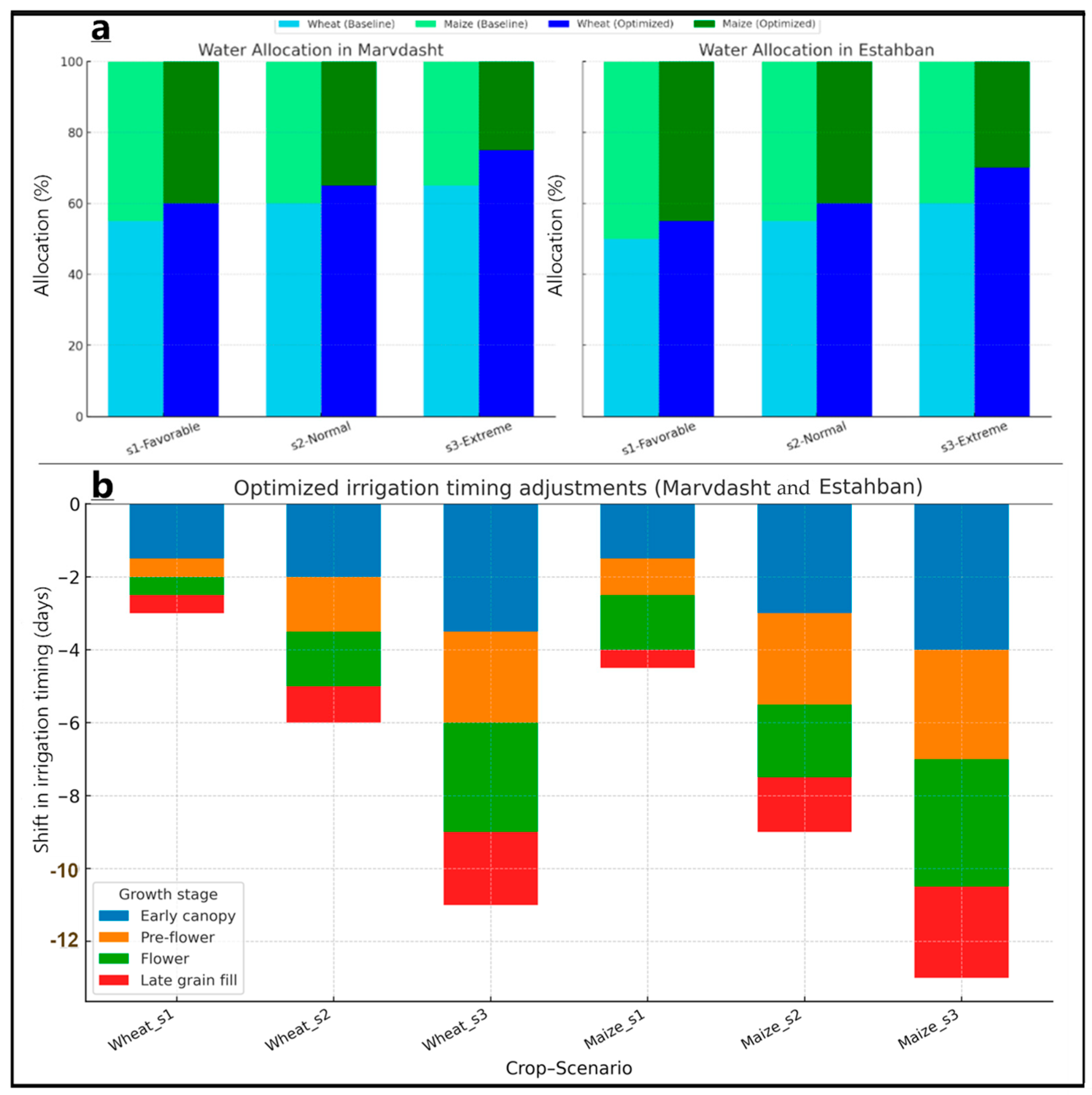
Figure 7a,b depict how the optimization framework converts deficit-minimization objectives into coordinated water allocation strategies and stage-specific irrigation schedules. Water allocation percentages (%) represent the proportion of total available irrigation water assigned to each treatment, not the fraction of crop demand. Figure 7a shows that optimized allocation substantially reduced disparities between upstream Marvdasht and downstream Estahban, particularly under the extreme scenario ($s_3$). While baseline allocation disproportionately favored upstream farmers, the optimized schedule redistributed water more equitably across both regions, thereby reducing the frequency and severity of disparity-related deficits. Figure 7b further highlights how these allocations were implemented through stage-specific irrigation timing adjustments. Across scenarios, irrigation events were consistently shifted earlier relative to the baseline (25, 50, 75, and 100 days after sowing ($DAS$), with the largest advances observed during flowering and grain-filling stages. These shifts are more pronounced in downstream Estahban and under severe deficit conditions, reaching 4–5 days in ${ s}_3$, reflecting both heightened crop sensitivity during reproductive stages and increased downstream vulnerability to supply shortfalls.

The integrated behavior observed across Figure 5, Figure 6 and Figure 7 highlights the importance of coupling hydrological, crop, and optimization models when addressing irrigation allocation under uncertainty. By explicitly linking hydro-climatic variability to crop water stress and allocation outcomes, the framework moves beyond static or sector-isolated optimization approaches. This integration is critical in upstream–downstream systems, where localized allocation decisions can influence basin-scale equity and irrigation efficiency.

Compared to conventional allocation methods that rely on fixed priorities or single-objective optimization, the proposed framework enables adaptive trade-off analysis across equity, productivity, and irrigation efficiency objectives. The results emphasize that system-wide performance gains can be achieved through coordinated adjustments rather than strict prioritization, offering a practical pathway for improving irrigation management under increasing hydro-climatic variability.

4.6. Discussion

The integration of SWAT and AquaCrop within a multi-objective optimization framework provides new insights into basin-scale irrigation management under hydro-climatic uncertainty. The scenario-based results depict pronounced upstream–downstream asymmetries in deficit frequency and severity, driven by contrasting hydrological availability and crop water requirements. Accordingly, downstream farmers experience systematically higher baseline deficits across equity, yield, and irrigation efficiency objectives, underscoring the structural nature of allocation inequity in river basins.

A key finding is the strong dependence of optimization benefits on hydro-climatic conditions. Under favorable scenarios, performance improvements are relatively modest, whereas under extreme deficit conditions the framework substantially reduces both deficit frequency and severity. This indicates that the proposed approach is particularly effective during stress periods, when targeted allocation and scheduling adjustments can significantly mitigate downstream vulnerability and reduce inequity.

Specifically, the results demonstrate that equity and productivity gains are not mutually exclusive. By simultaneously optimizing disparity efficiency, yield efficiency, and irrigation efficiency, the framework mitigates the trade-offs commonly reported in single-objective or priority-based allocation schemes. This finding has direct policy relevance, indicating that equitable water reallocation can be achieved without compromising agricultural productivity when decisions are informed by integrated hydrological and crop-system dynamics.

From an implementation perspective, the framework is tractable for basin authorities. It relies on hydrological and agricultural outputs that are typically available through meteorological services, remote-sensing products, and agricultural statistics. The use of quantile-based scenarios offers a transparent and computationally efficient alternative to fully stochastic simulations, enabling routine reassessment of allocation strategies under favorable, normal, and extreme conditions. Finally, the framework is well suited as a strategic planning and negotiation support tool, allowing managers to evaluate trade-offs, test allocation policies across scenarios, and design adaptive strategies that are robust to hydro-climatic variability.

5. Conclusions

This study presents an integrated SWAT–AquaCrop–optimization framework to evaluate demand deficit frequency and severity under hydro-climatic uncertainty. Through the use of quantile-based scenarios, the framework resolves systematic upstream–downstream variations in both the frequency and severity of water deficits, thereby indicating inherent structural inequities in basin-scale water availability.

The proposed formulation illustrates that equity, productivity, and irrigation efficiency can be enhanced simultaneously, avoiding trade-offs commonly associated with single-objective allocation strategies. Optimization is particularly effective under extreme deficit conditions ($s_3$), producing substantial reductions in deficit frequency (OF1), deficit severity (OF2), and yield/irrigation inefficiencies (OF3). Overall, the results indicate that downstream farmers remain consistently more vulnerable to irrigation shortages.

From a policy perspective, the framework facilitates stress-responsive allocation rules, whereby stronger intervention is triggered under extreme deficit conditions, while milder adjustments are applied in favorable conditions. These insights are derived in the observed stage-specific irrigation adjustments, particularly targeting flowering and grain-filling periods, demonstrating how timing and redistribution can mitigate downstream vulnerability.

However, the proposed framework has several limitations that merit further investigation. First, groundwater–surface water interactions are not explicitly modeled, which may influence allocation outcomes in basins where conjunctive use is significant. Second, the current implementation assumes fixed crop patterns and does not explicitly account for farmer behavioral or socio-economic responses to allocation policies. Future research should extend the framework by integrating groundwater modules, incorporating multiple crop types with adaptive planting strategies, and linking allocation outcomes to farmer behavioral or economic response models. Finally, integrating the framework with stochastic climate ensembles or real-time forecasts could further enhance its utility for adaptive irrigation under escalating hydro-climatic uncertainty.

References

1. Moudi, M.; Xiaoyi, X.; Bahramimianrood, B. A hybrid ARO-based multi-objective approach to address user concern frequency in water supply systems. Stoch. Environ. Res. Risk Assess. 2025, 39, 3524–3562. [Google Scholar] [CrossRef] [Scilit]
2. Priyan, K. Issues and challenges of groundwater and surface water management in semi-arid regions. In Groundwater Resources Development and Planning in the Semi-Arid Region; Springer: Berlin/Heidelberg, Germany, 2021; pp. 1–7. [Google Scholar]
3. Yuan, H.; Mahdi, M.; Xueqian, S.; Galoie, M. A novel robust evaluation approach to improve systematic behavior of failure safety in water supply system under various ellipsoid uncertainties. Sci. Rep. 2024, 14, 8746. [Google Scholar] [CrossRef] [Scilit]
4. Mirzaei, A.; Zibaei, M. Water conflict management between agriculture and wetland under climate change: Application of economic-hydrological-behavioral modelling. Water Resour. Manag. 2021, 35, 1–21. [Google Scholar]
5. Gu, W.; Qin, Y. Targeted opportunities to mitigate water scarcity, inequality, and inequity embedded in international food trade for vulnerable countries. Water Res. 2024, 267, 122568. [Google Scholar] [CrossRef] [Scilit] [PubMed]
6. Mersha, A.N.; de Fraiture, C.; Masih, I.; Alamirew, T. Dilemmas of integrated water resources management implementation in the Awash River Basin, Ethiopia: Irrigation development versus environmental flows. Water Environ. J. 2021, 35, 402–416. [Google Scholar] [CrossRef] [Scilit]
7. Wudil, A.H.; Ali, A.; Usman, M.; Radulescu, M.; Sass, R.; Prus, P.; Musa, S. Effects of inequality of access to irrigation and water productivity on paddy yield in Nigeria. Agronomy 2023, 13, 2195. [Google Scholar] [CrossRef] [Scilit]
8. Lankford, B.; Closas, A.; Dalton, J.; Gunn, E.L.; Hess, T.; Knox, J.W.; Van der Kooij, S.; Lautze, J.; Molden, D.; Orr, S.; et al. A scale-based framework to understand the promises, pitfalls and paradoxes of irrigation efficiency to meet major water challenges. Glob. Environ. Change 2020, 65, 102182. [Google Scholar] [CrossRef] [Scilit]
9. Mahdi, M. Enhancing Disparity in Water Distribution within Irrigation Systems Aimed at Improving the Conflict Domain under Alternative Perspectives: A Reliable Multi-Objective Framework. Agriculture 2024, 14, 1316. [Google Scholar] [CrossRef] [Scilit]
10. Reinders, F.B. Irrigation water use efficiency: A water balance approach. River 2022, 1, 142–148. [Google Scholar] [CrossRef] [Scilit]
11. Tokos, H.; Pintarič, Z.N.; Yang, Y. Bi-objective optimization of a water network via benchmarking. J. Clean. Prod. 2013, 39, 168–179. [Google Scholar] [CrossRef] [Scilit]
12. Steduto, P.; Hsiao, T.C.; Fereres, E.; Raes, D. Crop Yield Response to Water; FAO: Rome, Italy, 2012; Volume 1028, p. 99. [Google Scholar]
13. He, Y.; Mahdi, M.; Huang, P.; Xie, G.; Galoie, M.; Shafi, M. Investigation of climate change adaptation impacts on optimization of water allocation using a coupled SWAT-bi level programming model. Wetlands 2021, 41, 36. [Google Scholar] [CrossRef] [Scilit]
14. Arnell, N.W.; Gosling, S.N. The impacts of climate change on river flow regimes at the global scale. J. Hydrol. 2013, 486, 351–364. [Google Scholar] [CrossRef] [Scilit]
15. Zhou, J.; He, D.; Xie, Y.; Liu, Y.; Yang, Y.; Sheng, H.; Guo, H.; Zhao, L.; Zou, R. Integrated SWAT model and statistical downscaling for estimating streamflow response to climate change in the Lake Dianchi watershed, China. Stoch. Environ. Res. Risk Assess. 2015, 29, 1193–1210. [Google Scholar] [CrossRef] [Scilit]
16. Torabi Haghighi, A.; Abou Zaki, N.; Rossi, P.M.; Noori, R.; Hekmatzadeh, A.A.; Saremi, H.; Kløve, B. Unsustainability syndrome—From meteorological to agricultural drought in arid and semi-arid regions. Water 2020, 12, 838. [Google Scholar] [CrossRef] [Scilit]
17. Valiallahi, J.; Moradi, S. Evaluating the Effects of Agricultural Activities on Nitrate Contamination at the Kamfirooz District, Shiraz, Iran. Anthropog. Pollut. J. 2020, 4, 24–35. [Google Scholar]
18. Loucks, D.P.; Van Beek, E. Water Resource Systems Planning and Management: An Introduction to Methods, Models, and Applications; Springer: Berlin/Heidelberg, Germany, 2017. [Google Scholar]
19. Chang, H.; Li, G.; Zhang, C.; Huo, Z. Efficient and equitable irrigation management: A fuzzy multi-objective optimization model integrating water movement processes. J. Environ. Manag. 2024, 371, 123164. [Google Scholar] [CrossRef] [Scilit]
20. Hu, S.; Ding, Y.; Cui, S.; Li, Y.; Zhao, J. Assessing economic and hydrological effects of water-saving irrigation using a coupled SWAT–MODFLOW–AquaCrop model. Agric. Water Manag. 2025, 314, 109516. [Google Scholar] [CrossRef] [Scilit]
21. Dorta-Santos, M.; Tejedor, M.; Jiménez, C.; Hernández-Moreno, J.M.; Díaz, F.J. Using marginal quality water for an energy crop in arid regions: Effect of salinity and boron distribution patterns. Agric. Water Manag. 2016, 171, 142–152. [Google Scholar] [CrossRef] [Scilit]
22. Zhang, Y.; Ren, C.; Zhang, H.; Xie, Z.; Wang, Y. Managing irrigation water resources with economic benefit and energy consumption: An interval linear multi-objective fractional optimization model under multiple uncertainties. Agric. Water Manag. 2022, 272, 107844. [Google Scholar] [CrossRef] [Scilit]
23. Cao, K.; Liu, X.; Fu, Q.; Wang, Y.; Liu, D.; Li, T.; Li, M. Dynamic and harmonious allocation of irrigation water resources under climate change: A SWAT-based multi-objective nonlinear framework. Sci. Total Environ. 2023, 905, 167221. [Google Scholar] [CrossRef] [Scilit]
24. Frederick, F.D.; Kang, D. Multi-Objective Model for Efficient, Equitable, and Sustainable Water Allocation Under Uncertainty: A Case Study of Namhan River Basin, South Korea. Water 2025, 17, 1230. [Google Scholar] [CrossRef] [Scilit]
25. Li, M.; Fu, Q.; Singh, V.P.; Liu, D. An interval multi-objective programming model for irrigation water allocation under uncertainty. Agric. Water Manag. 2018, 196, 24–36. [Google Scholar] [CrossRef] [Scilit]
26. Lyu, J.; Jiang, Y.; Xu, C.; Liu, Y.; Su, Z.; Liu, J.; He, J. Multi-objective winter wheat irrigation strategies optimization based on coupling AquaCrop-OSPy and NSGA-III: A case study in Yangling, China. Sci. Total Environ. 2022, 843, 157104. [Google Scholar] [CrossRef] [Scilit]
27. Geerts, S.; Raes, D. Deficit irrigation as an on-farm strategy to maximize crop water productivity in dry areas. Agric. Water Manag. 2009, 96, 1275–1284. [Google Scholar] [CrossRef] [Scilit]
28. Fanuel, I.M.; Mushi, A.; Kajunguri, D. Irrigation water allocation optimization using multi-objective evolutionary algorithm (MOEA)—A review. Int. J. Simul. Multidiscip. Des. Optim. 2018, 9, A3. [Google Scholar] [CrossRef] [Scilit]
29. Cai, X.; Molden, D.; Mainuddin, M.; Sharma, B.; Ahmad, M.U.; Karimi, P. Producing more food with less water in a changing world: Assessment of water productivity in 10 major river basins. In Water, Food and Poverty in River Basins; Routledge: London, UK, 2013; pp. 280–300. [Google Scholar]
30. Ren, C.; Li, Z.; Zhang, H. Integrated multi-objective stochastic fuzzy programming and AHP method for agricultural water and land optimization allocation under multiple uncertainties. J. Clean. Prod. 2019, 210, 12–24. [Google Scholar] [CrossRef] [Scilit]
31. Fereres, E.; Soriano, M.A. Deficit irrigation for reducing agricultural water use. J. Exp. Bot. 2007, 58, 147–159. [Google Scholar] [CrossRef] [Scilit]
32. Rahnama, B.; Nasiri Saleh, F.; Nasseri, M.; Koosheshi, M. Developing a socio-hydrological model to assess community sensitivity to lake degradation. Hydrol. Sci. J. 2024, 69, 1831–1847. [Google Scholar] [CrossRef] [Scilit]
33. Amirkhani, M.; Zarei, H.; Radmanesh, F.; Pande, S. An operational sociohydrological model to understand the feedbacks between community sensitivity and environmental flows for an endorheic lake basin, lake Bakhtegan, Iran. J. Hydrol. 2022, 605, 127375. [Google Scholar] [CrossRef] [Scilit]
34. Raeisi, L.G.; Morid, S.; Delavar, M.; Srinivasan, R. Effect and side-effect assessment of different agricultural water saving measures in an integrated framework. Agric. Water Manag. 2019, 223, 105685. [Google Scholar] [CrossRef] [Scilit]
35. Sadeghi-Jahani, H.; Ketabchi, H.; Shafizadeh-Moghadam, H. Spatiotemporal assessment of sustainable groundwater management using process-based and remote sensing indices: A novel approach. Sci. Total Environ. 2024, 918, 170828. [Google Scholar] [CrossRef] [Scilit] [PubMed]
Figure 1. Conceptual schematic of the integrated SWAT–AquaCrop–optimization framework, illustrating upstream–downstream irrigation allocation and the transformation of demand–supply deviations into deficit frequency ( D D F ) and severity ( D D S ) metrics relative to a tolerance threshold ( θ = 0.10).
Water 18 00329 g001
Figure 2. Neyriz Basin, Iran.
Water 18 00329 g002
Figure 3. Performance of downscaling for calibration (2005–2014) and validation (2015–2020) in Neyriz, with the dashed line indicating the transition between periods.
Water 18 00329 g003
Figure 4. Observed and AquaCrop-simulated wheat and maize yields during calibration (Cal) and validation (Val) periods (t/ha).
Water 18 00329 g004
Figure 5. Empirical distribution of deficit ratio (DR) for scenario classification under thresholds quantiles ( q 0.33   &   q 0.66 ).
Water 18 00329 g005
Figure 6. Simulated yield response to irrigation scenarios for wheat and maize in Marvdasht (upstream) and Estahban (downstream).
Water 18 00329 g006
Figure 7. (a) Water allocation as a percentage of total available irrigation water for Marvdasht and Estahban under different crop and deficit scenarios. (b) Optimized irrigation timing adjustments (in days) relative to a fixed baseline schedule, where zero corresponds to standard irrigation timing at the start of critical growth stages. Negative values indicate earlier irrigation.
Water 18 00329 g007