Source Discrimination of Mine Water Inrush Based on UV–Vis Spectroscopy and Dual-Optimized CNN Model: A Case Study of the Baode Mine

Abstract

Mine water hazards are one of the main factors limiting the safe and efficient extraction of coal resources in China. The rapid and accurate identification of the source of water inrushes is central to the prevention and control of mine water hazards. This study aims to address the issues of complex pre-treatment procedures and low accuracy in identifying mixed water samples associated with traditional methods for determining the source of mine water inrushes. This study proposes an intelligent model for identifying the source of mine water inrushes that integrates ultraviolet–visible spectrophotometry (UV–Vis) with convolutional neural networks (CNNs). This model utilizes convolutional neural networks to automatically extract features from and classify spectral images of water sources associated with mine water inrushes, eliminating the cumbersome pre-processing steps involved in traditional spectral source analysis and significantly improving the efficiency of water source identification. The CNN is used to classify and identify the mine water spectral images measured by UV–Vis. The model training results showed that the accuracy of the model was 98.89%, 95.93%, and 90.67% for the training sets of single water samples, mixed water samples, and overall water samples, respectively. The test results indicated that the model was accurate for all the water samples in the test set, and the UV-CNN model had better classification recognition ability for complex mixed water samples compared with the water chemistry-based kernel function principal component analysis and support vector machine (KPCA-SVM) discrimination model. When the characteristics of water samples are relatively similar, the discriminative advantage of the model becomes more prominent. This model has the features of fast convergence speed, short computing time, high discriminative accuracy and stability, and can provide an efficient technical method for the rapid and accurate identification of the water source of mine water inrush.

1. Introduction

As the main energy source in China, coal resources play the role of “ballast stone” and “stabilizer” in energy supply protection. Moreover, in the foreseeable future, the position of coal as the primary energy guarantee will be difficult to change. The hydrogeological conditions of coal mines in China are extremely complicated. Overburden failure, fault structure, and water-rich strips are important factors inducing water inrush hazards in coal mines [1]. Water hazards are considered to be the “second killer” after gas accidents in coal mines. With the gradual depletion of shallow coal resources, coal mining gradually extended to deeper areas. At the same time, the development focus has also shifted to the west. The hydrogeological conditions of mine water filling are increasingly complex. The controlling factors and occurrence mechanism of water inrush disasters are complicated and diverse. The prevention and control of mine water disasters face a graver situation [2]. During the period of 2000–2022, a total of 1206 coal mine water hazards occurred in China, with 5018 deaths, including 103 larger water hazards, with 2039 deaths. The average death toll of water hazards is about 4.16/case, which is 2.5 times that of coal mine disasters (1.69/case) [3]. Numerous scholars have clarified the main causes of coal mine water hazards through detailed analyses of coal mine disasters over the years. They have also proposed corresponding prevention and control measures to standardize the procedures of advance water exploration and drainage [4,5,6]. Once water inrush occurs in a mine, efficiently and accurately identifying mine water sources is a crucial task in mine water disaster prevention and control. Therefore, it is of great significance to carry out research on the discrimination of mine water inrush sources [7,8].

In order to quickly analyze the causes of mine water inrush, scholars have established water inrush warning and water source identification models to guide mine safety production [9,10]. Traditional methods for identifying the source of mine water inrush mainly include hydrochemical methods [11], isotope methods [12], mathematical analysis methods [13,14], GIS theory methods [15], and extension identification methods [16]. In the 1990s, scholars analyzed and studied the characteristics and variation patterns of mine water quality, and successfully realized the identification of mine water inrush sources. This work laid a foundation for the hydrochemical identification of mine water inrush sources [17,18]. Since the 21st century, with the continuous development of computer technology and basic theoretical disciplines. Discrimination methods based on statistical theories (multivariate statistics, fuzzy mathematics method) and computer technology (neural network method, GIS method, SVM method, extension recognition method) have been successively proposed [19,20,21]. The introduction and application of various identification methods have improved the accuracy of determining the source of water inrushes in mines. Concurrently, they have also advanced the theory of water control in mines. However, each of these methods has its own limitations in practical application. For instance, although hydrochemical analysis can truly reflect the intrinsic ionic characteristics of groundwater, the experimental testing process is time-consuming. Moreover, accurate discrimination becomes difficult when ionic compositions of different aquifer waters are highly similar. Accordingly, hydrochemical approaches are not suitable for guiding the emergency prevention and control of mine water inrush hazards in a short timeframe [22]. Gray system methods and fuzzy mathematical methods tend to overlook the intrinsic correlations among ions. The weights of evaluation factors and the final membership degrees are difficult to determine. The extension recognition method is prone to misclassification when dealing with some data with small distribution differences.

In recent years, UV–Vis spectrophotometry has been widely used in the medical, environmental, chemical, and geological industries by virtue of its fast time response, high sensitivity, and low interference. Hu et al. combined LIF technology and machine learning to realize the accurate identification of water inrush sources in coal mines [23]. Dong [24] achieved accurate identification of water samples from multiple aquifers at the Laohutai Coal Mine using the XGBoost algorithm and spectral data. The team also conducted a large number of studies on the sources of mine water inrushes using UV–Visible spectroscopy [25]. By utilizing the XGBoost algorithm and spectral data, they achieved accurate identification of water samples from multiple aquifers at the Laohutai Coal Mine [26]. Furthermore, by combining spectral data with unsupervised hierarchical clustering, they efficiently identified different sources of water inrushes at the Fengfeng Mining Area and confirmed that the spectral source identification method is generally applicable to coalfields across northern China with varying hydrogeological conditions [27]. Although spectral tracing methods have demonstrated good accuracy and application potential in identifying the sources of mine water inrushes, this technology still has significant shortcomings in its practical implementation. However, these methods require numerous tedious pre-processing operations such as data enhancement, scatter correction, baseline correction, and smoothing denoising on the spectral data when identifying the source of water inrush [24,25,26,27]. A series of tedious pre-processing processes greatly increases the time of water source identification.

This study integrates ultraviolet–visible spectrophotometry with convolutional neural network image recognition technology to propose the UV-CNN water source discrimination model. This model directly takes the absorption spectral line images of water samples as the input data layer, and relies on the hierarchical operations of the convolutional neural network to automatically complete feature extraction and classification recognition. This effectively avoids the complex pre-processing steps such as scattering correction, baseline correction, and smoothing noise reduction. It realizes a significant simplification of the discrimination process and significantly improves the efficiency of water source identification. This work aims to achieve accurate and efficient identification of the source of mine water overflow and provides new technical methods and research ideas for this research field.

2. Study Area

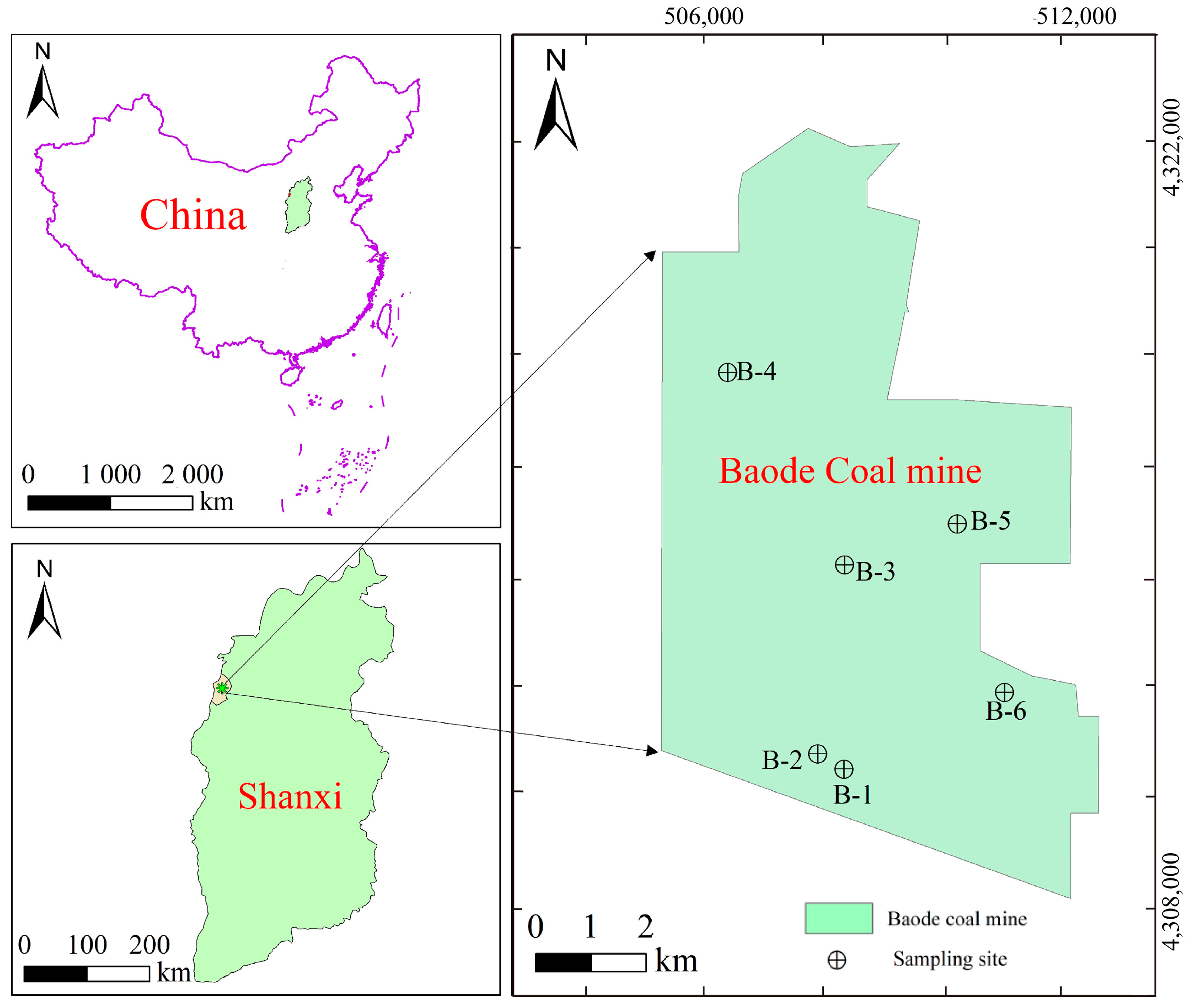
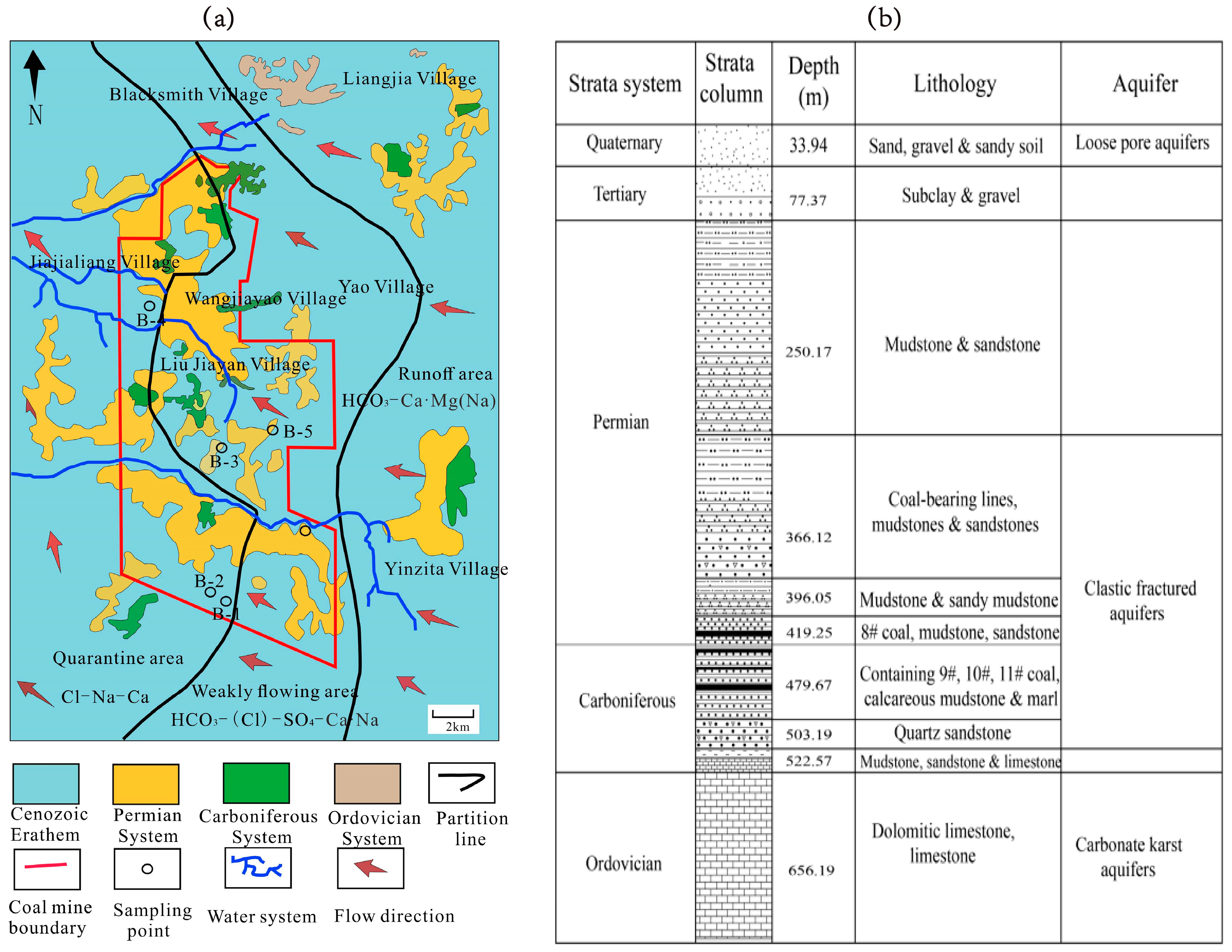
The Baode Coal Mine is situated approximately 13 km east of Baode County in Shanxi Province. The mining area is approximately 5.7 km wide from east to west and 14 km long from north to south, covering an area of approximately 55.9 km² (Figure 1). The overall terrain of the mining area is low in the middle and high in the north and south. The highest elevation is +1148.1 m, and the lowest elevation is +812.2 m at the bottom of Zhujiachuan Ditch. The mine area is largely covered by Cenozoic strata, with only bedrock exposed in the gullies. According to drilling disclosure and surface investigation, the strata in the mining area, from old to new, include Ordovician in the Lower Paleozoic, Carboniferous and Permian in the Upper Paleozoic, and Neogene and Quaternary in the Cenozoic (Figure 2). The Carboniferous and Permian strata are coal-bearing strata; the overlying strata of the coal-bearing strata are loose deposits of the Cenozoic, and the underlying strata of the coal-bearing strata are Ordovician strata, which are the base of the coal-bearing strata. The main coal seams in Baode Coal Mine are 8#, 10#, and 11#, of which the main coal seam (8#) is located in the Permian Shanxi Formation; 10# and 11# are located in the Carboniferous Taiyuan Formation. The Ordovician limestone aquifer under the 8#, 10#, and 11# coal floors is the main aquifer that affects the safe mining of these seams.

The aquifers in the well field mainly include the Cenozoic loose rock-like pore aquifer and the Carboniferous and Permian bedrock fissure aquifer, as well as the Middle Ordovician carbonate rock karst aquifer. The Neoproterozoic and Quaternary are recharged locally and discharged nearby, and the water chemistry type is mainly HCO₃-Ca-Mg type water. The Carboniferous and Permian strata are exposed in small areas and receive limited recharge from various sources, which is slowly transported to depth along weak fissures in the rock layer, and the hydrochemical type is dominated by HCO₃-SO₄-Na-Ca type. The Ordovician limestone water from the eastern boundary of the well field to the western boundary is in the order of runoff zone, weak runoff zone, and stagnant flow zone (Figure 2a). The Ordovician limestone outcrop area outside the eastern well field receives atmospheric precipitation infiltration and surface water infiltration as the main sources of recharge, and generally runs off along the northeastern, eastern, and southeastern directions to the western Yellow River in the direction of the Tianqiao spring group, and the discharge channel is the Tianqiao spring group. Within the well field, the Ordovician limestone water is in a closed state with long-term stagnating flow, poor recharge conditions, slow hydraulic slope, and weak underground runoff. Therefore, its water quality is basically maintained in the original natural state without human interference, and the hydrochemical type is mainly HCO₃-Na·Mg water.

3. Materials and Methods

3.1. Data Acquisitions

Goaf water is known as the first killer of mine water disasters in China [28]. This experiment mainly takes goaf water from several goaf areas in Shanxi Baode Coal Mine and the mixed water of goaf water mixed with Ordovician limestone water as the research object. Under the guidance of water prevention and control professionals in Baode Coal Mine, according to the characteristics of the water sources of mine water inrush in Baode Coal Mine, six groups of water samples were selected scientifically, including goaf water, sandstone fissure water, and Ordovician limestone karst water. Four of these were collected from goaf water from different goaf areas (B-1, B-3, B-4, B-5). One was collected from karst aquifers (B-2), and one was collected from bedrock fissure aquifers of coal-derived sandstone fissure water (B-6). The mine water chemistry data are shown in

Table 1. Water sample information.

Number	Sampling Location	Water Type	pH	Main Ion Concentration (Unit: mg/L Except for pH)
				Ca2+	Mg2+	Na+ + K+	SO42−	Cl−	HCO3−
B-1	308 mining area	goaf water	7.40	75.18	33.21	100.62	8.20	134.70	615.06
B-2	Observation hole2	Karst water	7.61	77.35	33.32	293.58	156.82	546.04	42.10
B-3	203 mining area	goaf water	7.60	40.67	13.67	236.30	5.04	161.83	547.78
B-4	507 mining area	goaf water	8.70	11.12	2.11	426.23	16.50	108.51	797.19
B-5	104 mining area	goaf water	7.30	129.90	63.37	85.07	113.89	93.27	642.64
B-6	13# coal seam	Fissure water	8.00	112.81	58.52	73.54	840.09	102.10	445.71

, and the distribution location of water sample collection points is shown in Figure 1. Since sampling points B-1 and B-2 are spatially adjacent, this study mixed the goaf water from B-1 with Ordovician limestone karst water from B-2 at volume ratios ranging from 1:9 to 9:1, and performed spectral analysis and identification on these mixed water samples. In this study, the UV-1700PC ultraviolet–visible spectrophotometer (Shanghai Meixi Instruments Co., Ltd., Shanghai, China) was used to measure the UV–Vis spectra of the collected water samples at room temperature [29]. The measurement wavelength range was set from 190 to 1100 nm, with a resolution of 1 nm and a cuvette path length of 1 cm. The spectrophotometer was baseline calibrated using ultrapure water as a blank control [30]. Each sample was measured independently 20 times, and the average value was taken as the measurement result. A total of 300 sets of sample data were obtained. To prevent the influence of factors such as temperature, humidity, and background light on the test, the ultraviolet–visible spectrophotometer was preheated for 15 min before scanning the spectra of the mine water samples, and then calibration and parameter settings were carried out. At the same time, the collected water samples were sent to the Hebei Provincial Environmental Monitoring Institute for water chemistry testing, including pH, total hardness (TH), total dissolved solids (TDS), Na⁺, K⁺, Ca²⁺, Mg²⁺, Cl⁻, HCO₃⁻, and SO₄²⁻ ions. The parameters such as temperature, pH, and TDS were tested on-site using a portable multi-parameter water quality tester (Multi 350i/SET, WTW, Weilheim, Germany). The spectrophotometer (Dionex-2500 type, Thermo Fisher Scientific, Waltham, MA, USA) was used to determine the mass concentration of SO₄²⁻ and Cl⁻. The inductively coupled plasma spectrometer (ICAP 6300Duo type, Thermo Fisher Scientific, Waltham, MA, USA) was used to determine the ions of K⁺, Na⁺, Ca²⁺, and Mg²⁺. The mass concentration of HCO₃⁻ was determined by titration. To ensure the authenticity and reliability of the experimental data, all collected water source samples need to be sealed and protected from light.

3.2. Methods

The traditional water chemistry-based approach to mine water sources requires a series of methods such as cautery and titration to test the pH, hardness, and ion concentrations of various components of the water sample, which can be time-consuming. In addition, the water chemistry data is of different orders of magnitude, and a single sample has a large impact on the discriminative process of the model, so the data needs to be normalized and pre-processed before training. In view of the above problems, this study proposes a mine water inrush source identification method based on UV–Vis spectrophotometry and a convolutional neural network algorithm. The absorbance spectral line image of the detection sample is directly taken as the input data, and the feature extraction of the mine water source sample image is carried out by a convolutional layer, which not only avoids the extremely time-consuming detection process, but also reduces the tedious pre-processing process such as standardization, denoising, and feature extraction during spectral data identification [31]. In this method, features of different water samples are selected and distinguished by an iterative process with high network depth and high training degree. On the premise of improving the recognition ability, it also avoids the traditional water chemical sample test and data pre-processing process, and achieves the purpose of rapid and efficient recognition.

To verify the efficiency of this method, the author also conducted a comparative experiment. The UV–Vis spectrophotometry combined with a convolutional neural network (UV–CNN) was compared with the hydrochemical-based kernel principal component analysis-support vector machine (KPCA–SVM). UV–CNN takes the absorbance line image as the input data and classifies the absorbance line graph of the water sample by using convolutional neural network image recognition. KPCA–SVM takes water chemical parameters as input data and adopts support vector machine (SVM) as a classification method to discriminate after data enhancement and KPCA dimension reduction.

3.2.1. Convolutional Neural Network Model

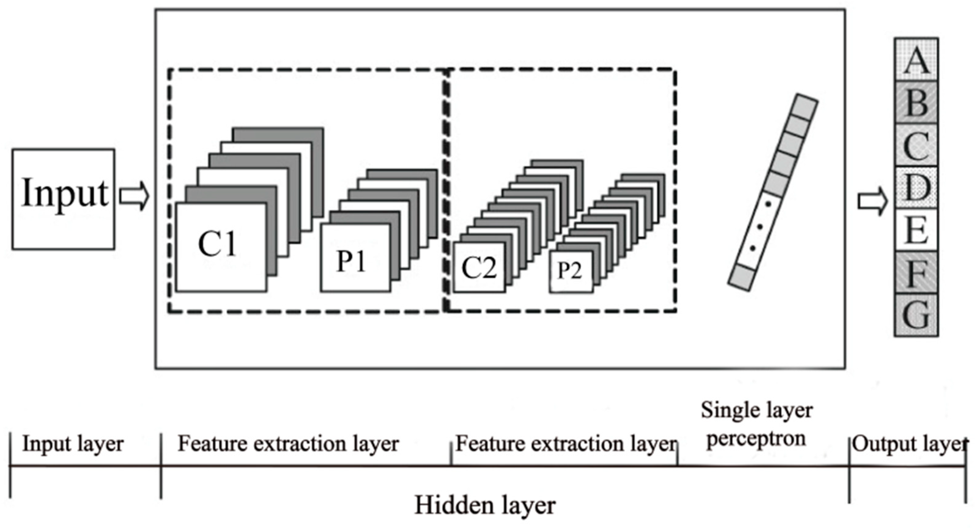
The convolutional neural network (CNN) is the most important supervised learning algorithm in the field of deep learning and has a wide range of applications in image processing [32]. The convolutional neural network is generally composed of an input layer, hidden layer, and output layer (Figure 3). The input layer is the original image without processing, the output layer is the result of feature classification, and the hidden layer is a complex neuron layer with a multilayer non-linear structure, including the repeated structure of convolutional layers and pooling layers and the single-layer perceptron. The feature extraction and classification of the convolutional neural network are carried out in the hidden layer, so the optimization of the convolutional layer and single-layer perceptron can improve the accuracy of feature extraction and optimize the effect of classification. Figure 3 illustrates the convolutional neural network structure model with only two convolutional layers (C1 and C2) and two pooling layers (P1 and P2) in the hidden layer. The input data in the figure is the original image, and the results of the output layer are divided into seven categories: A~G. The repeated structure composed of layer C and layer P is used as the basic unit of feature extraction. After several feature extractions, the final feature map is rasterized to obtain a one-dimensional matrix, namely the fully connected layer. The final output results are obtained by the fully connected layer and the output layer.

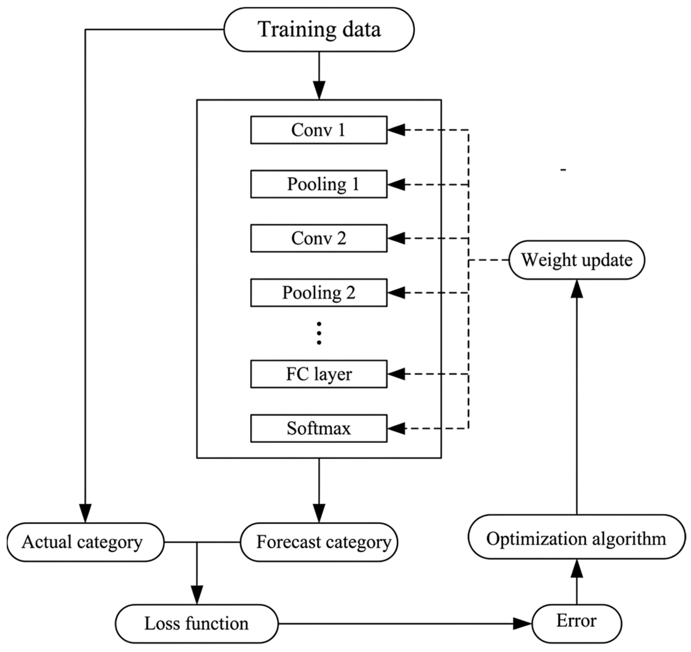
The layers are interconnected to form a network structure. After the input layer is fed with a spectral image, the convolution layer uses multiple convolution kernels to obtain a feature map after convolution operations; the pooling layer is used to extract local features of the data, and after one or more fully connected layers, the features can be mapped to the sample space for classification. The activation function uses a non-linear ReLU function to avoid the gradient disappearance problem [33]. In contrast, in the classification problem, the final layer of the neural network uses a Softmax function that maps the input to values between 0 and 1 as the probability of the corresponding category [34]. The model is trained by first initializing the weights and inputting a spectral map of the absorbance of the water source sample, which is fed into the neural network from the input layer and passed forward through the hidden layer to reach the output layer to obtain the prediction result. The error is then passed backwards, calculating the error between the predicted and actual results of the model, passing the error through the output layer to the hidden layer and backwards to each of the previous neurons, while updating the weights and biases between the layers in turn in conjunction with the optimization algorithm, repeating these processes over and over until the error in the output layer is less than the expected value. Among them, the reverse transfer of the fully connected layer is based on the chain rule of derivatives to calculate the gradient of the previous layer, while the convolutional layer is calculated by flipping the convolutional kernel and the reverse pooling of the error. The flow chart of the error reverse transfer method is shown in Figure 4.

3.2.2. Realization of Dual Optimization of Convolutional Neural Network

In order to construct the convolutional neural network model of convolution optimization and single perceptron optimization, the convolution optimization model and the full-connection optimization model should be designed. The construction principle of the optimized convolution model lies in the iterative optimization of convolution kernel weights. Specifically, the weights and bias terms of the dataset are learned and solved based on small-scale data samples to further generate a sparse feature matrix. Meanwhile, the initial parameters of the convolution kernel are assigned under the constraint of convolution coefficients. The detailed solution procedure for feature matrix S is presented as follows:

Let matrix X denote the sample dataset, matrix A represent the basis matrix that maps X from the sample space to the feature space, and matrix S correspond to the feature representation of the dataset. The optimization of matrix S is implemented by constructing the objective function J(A, S), initializing the value of S, and minimizing the objective function iteratively. Assigning a high-quality initial value to S could prevent poor convergence performance during iterations, thereby achieving faster convergence speed and more optimal solutions. The initialization of S and the subsequent feature updating procedure are described as follows:

$$S=G\left(W^T\mathrm{X}\right),S_c^{\prime }={\displaystyle \frac{S_c}{{\left|\left|A_c\right|\right|}_1}}$$

(1)

where $W^T$ is a random orthogonal matrix; $S_c$ denotes the cth eigenvector matrix of matrix $S$; and $A_c$ denotes the basis matrix corresponding to $S_c$ in matrix A.

Suppose M is an m × n matrix:

$${\left|\right|M\left|\right|}_k={\left({\displaystyle {\sum }_{i=1}^m}{\displaystyle {\sum }_{j=1}^n}{\left|m_{ij}\right|}^k\right)}^{{\displaystyle \frac{1}{k}}}$$

(2)

This normalization process can maintain the sparse structure while ensuring the performance of the algorithm. Through the aforementioned procedure, an ideal initial solution can be generated for S, and the specific expression of its objective function is as follows:

$$J\left(A,S\right)={\left|\right|AS-X\left|\right|}_2^2+{\gamma \left|\right|A\left|\right|}_2^2$$

(3)

In the formula, ${\left|\right|AS-X\left|\right|}_2^2$ represents the residuals of the sample set reconstructed from the basis matrix and the feature set and the measured sample set. ${\gamma \left|\right|A\left|\right|}_2^2$ is a sparse constraint term, and parameter $\gamma$ is the sparsity coefficient.

The steps for iterative solution of S are as follows:

Step 1: Initialize a random matrix A.

Step 2: According to the given A and S, the local optimal solution of the objective function J(A, S) is solved by gradient descent, and the updated S′ is obtained. The parameter α is the step size, which regulates the change amplitude of each round of gradient iteration. The detailed calculation steps are as follows:

$$S^{\prime }=S-\alpha {\displaystyle \frac{\partial J(A,S)}{\partial S}}$$

(4)

Step 3: Based on the updated matrix S′, the gradient descent algorithm is once again enabled to conduct local optimization on the objective function J(A, S), and the iterative update result A′ is obtained.

$$A^{\prime }=A-\alpha {\displaystyle \frac{\partial J(A,S)}{\partial S}}$$

(5)

Step 4: Assign the iteratively updated A′ and S′ to the matrices A and S, and repeat the iterative processes from steps 2 to 4. Affected by the inherent characteristics of the gradient descent algorithm, the objective function will continue to decrease along the opposite direction of the gradient. The iterative operation continues until the gradient vector approaches zero and the objective function converges to almost no fluctuation.

The dual optimization algorithm relies on convolution optimization and fully connected optimization to improve the feature extraction accuracy and classification ability of convolutional neural networks [35]. Suppose the convolutional neural network contains k convolution layers; the size of each convolution kernel is $l_{ker}$ × $l_{ker}$, the input image size of the convolutional layer is the matrix of $l_{img}$ × $l_{img}$, and the number of input and output feature graphs or images is $n_{in}$ and $n_{out}$, respectively. The initialization process for the convolution kernel is as follows.

Let the matrix ${Mat}_1$ be the characteristic matrix S when the objective function obtains the minimum value after many iterations. The convolution coefficient is used to optimize the convolution kernel, and the function expression is constructed according to the interpolation principle. The dynamic convolution coefficient $\mu$ expression is as follows:

$$\mu ={\displaystyle \frac{n_{in}{n}_{out}{l}_{img}^2}{2^k}}+{\theta }_1$$

(6)

where ${\theta }_1$ is the correction error term, and the expressions for the number of parameters required by the input data and output data of the convolution check are as follows:

$$f_{in}=n_{in}{l}_{ker}^2 ,{ f}_{out}=n_{out}{l}_{ker}^2$$

(7)

The optimized convolution kernel initialization expression is as follows:

$${Mat}_2=2\sqrt{{\displaystyle \frac{\mu }{f_{in}+f_{out}}}}\cdot {Mat}_1$$

(8)

${Mat}_2$ is the finally determined optimal convolution kernel parameter matrix. According to the principle of the fully connected optimization model, the fully connected process of the regression classification is optimized to improve the classification and recognition ability of the network. It is assumed that the convolutional neural network contains k convolutional layers, and all the input images are classified into $n_{cag}$ class. The number of iterations required by the convolutional neural network is ε. The number of feature graphs generated by the last sub-sampling layer received by the single-layer perceptron is $n_f$. The optimization process of fully connected parameters is similar to that of convolution optimization, and the process is as follows.

Suppose ${Mat}_3$ is a fully connected parameter matrix randomly initialized with parameters $n_{cag}$ and $n_{f{l}_{img}^2}$. According to the operation process and classification results of a convolutional neural network, the parameter setting of the fully connected layer is affected by the number of convolutional neural network iterations and other factors. According to the interpolation principle, the constructors optimize the fully connected parameters and set $\rho$ as the optimization coefficient:

$$\rho ={\displaystyle \frac{n_{cag}}{2}}(\omega -\epsilon k^{\epsilon -1})$$

(9)

where $\omega$ is the factor affecting the optimization coefficient, which is determined by the amount of data processed by the single-layer perceptron and the number of classifications. Set ${\theta }_2$ as the correction error term.

$$\omega =\left[\lambda \left(\sqrt{n_{f{l}_{img}^2}}-n_{cag}\right)-k^{\epsilon }\right]+{\theta }_2$$

(10)

$$\lambda =k+{\displaystyle {\sum }_{i=0}^{\epsilon -1}}i$$

(11)

Suppose ${Mat}_4$ is the parameter matrix of the final fully connected layer, and the optimized parameter expression of the fully connected layer is

$${Mat}_4=2\sqrt{{\displaystyle \frac{\rho }{n_{cag}+n_{f{l}_{img}^2}}}}\cdot {Mat}_3$$

(12)

The fully connected layer optimization of the double-optimal dual-optimization model needs to accept the convolution parameter as an input parameter of the algorithm. $\rho$ is the coefficient when only the fully connected layer is optimized; ${\mu }_0$ is the original convolution coefficient; and $\mu$ is the optimized convolution coefficient. $\omega$ is the factor affecting the optimization coefficient in the dual optimization algorithm; the expression for the optimization coefficient $\eta$ expression of the algorithm is

$$\eta ={\displaystyle \frac{{\mu }_0}{{\mu }_0+\mu }}\rho +{\displaystyle \frac{\mu }{{\mu }_0+\mu }}(\omega -k^{\epsilon })$$

(13)

The process of solving the fully connected parameter matrix of the updated single-layer perceptron ${Mat}_4$ is as follows:

$${Mat}_4=2\sqrt{{\displaystyle \frac{\eta }{n_{cag}+n_{f{l}_{img}^2}}}}\cdot {Mat}_3$$

(14)

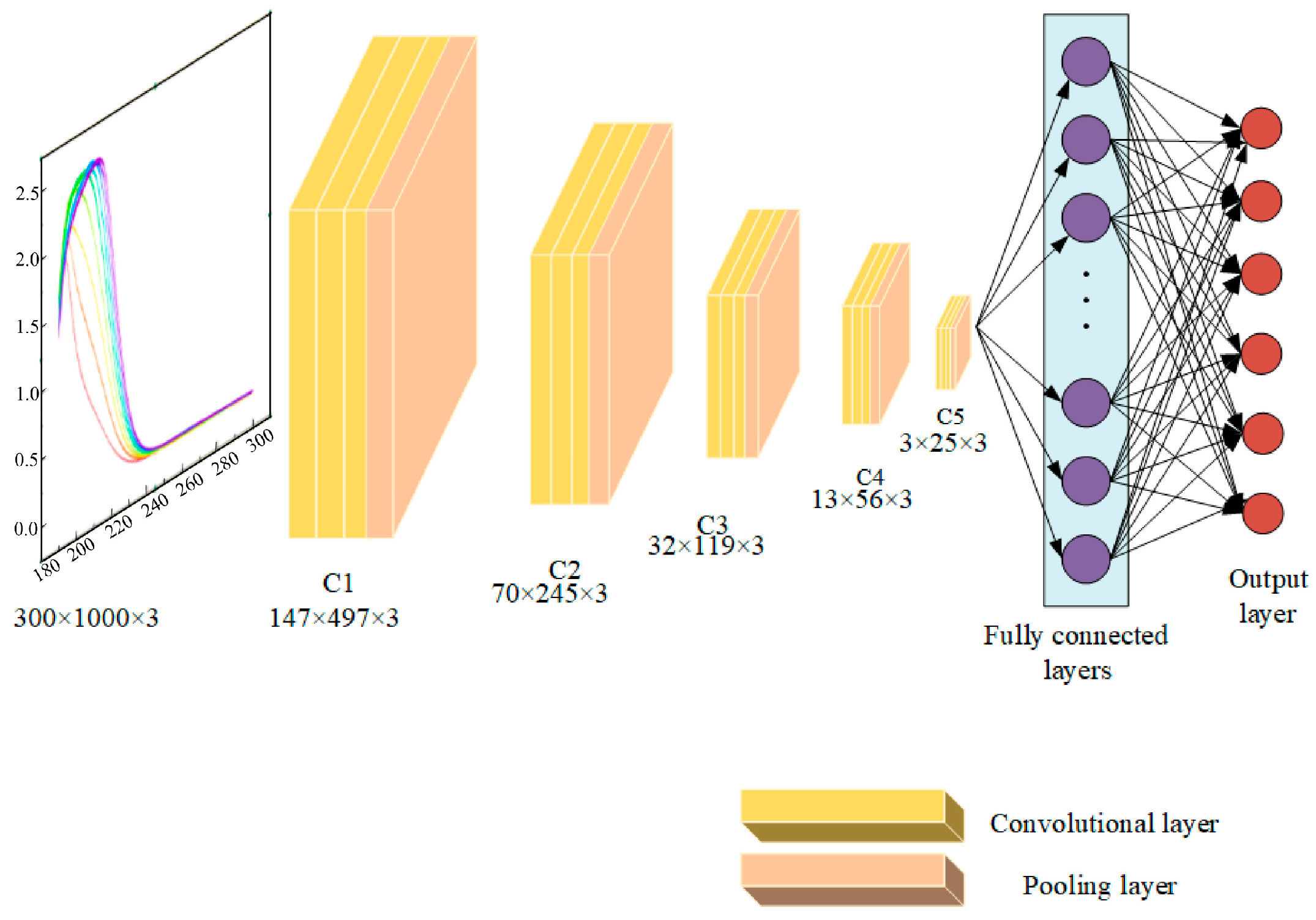
This study constructed an 8-layer convolutional neural network (CNN) model, comprising an input layer, convolutional-pooling layer group C1, convolutional-pooling layer group C2, convolutional-pooling layer group C3, convolutional-pooling layer group C4, convolutional-pooling layer group C5, a fully connected layer, and an output layer. The conceptual framework of the model is shown in Figure 5. All convolutional layers consist of three convolution kernels, each with a size of 8 × 8 and a step size of 1, and the activation function is the ReLU function. The size of the pooling layer is 8 × 8, the step size is 2, and the maximum pooling method is adopted. The fully connected layer has 1125 neurons, and the activation function is the ReLU function. The number of neurons in the output layer is the number of categories of data. Feature extraction and classification learning are carried out synchronously in the training process, and the parameters of network training are reduced by weight sharing and local connections. The feature acquisition process of images does not need to be extracted manually in advance, and the features acquired by the learning process have strong mapping ability and generalization ability. Meanwhile, the classification accuracy improves with the deepening of the network depth.

3.2.3. Support Vector Machine Model

Support vector machines (SVMs) are generally used to solve two-class classification problems, and now they can also handle multi-classification problems. The basic principle is to find a hyperplane ${\omega }^T{x}_i+b$, so that the points of different categories in the training set fall on both sides of the hyperplane [36]. The machine learning method can use different kernel functions to map samples to a high-dimensional space to find a hyperplane. Therefore, the support vector machine can perform linear classification and non-linear classification.

For a linearly separable dataset, the objective function is

$$min={\displaystyle \frac{1}{2}}{‖\omega ‖}^2$$

(15)

Obey the constraints:

$$y_i\left({\omega }^T{x}_i+b\right)\ge 1, i=\mathrm{1,2},\cdots ,n$$

(16)

For the linearly inseparable dataset, the relaxation coefficient ξi ≥ 0 and the penalty factor C are introduced, and the objective function and constraint conditions become (12) and (13)

$$min={\displaystyle \frac{1}{2}}{‖\omega ‖}^2+C {\sum }_{i=1}^N{\xi }_i$$

(17)

$$y_i\left({\omega }^T{x}_i+b\right)\ge 1-{\xi }_i , i=1, 2,\cdots ,$$

(18)

In the formulas, $n$ is the number of samples, ω and b are the weight and bias parameters of the hyperplane, respectively, and x_i and y_i represent the i-th input vector and the i-th dependent variable values, respectively. The above extremum can be solved using the Lagrange multiplier method [37].

3.2.4. Kernel Principal Component Analysis (KPCA)

Kernel principal component analysis (KPCA) is a commonly used non-linear dimensionality reduction algorithm. It can transform data from a high-dimensional space to a lower-dimensional space while retaining the main features of the data [38]. KPCA calculates the inner product of sample similarities through the kernel function [39], ultimately achieving non-linear dimensionality reduction, feature separation, fault identification, and other statistical analyses. The general algorithm steps of KPCA are as follows:

There are m sets of n-dimensional data. The original input data are combined into a matrix X with n rows and m columns.

$$\left[\begin{array}{ccc}{x}_{11}& \cdots & x_{1m}\\ ⋮& \ddots & ⋮\\ x_{n1}& \cdots & x_{nm}\end{array}\right]$$

(19)

Select the kernel function, calculate its matrix K, and perform centering processing to obtain H.

$$H=K-l_{N}K-K{l}_N+l_N^{T}K{l}_N$$

(20)

Among them, $l_N$ is an N × N matrix filled with all 1 s, which is used to eliminate the influence of the data mean on the subsequent analysis.

Calculate the eigenvalues λ and eigenvectors α of the centralized kernel function matrix H as follows.

$$H\alpha =\lambda \alpha$$

(21)

The feature vectors are normalized to obtain the feature vectors.

$${\mu }_1,{\mu }_2,\cdots ,{\mu }_n$$

(22)

Set the cumulative contribution value ε, and select the top t feature values based on the degree of contribution.

$${\lambda }_1,{\lambda }_2,\cdots ,{\lambda }_t$$

(23)

Calculate the projection W of the matrix H onto the eigenvectors.

$$\mathrm{W}=\mathrm{H}·\left[{\mu }_1,{\mu }_2,\cdots ,{\mu }_t\right]$$

(24)

4. Results and Discussion

4.1. Spectral Data Screening and Analysis

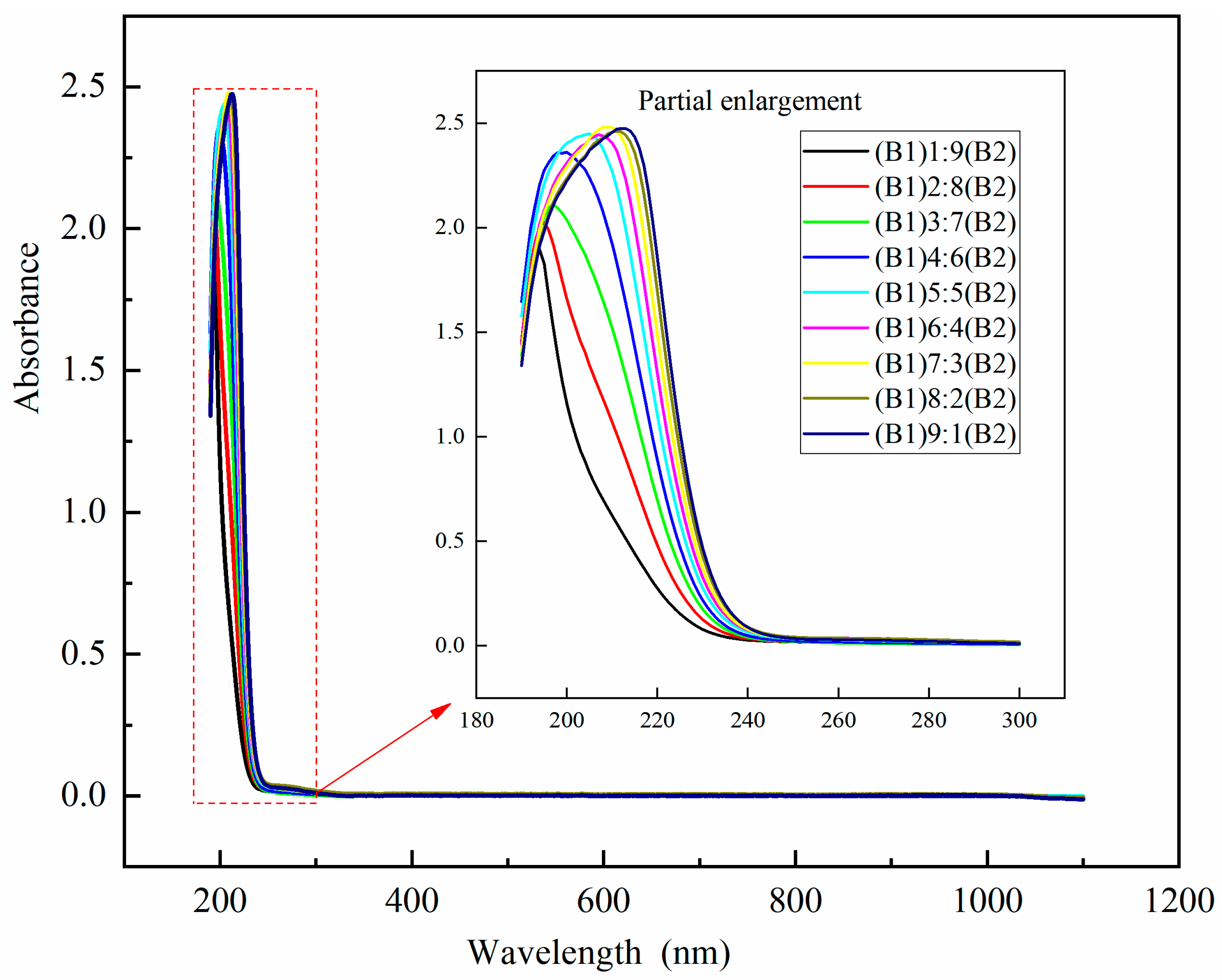
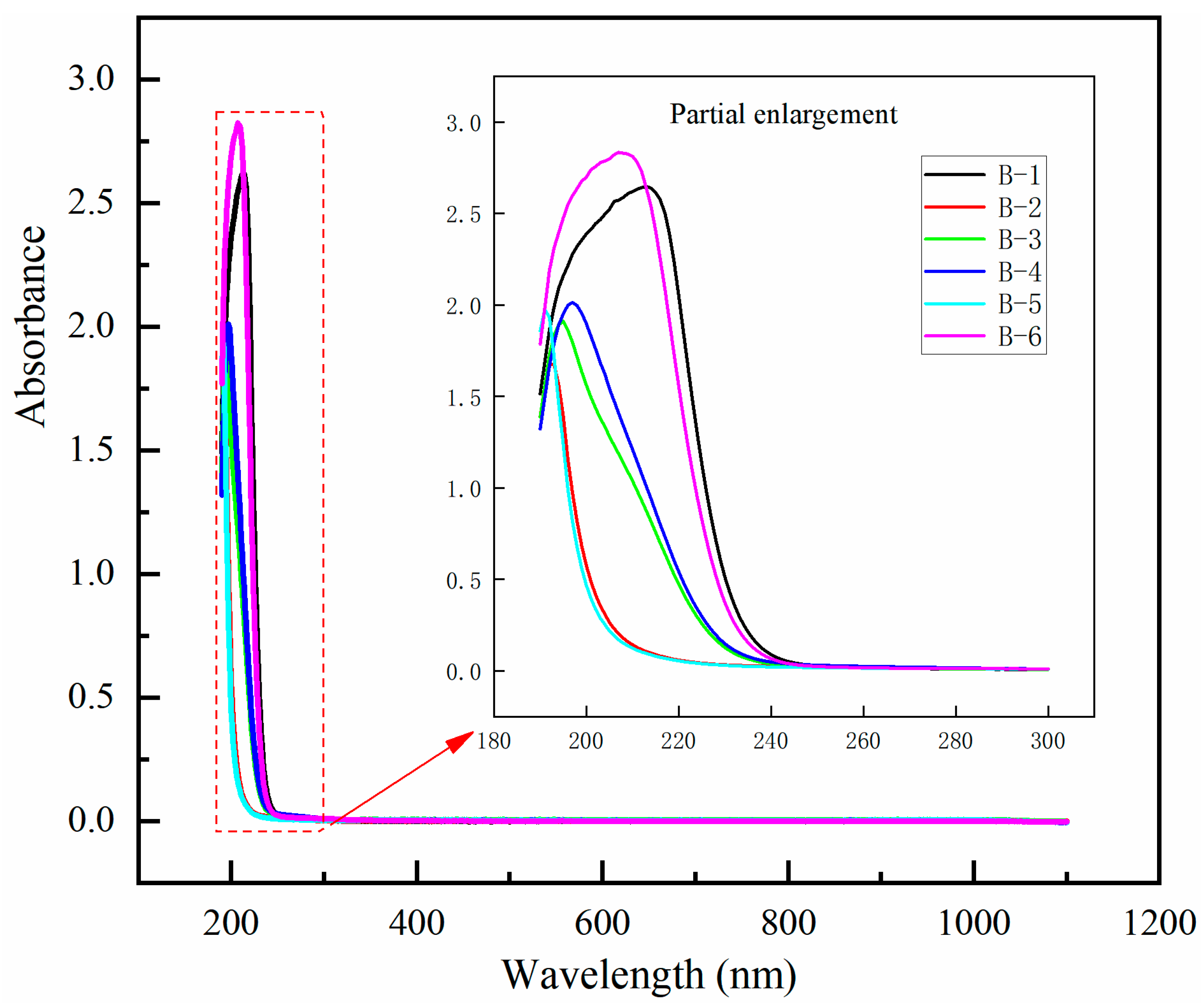
The spectral data of single and mixed water samples were determined using a spectrophotometer. The experiment used full-band data, and the wavelength range is between 190 and 1100 nm. Through analyzing spectral image observations, it was found that in the lower-energy (300–1100 nm) long-wavelength region, the experimental samples do not have the absorption ability of functional groups, so the sampling between 190 and 300 nm band absorbance spectral lines was prioritized. The absorbance spectra were collected for six groups of single water samples and B-1 and B-2 mixed water samples prepared at ratios ranging from 1:9 to 9:1, and the absorption spectra of samples at 190–300 nm are shown in Figure 6 and Figure 7. The absorption wavelength of each water sample in Figure 6 is mainly distributed between 190 and 250 nm. The absorbance of goaf water B-3, B4, and B5 is about 2.0, and the maximum absorption wavelength of the three water samples is less than 200 nm. The maximum absorbance of the B6 coal-measure sandstone fissure water sample is 2.82, and after reaching the maximum peak, the absorbance decreases rapidly with the increase in wavelength. Figure 7 shows the absorption spectra of mixed water samples at 1:9–9:1 ratio of B-1 and B-2 in Baode Coal Mine. The wavelength distribution of each proportion of absorbance is mainly affected by the single B-1 and B-2 water samples, and the wavelength range is between 190 and 250 nm, which is arranged in a regular order according to the mixing proportion. As the proportion of the B1 water sample increases, the absorbance value increases, and the maximum absorption peak of the absorbance spectrum line shifts from B-2 to B-1 with the increase in wavelength.

4.2. Hydrochemical Data Processing

Based on the hydrogeochemical test results of the mine water (Table 1), appropriate characteristic ions were selected as analytical indicators. The B-1 and B-2 groups were simulated and mixed by Phreeqc 3.4.0 to obtain the same experimental samples as UV–Vis spectrophotometry. In this research, the author uses min–max standardized line pre-processing, followed by data enhancement and kernel-based principal component analysis (KPCA). The data enhancement technology introduces some types of transformations to expand the number of samples without changing the data labels and key features. Referring to the method of Reference [40], this study expands the number of samples by randomly adding Gaussian white noise obeying a normal distribution to the sample data to be consistent with the data of UV–Vis spectrophotometry. The pretreated hydrochemical data are classified by a support vector machine (SVM) model.

4.3. Model Identification Process

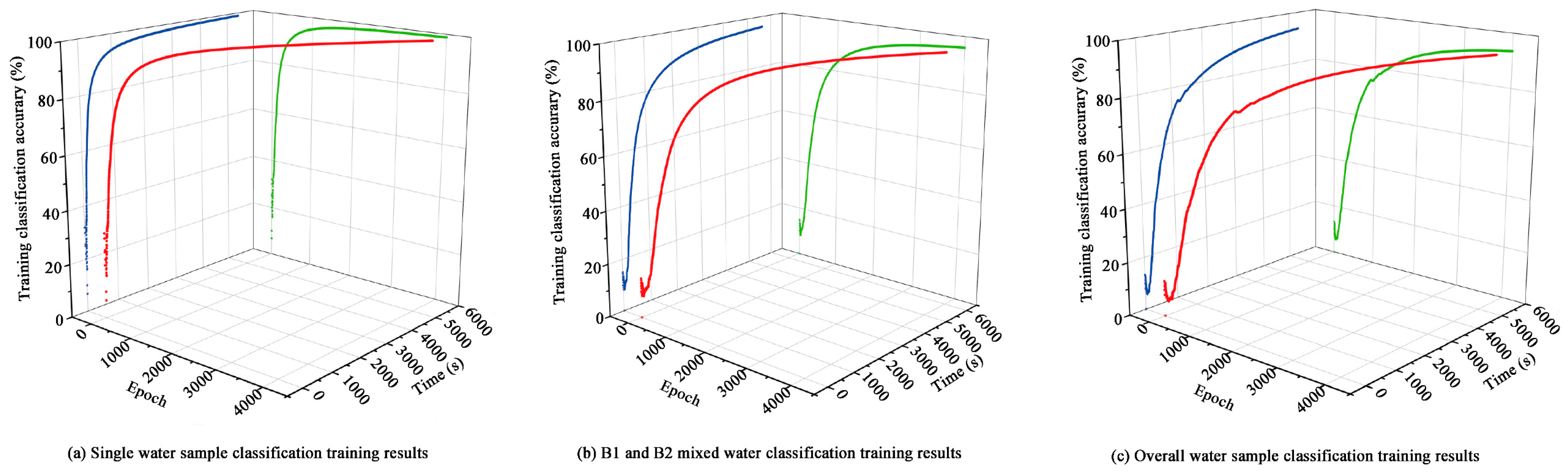
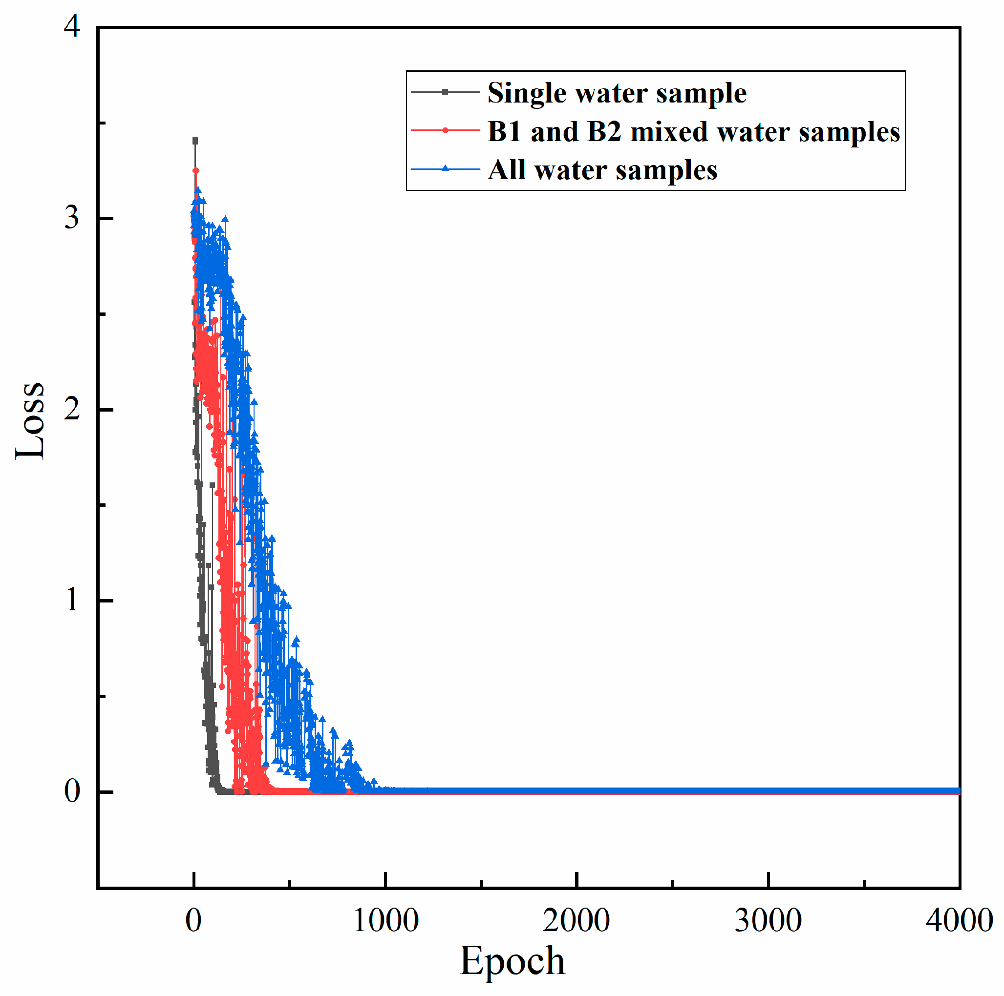
The CNN image recognition was performed with 120 sets of B-1 to B-6 sample spectra and 180 sets of B-1 and B-2 mixed detection spectra with different ratios obtained from the experimental test. To check the image recognition effect, the CNN image recognition was finally performed on the single samples and the mixed samples all together again. In this study, the hierarchical operation of water source spectral images from shallow to deep was carried out through five groups of convolution-pooling layers (C1 to C5), automatically completing the layer-by-layer extraction of spectral features. The shallow convolutional layers (C1~C2) primarily capture the primary visual features of the spectral images. They correspond to the overall contour of the spectral lines, the approximate distribution range of the absorption peaks, and the overall amplitude range of the absorbance shown in Figure 6 and Figure 7. The model can automatically identify 190~300 nm as the effective absorption band, filter out the background noise area of 300~1100 nm without absorption, and automatically locate the core feature area. The middle-level convolution (C3~C4) precisely extracts the spectral line shape differences and further decomposes the spectral line details within the core band into features. For the category differences shown in Figure 6, it accurately captures the peak shape differences in different water samples. For the gradient changes in the mixed water samples shown in Figure 7, it magnifies the minor shifts in peak positions and gradual changes in absorbance amplitudes between adjacent proportion samples. It also converts the nano-level wavelength shifts and 0.1-unit absorbance differences that are difficult to distinguish with the naked eye into quantifiable matrix differences on the feature map. Deep convolution (C5) generates high-order abstract category features. The proportion of the training set, validation set, and test set is 8:1:1. The identification results and loss value changes in the training set for single samples, mixed samples, and overall samples are shown in Figure 8 and Figure 9. The dual optimization mechanism constrains and optimizes the initial values of the convolution kernel by solving for the sparse feature matrix and dynamic convolution coefficients. This avoids the feature shift caused by random initialization, enabling the model to precisely focus on the effective absorption region of 190–300 nm in the early training stage. It significantly accelerates the convergence speed, and the loss value can approach 0 after less than 1000 training iterations (Figure 9). To observe the model training process, no fixed conditions were set for stopping the training. All three models were trained 4000 times. To make the image features more distinct, the RGB values of pixels were retained. The input images were not converted to grayscale, and the data dimensions were maintained during the model training process, which was conducive to the output and observation.

Different mixing ratios of water samples were simulated by Phreeqc 3.4.0, and the data were normalized to [0, 1] by min–max standardization. This was done to prevent any single parameter of the samples from being too large or too small in magnitude, which could cause it to have an excessively high weight in the discriminant model and thereby affect the accuracy of identification. Gaussian white noise that obeys the normal distribution was used to enhance the data. A total of six groups (B-1~B-6) and nine groups of mixed simulation data of B-1 and B-2 were used. Each group is enhanced to 20 samples, for a total of 300 sets of data corresponding to the spectrophotometric experiment. KMO test and Bartlett's sphericity test are performed on the sample data to test whether the correlation is suitable for principal component analysis. The test results show that the KMO value is 0.679 > 0.5, and the Bartlett sphericity test significance value (Sig) is 0.000 < 0.05, so the sample correlation is suitable for principal component analysis. The results of principal component analysis showed that the cumulative contribution rate of the first three principal components was 85.887%, so KPCA was used to extract the three principal components. The cumulative contribution of each principal component and the total variance of the sample data are explained in

Table 2. Interpretation of total variance of sample data.

Ingredient	Initial Eigenvalue
	Total	Percentage Variance	Contribution Rate (%)
1	4.593	45.932	45.932
2	2.286	22.855	68.787
3	1.710	17.100	85.887
4	0.666	6.665	92.552
5	0.446	4.459	97.011
6	0.120	1.201	98.211
7	0.055	0.553	98.764
8	0.047	0.475	99.239
9	0.044	0.438	99.677
10	0.032	0.323	100.000

. F1, F2, and F3 can be used to replace the original 10 evaluation indicators, and the relationship equation is

$$F_1={-0.677H}_1+0.943H_2+0.935H_3+0.898H_4-0.668H_5-0.254H_6+0.457H_7+0.131H_8-0.378H_9-0.828H_{10}$$

(25)

$$F_2=0.103H_1+0.094H_2+0.114H_3+0.158H_4-0.579H_5+0.494H_6+0.132H_7-0.923H_8+0.866H_9+0.171H_{10}$$

(26)

$$F_3=0.696H_1+0.132H_2+0.088H_3+0.191H_4-0.157H_5-0.595H_6+0.789H_7-0.138H_8-0.041H_9+0.038H_{10}$$

(27)

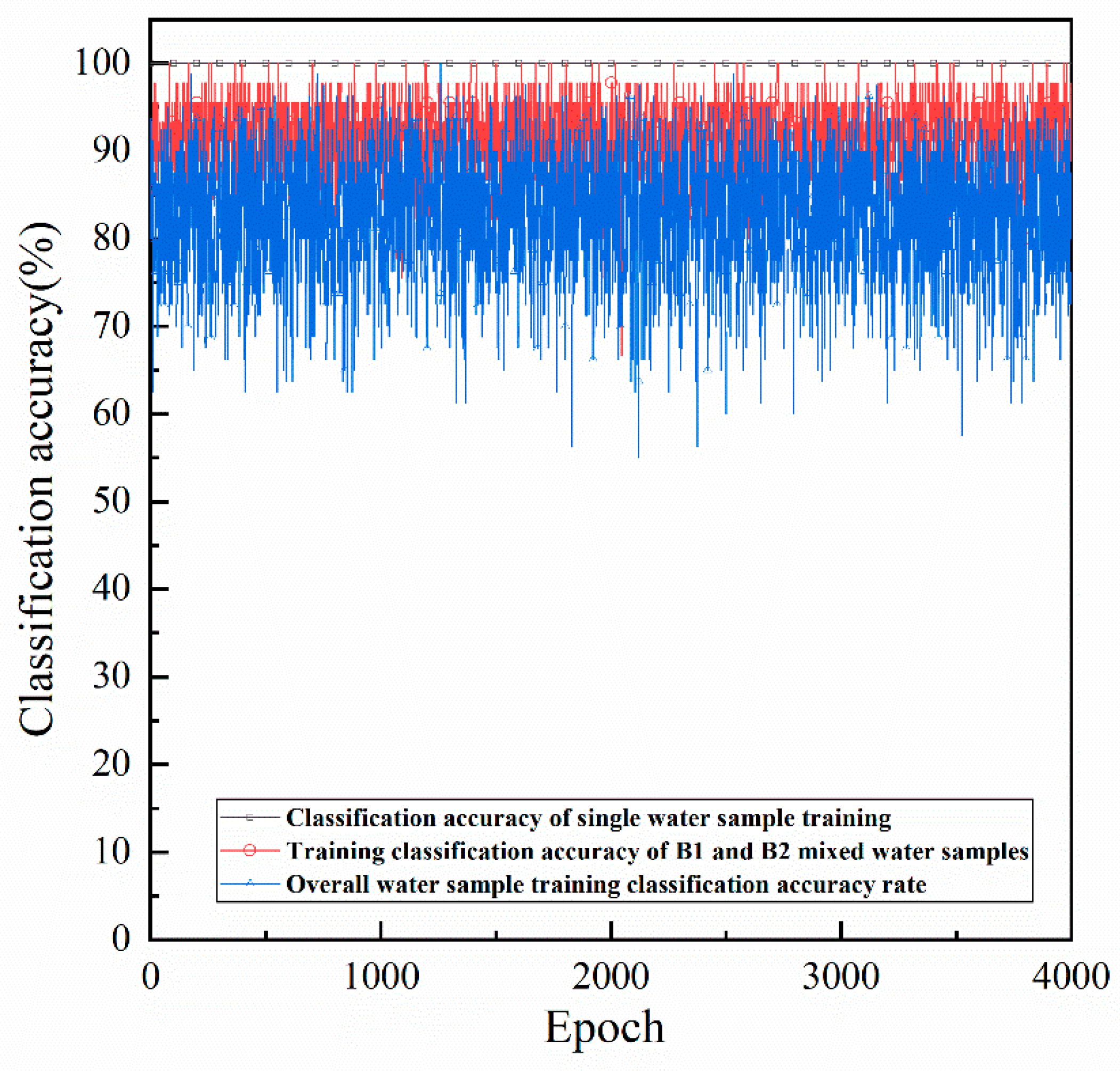
The KPCA extraction result with the kernel function as the radial basis function (RBF) is used as the input data [41]. Similarly, the ratio of training set, validation set, and test set is 8:1:1 for SVM model classification. Since the SVM model is a feedforward network type, the model can be completed in a single training, and no deep iterations can be carried out. However, the accuracy of a single test cannot characterize the performance of the model, so the data is repeatedly trained and tested 4000 times, and the average value is taken as the overall accuracy value. The training process is shown in Figure 10.

The accuracy of the UV–CNN model based on spectral images and the KPCA–SVM model based on water chemistry data in the training set and water sample identification was compared by controlling the same training times of different algorithms. Figure 8a shows spectral samples of six types of single water sources. In the early stage of training, the accuracy rate shows a rapid growth trend, and it only takes 397 s to reach an 85% classification accuracy rate. The final training set has a stable accuracy rate of 98.89%, which is the highest among the three datasets. The accuracy rate throughout the process shows no significant decline or oscillation, and the upward trend is smooth and stable, indicating that the model can quickly complete feature learning for significantly different water source categories and has an excellent fitting effect. Figure 8b shows nine groups of water samples with different mixing ratios. The spectral differences between adjacent ratio samples are extremely small, which is a core verification of the model’s ability to capture subtle features. The convergence speed is slower than that of the single water sample, and it takes 1531 s to reach 85% accuracy. The accuracy rate of the final training set was 95.93%, still maintaining high precision, which verified the learning stability of the model in similar sample scenarios. Figure 8c shows six types of single water samples and nine types of mixed water samples, totaling 15 classification labels. This group has a large number of categories and a wide range of feature similarities, making it the verification group that is closest to the actual water inrush scenario. This group has the slowest convergence speed, needing 3404 s to reach 85% accuracy, and the final training set accuracy is 90.67%. It still maintains an accuracy of over 90% in 15 types of fine classification tasks, fully demonstrating the model’s multi-class robustness. From the training process of CNN image recognition (Figure 8), it can be found that the overall accuracy rate is high in the training process of the model. With a confidence interval of 95%, the accuracy rates of the training set for single water samples, mixed water samples, and overall water samples were 98.89%, 95.93%, and 90.67%, respectively. The accuracy of the whole training process steadily improved, and there was no degradation in turbulence caused by the increase in categories. The convergence process of the model was also relatively fast. Figure 9 shows that within less than one thousand training iterations, the loss values of the three models were all close to zero. This proves that the hierarchical feature extraction architecture of 5 groups of convolution-pooling layers can adapt to the multi-category and differentiated spectral recognition requirements.

The training process of the SVM hydrochemical model based on KPCA dimensionality reduction shows (Figure 10) that the KPCA–SVM is a shallow feedforward machine learning algorithm, characterized by few model parameters and a relatively fast training process. However, this algorithm does not have a deep optimization mechanism of error backpropagation to continuously update weights, and lacks the ability for continuous optimization of representation during training with iterations. Combined with the 4000 training accuracy change curves presented in Figure 10. The training curves of the single water sample group with higher water sample feature discrimination show almost no significant fluctuations. The entire process can stably maintain high-precision discrimination. However, the accuracy curves of the mixed sample groups with high similarity and the overall sample groups with complex categories continuously fluctuate violently within the range of 55% to 95%. There is no stable convergence interval, and the fluctuation amplitude of the model’s discrimination performance is large, and the stability is poor. The mean values of 4000 training accuracies of the SVM model for the training set for single, mixed, and overall water samples were 100%, 91.35%, and 82.87%, respectively. The fluctuating curves shown in Figure 10 demonstrate that the discriminative performance of the KPCA–SVM model is strongly dependent on the sample distribution of randomly partitioned test subsets during model training. When the test set contains numerous mixed water samples with similar mixing ratios and negligible differences in hydrochemical ionic compositions, misclassification events frequently occur, leading to a dramatic drop in overall classification accuracy. In contrast, the model maintains high discriminative accuracy if the test set is dominated by single-aquifer water samples with prominent inter-sample feature disparities. The oscillating fluctuations of the accuracy curves are entirely governed by the sample distribution bias induced by random dataset splitting, which introduces substantial stochasticity into the evaluation results. This indicates that relying solely on the accuracy rate value output by a single training session cannot objectively reflect the real discrimination performance of the KPCA–SVM model in complex mine water gushing source scenarios. More training is necessary to roughly assess its average recognition level.

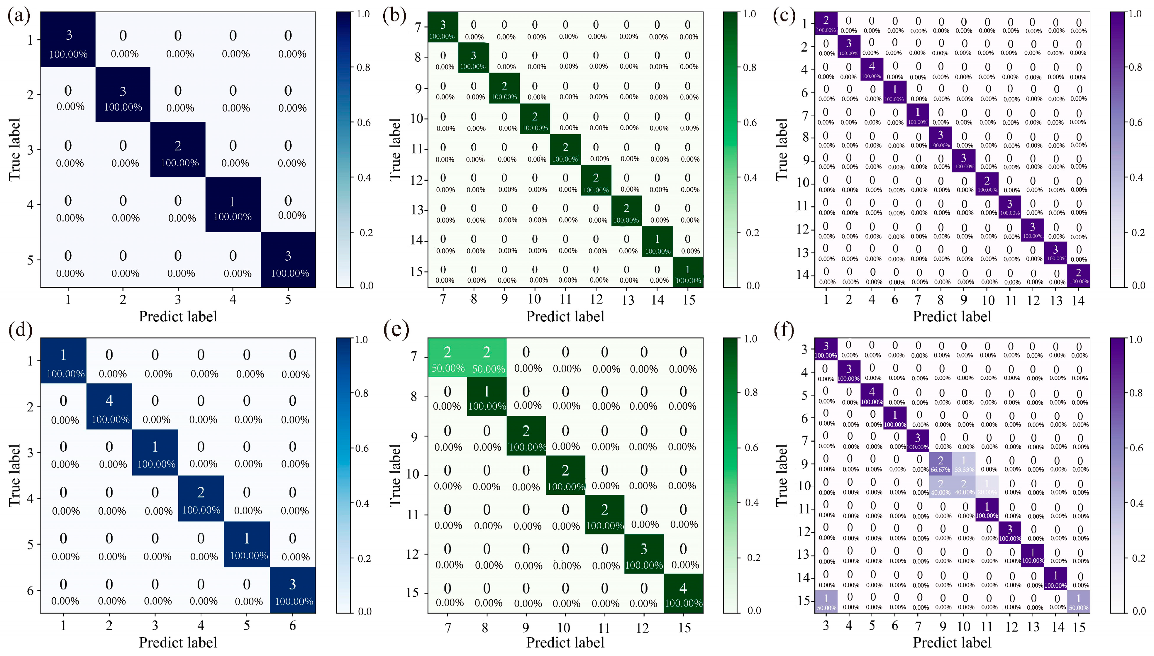
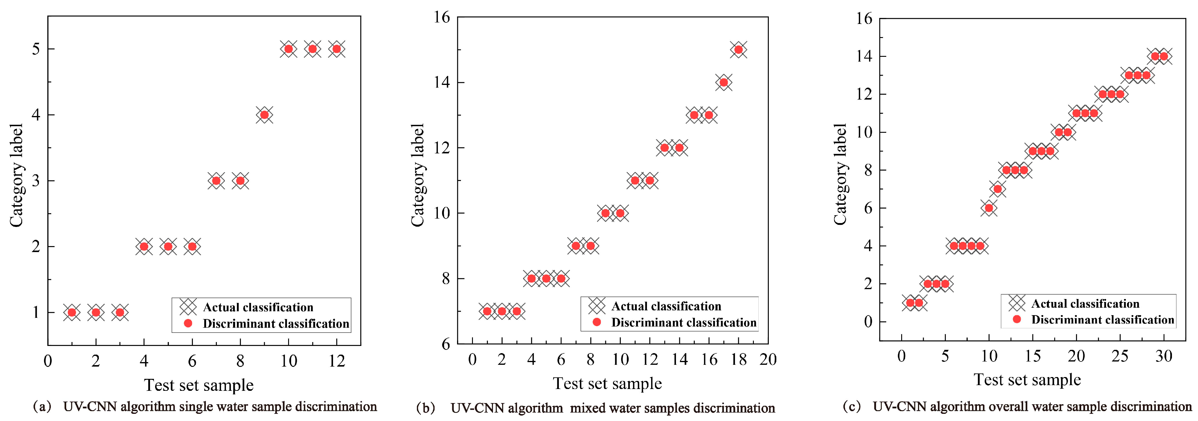
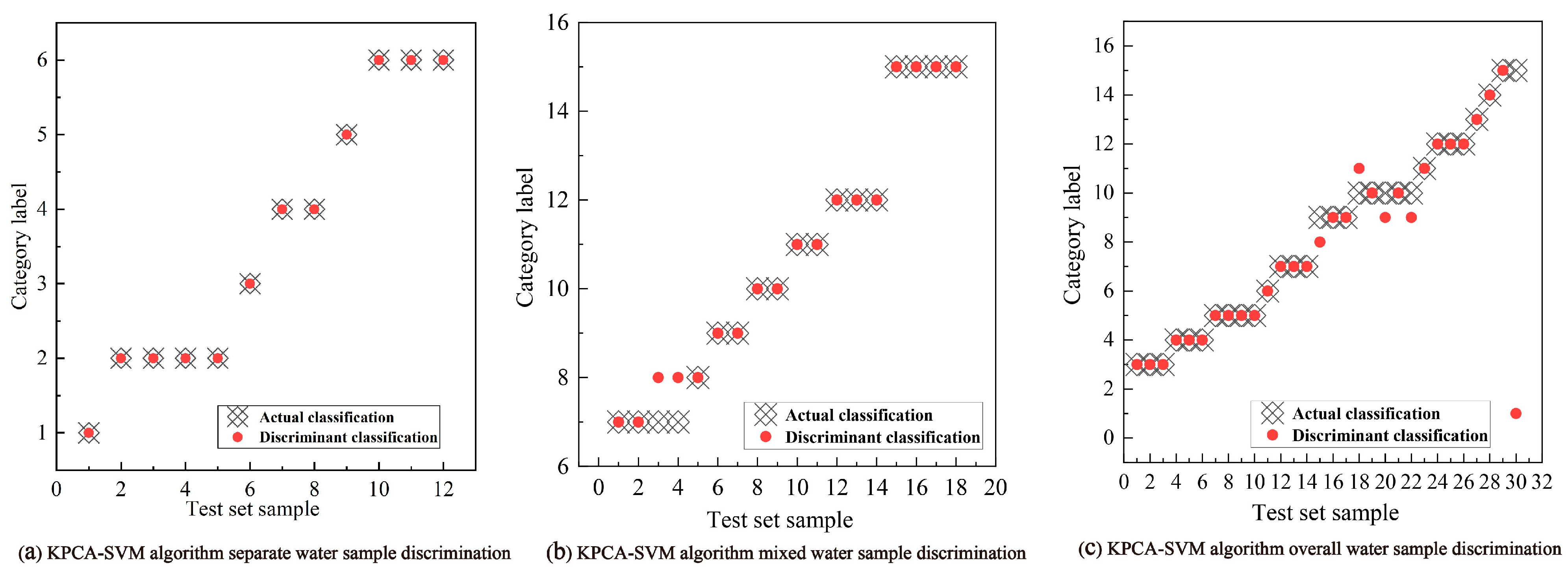
The discriminant results of the two methods on the test set were compared to evaluate their discriminant performance (Figure 11 and Figure 12). The integer between 1 and 20 was used as the classification label for the output, and the sample output labels corresponded to the specific water sample type as shown in

Table 3. Correspondence between output label and sample.

Output Sample Classification Label	The Label Represents The Actual Water Sample Type
1	B-1
2	B-2
3	B-3
4	B-4
5	B-5
6	B-6
7	Mixing ratio of B-1 and B-2 (1:9)
8	Mixing ratio of B-1 and B-2 (2:8)
9	Mixing ratio of B-1 and B-2 (3:7)
10	Mixing ratio of B-1 and B-2 (4:6)
11	Mixing ratio of B-1 and B-2 (5:5)
12	Mixing ratio of B-1 and B-2 (6:4)
13	Mixing ratio of B-1 and B-2 (7:3)
14	Mixing ratio of B-1 and B-2 (8:2)
15	Mixing ratio of B-1 and B-2 (9:1)

, where labels 7–10 had no corresponding water samples. A multi-category confusion matrix is an important tool widely used to evaluate the performance of multi-category models [36]. The multi-category confusion matrix of the UV–CNN model for single, mixed, and overall water samples was presented in Figure 13a–c, respectively, which showed that all the different water categories were recognized correctly. The multi-category confusion matrix of the KPCA–SVM model for single, mixed, and overall water samples was shown in Figure 13d–f. Four mixed water samples with a 1:9 ratio of B1 and B2 were recognized with 50% accuracy, and two samples with a 2:8 ratio were identified incorrectly. In the identification process of 30 samples of all different types, there were as many as five discrimination errors, and the error types were mixed water samples. It can be seen that the classification performance of the UV–CNN model based on spectral data is better than that of the KPCA–SVM model. Especially for mixed samples with small sample differences, the UV–CNN discriminant model shows higher recognition accuracy.

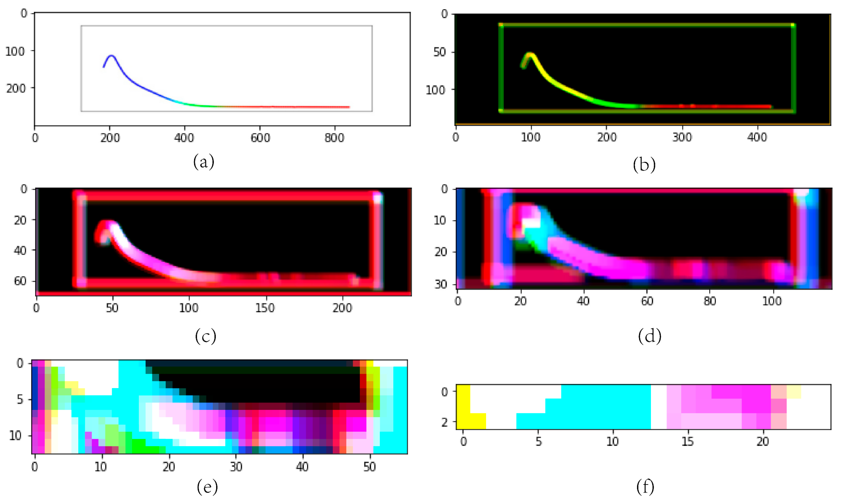
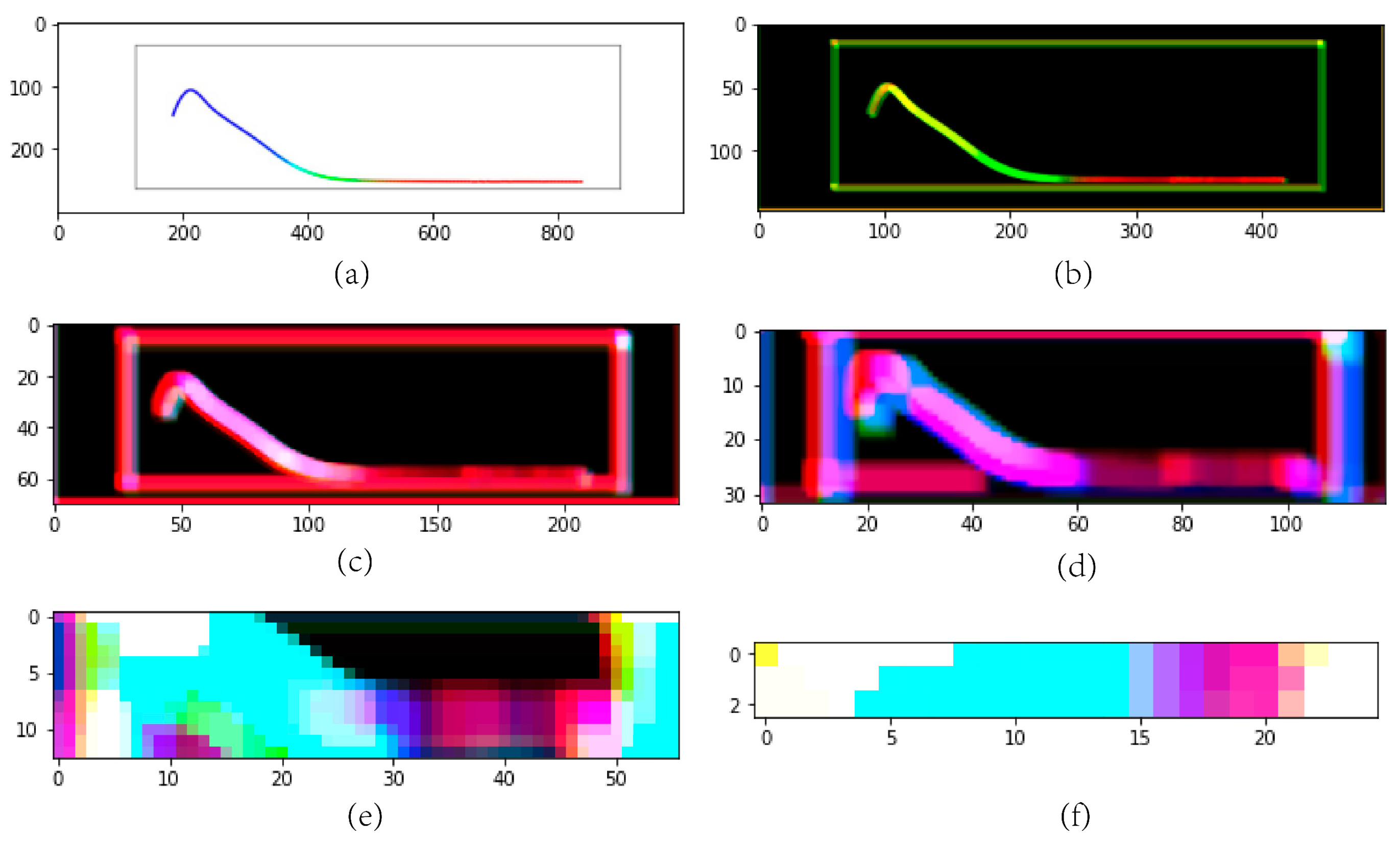
Finally, comparing the classification results of the training set and test set of the UV–CNN and KPCA–SVM models, it was found that the single samples were recognized better and faster by both methods due to the greater inter-sample differentiation. However, when the difference between samples becomes smaller, the double-optimized convolutional neural network has obvious advantages as an intelligent algorithm for iterative optimization calculation. KPCA–SVM model based on water chemistry analysis lacks stability in recognition ability when faced with a large number of samples and a small degree of differentiation between samples. With the deepening of the network layer, the automatic recognition and extraction of image features are more and more obvious. From the feature extraction process of B-1 and B-2 mixed ratio 1:9 samples and 2:8 samples with poor KPCA–SVM recognition and classification effect (Figure 14 and Figure 15), it can be seen that CNN can automatically identify the absorbance spectral line images with major difference features between the wavelengths of 190 nm and 300 nm between the samples, and enlarge them with the increase in network depth. The dual-optimized CNN reduces the dimension of image data by constantly extracting image features, and finally inputs them into the fully connected layer for identification. Since every pixel of an image is composed of three types of RGB data, the difference ratio between samples in the fully connected layer of the CNN has expanded several orders of magnitude compared with that in the input, making it easier to discriminate. Thus, the ability of the dual-optimized CNN to extract differential features from the spectral lines of mine water source samples by using convolution kernels has great advantages over the general feedforward algorithm.

5. Limitations of the Study

This model is a data-driven model, and its discrimination performance is dependent on the completeness of the spectral database. If the database lacks actual water samples of the aquifers existing in the mining area, when faced with unknown water sources as input, the model may make incorrect classifications, which is an important application risk of this method. The experimental samples of this study only covered six types of typical aquifers and nine groups of mixed water samples in the Baode Coal Mine in Shanxi Province, totaling 300 sets of laboratory repeated measurement samples. The sample size is limited by the coverage of the mining area scenario. The generalization performance of the model in other hydrogeological conditions of mining areas and extreme mixed water samples still needs to be verified with larger-scale and multi-scenario datasets. Future research will establish a complete mine water spectroscopy database by collecting mine water samples from different regions and different hydrogeological conditions, further improving the robustness and universality of the model.

Furthermore, the model also encounters practical constraints during its actual application in engineering. The differences in hydrogeochemical conditions of different mines will directly affect the cross-mining transferability of the model. The instrument drift inherent in the UV–Visible spectrophotometer itself can introduce spectral artifacts. However, in multi-device measurement scenarios, the spectral distortion caused by instrument drift will directly alter the input image features, thereby reducing the accuracy of the CNN model’s discrimination. Therefore, research needs to be conducted from multiple perspectives to develop a universal cross-mining district discrimination model, promoting the UV–CNN model from a single-mining district experimental model to a practical engineering discrimination model for multiple mining districts.

6. Conclusions

This study aims to address the technical bottlenecks of the traditional methods for identifying water inrush sources in mines, such as the cumbersome pre-treatment process and the low recognition accuracy of mixed water samples. Taking goaf water, Ordovician limestone karst water, coal measure sandstone fissure water, and their mixed samples from Baode Coal Mine of Shanxi Province as the research objects, a UV–CNN water inrush source discrimination model combining ultraviolet–visible spectrophotometry with a convolutional neural network is established in this study. The model directly takes the absorbance spectral images of water samples as input to the input layer and achieves accurate classification and identification of mine water inrush sources through deep hierarchical feature extraction by the convolutional neural network. The main conclusions are drawn as follows:

The water source discrimination method based on ultraviolet–visible spectrophotometry and a convolutional neural network provides a new idea for the rapid identification of water sources in mine water inrush. The convolutional neural network image recognition technology can converge quickly regardless of whether the sample differences are significant, and can stably improve the training effect. It has good applicability for the training and recognition of the absorbance spectral line image data of water source samples.

The statistical results of model training indicate that UV–CNN has excellent discriminative performance and convergence characteristics for samples of different complexities. The accuracy of the training set for single water source samples, mixed water samples, and all water samples is 98.89%, 95.93%, and 90.67%, respectively. When the accuracy rates of the three training sets reached 85%, the corresponding training times were 397 s, 1531 s, and 3404 s, respectively. The loss value approached 0 after less than 1000 training iterations. The accuracy rate over the entire 4000 training iterations steadily increased without significant oscillations, and the model’s fitting effect and stability were excellent.

The test results show that the UV–CNN model has a 100% accuracy rate in classifying single water samples, mixed water samples, and all water samples. There were no misclassifications in all the test samples. In contrast, the KPCA–SVM model achieved average accuracies of 100%, 91.35%, and 82.87% on the training set, respectively. Furthermore, during the training of mixed and overall samples, the accuracy fluctuated within the range of 55% to 95%. UV–CNN can automatically identify effective absorption bands through hierarchical feature extraction, thereby eliminating the need for manual pre-processing. Its discriminative advantage is particularly pronounced in complex scenarios where sample features exhibit minimal variation.

The UV–CNN model eliminates the complicated pre-processing steps of traditional spectral source identification methods and possesses the characteristics of fast convergence, short computing time, high discrimination accuracy, and strong robustness. It can provide a new and efficient technical method and theoretical support for the rapid and accurate identification of water sources in mine water inrush and the advanced prevention of water disasters.

References

1. Zeng, Y.F.; Zhu, H.C.; Wu, Q. From Perception to Cognition: Systematic Evolution of the Intelligent Prevention and Control System for Coal Seam Water Disasters in China—Technological Progress, Core Challenges, and Future Pathways. J. China Coal Soc. 2026, 1–18. (In Chinese) [Google Scholar] [CrossRef]
2. Wu, Q. Supporting the green and high-quality development of the coal industry through the full life-cycle management of mine water. China Coal Ind. 2026, 1, 8–9. (In Chinese) [Google Scholar]
3. Zeng, Y.F.; Wu, Q.; Zhao, S.Q.; Miao, Y.W.; Zhang, Y.; Mei, A.S.; Meng, S.H.; Liu, X.X. Characteristics, causes, and prevention measures of coal mine water hazard accidents in China. Coal Sci. Technol. 2023, 51, 1–14. (In Chinese) [Google Scholar]
4. Yin, S.X.; Wang, Y.G.; Wang, W.S. Cause, countermeasures and solutions of water hazards in coal mines in China. Coal Geol. Explor. 2023, 51, 214–221. (In Chinese) [Google Scholar]
5. Lin, G.; Jiang, D.; Dong, D.L.; Fu, J.Y.; Li, X. A Multilevel Recognition Model of Water Inrush Sources: A Case Study of the Zhaogezhuang Mining Area. Mine Water Environ. 2021, 40, 773–782. [Google Scholar] [CrossRef] [Scilit]
6. Ding, B.C. Features and prevention countermeasures of major disasters occurred in China coal mine. Coal Sci. Technol. 2017, 45, 109–114. (In Chinese) [Google Scholar]
7. Ma, L.J.; Diwu, M.N.; Zhao, B.F.; Lv, Y.G.; Zhang, Y.; Liu, D.; Jiang, S.; Lu, C.W.; Gu, Q.H. A Mine Water Inrush Source Identification Method Based on IWOA-SVM. Mine Water Environ. 2025, 44, 861–871. [Google Scholar] [CrossRef] [Scilit]
8. Wei, Z.L.; Dong, D.L.; Ji, Y.; Ding, J.; Yu, L.J. Source Discrimination of Mine Water Inrush Using Multiple Combinations of an Improved Support Vector Machine Model. Mine Water Environ. 2022, 41, 1106–1117. [Google Scholar] [CrossRef] [Scilit]
9. Liang, J.X.; Sui, W.H.; Chen, G.; Ren, H.J.; Li, X.B. Multi-Indicator Early-Warning Model for Mine Water Inrush at the Yushen Mining Area, Shaanxi Province, China. Water 2023, 15, 3910. [Google Scholar] [CrossRef] [Scilit]
10. Jin, D.W.; Zheng, G.; Liu, Z.B.; Chen, B.H. Real-Time Monitoring and Early Warning of Water Inrush in a Coal Seam Floor: A Case Study. Mine Water Environ. 2021, 40, 378–388. [Google Scholar] [CrossRef] [Scilit]
11. Zhang, H.T.; Xu, G.Q.; Chen, X.Q.; Wei, J.; Yu, S.T.; Yang, T.T. Hydrogeochemical Characteristics and Groundwater Inrush Source Identification for a Multi-aquifer System in a Coal Mine. Acta Geol. Sin-Engl. Ed. 2019, 93, 1922–1932. [Google Scholar] [CrossRef] [Scilit]
12. Gu, H.Y.; Ma, F.S.; Guo, J.; Li, K.P.; Lu, R. Assessment of Water Sources and Mixing of Groundwater in a Coastal Mine: The Sanshandao Gold Mine, China. Mine Water Environ. 2017, 37, 351–365. [Google Scholar] [CrossRef] [Scilit]
13. Liu, H.L.; Wu, Q.; Wang, M.J.; Zhang, M. Multivariate Analysis of Water Quality of the Chenqi Basin, Inner Mongolia, China. Mine Water Environ. 2018, 37, 249–262. [Google Scholar] [CrossRef] [Scilit]
14. Bi, Y.S.; Wu, J.W.; Zhai, X.R.; Wang, G.T.; Shen, S.H.; Qing, X.B. Discriminant analysis of mine water inrush sources with multi-aquifer based on multivariate statistical analysis. Environ. Earth Sci. 2021, 80, 144. [Google Scholar] [CrossRef] [Scilit]
15. Lin, G.; Dong, D.L.; Li, X.; Fan, P.W. Accounting for Mine Water in Coal Mining Activities and its Spatial Characteristics in China. Mine Water Environ. 2020, 39, 150–156. [Google Scholar] [CrossRef] [Scilit]
16. Wang, X.Y.; Yang, G.; Wang, Q.; Wang, J.Z.; Zhang, B.; Wang, J.W. Research on Water-Filled Source Identification Technology of Coal Seam Floor Based on Multiple Index Factors. Geofluids 2019, 2019, 5485731. [Google Scholar] [CrossRef] [Scilit]
17. Atanackovic, N.; Strbacki, J.; Zivanovic, V.; Davidovic, J.; Gardijan, S.; Stojadinovic, S. Hydrochemistry-Based Statistical Model for Sourcing Groundwater Inrush into Underground Mining Works: A Case Study in Eastern Serbia. Mine Water Environ. 2024, 43, 313–325. [Google Scholar] [CrossRef] [Scilit]
18. Chen, Y.; Tang, L.S.; Zhu, S.Y. Comprehensive study on identification of water inrush sources from deep mining roadway. Environ. Sci. Pollut. Res. 2022, 29, 19608–19623. [Google Scholar] [CrossRef] [Scilit] [PubMed]
19. Xu, J.; Wang, Q.Q.; Zhang, Y.G.; Li, W.P.; Li, X.Q. Evaluation of Coal-Seam Roof-Water Richness Based on Improved Weight Method: A Case Study in the Dananhu No.7 Coal Mine, China. Water 2024, 16, 1847. [Google Scholar] [CrossRef] [Scilit]
20. Fan, X.; Cheng, J.Y.; Wang, Y.H.; Li, S.; Yan, B.; Zhang, Q.Q. Automatic Events Recognition in Low SNR Microseismic Signals of Coal Mine Based on Wavelet Scattering Transform and SVM. Energies 2022, 15, 2326. [Google Scholar] [CrossRef] [Scilit]
21. Dong, D.L.; Sun, W.J.; Zhu, Z.C.; Xi, S.; Lin, G. Groundwater Risk Assessment of the Third Aquifer in Tianjin City, China. Water Resour. Manag. 2013, 27, 3179–3190. [Google Scholar] [CrossRef] [Scilit]
22. Wang, Y.; Shi, L.Q.; Wang, M.; Liu, T.H. Hydrochemical analysis and discrimination of mine water source of the Jiaojia gold mine area, China. Environ. Earth Sci. 2020, 79, 123. [Google Scholar] [CrossRef] [Scilit]
23. Hu, F.; Zhou, M.R.; Yan, P.C.; Li, D.T.; Lai, W.H.; Bian, K.; Dai, R.Y. Identification of mine water inrush using laser-induced fluorescence spectroscopy combined with one-dimensional convolutional neural network. RSC Adv. 2019, 9, 7673–7679. [Google Scholar] [CrossRef] [Scilit]
24. Dong, D.L.; Zhang, J.L. Discrimination Methods of Mine Inrush Water Source. Water 2023, 15, 3237. [Google Scholar] [CrossRef] [Scilit]
25. Dong, D.L.; Meng, F.G.; Zhang, J.L.; Zhang, E.Y.; Lin, X.D. Comprehensive Study on the Electrical Characteristics and Full-Spectrum Tracing of Water Sources in Water-Rich Coal Mines. Water 2024, 16, 2673. [Google Scholar] [CrossRef] [Scilit]
26. Dong, D.L.; Zhang, L.Q.; Zhang, E.Y.; Fu, P.Q.; Chen, Y.Q.; Lin, X.D.; Li, H.Z. A rapid identification model of mine water inrush based on PSO-XGBoost. Coal Sci. Technol. 2023, 51, 72–82. (In Chinese) [Google Scholar]
27. Dong, D.L.; Zhang, E.Y.; Zhang, L.Q.; Fu, P.Q.; Wang, T.J.; Fu, X.J.; Jin, Z.D.; Wang, Z.; Cao, D. Investigation of UV-Vis spectroscopy-based hierarchical clustering method for water inrush source identification in Fengfeng Mining Area. Coal Sci. Technol. 2026, 54, 277–291. (In Chinese) [Google Scholar]
28. Wang, J.H.; Wang, H.W.; Yin, S.B.; Liao, Q.F.; Ju, Q.D.; Chen, K. Geochemical Characterization and Prediction of Water Accumulation in the Goaf under Extra-Thick Fully Mechanized Top-Coal-Caving Mining. Water 2024, 16, 2110. [Google Scholar] [CrossRef] [Scilit]
29. Pradhan, S.K.; Tarafder, P.K. Scheme for Performance Evaluations of UV–Visible Spectrophotometer by Standard Procedures Including Certified Reference Materials for the Analysis of Geological Samples. Mapan J. Metrol. Soc. Indi. 2016, 31, 275–281. [Google Scholar] [CrossRef] [Scilit]
30. Fuente, D.; Lizama, C.; Urchueguía, J.F.; Conejero, J.A. Estimation of the light field inside photosynthetic microorganism cultures through Mittag-Leffler functions at depleted light conditions. J. Quant. Spectrosc. Radiat. Transf. 2018, 204, 23–26. [Google Scholar] [CrossRef] [Scilit]
31. Dasari, S.; Dutt, V. Integrated approaches for road extraction and de-noising in satellite imagery using probability neural networks. AIP Adv. 2024, 14, 025118. [Google Scholar] [CrossRef] [Scilit]
32. Cai, L.N.; Cao, K.T.; Wu, Y.P.; Zhou, Y. Spectrum Sensing Based on Spectrogram-Aware CNN for Cognitive Radio Network. IEEE Wirel. Commun. Lett. 2022, 11, 2135–2139. [Google Scholar] [CrossRef] [Scilit]
33. Li, J.F.; Feng, H.; Zhou, D.X. SignReLU neural network and its approximation ability. J. Comput. Appl. Math. 2024, 440, 115551. [Google Scholar] [CrossRef] [Scilit]
34. Shao, H.; Wang, S.F. Deep Classification with Linearity-Enhanced Logits to Softmax Function. Entropy 2023, 25, 727. [Google Scholar] [CrossRef] [Scilit] [PubMed]
35. Zandavi, S.M.; Chung, V.Y.; Anaissi, A. Stochastic Dual Simplex Algorithm: A Novel Heuristic Optimization Algorithm. IEEE Trans. Cybern. 2021, 51, 2725–2734. [Google Scholar] [CrossRef] [Scilit] [PubMed]
36. Li, X.F.; Wu, S.J.; Li, X.Y.; Yuan, H.; Zhao, D. Particle Swarm Optimization-Support Vector Machine Model for Machinery Fault Diagnoses in High-Voltage Circuit Breakers. Chin. J. Mech. Eng. 2020, 33, 6. [Google Scholar] [CrossRef] [Scilit]
37. Jie, T.; Yan, G. Computing shadow prices with multiple lagrange multipliers. J. Ind. Manag. Optim. 2021, 17, 2307–2329. [Google Scholar] [CrossRef] [Scilit]
38. Fang, H.R.; Tao, W.H.; Lu, S.; Lou, Z.J.; Wang, Y.H.; Xue, Y.F. Nonlinear Dynamic Process Monitoring Based on Two-Step Dynamic Local Kernel Principal Component Analysis. Processes 2022, 10, 925. [Google Scholar] [CrossRef] [Scilit]
39. Ribeiro, J.G.; Koyama, S.; Horiuchi, R.; Saruwatari, H. Sound Field Estimation Based on Physics-Constrained Kernel Interpolation Adapted to Environment. IEEE-ACM Trans. Audio Speech Lang. Process. 2024, 32, 4369–4383. [Google Scholar] [CrossRef] [Scilit]
40. Zheng, Z.B.; Dai, H.Z. A new fractional equivalent linearization method for nonlinear stochastic dynamic analysis. Concurr. Comput. Nonlinear Dyn. 2018, 91, 1075–1084. [Google Scholar] [CrossRef] [Scilit]
41. Jiang, Q.H.; Zhu, L.L.; Shu, C.; Sekar, V. An efficient multilayer RBF neural network and its application to regression problems. Neural Comput. Appl. 2022, 34, 4133–4150. [Google Scholar] [CrossRef] [Scilit]
Figure 1. Location of the study area.
Water 18 02182 g001
Figure 2. (a) Hydrogeological map of the study area, and (b) stratigraphic columnar diagram of the study area.
Water 18 02182 g002
Figure 3. General structure of CNN.
Water 18 02182 g003
Figure 4. Error backpropagation diagram of convolutional neural network.
Water 18 02182 g004
Figure 5. Model structure frame diagram.
Water 18 02182 g005
Figure 6. Spectral line diagram of single water sample in Baode coal Mine.
Water 18 02182 g006
Figure 7. Spectral lines of B1 and B2 mixed water samples in Baode coal Mine.
Water 18 02182 g007
Figure 8. CNN image recognition training process diagram. The red curve shows how the accuracy of identifying water ingress sources changes over time and with the number of training sessions. The green line shows how accuracy changes with the number of training sessions. The blue line shows how accuracy changes over time.
Water 18 02182 g008
Figure 9. Loss value change during CNN image recognition training.
Water 18 02182 g009
Figure 10. Effect of SVM multiple training.
Water 18 02182 g010
Figure 11. Discrimination results of UV–CNN test set.
Water 18 02182 g011
Figure 12. Discrimination results of KPCA–SVM test set.
Water 18 02182 g012
Figure 13. Multi-category confusion matrix. (a) Confusion matrix of multi-classification for single water samples by the UV–CNN model; (b) Confusion matrix of multi-classification for mixed water samples by the UV–CNN model; (c) Confusion matrix of multi-classification for overall water samples by the UV–CNN model; (d) Confusion matrix of multi-classification for single water samples by the KPCA–SVM model; (e) Confusion matrix of multi-classification for mixed water samples by the KPCA–SVM model; (f) Confusion matrix of multi-classification for overall water samples by the KPCA–SVM model.
Water 18 02182 g013
Figure 14. Feature extraction process (af) of UV–CNN for samples with mixed ratio of B-1 and B-2 of 1:9.
Water 18 02182 g014
Figure 15. Feature extraction process (af) of UV–CNN for samples with mixed ratio of B-1 and B-2 of 2:8.
Water 18 02182 g015