Spatiotemporal Evolution, Associated Factors, and Spatial Transition of Water Resource Use Efficiency in the Yangtze River Basin

Abstract

Improving water resource use efficiency (WRUE) is essential for achieving sustainable water management under increasing socioeconomic and environmental pressures. This study investigates the spatiotemporal evolution, associated factors, and spatial transition characteristics of WRUE across 11 provincial-level administrative regions in the Yangtze River Basin during 2010–2024. An integrated framework combining the super-efficiency SBM-window DEA model, Malmquist–Luenberger index, GeoDetector, and conventional and spatial Markov chain models was developed to characterize efficiency dynamics, productivity changes, explanatory factors, and state-transition pathways. The results showed that WRUE exhibited an overall fluctuating upward trend with a clear spatial gradient of lower reaches > middle reaches > upper reaches. The mean ML index was 1.004, indicating that technological change (TC) was the main contributor to productivity improvement. Urbanization rate, water use per CNY 10,000 of GDP, industrial water-use share, and primary-industry share exhibited relatively high explanatory power, and their interactions enhanced explanatory power. Markov analysis revealed strong persistence in WRUE states, while transition probabilities differed across spatial neighborhood conditions. Assuming stable transition probabilities, the high-efficiency state would reach a steady-state probability of 0.8155. These findings provide insights for differentiated water resource management and coordinated regional development.

1. Introduction

Water resources are fundamental to socioeconomic development, food production, energy security, and ecosystem sustainability [1,2]. With increasing water demand and intensifying resource and environmental constraints, improving water resource use efficiency (WRUE) has become an important pathway for achieving sustainable development [3,4]. In China, rapid urbanization, industrial transformation, and economic restructuring have significantly altered regional water-use patterns, resulting in considerable disparities in WRUE among regions [5,6]. The Yangtze River Basin is one of the most economically dynamic and ecologically important regions in China, supporting intensive human activities while undertaking critical water conservation and ecological protection functions [7]. However, substantial differences exist among provincial-level regions within the basin due to variations in resource endowment, economic development, industrial structure, technological capacity, and water resource management conditions [8,9]. Therefore, investigating the spatiotemporal evolution, associated factors, and state transitions of WRUE in the Yangtze River Basin is essential for promoting coordinated water resource management and sustainable regional development.

Existing studies have mainly investigated WRUE from three perspectives: efficiency measurement, dynamic evolution, and influencing factors. For efficiency measurement, data envelopment analysis (DEA) and its extensions have been widely applied because they can effectively evaluate multiple inputs and outputs simultaneously [10,11,12,13]. Among these approaches, the slack-based measure (SBM) model incorporating undesirable outputs considers input and output slacks under environmental constraints, while super-efficiency models further distinguish differences among decision-making units beyond the efficiency frontier. To reveal temporal changes in WRUE, the Malmquist and Malmquist–Luenberger (ML) indices have been adopted to characterize productivity evolution and identify the contributions of efficiency change and technological change [14,15,16]. In addition, statistical and spatial analysis methods, including Tobit models, spatial econometric models, geographically weighted regression, and GeoDetector, have been employed to examine the associations of economic development, industrial structure, urbanization, technological innovation, and environmental governance on WRUE disparities [17,18,19,20]. Recent studies have further extended this literature by examining technological and structural changes in water-use performance, sector-specific agricultural water-use efficiency, and integrated water-use and wastewater-reuse efficiency at regional and basin scales [21,22]. These studies have provided important insights into the measurement, evolution, and influencing factors of WRUE.

Despite substantial progress, several gaps remain. First, existing WRUE studies have primarily focused on efficiency levels, productivity changes, or influencing factors, while relatively little attention has been paid to whether regional efficiency states persist or shift over time. Consequently, conventional efficiency estimates provide limited information on the direction, probability, and long-term tendency of transitions among different WRUE levels. Second, although spatial dependence in water-use efficiency has been increasingly recognized, few studies have explicitly quantified how upward and downward transition probabilities vary across different neighborhood-efficiency conditions. Third, static identification of spatial explanatory factors and dynamic analysis of efficiency-state transitions are rarely linked within a unified research design. This limits our understanding of not only where WRUE disparities occur, but also whether these disparities persist, how they evolve, and how their evolutionary pathways vary with the surrounding spatial context.

Accordingly, this study addresses three questions: (1) How did WRUE evolve temporally and spatially across the provincial-level regions of the Yangtze River Basin during 2010–2024? (2) What components contributed to productivity change, and which socioeconomic and water-use factors were most strongly associated with the spatial differentiation of WRUE? (3) To what extent did WRUE states exhibit persistence and transition, and how did these transition probabilities and their implied long-term distributions vary across different spatial neighborhood conditions? By answering these questions, the study extends conventional WRUE assessment from static efficiency comparison toward the analysis of state persistence, neighborhood-conditioned transition, and long-term spatial evolution.

2. Materials and Methods

2.1. Study Area

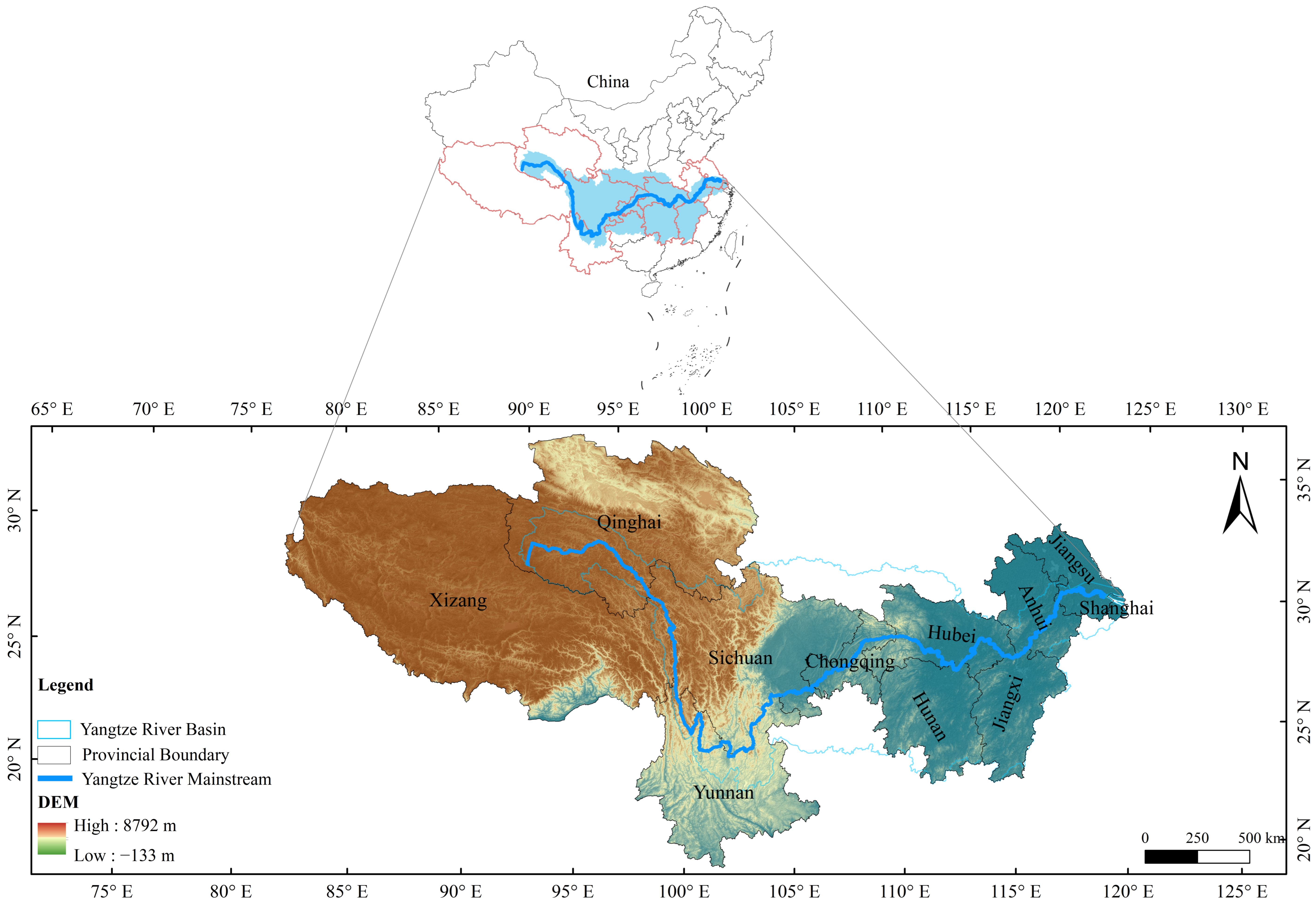
The Yangtze River Basin extends from the Qinghai–Xizang Plateau to the East China Sea and spans regions with contrasting climates, topography, ecological functions, and development levels. This study considers 11 provincial-level administrative regions commonly associated with the basin: Shanghai, Jiangsu, Anhui, Jiangxi, Hubei, Hunan, Chongqing, Sichuan, Yunnan, Xizang, and Qinghai (Figure 1). The lower reaches are highly urbanized and economically developed; the middle reaches contain major agricultural and manufacturing centers; and the upper reaches perform critical water-source conservation and ecological-barrier functions.

In recent years, annual water use in the Yangtze River Basin has exceeded 200 billion m³, with agricultural water use accounting for more than 50%. Industrial and domestic water demand has also continued to increase. Differences in resource endowments, development stages, industrial structures, urbanization processes, and water-resource management capacity have produced marked regional disparities in WRUE. The upper reaches are characterized by intensive hydropower development and important ecological functions, while parts of the middle and lower reaches face increasing pressures from industrial and domestic water demand. These regional contrasts provide a representative basis for examining the spatial differentiation and long-term evolution of WRUE.

It should be noted that the analytical units in this study are provincial-level administrative regions rather than hydrological sub-basins. For provinces whose administrative boundaries extend beyond the hydrological boundary of the Yangtze River Basin, province-wide statistical data were used because the socioeconomic, water-use, and environmental indicators required for the efficiency analysis are consistently reported at the provincial administrative level. Therefore, the spatial framework of this study represents provincial-level regions associated with the Yangtze River Basin rather than a strictly basin-clipped statistical system. This distinction is considered when interpreting the results.

2.2. Data and Processing

From an input–output perspective, an indicator system was selected to account for water resource inputs, economic outputs, and environmental constraints. In this study, WRUE is operationalized as an environmentally adjusted total-factor efficiency measure that jointly considers water, labor, and capital inputs, desirable economic output, and undesirable environmental output. The input indicators comprise total regional water use, year-end employment, and capital stock, representing water, labor, and capital inputs, respectively. Gross domestic product (GDP) was selected as the desirable output to represent economic output. Chemical oxygen demand (COD) emissions were selected as the representative undesirable output to characterize the environmental pollution pressure associated with water use. As a widely reported indicator of organic pollution load, COD provides relatively broad provincial coverage and a comparatively long time series over the study period. Other potential water-pollution indicators, including biochemical oxygen demand (BOD) and other pollutant measures, were not incorporated because the temporal and spatial coverage of their annual provincial-level data was insufficient to construct a comparable panel covering all study regions throughout the entire study period. Accordingly, COD was retained as the representative undesirable output to maintain the temporal continuity and cross-regional comparability of the panel dataset (see

Table 1. Input–output indicator system.

Indicator Type	Indicator	Unit	Data Source
Input	Total regional water use	108 m3	China Water Resources Bulletin
	Capital stock	CNY 108	China Statistical Yearbook; China City Statistical Yearbook
	Employment at year-end	104 persons	China Statistical Yearbook
Desirable output	GDP	CNY 108	China Statistical Yearbook
Undesirable output	COD emissions	104 t	China Statistical Yearbook; Water Resources Bulletin of the Yangtze River Basin and Rivers of Southwest China

Note: CNY denotes Chinese yuan. Capital stock and GDP are expressed at constant 2010 prices.

).

To examine the factors associated with the spatial differentiation of WRUE, 11 factors were selected across six dimensions: water-use structure, economic development, industrial structure, urban development, technological innovation and education, and environmental governance. Continuous explanatory variables were discretized prior to the GeoDetector analysis. The number of strata adopted for each variable is reported in

Table 2. Explanatory factors examined for the spatial differentiation of water resource use efficiency in the Yangtze River Basin.

Dimension	Influencing Factor	Code	Number of Classes
Water-use structure	Share of industrial water use	$X_1$	3
	Per capita water use	$X_2$	5
Economic development	Water use per CNY 10,000 of GDP	$X_3$	5
	GDP per capita	$X_4$	5
Industrial structure	Share of the primary industry	$X_5$	3
Urban development	Urban population density	$X_6$	5
	Urbanization rate at year-end	$X_7$	3
	Total imports and exports	$X_8$	5
Technological innovation and education	Share of science and technology expenditure in total fiscal expenditure	$X_9$	5
	Students enrolled in higher education institutions per 100,000 population	$X_{10}$	3
Environmental governance	Daily wastewater treatment volume	$X_{11}$	5

. The classification thresholds were derived from the pooled observations over the complete 2010–2024 period and were subsequently held fixed across the three subperiods to ensure temporal comparability.

The data were obtained from the China Statistical Yearbook, China City Statistical Yearbook, China Water Resources Bulletin, Water Resources Bulletin of the Yangtze River Basin and Rivers of Southwest China, and the statistical yearbooks, statistical bulletins, and water-resources bulletins of the 11 provincial-level administrative regions. Capital stock was estimated using the method proposed by Shan [23]. Capital stock and GDP were deflated to constant 2010 prices. Because the fixed-asset investment price index was discontinued after 2020, the consumer price index of each provincial-level administrative region was used as a substitute. Changes in the statistical reporting scope of COD emissions resulted in gaps in directly comparable observations for Qinghai, Xizang, Chongqing, Hunan, Hubei, Jiangxi, and Anhui in 2018 and 2019, corresponding to 14 province-year observations. These observations accounted for 8.5% of the COD series (14 of 165 observations) and approximately 1.7% of all observations across the five DEA input–output indicators (14 of 825 observations). To maintain the continuity of the panel dataset, the missing COD values were estimated using the TREND function in Microsoft Excel, which fits a least-squares linear trend to the available annual COD time series for each affected region. No imputation was applied to the remaining input or output indicators. The study period ends in 2024 because a complete and harmonized 2025 panel for all input–output and explanatory indicators was not available at the time of revision.

2.3. Methods

The analytical framework was organized around three linked questions: what is the spatiotemporal pattern of WRUE, what factors are associated with its spatial differentiation, and how do efficiency states evolve over time under different neighborhood conditions? The super-efficiency SBM-window DEA model provides comparable WRUE estimates across provincial-level regions and years, allowing the temporal and spatial pattern of efficiency to be identified. Changes in productivity are further examined using the ML index, which separates the contributions of technological change and efficiency change. GeoDetector 2015 (Excel-based version) is used to assess which factors, individually and in combination, are most strongly associated with the spatial differentiation of WRUE. The Markov analysis focuses on the evolutionary process itself: the conventional Markov chain characterizes state persistence and transition probabilities, whereas the spatial Markov chain evaluates how these probabilities vary under different geographic neighborhood conditions. Steady-state distributions are derived from the estimated transition matrices to describe the long-term tendencies implied by the observed transition structure.

2.3.1. Super-Efficiency SBM Model

This study employs the super-efficiency SBM model incorporating undesirable outputs, based on the models developed and subsequently extended by Tone [24,25]. The model extends the conventional DEA framework by incorporating input and output slack variables and constraints on undesirable outputs. It allows efficiency scores to exceed unity, thereby enabling further differentiation and ranking among efficient decision-making units (DMUs). This study employs a non-oriented super-efficiency SBM model incorporating undesirable outputs under the assumption of constant returns to scale (CRS), which is adopted to assess provincial WRUE relative to a common production frontier and thereby maintain consistency in cross-regional efficiency comparisons. COD emissions were directly incorporated as an undesirable output without reciprocal, translation, or other directional transformations, and all input and output observations are strictly positive. The model is formulated as follows:

$${\rho }^{*} = \min {\displaystyle \frac{\frac{1}{n}{\displaystyle {\sum }_{i=1}^n}\frac{{\overline{x}}_i}{x_{i_0}}}{\frac{1}{{\partial }_1+{\partial }_2}\left({\displaystyle {\sum }_{r=1}^{{\partial }_1}}\frac{{\overline{y}}_r^a}{{\overline{y}}_{r_0}^a}+{\displaystyle {\sum }_{l=1}^{{\partial }_2}}\frac{{\overline{y}}_l^b}{{\overline{y}}_{l_0}^b}\right)}},\hspace{1em}\text{s.t.}\left\{\begin{array}{l}\overline{x} \ge {\displaystyle \sum _{j=1, j\ne 0}^n}{\mathsf{\lambda }}_j{x}_j,\\ {\overline{y}}^a \le {\displaystyle \sum _{j=1, j\ne 0}^n}{\mathsf{\lambda }}_j{y}_j^{ a},\\ {\overline{y}}^{b } \ge {\displaystyle \sum _{j=1, j\ne 0}^n}{\mathsf{\lambda }}_j{y}_j^b,\\ \overline{x} \ge x_0, {\overline{y}}^a \le y_0^a, {\overline{y}}^{b } \ge y_0^{ b}\end{array}\right.$$

(1)

In the equation, ${\rho }^{*}$ represents the water resource use efficiency of the Yangtze River Basin. $x$, $y^a$, and $y^b$ denote the inputs, desirable outputs, and undesirable outputs, respectively. ${\overline{x}}_i$, ${\overline{y}}_r^a$, and ${\overline{y}}_l^b$ represent the slack variables of the inputs, desirable outputs, and undesirable outputs, respectively. $\lambda$ is the nonnegative intensity vector, and the adjusted desirable and undesirable outputs are constrained to be nonnegative. $n$, ${\partial }_1$, and ${\partial }_2$ denote the numbers of input, desirable-output, and undesirable-output indicators, respectively. $x_{i_0}$, ${\overline{y}}_{r_0}^a$, and ${\overline{y}}_{l_0}^b$ represent the adjusted values of the inputs, desirable outputs, and undesirable outputs, respectively.

To improve the temporal comparability of the efficiency estimates, this study combines the super-efficiency SBM model with the window DEA method. Window DEA treats observations of the same province in different years as relatively independent evaluation units and constructs reference sets through rolling windows [10]. Let $T$ denote the number of years in the study period and $d$ denote the window width. The number of windows, $L$, is calculated as follows:

$$L=T-d+1.$$

The study period extends from 2010 to 2024, covering 15 years. A three-year window width was adopted as the baseline specification. Given the 11 provincial-level regions, each three-year window contains 33 province-year DMUs, providing a sufficiently broad reference set while preserving sensitivity to short-term efficiency changes. In comparison, a two-year window provides a smaller reference set and may be more sensitive to year-specific fluctuations, whereas four- or five-year windows may smooth short-term temporal variation. The three-year window therefore represents a reasonable compromise between reference-set stability and temporal resolution. For the same province-year observation appearing in different windows, the arithmetic mean of its efficiency scores was calculated as the final efficiency score for that year.

To assess the sensitivity of the results to this specification, the model was re-estimated using two-, four-, and five-year windows, with all other model settings, input–output indicators, data-processing procedures, and aggregation rules kept unchanged. The corresponding sensitivity results are reported in Supplementary Table S1.

2.3.2. Malmquist–Luenberger Index

The super-efficiency SBM model can only measure the relative efficiency of each decision-making unit in a specific year. To reveal the underlying sources of efficiency changes, this study introduces the ML index model [26]. The model is constructed using directional distance functions (DDFs) [27], with the direction vector specified as $g=\left(-x,y^a,-y^b\right.$). Accordingly, the ML index of water resource use efficiency in the Yangtze River Basin from period $t$ to period $t+1$ is defined as follows:

$$M{L}_t^{t+1}={\left[{\displaystyle \frac{1+D_t\left(x_t,y_t^a,y_t^b;g\right)}{1+D_t\left(x_{t+1},y_{t+1}^a,y_{t+1}^b;g\right)}}\times {\displaystyle \frac{1+D_{t+1}\left(x_t,y_t^a,y_t^b;g\right)}{1+D_{t+1}\left(x_{t+1},y_{t+1}^a,y_{t+1}^b;g\right)}}\right]}^{1/2}$$

(2)

The ML index can be decomposed as $ML=EC\times TC$, while $EC$ can be further decomposed as $EC=PEC\times SEC$. In the above equation, $D_t\left(x_t,y_t^a,y_t^b;g\right)$ and $D_{t+1}\left(x_t,y_t^a,y_t^b;g\right)$ denote the directional distance functions of the observation in period t evaluated relative to the production technology sets in periods $t$ and $t+1$, respectively. Similarly, $D_t\left(x_{t+1},y_{t+1}^a,y_{t+1}^b;g\right)$ and $D_{t+1}\left(x_{t+1},y_{t+1}^a,y_{t+1}^b;g\right)$ denote the directional distance functions of the observation in period t + 1 evaluated relative to the production technology sets in periods $t$ and $t+1$, respectively. An ML index greater than 1 indicates an increase in total factor productivity, whereas a value below 1 indicates a decline. $EC$ denotes efficiency change, reflecting changes in technical efficiency, and $TC$ denotes technological change. $PEC$ and $SEC$ represent pure technical efficiency change and scale efficiency change, respectively.

2.3.3. GeoDetector

To identify the dominant factors underlying the spatial differentiation of water resource use efficiency (WRUE) in the Yangtze River Basin, this study employs the factor detector and interaction detector of the GeoDetector model [20]. The factor detector measures the explanatory power of a given influencing factor for the spatial differentiation of WRUE. The q-statistic is expressed as follows:

$$q=1-{\displaystyle \frac{1}{N{\sigma }^2}}{\displaystyle \sum _{h=1}^L}{N}_h{\sigma }_h^2$$

(3)

where $q$ denotes the explanatory power of the detected factor for the spatial differentiation of WRUE and ranges from 0 to 1; $h$ denotes the stratum, and $L$ is the total number of strata; $N_h$ and ${\sigma }_h^2$ represent the number of samples and the variance of WRUE within stratum $h$, respectively; and $N$ and ${\sigma }^2$ denote the total number of samples and the overall variance of WRUE, respectively. A larger $q$-value indicates greater explanatory power of the corresponding factor for the spatial differentiation of WRUE.

Under the baseline specification, continuous explanatory variables were discretized using a factor-specific classification scheme. Variables assigned three strata were classified using K-means clustering, whereas variables assigned five strata were classified using the natural breaks method. The number of strata adopted for each factor is reported in Table 2. To ensure temporal comparability, the classification rules were derived from the pooled observations for 2010–2024 and then held fixed across the three subperiods.

The interaction detector is further used to compare the joint explanatory power of two factors with their individual explanatory power by comparing $q\left(X_i\cap X_j\right)$ with $q\left(X_i\right)$ and $q\left(X_j\right)$. When $q\left(X_i\cap X_j\right)$ exceeds the larger of the two individual $q$-values, the interaction is classified as bivariate enhancement; when it exceeds the sum of the two individual $q$-values, it is classified as nonlinear enhancement. Conversely, an interaction value lower than the individual $q$-values indicates reduced explanatory power under joint stratification.

To assess the robustness of the GeoDetector results to discretization settings, two complementary sensitivity analyses were conducted. First, equal-interval and quantile classifications were applied while retaining the factor-specific number of strata used in the baseline specification. Second, the discretization method was fixed as quantile classification, and the number of strata was varied systematically from three to four and five for all factors. In all cases, classification thresholds were derived from the pooled observations for 2010–2024 and held fixed across the three subperiods. The resulting q-values and factor rankings were compared with the baseline results. Detailed results are provided in Supplementary Tables S2 and S3.

2.3.4. Markov Chain

The conventional Markov chain model characterizes the evolutionary process of objects among different states based on their initial-state probabilities and inter-state transition probabilities [28]. To examine the transition patterns of WRUE, the efficiency values are classified into three categories—low, medium, and high efficiency—using the quantile method, and these categories are assigned state numbers 1, 2, and 3, respectively. The probability that the WRUE of a province transitions from state $E_i$ in year t to state $E_j$ in year t + 1 is calculated as follows:

$$P_{ij}\left(E_i\to E_j\right)={\displaystyle \frac{n_{ij}}{n_i}}$$

(4)

where $P_{ij}$ denotes the probability that the WRUE of a province transitions from state $E_i$ to state $E_j$; $n_{ij}$ represents the number of observations that are in state $i$ in year $t$ and transition to state $j$ in year $t+1$; and $n_i$ denotes the total number of observations in efficiency state $i$ in year $t$. When WRUE is divided into $N$ states, an $N\times N$ transition probability matrix is obtained. In this study, $N=3$; therefore, the resulting transition probability matrix is a $3\times 3$ matrix, as shown in

Table 3. Markov transition probability matrix ($N$ = 3).

t/(t + 1)	1	2	3
1	P11	P12	P13
2	P21	P22	P23
3	P31	P32	P33

.

The spatial Markov chain model extends the conventional Markov chain model by incorporating a spatial lag condition [29]. It is used to examine whether the state-transition probabilities of a target region vary under different efficiency conditions of geographically adjacent regions. The spatial lag value is calculated as follows:

$${\mathrm{L}\mathrm{a}\mathrm{g}}_i={\displaystyle \sum _{j=1}^n}{W}_{ij}{Y}_j$$

(5)

where $Y_j$ denotes the observed value of region $j$; $W_{ij}$ is an element of the spatial weight matrix and represents the spatial relationship between regions $i$ and $j$; ${\mathrm{L}\mathrm{a}\mathrm{g}}_i$ denotes the spatial lag value of region $i$; and $n$ is the total number of regions. This study employs a binary contiguity-based spatial weight matrix, in which $W_{ij}=1$ if regions $i$ and $j$ are adjacent and $W_{ij}=0$ otherwise. Accordingly, the spatial lag used in this study represents the efficiency context of geographically adjacent provincial-level regions and is intended to characterize local geographic neighborhood conditions.

By incorporating the spatial weight matrix, the conventional $N\times N$ transition probability matrix is extended into a set of conditional transition probability matrices with an $N\times N\times K$ structure:

$$P^{\left(k\right)}=\left[\begin{array}{cccc}{P}_{11\mid k}& P_{12\mid k}& \dots & P_{1N\mid k}\\ P_{21\mid k}& P_{22\mid k}& \dots & P_{2N\mid k}\\ ⋮& ⋮& \ddots & ⋮\\ P_{N1\mid k}& P_{N2\mid k}& \dots & P_{NN\mid k}\end{array}\right],k=1,2,\dots ,K$$

(6)

where $P_{ij\mid k}$ denotes the conditional probability that WRUE transitions from state $i$ to state $j$ under spatial lag type $k$, and $K$ is the number of spatial lag categories.

As the number of state transitions increases, the state distribution gradually converges to a stable distribution. The probabilities associated with the respective states are referred to as the limiting distribution or steady-state probabilities. To characterize the long-term distribution implied by the estimated WRUE transitions, the steady-state distribution of the transition matrix must therefore be determined. If the Markov chain satisfies the ergodicity condition, a unique limiting distribution vector ${\pi }^{\left(k\right)}$ exists for each spatial lag type $k$ and satisfies the following equilibrium conditions:

$$\begin{gathered} {\pi }^{\left(k\right)}={\pi }^{\left(k\right)}{P}^{\left(k\right)},k=1,2,\dots ,K \\ \text{s.t.} \left\{\begin{array}{c}{\pi }_j^{\left(k\right)}={\displaystyle \sum _{i=1}^N}{\pi }_i^{\left(k\right)}{p}_{ij\mid k},j=1,2,\dots ,N,\\ {\displaystyle \sum _{j=1}^N}{\pi }_j^{\left(k\right)}=1,\\ 0\le {\pi }_j^{\left(k\right)}\le 1.\end{array}\right. \end{gathered}$$

(7)

where ${\pi }^{\left(k\right)}$ denotes the limiting state distribution vector under spatial lag type $k$, and ${\pi }_j^{\left(k\right)}$ represents the steady-state probability that the system remains in WRUE state $j$ in the long run.

To mitigate the instability of probability estimates caused by sparse transition counts in finite samples, following Kang and Rey [30], we applied an ordered discrete product-kernel method to smooth the transition probabilities of both the conventional and spatial Markov chains.

3. Results

3.1. Spatiotemporal Evolution of WRUE in the Yangtze River Basin

3.1.1. Temporal Evolution

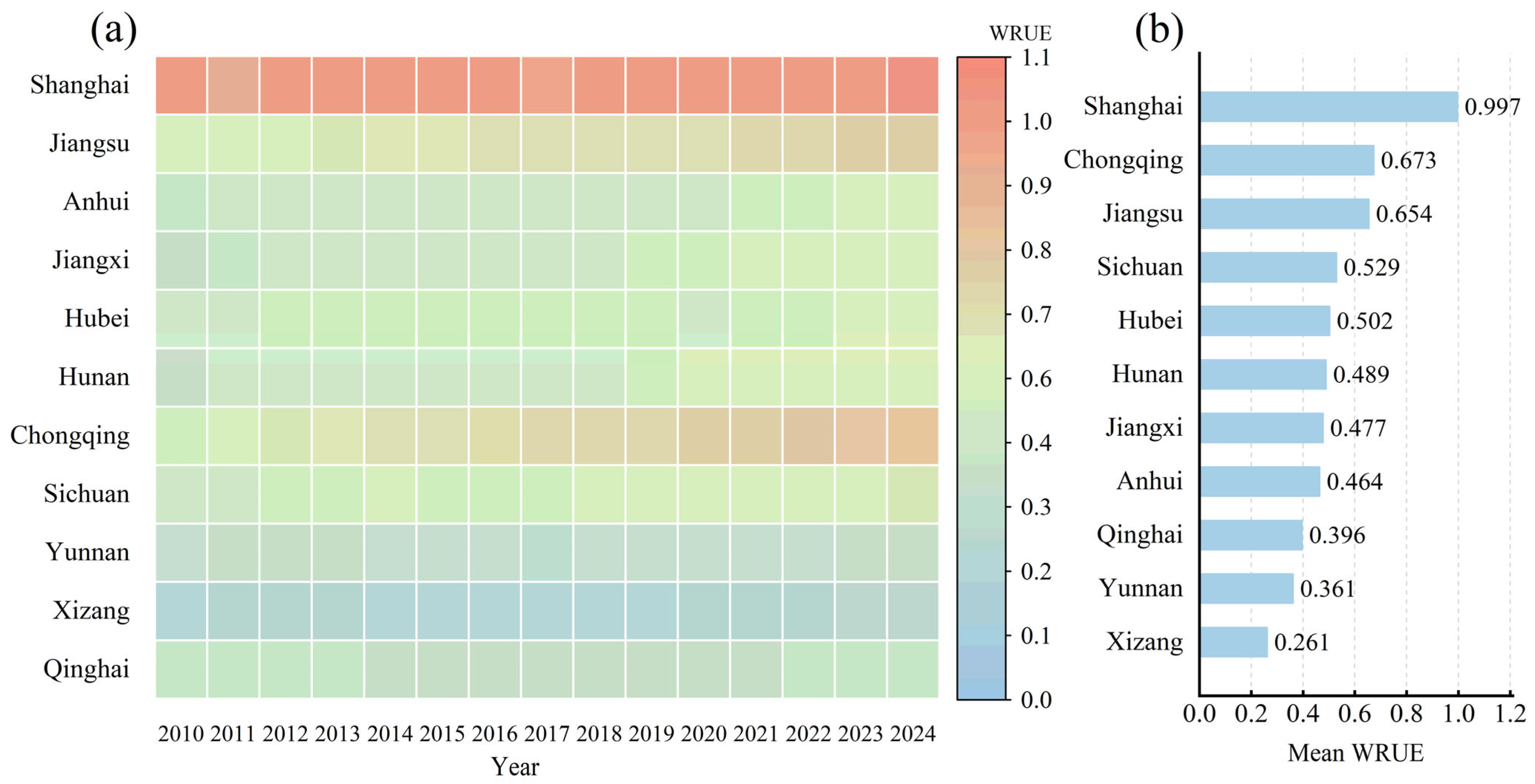
From a temporal perspective, WRUE across the 11 provincial-level regions of the Yangtze River Basin exhibited an overall fluctuating upward trend from 2010 to 2024, accompanied by persistent interregional differences. Figure 2a shows the annual variation in WRUE across the study regions. Shanghai, Chongqing, and Jiangsu generally maintained relatively high WRUE levels, with Shanghai recording values above 1 in several years and remaining among the highest-performing regions throughout the study period. Sichuan, Hubei, Hunan, Jiangxi, and Anhui were concentrated at intermediate levels and generally showed gradual improvement. Qinghai, Yunnan, and Xizang remained at comparatively low levels, although modest increases were observed in some years.

Figure 2b presents the multiyear mean WRUE values and corresponding rankings of the 11 regions. Shanghai recorded the highest mean WRUE of 0.997, followed by Chongqing at 0.673 and Jiangsu at 0.654. Xizang had the lowest mean value of 0.261, while Yunnan and Qinghai also remained among the lower-ranked regions. These results indicate that substantial interregional disparities persisted despite the overall improvement in WRUE during 2010–2024.

The window-width sensitivity analysis showed that the main WRUE patterns remained stable across alternative specifications. Provincial rankings were identical under the two-, three-, four-, and five-year windows, with Spearman rank correlations of 1.000 between each alternative specification and the baseline three-year window. Relative to the baseline, the mean absolute differences in provincial mean WRUE were 0.0086, 0.0060, and 0.0096 for the two-, four-, and five-year windows, respectively. The spatial ordering of the lower reaches > middle reaches > upper reaches was preserved under all window specifications. These results indicate that the principal WRUE findings are robust to reasonable changes in window width (Supplementary Table S1).

3.1.2. Spatial Evolution

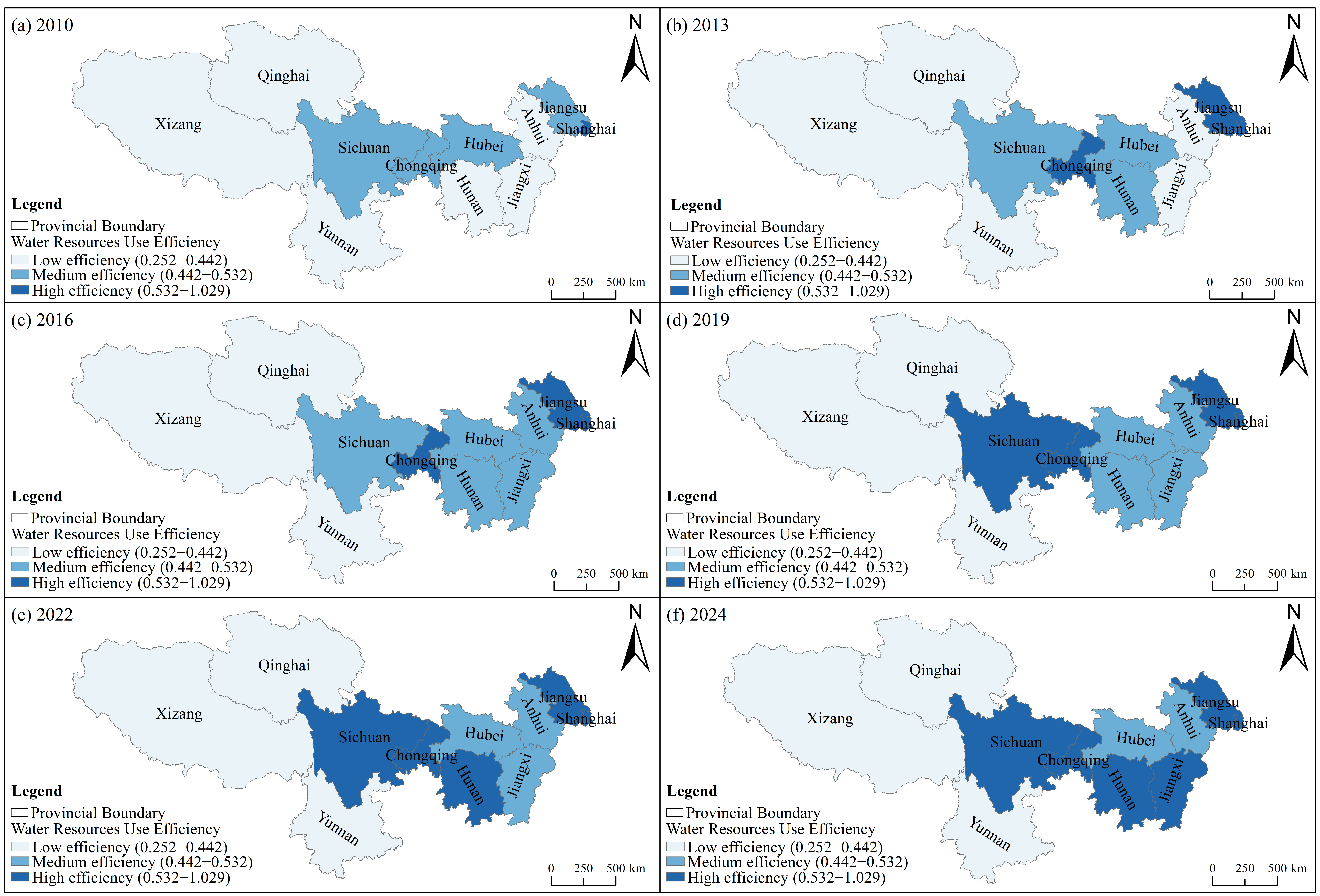
Figure 3a–f present the spatial distribution of WRUE in 2010, 2013, 2016, 2019, 2022, and 2024, respectively. A common set of quantile-based classification thresholds was applied to all six years to ensure direct temporal comparability. The maps show persistent spatial heterogeneity among the provincial-level regions. Relatively high WRUE values were generally concentrated in the lower reaches, intermediate values occurred more frequently in the middle reaches, and comparatively low values were mainly observed in parts of the upper reaches.

This spatial ordering is also reflected in the multiyear regional averages. The lower reaches recorded the highest mean WRUE of 0.705, followed by the middle reaches at 0.489 and the upper reaches at 0.444. Shanghai and Jiangsu consistently occupied relatively high-efficiency positions, while Chongqing also showed comparatively high WRUE among the upper-reach regions. Qinghai, Yunnan, and Xizang remained at relatively low efficiency levels during much of the study period. Although WRUE changed across individual regions over time, the broader spatial gradient from the lower reaches to the middle and upper reaches remained evident throughout the study period.

3.2. Productivity Change and Factors Associated with Spatial Differentiation

3.2.1. Structural Decomposition of Efficiency Evolution

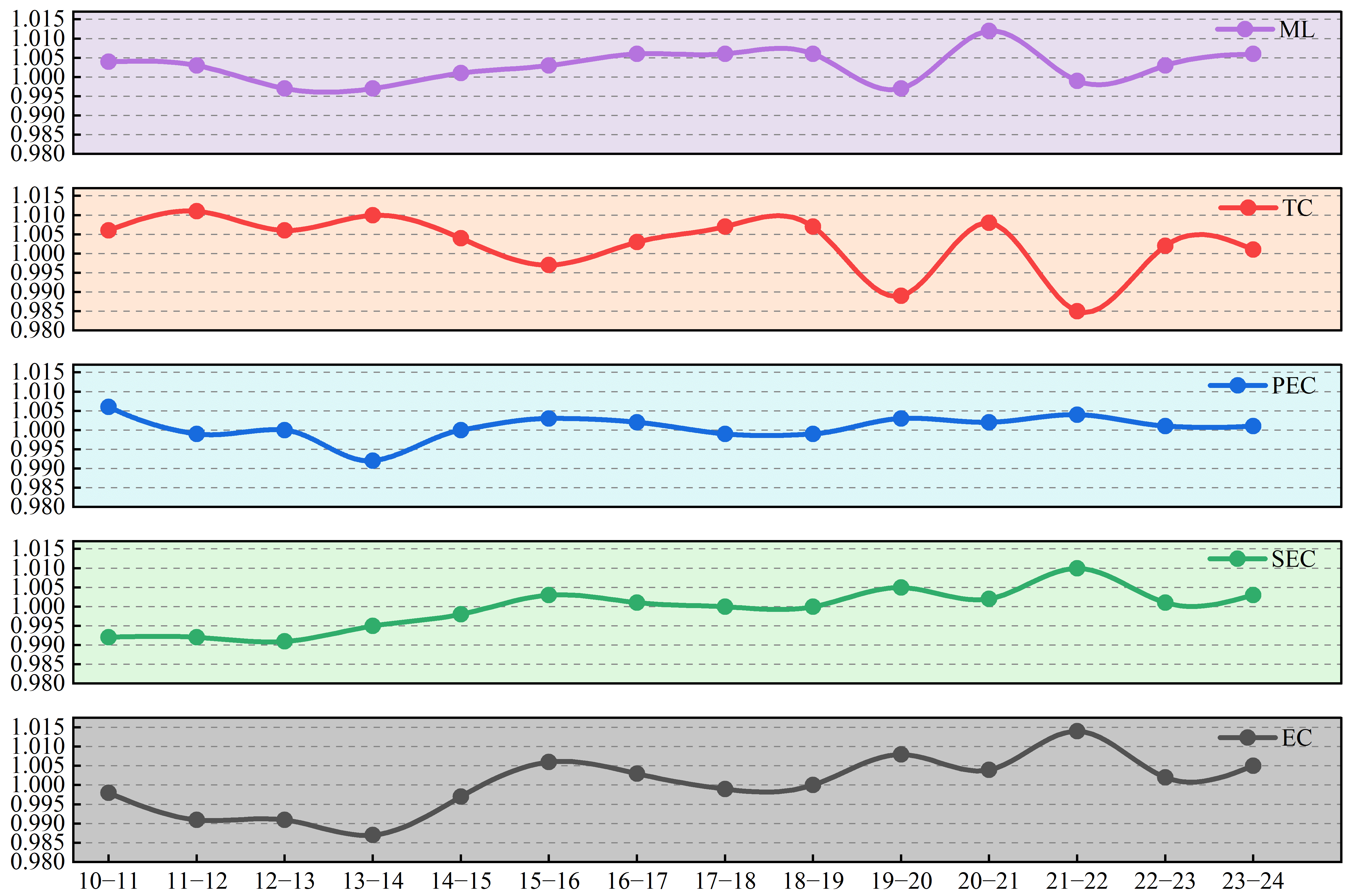
The ML index was used to measure and decompose changes in total factor productivity across the provincial-level administrative regions of the Yangtze River Basin, and the results are presented in Figure 4. The ML index for WRUE fluctuated around the threshold value of 1, with a multiyear mean of 1.004, indicating a modest overall improvement in the total factor productivity of water resource use from 2010 to 2024.

In most years, technological change (TC) made the largest contribution to fluctuations in the ML index, whereas efficiency change (EC), particularly its scale efficiency change (SEC) component, also contributed during certain years. Pure technical efficiency change (PEC) fluctuated markedly during the early study period and generally exceeded SEC. It gradually stabilized in the later period and was subsequently surpassed by SEC. Overall, the relative contributions of these components indicate a gradual shift from the predominance of TC toward a more combined contribution of technological change, technical efficiency improvement, and scale optimization. During 2021–2022, TC declined, whereas EC and SEC increased markedly, indicating that improvements in technical efficiency, particularly scale efficiency, partially offset the weakened contribution of technological change to the ML index.

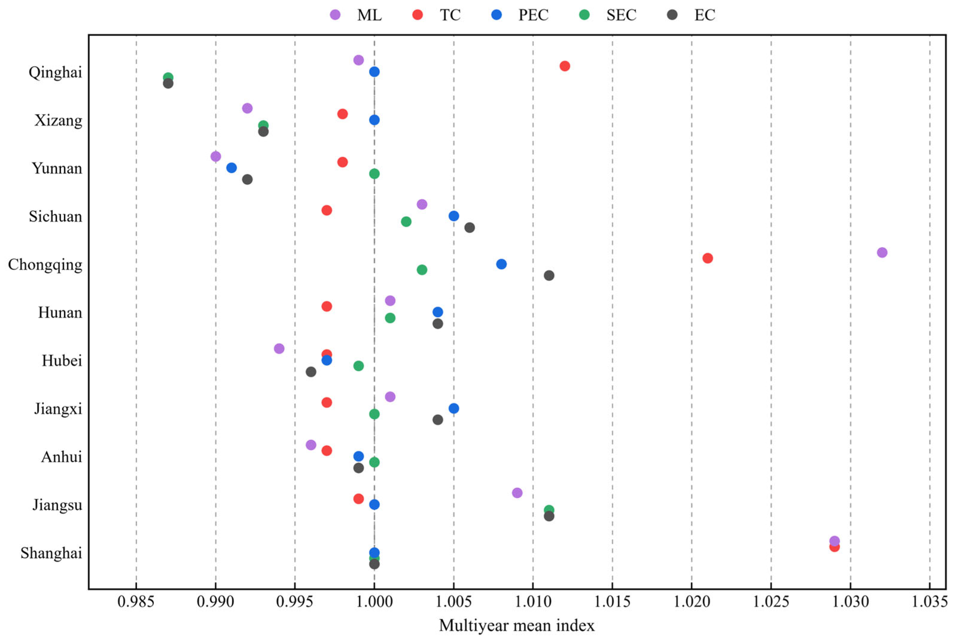
The multiyear mean ML index and its decomposition components for the 11 provincial-level administrative regions of the Yangtze River Basin are presented in Figure 5. Clear regional differences were observed in the ML index and its components. Shanghai and Chongqing recorded relatively high ML values. Shanghai also exhibited a comparatively high TC value, whereas Chongqing showed relatively high values of both TC and EC. Jiangsu had a comparatively high SEC value. In several regions of the middle and upper reaches, the ML index and most of its decomposition components remained close to 1, indicating relatively limited interannual changes in total-factor water resource productivity. Overall, the relative contributions of TC, EC, PEC, and SEC varied across regions, revealing spatial heterogeneity in the composition of productivity change.

3.2.2. Factors Associated with Spatial Differentiation

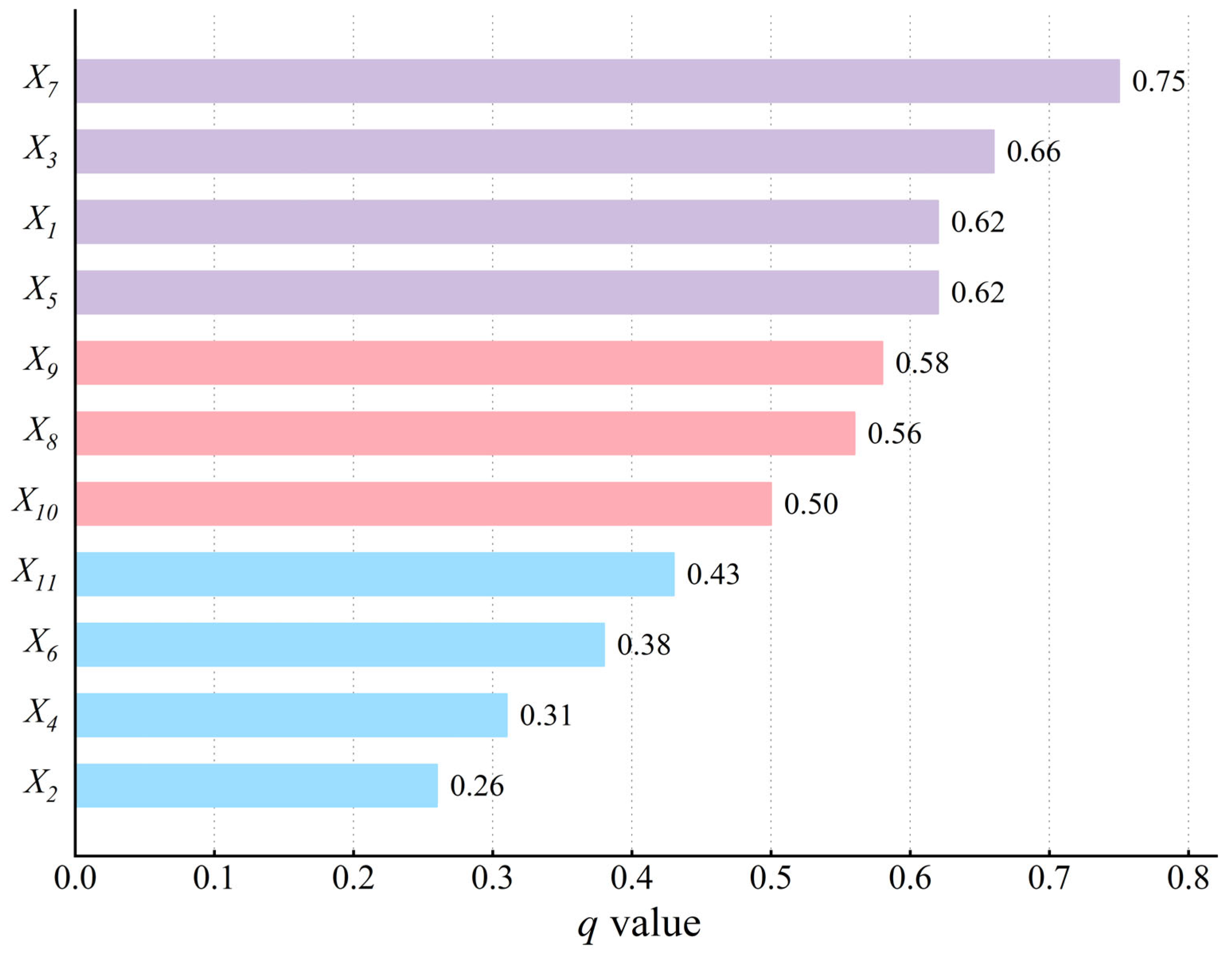
The factor detector results showed significant differences in the explanatory power of the selected socioeconomic and water-use factors for the spatial differentiation of WRUE (Figure 6). Among the 11 factors, the year-end urbanization rate ($X_7$) exhibited the highest q-value (0.75), followed by water use per CNY 10,000 of GDP ($X_3$), the industrial water-use share ($X_1$), and the primary-industry share ($X_5$), with q-values of 0.66, 0.62, and 0.62, respectively. These four factors therefore exhibited relatively high explanatory power under the baseline specification.

Several other factors also showed moderate explanatory power. The share of science and technology expenditure in total fiscal expenditure ($X_9$), total imports and exports ($X_8$), and higher education enrollment per 100,000 population ($X_{10}$) had q-values of approximately 0.50–0.58. Daily wastewater treatment volume ($X_{11}$), urban population density ($X_6$), GDP per capita ($X_4$), and per capita water use $(X_2$) showed comparatively lower explanatory power. In particular, $X_2$ had the lowest q-value among the selected factors, indicating relatively weak explanatory power when considered individually.

Overall, the factor-detector results indicate that the spatial differentiation of WRUE is associated with multiple dimensions of urban development, water-use intensity and structure, industrial composition, technological and educational conditions, and environmental governance, although the magnitude of their explanatory power differs substantially.

Table 4. Stage-specific factor detector results for the spatial differentiation of WRUE in the Yangtze River Basin.

2010–2014		2015–2019		2020–2024
Core Factor	$\mathit{q}$-Value	Core Factor	$\mathit{q}$-Value	Core Factor	$\mathit{q}$-Value
$X_1$	0.651 ***	$X_1$	0.786 ***	$X_1$	0.698 ***
$X_3$	0.776 ***	$X_3$	0.686 ***	$X_3$	0.686 ***
$X_5$	0.770 ***	$X_5$	0.570 ***	$X_5$	0.568 ***
$X_7$	0.858 ***	$X_7$	0.711 ***	$X_7$	0.773 ***

Note: *** p < 0.001. Values without asterisks are not statistically significant at the 5% level.

presents the stage-specific explanatory power of the four factors that exhibited relatively high q-values in the baseline analysis. The results show that their relative explanatory power varied across the three subperiods. The urbanization rate ($X_7$) maintained relatively high explanatory power throughout the study period, with q-values of 0.858, 0.711, and 0.773 in 2010–2014, 2015–2019, and 2020–2024, respectively. The explanatory power of the industrial water-use share ($X_1$) increased from 0.651 in the first period to 0.786 in 2015–2019 and subsequently decreased to 0.698. Water use per CNY 10,000 of GDP ($X_3$) decreased from 0.776 to approximately 0.686 and then remained nearly unchanged, whereas the primary-industry share ($X_5$) decreased from 0.770 to approximately 0.57 in the latter two periods. All four factors remained statistically significant across the three subperiods. Overall, these results indicate temporal variation in the relative explanatory power of the major factors associated with the spatial differentiation of WRUE.

The robustness analyses showed that changes in the discretization method and the number of strata affected the absolute q-values and relative rankings of some factors, indicating that the GeoDetector results were not completely invariant to discretization settings. Nevertheless, the broader ranking structure remained generally comparable. Under quantile classification, the Spearman rank correlations between the baseline ranking and the rankings obtained using three, four, and five strata were 0.745, 0.855, and 0.873, respectively. The rankings obtained using four and five strata were particularly similar ($\rho =0.991$). These results indicate a substantial, although not complete, degree of consistency in the overall factor structure. Detailed results are provided in Tables S2 and S3.

Some factor-specific differences were also observed. Water use per CNY 10,000 of GDP ($X_3$) remained among the higher-ranking factors when the number of quantile strata was varied, ranking third, fourth, and third under the three-, four-, and five-strata specifications, respectively. Its q-value under five-strata quantile classification (0.649) was also close to the baseline value (0.660). In contrast, its q-value decreased to 0.236 under equal-interval classification. The equal-interval scheme produced highly unbalanced strata for $X_3$, suggesting that its lower q-value was partly associated with the skewed distribution of this variable. Accordingly, the explanatory power of $X_3$ is interpreted with greater caution than that of factors showing greater consistency across discretization settings.

3.2.3. Interaction Detection of Explanatory Factors

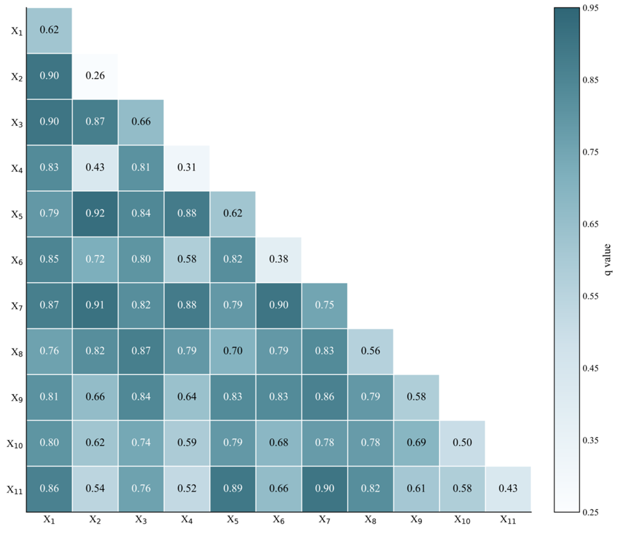
The interaction detector results showed that the q values of all pairwise interactions were higher than those of the corresponding individual factors (Figure 7), indicating that joint factor stratification provided greater explanatory power for the spatial differentiation of WRUE than individual-factor stratification. The strongest interaction was observed between per capita water use ($X_2$) and the primary-industry share ($X_5$), with a q value of 0.92, followed by the interaction between per capita water use ($X_2$) and the urbanization rate ($X_7$), with a q value of 0.91. The interactions of $X_1\cap X_2$, $X_1\cap X_3$, $X_6\cap X_7$, and $X_7\cap X_{11}$ all reached 0.90. Notably, although per capita water use had relatively low explanatory power individually (q = 0.26), its joint stratification with the primary-industry share and urbanization rate yielded substantially higher q-values. These results indicate that combinations of water-use patterns, industrial structure, urban development, and environmental governance provide greater explanatory power for the spatial differentiation of WRUE than the corresponding individual factors.

3.3. State Transitions and Long-Term Evolution of WRUE

3.3.1. State Transition Characteristics Based on the Conventional Markov Chain Model

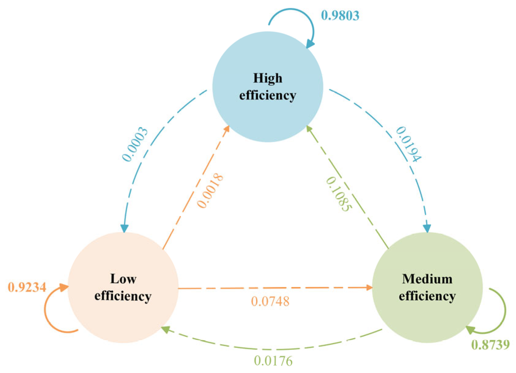
A WRUE state-transition probability matrix was constructed using the conventional Markov chain method. The results show the following. The transition probabilities are shown in Figure 8.

• The probabilities that the low-, medium-, and high-efficiency states remained unchanged in the subsequent period were 92.34%, 87.39%, and 98.03%, respectively. These probabilities were markedly higher than those of transitions to other states, indicating strong path dependence and persistence in the efficiency states of the provincial-level regions.
• The probability of a direct transition from the low- to the high-efficiency state was only 0.18%, whereas the probability of transitioning from the medium- to the high-efficiency state was 10.85%. These results indicate that efficiency upgrading generally occurs through stepwise transitions.
• The low- and high-efficiency states exhibited relatively greater stability, indicating a certain degree of stratified clustering across different efficiency levels.

3.3.2. State Transitions Under Different Spatial Neighborhood Conditions

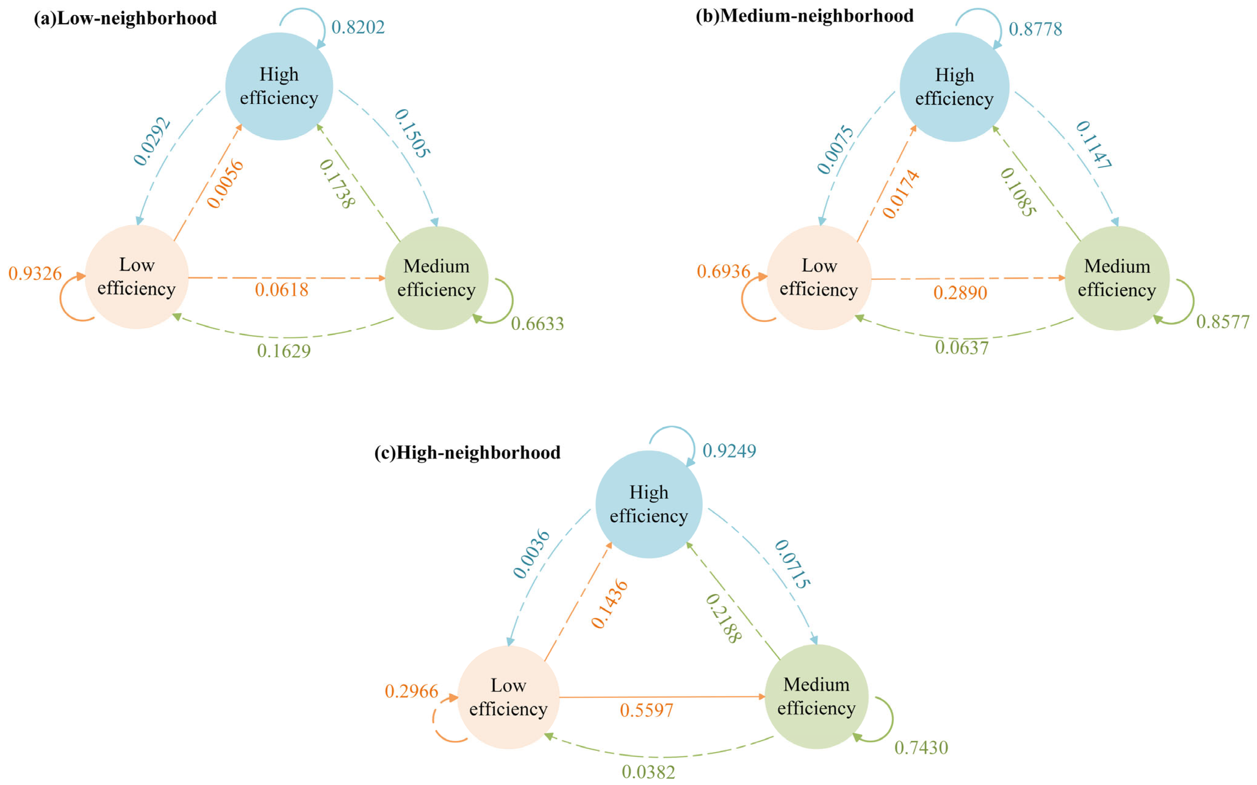
Spatial lag conditions were incorporated into the conventional Markov chain to construct a spatial Markov transition probability matrix for WRUE. The spatial Markov transition probabilities are shown in Figure 9.

• After spatial neighborhood conditions were introduced, the transition probabilities of all efficiency states changed markedly. For example, the probability of a medium-efficiency region transitioning to the high-efficiency state was 10.85% in the conventional transition matrix. Under low- and high-efficiency neighborhood conditions, this probability increased to 17.38% and 21.88%, respectively. These results indicate that the transition probabilities of efficiency states vary across different spatial neighborhood conditions.
• Neighborhood effects differed across initial efficiency states. For low-efficiency regions, the probability of transitioning to the medium-efficiency state decreased from 7.48% to 6.18% under low-efficiency neighborhood conditions. Under high-efficiency neighborhood conditions, the probability of directly transitioning to the high-efficiency state increased from 0.18% to 14.36%. This finding indicates that low-efficiency regions in high-efficiency neighborhoods exhibit a higher probability of upward transition.
• Low- and high-efficiency states remained highly stable within neighborhoods of the corresponding efficiency level. This result indicates that stratified clustering of efficiency states is more pronounced under certain spatial neighborhood conditions.

3.3.3. Long-Term Transition Tendencies and Steady-State Distribution

The steady-state distributions were derived from the transition probability matrices of the conventional and spatial Markov chain models, and the results are presented in

Table 5. Initial and steady-state distributions of WRUE in the Yangtze River Basin based on transition probabilities for 2010–2024.

Distribution Type	Spatial Neighborhood Type	State 1	State 2	State 3
Initial distribution		0.6364	0.2727	0.0909
Steady-state distribution without spatial lag effects		0.0371	0.1474	0.8155
Steady-state distribution with spatial lag effects	1	0.5830	0.2028	0.2142
	2	0.1181	0.5265	0.3554
	3	0.0170	0.2430	0.7400

. Compared with the initial distribution, the steady-state distribution without spatial effects shows marked decreases in the probabilities of states 1 and 2, whereas the probability of state 3 increases to 0.8155. This result indicates that, provided that the historical transition probabilities remain stable, the long-term distribution tends to shift toward higher efficiency states.

After spatial lag conditions are incorporated, the steady-state distributions differ markedly across neighborhood types. Under neighborhood type 1, the steady-state probability of the low-efficiency state remains as high as 58.30%, indicating a relatively high persistence probability of the low-efficiency state under low-efficiency neighborhood conditions. Under neighborhood type 2, the medium-efficiency state has the highest steady-state probability of 52.65%, while the probability of the high-efficiency state reaches 35.54%. This finding suggests that the medium-efficiency state remains relatively prominent under medium-efficiency neighborhood conditions. Under neighborhood type 3, the steady-state probability of the high-efficiency state reaches 74.00%, indicating a higher long-term probability of the high-efficiency state under high-efficiency neighborhood conditions.

Overall, the long-term distributions implied by the spatial Markov matrices varied across neighborhood conditions: low-efficiency states were most prominent under type 1, medium-efficiency states under type 2, and high-efficiency states under type 3. These conditional differences indicate association with geographic neighborhood context rather than causal effects. The steady-state results assume that historical transition probabilities remain unchanged and are primarily used to characterize long-term tendencies under the observed transition structure.

4. Discussion

4.1. Formation of the Spatial Differentiation in Water Resource Use Efficiency

Water resource use efficiency (WRUE) in the Yangtze River Basin increased, albeit unevenly, between 2010 and 2024. The spatial gradient from the lower to the middle and upper reaches observed here is broadly consistent with earlier evidence for the basin and with national studies reporting higher efficiency in eastern and coastal China [7,14]. Our results add a longer observation period and show that this spatial ordering persisted even as basin-wide efficiency improved. The persistence matters: it indicates that regional disparities have not been eliminated by the general upward movement of the efficiency frontier.

The advantage of the lower reaches is plausible in light of the region’s economic and institutional conditions. Shanghai and Jiangsu combine relatively advanced industrial structures with stronger capacity for water-saving investment, wastewater treatment, and intersectoral resource allocation. Previous provincial studies similarly associated higher WRUE with economic development, industrial upgrading, and improvements in water-use structure [5,8,31]. Provinces in the middle reaches retain a larger presence of conventional manufacturing and resource-processing activities, which can keep industrial water demand high even when individual production processes become more efficient. Conditions in the upper reaches are less uniform. Chongqing has improved rapidly, whereas Yunnan, Qinghai, and Xizang are characterized by relatively weaker infrastructure, more dispersed economic activity, and important ecological conservation functions, which may partly correspond to their lower WRUE levels. These explanations are consistent with the observed pattern, but they should be read as interpretations rather than effects identified separately by the present model.

Water abundance alone therefore offers an incomplete account of the efficiency gradient. Long and Pijanowski [32] found spatial dependence between water scarcity and water-use efficiency in China but no simple causal relationship between the two, emphasizing the roles of technology, management, agglomeration, and water transfers. The Yangtze River Basin illustrates the same distinction. Several regions in the upper reaches possess substantial water resources, yet their economic output and pollution-control capacity per unit of input remain comparatively limited. In this setting, WRUE reflects the way water is incorporated into regional production and environmental management, not merely the physical quantity available. These findings support differentiated water-resource management that considers regional industrial structure, water-use characteristics, and management capacity rather than focusing on water availability alone.

4.2. Productivity Change and Associated Factor Interactions

The mean ML index of 1.004 points to slow improvement in total-factor WRUE, with technological change (TC) providing the principal contribution. This accords with findings from both the Yangtze River Basin and China as a whole, where outward shifts in the production frontier have frequently outweighed gains from catching up to that frontier [15,16,33]. Recent evidence from the Yangtze River Basin also shows that technological factors have played an important role in the decoupling of water use from economic growth, although the technological effect identified by structural decomposition analysis is conceptually distinct from TC in the ML framework [21]. The decomposition nevertheless reveals a less uniform process than a technology-led account might imply. Pure technical efficiency change was more volatile in the early years, whereas scale efficiency change became relatively more prominent later; in 2021–2022, increases in EC and SEC partly offset the decline in TC. Efficiency growth thus reflected not only shifts in the production frontier, but also changes in how existing inputs were organized and whether the scale of production became more appropriate. The relative contribution of these components changed over time. This pattern suggests that improvements in WRUE should consider not only shifts in the production frontier but also gains in technical and scale efficiency.

The GeoDetector results place urbanization, water use per CNY 10,000 of GDP, the industrial water-use share, and the primary-industry share at the centre of the observed spatial differentiation. Comparable studies have linked Chinese WRUE to urban development, water-use structure, industrial composition, and the quality of economic growth [6,34,35]. One possible interpretation of the relatively high q-value for urbanization (0.75) is that urbanization is accompanied by simultaneous changes in several components of the regional water-use system: population and production become more concentrated, networked water-supply and wastewater-treatment facilities become easier to provide, and economic activity often shifts toward sectors with different water intensities. Yet urban growth may also be accompanied by increases in domestic and industrial water demand. The estimated q value captures the close spatial correspondence between urbanization and WRUE in this sample; it does not imply that urbanization is uniformly beneficial.

The importance of water use per CNY 10,000 of GDP (q = 0.66) directly reflects differences in the amount of water required to generate economic output. The industrial water-use share and primary-industry share (both q = 0.62) point instead to the production structure underlying that intensity. Research on industrial WRUE has documented marked east–west disparities and associations with industrial structure and investment conditions [19], while agricultural studies have reported associations of agricultural water efficiency with irrigation technology, rural income, education, infrastructure, and production patterns [36,37]. More recent evidence from the Yangtze River Economic Belt further indicates that agricultural water-use efficiency is associated with combinations of technological, economic, and institutional conditions, reinforcing the need to distinguish agricultural water use from aggregate regional water-use efficiency [38]. Our basin-wide measure combines these sectoral processes. It therefore captures a structural balance that sector-specific efficiency indicators cannot show on their own. The sensitivity analysis showed that the overall factor structure remained broadly comparable across discretization settings, although the explanatory power of water use per CNY 10,000 of GDP was relatively sensitive to the classification method.

The interaction detector provides a further qualification. Per capita water use had modest explanatory power in isolation, but its interactions with the primary-industry share and urbanization were considerably stronger. The implication is not simply that domestic demand matters. Rather, similar levels of per capita use can be embedded in quite different production systems and settlement patterns and may therefore correspond to different efficiency outcomes. The strong interaction between urbanization and daily sewage-treatment capacity is also consistent with evidence that urban water-use performance is closely related to both resource use and wastewater management [39,40]. Recent research on integrated water-reuse efficiency in China further treats water use, wastewater treatment, and wastewater reuse as interconnected stages and reports substantial differences across river basins [22]. Because GeoDetector measures spatially stratified association, however, these interactions should not be interpreted as causal mediation or as proof that one factor amplifies another through a specific mechanism. They show that the joint spatial classification explains more variance than either classification alone.

Taken together, these results support differentiated management strategies that consider regional differences in urban development, production structure, and water-use patterns rather than relying on a uniform set of interventions.

4.3. Spatial Neighborhood Conditions and Efficiency Convergence

The conventional Markov results reveal substantial state dependence. The probabilities of remaining in the low-, medium-, and high-efficiency states were 92.34%, 87.39%, and 98.03%, respectively, while a direct transition from low to high efficiency occurred with a probability of only 0.18%. Efficiency improvement was consequently incremental in most cases. This pattern resembles the path dependence and club-convergence behavior reported in recent efficiency studies using spatial Markov chains, in which regional efficiency states tend to show substantial persistence and cross-class transitions remain relatively limited [41,42,43]. The near-absorbing character of the high-efficiency state is especially pronounced in our estimates.

Conditioning the transition matrix on neighboring states changes that interpretation in an important way. For a medium-efficiency region, the probability of moving to high efficiency rose from 10.85% in the conventional matrix to 21.88% when the region was surrounded by high-efficiency neighbors. A low-efficiency region located in a high-efficiency neighborhood had a 14.36% probability of moving directly to the high-efficiency state, compared with 0.18% without the neighborhood condition. By contrast, the probability of a low-to-medium transition was lower under low-efficiency neighborhood conditions (6.18%) than in the conventional transition matrix (7.48%). Related studies have reported club-convergence patterns and spatial spillover effects in Chinese WRUE, suggesting that regional efficiency trajectories may be associated with surrounding conditions [41,44]. However, the present study further quantifies how transition probabilities vary across different neighborhood-efficiency states in the Yangtze River Basin.

Several processes could produce this dependence, including diffusion of water-saving technology, policy learning, industrial linkages, and shared water-management infrastructure. They remain plausible channels rather than mechanisms directly tested here. What the spatial Markov analysis establishes is narrower: transition probabilities differ with the efficiency category of neighboring provinces. This distinction is important when interpreting the steady-state distributions. The projected high-efficiency share of 0.8155 describes the long-run distribution implied by historically estimated transition probabilities; it is a conditional equilibrium, not an unconditional forecast. Major policy shifts, industrial restructuring, climate shocks, or changes in interprovincial water allocation could alter those probabilities.

From a management perspective, these conditional transition patterns suggest that regional WRUE strategies may benefit from considering the efficiency context of neighboring regions alongside local conditions.

4.4. Limitations and Research Implications

Several limitations define the scope of these findings. Provincial units are appropriate for examining basin-wide differences, but they conceal substantial variation among cities, sub-basins, and economic sectors. Because province-wide data were used for regions extending beyond the hydrological boundary, the estimates represent provincial administrative units associated with the basin rather than strictly basin-clipped conditions. In addition, trend-based imputation of 14 COD observations may introduce uncertainty into individual efficiency estimates. Moreover, the use of aggregate regional water use may mask differences in water-use efficiency across agricultural, industrial, and domestic sectors. In addition, COD was used as a representative undesirable output, but a single pollutant indicator cannot fully capture the multidimensional environmental pressures associated with regional water use. Climate variability and hydroclimatic extremes, including droughts, floods, and precipitation fluctuations, were not explicitly incorporated into the current framework, although they may affect regional water availability, water demand, and WRUE. The contiguity matrix captures geographic adjacency only. Alternative matrices based on geographic and economic distance can capture spatial associations among nonadjacent regions and may therefore reveal different patterns of spatial dependence [45]. The GeoDetector results depend partly on the discretization of continuous variables, and their q statistics measure explanatory association rather than causal influence. Finally, the Markov projection assumes that the estimated transition structure remains broadly stable. That assumption is useful for describing persistence under the historical regime, but becomes less tenable when external conditions change sharply.

These constraints point to specific extensions. City- or sub-basin-level analysis could test whether the spatial gradient from the lower reaches to the middle and upper reaches persists at finer spatial scales. Future research could further distinguish sector-specific water-use efficiency, particularly agricultural water use, by incorporating indicators such as irrigation efficiency, crop water productivity, agricultural water-saving technologies, and irrigation modernization [38]. Alternative spatial weights based on economic distance, industrial linkages, or water transfers would help distinguish geographic spillovers from functional connections. Scenario-based transition models could then incorporate climate variability, regulatory change, and industrial restructuring. For policy, the current evidence supports differentiated rather than uniform intervention: improvements in WRUE should combine shifts in the production frontier with gains in technical and scale efficiency, structural adjustment is particularly relevant where industrial or agricultural water use dominates, and cross-regional cooperation is particularly relevant where transition probabilities differ across neighboring efficiency conditions. High-efficiency provinces may provide useful technology and governance experience, but whether such experience can be transferred, and through which institutional arrangements, requires direct evaluation.

5. Conclusions

This study examined the spatiotemporal evolution, associated factors, and long-term transition patterns of water resource use efficiency (WRUE) across 11 provincial-level regions in the Yangtze River Basin from 2010 to 2024. The main conclusions are as follows.

First, WRUE exhibited a fluctuating upward trend during the study period, although efficiency values remained below 1 in most regions and years. Shanghai remained close to or above the efficiency frontier, whereas Yunnan, Qinghai, and Xizang recorded relatively low values. A persistent spatial gradient was observed, with average efficiency decreasing from the lower reaches to the middle and upper reaches. The continued presence of this gradient indicates that the basin-wide improvement in WRUE has not eliminated regional disparities.

Second, the mean Malmquist–Luenberger index was 1.004, indicating a slow improvement in total-factor WRUE. Technological change was the principal source of productivity growth, while the contributions of efficiency change and scale efficiency change varied across periods and partly offset weakened technological change in some years. The GeoDetector results showed that urbanization, water use per CNY 10,000 of GDP, the industrial water-use share, and the primary-industry share exhibited relatively high explanatory power for the spatial differentiation of WRUE. The explanatory power of most factor combinations exceeded that of either factor considered separately, indicating that the observed spatial pattern was associated with the joint stratification of economic development, industrial structure, water-use patterns, and urban development.

Third, the Markov analysis revealed strong state persistence and path dependence. Provinces generally remained within their existing efficiency categories, and direct transitions from low to high efficiency were rare. After spatial neighborhood conditions were introduced, regions surrounded by high-efficiency neighbors showed higher probabilities of upward transition, whereas low-efficiency states remained more persistent under low-efficiency neighborhood conditions. Under the assumption that historical transition probabilities remain unchanged, the steady-state distribution indicates a gradual shift toward higher efficiency, although the long-run distribution differs across neighborhood types.

These findings provide empirical support for differentiated water-resource management that considers regional efficiency levels, structural characteristics, and spatial neighborhood conditions.

References

1. Dolan, F.; Lamontagne, J.; Link, R.; Hejazi, M.; Reed, P.; Edmonds, J. Evaluating the Economic Impact of Water Scarcity in a Changing World. Nat. Commun. 2021, 12, 1915. [Google Scholar] [CrossRef] [Scilit] [PubMed]
2. Scanlon, B.R.; Fakhreddine, S.; Rateb, A.; de Graaf, I.; Famiglietti, J.; Gleeson, T.; Grafton, R.Q.; Jobbagy, E.; Kebede, S.; Kolusu, S.R.; et al. Global Water Resources and the Role of Groundwater in a Resilient Water Future. Nat. Rev. Earth Environ. 2023, 4, 87–101. [Google Scholar] [CrossRef] [Scilit]
3. He, C.; Liu, Z.; Wu, J.; Pan, X.; Fang, Z.; Li, J.; Bryan, B.A. Future Global Urban Water Scarcity and Potential Solutions. Nat. Commun. 2021, 12, 4667. [Google Scholar] [CrossRef] [Scilit] [PubMed]
4. van Vliet, M.T.H.; Thorslund, J.; Strokal, M.; Hofstra, N.; Flörke, M.; Ehalt Macedo, H.; Nkwasa, A.; Tang, T.; Kaushal, S.S.; Kumar, R.; et al. Global River Water Quality under Climate Change and Hydroclimatic Extremes. Nat. Rev. Earth Environ. 2023, 4, 687–702. [Google Scholar] [CrossRef] [Scilit]
5. Song, M.; Tao, W.; Shang, Y.; Zhao, X. Spatiotemporal Characteristics and Influencing Factors of China’s Urban Water Resource Utilization Efficiency from the Perspective of Sustainable Development. J. Clean. Prod. 2022, 338, 130649. [Google Scholar] [CrossRef] [Scilit]
6. Wang, Y. Urban Land and Sustainable Resource Use: Unpacking the Countervailing Effects of Urbanization on Water Use in China, 1990–2014. Land Use Policy 2020, 90, 104307. [Google Scholar] [CrossRef] [Scilit]
7. Ji, R.; Wang, C.; Wang, P.; Wang, W.; Chen, N. Quantitative Analysis of Spatiotemporal Disparity of Urban Water Use Efficiency and Its Driving Factors in the Yangtze River Economic Belt, China. J. Hydrol. Reg. Stud. 2024, 51, 101647. [Google Scholar] [CrossRef] [Scilit]
8. Zhang, R.; Zhang, L.; Wang, Z. Spatial Network and Influencing Factors of Green Water Use Efficiency in the YREB: Considering Carbon Emissions and Pollution Indicators. Environ. Sci. Pollut. Res. 2024, 31, 17324–17338. [Google Scholar] [CrossRef] [Scilit] [PubMed]
9. Zhang, L.; Liao, J. A Hybrid Grey Relational-Machine Learning Framework for Analyzing Water Resources Utilization Efficiency in the Yangtze River Economic Belt. Water Policy 2025, 27, 1250–1269. [Google Scholar] [CrossRef] [Scilit]
10. AlKhars, M.A.; Alnasser, A.H.; AlFaraj, T. A Survey of DEA Window Analysis Applications. Processes 2022, 10, 1836. [Google Scholar] [CrossRef] [Scilit]
11. Deng, G.; Li, L.; Song, Y. Provincial Water Use Efficiency Measurement and Factor Analysis in China: Based on SBM-DEA Model. Ecol. Indic. 2016, 69, 12–18. [Google Scholar] [CrossRef] [Scilit]
12. Tuoku, L.; Men, B. Evaluation of Water Resource Use Efficiency in Beijing-Tianjin-Hebei Based on Three-Dimensional Water Ecological Footprint. Ecol. Indic. 2023, 154, 110884. [Google Scholar] [CrossRef] [Scilit]
13. Zhang, S.; Liu, J.; Li, C.; Yu, F.; Jing, L.; Chen, W. Evaluation of Water Resources Utilization Efficiency Based on DEA and AHP under Climate Change. Water 2023, 15, 718. [Google Scholar] [CrossRef] [Scilit]
14. Cheng, Z.; He, J.; Liu, Y.; Zhang, Q.; Deng, Y. Exploring the Spatial Structure and Impact Factors of Water Use Efficiency in China. Environ. Impact Assess. Rev. 2023, 103, 107258. [Google Scholar] [CrossRef] [Scilit]
15. Deng, M.; Zhang, T. Spatial-Temporal Evolution of Water Resources Utilization Efficiency in Jiangsu Province. Water Supply 2023, 23, 2539–2552. [Google Scholar] [CrossRef] [Scilit]
16. Cheng, L.; Song, S.; Xie, Y. Evaluation of Water Resources Utilization Efficiency in Guangdong Province Based on the DEA–Malmquist Model. Front. Environ. Sci. 2022, 10, 819693. [Google Scholar] [CrossRef] [Scilit]
17. Wang, S.; Zhou, L.; Wang, H.; Li, X. Water Use Efficiency and Its Influencing Factors in China: Based on the Data Envelopment Analysis (DEA)—Tobit Model. Water 2018, 10, 832. [Google Scholar] [CrossRef] [Scilit]
18. Chen, Y.; Yin, G.; Liu, K. Regional Differences in the Industrial Water Use Efficiency of China: The Spatial Spillover Effect and Relevant Factors. Resour. Conserv. Recycl. 2021, 167, 105239. [Google Scholar] [CrossRef] [Scilit]
19. Shi, C.; Miao, X.; Zhang, L.; Chiu, Y.-H.; Zeng, Q.; Zhang, C. Spatial Patterns of Industrial Water Efficiency and Influencing Factors—Based on Dynamic Two-Stage DDF Recycling Model and Geographically Weighted Regression Model. J. Clean. Prod. 2022, 374, 134028. [Google Scholar] [CrossRef] [Scilit]
20. Wang, J.; Li, X.; Christakos, G.; Liao, Y.; Zhang, T.; Gu, X.; Zheng, X. Geographical Detectors-Based Health Risk Assessment and Its Application in the Neural Tube Defects Study of the Heshun Region, China. Int. J. Geogr. Inf. Sci. 2010, 24, 107–127. [Google Scholar] [CrossRef] [Scilit]
21. Yang, H. Water Use and Economic Growth Decoupling in the Yangtze River Basin Driven by Technological and Structural Change over Two Decades. Discov. Appl. Sci. 2026, 8, 422. [Google Scholar] [CrossRef] [Scilit]
22. Zhou, Y.; Wu, F.; Feng, C.; Zhang, L.; Li, G. Assessing Integrated Water Reuse Efficiency in China: Differences across Basins and Influencing Factors. J. Clean. Prod. 2026, 549, 147707. [Google Scholar] [CrossRef] [Scilit]
23. Shan, H. Reestimating the capital stock of China: 1952–2006. J. Quant. Tech. Econ. 2008, 25, 17–31. (In Chinese) [Google Scholar]
24. Tone, K. A Slacks-Based Measure of Super-Efficiency in Data Envelopment Analysis. Eur. J. Oper. Res. 2002, 143, 32–41. [Google Scholar] [CrossRef] [Scilit]
25. Tone, K. A Slacks-Based Measure of Efficiency in Data Envelopment Analysis. Eur. J. Oper. Res. 2001, 130, 498–509. [Google Scholar] [CrossRef] [Scilit]
26. Chung, Y.H.; Färe, R.; Grosskopf, S. Productivity and Undesirable Outputs: A Directional Distance Function Approach. J. Environ. Manag. 1997, 51, 229–240. [Google Scholar] [CrossRef] [Scilit]
27. Oh, D. A Global Malmquist-Luenberger Productivity Index. J. Product. Anal. 2010, 34, 183–197. [Google Scholar] [CrossRef] [Scilit]
28. Quah, D.T. Empirics for Growth and Distribution: Stratification, Polarization, and Convergence Clubs. J. Econ. Growth 1997, 2, 27–59. [Google Scholar] [CrossRef] [Scilit]
29. Rey, S.J. Spatial Empirics for Economic Growth and Convergence. Geogr. Anal. 2001, 33, 195–214. [Google Scholar] [CrossRef] [Scilit]
30. Kang, W.; Rey, S.J. Smoothed Estimators for Markov Chains with Sparse Spatial Observations. Geogr. Anal. 2021, 53, 307–328. [Google Scholar] [CrossRef] [Scilit]
31. Zhang, C.; Hua, R.; Shi, Z.; Chiu, Y.; Qin, S.; Sun, X. Study on Water Resources Consumption and Environmental Pollution of China’s Provinces under Different Economic Development Levels. Nat. Resour. Forum 2021, 45, 305–325. [Google Scholar] [CrossRef] [Scilit]
32. Long, K.; Pijanowski, B.C. Is There a Relationship between Water Scarcity and Water Use Efficiency in China? A National Decadal Assessment across Spatial Scales. Land Use Policy 2017, 69, 502–511. [Google Scholar] [CrossRef] [Scilit]
33. Huang, C.; Yin, K.; Liu, Z.; Cao, T. Spatial and Temporal Differences in the Green Efficiency of Water Resources in the Yangtze River Economic Belt and Their Influencing Factors. Int. J. Environ. Res. Public Health 2021, 18, 3101. [Google Scholar] [CrossRef] [Scilit] [PubMed]
34. Liu, K.; Liu, W.; Wu, J.; Chen, Z.; Zhang, W.; Liu, F. Spatial Differences and Influencing Factors of Urban Water Utilization Efficiency in China. Front. Environ. Sci. 2022, 10, 890187. [Google Scholar] [CrossRef] [Scilit]
35. Han, S.; Kurniawan, T.A.; Xu, T.; Li, Q.; Othman, M.H.D.; Fu, D. Water Resource Utilization Efficiency and Driving Factors in Northern Anhui (China) Based on the DEA-Malmquist Model. Water Supply 2023, 23, 4539–4553. [Google Scholar] [CrossRef] [Scilit]
36. Zeng, Q.; Cao, S.; He, J. Regional Differences and Dynamic Evolution of Agricultural Water Resources Utilization Efficiency in China. PLoS ONE 2023, 18, e0282051. [Google Scholar] [CrossRef] [Scilit] [PubMed]
37. Shi, C.; Li, L.; Chiu, Y.-H.; Pang, Q.; Zeng, X. Spatial Differentiation of Agricultural Water Resource Utilization Efficiency in the Yangtze River Economic Belt under Changing Environment. J. Clean. Prod. 2022, 346, 131200. [Google Scholar] [CrossRef] [Scilit]
38. Yuan, L.; Li, Q.; Cheng, J.; Zhong, L.; Zhou, Z.; He, W.; Degefu, D.M.; Ramsey, T.S. Pathways to Agricultural Water Use Efficiency in the Yangtze River Economic Belt: Technological, Economic, and Institutional Perspectives. Agric. Water Manag. 2026, 332, 110493. [Google Scholar] [CrossRef] [Scilit]
39. Yang, Z.; Xia, J.; Zou, L.; Qiao, Y.; Xiao, S.; Dong, Y.; Liu, C. Efficiency and Driving Force Assessment of an Integrated Urban Water Use and Wastewater Treatment System: Evidence from Spatial Panel Data of the Urban Agglomeration on the Middle Reaches of the Yangtze River. Sci. Total Environ. 2022, 805, 150232. [Google Scholar] [CrossRef] [Scilit] [PubMed]
40. Bian, Y.; Yan, S.; Xu, H. Efficiency Evaluation for Regional Urban Water Use and Wastewater Decontamination Systems in China: A DEA Approach. Resour. Conserv. Recycl. 2014, 83, 15–23. [Google Scholar] [CrossRef] [Scilit]
41. Zhou, D.; Zhou, F. Inspection, Measurement and Interpretation of Club Convergence of Water Resources Utilization Efficiency in China: 2003–2015. J. Nat. Resour. 2018, 33, 1103–1115. [Google Scholar] [CrossRef] [Scilit]
42. Shi, X.; Li, C.; Yu, Z. Evaluating the Comprehensive Water Resources Utilization Level in China: Dynamic Distribution Analysis and Spatial Convergence Insights. PLoS ONE 2025, 20, e0319150. [Google Scholar] [CrossRef] [Scilit] [PubMed]
43. Di, J.; Wang, Y. Insights from Spatial Markov Chain and Dynamic QCA into the Spatiotemporal Evolution and Configurational Pathways of Eco-Efficiency in China’s Coastal Megaregions. Sci. Rep. 2026, 16, 10277. [Google Scholar] [CrossRef] [Scilit] [PubMed]
44. He, Y.; Liu, B.; Gong, Z. Spatial Pattern and Driving Forces of Regional Water Use Efficiency: From Spatial Spillover and Heterogeneity Perspective. JAWRA J. Am. Water Resour. Assoc. 2024, 60, 572–589. [Google Scholar] [CrossRef] [Scilit]
45. Tang, L.; Zhao, H.; Zhou, Z.; Qian, Z.; Hou, S.; Liu, B. Spatiotemporal Distribution and Driving Factors of Water Use Efficiency in the Yangtze River Delta Urban Agglomeration under the Background of Sustainability. Ecol. Indic. 2025, 179, 114159. [Google Scholar] [CrossRef] [Scilit]
Figure 1. Location and spatial coverage of the Yangtze River Basin. In the inset map, the blue shaded area denotes the Yangtze River Basin, whereas the red lines delineate the provincial-level administrative regions included in this study.
Water 18 02181 g001
Figure 2. Temporal evolution and multiyear mean WRUE across the 11 provincial-level regions of the Yangtze River Basin. (a) Annual WRUE values from 2010 to 2024; (b) multiyear mean WRUE values and corresponding regional rankings. WRUE is dimensionless.
Water 18 02181 g002
Figure 3. Spatial distribution of WRUE in the Yangtze River Basin in selected years. (a) 2010; (b) 2013; (c) 2016; (d) 2019; (e) 2022; (f) 2024.
Water 18 02181 g003
Figure 4. Temporal evolution of the ML index and its decomposition components for WRUE in the Yangtze River Basin.
Water 18 02181 g004
Figure 5. Multiyear mean ML index and its decomposition components for WRUE across the 11 provincial-level administrative regions of the Yangtze River Basin.
Water 18 02181 g005
Figure 6. Factor detector results for the spatial differentiation of WRUE in the Yangtze River Basin.
Water 18 02181 g006
Figure 7. Interaction detection results for the influencing factors of WRUE in the Yangtze River Basin.
Water 18 02181 g007
Figure 8. Conventional Markov transition probabilities among WRUE states in the Yangtze River Basin, 2010–2024.
Water 18 02181 g008
Figure 9. Spatial Markov transition probabilities of WRUE states under different neighborhood conditions in the Yangtze River Basin, 2010–2024: (a) low-neighborhood; (b) medium-neighborhood; and (c) high-neighborhood conditions.
Water 18 02181 g009