Eco-Socioeconomic Coordination and Driving Mechanisms in an Inland River Basin Under a Major Water Transfer Project: A Case Study of the Shiyang River Basin

Abstract

Arid inland river basins are constrained by severe water scarcity and fragile ecosystems. Although large-scale water transfer projects are critical interventions, studies of their comprehensive impacts on eco-socioeconomic systems remain limited. To address this gap, this study proposes an integrated assessment framework. A global Remote Sensing Ecological Index (gRSEI) was developed by incorporating a salinity indicator, employing optimal indicator selection, and utilizing a full-period global normalization strategy. A Gridded Socioeconomic Index (GSEI) was constructed by integrating nighttime light (NTL), population (POP), and gross domestic product (GDP) data. The coupling coordination degree (CCD) model, spatial autocorrelation analysis, and the optimal parameters-based geographical detector (OPGD) were applied to analyze spatial patterns across subregions. Focusing on the Shiyang River Basin (SYRB), this study analyzed the spatiotemporal responses and coupling coordination of the eco-socioeconomic system to the 2001 Jingdian Phase II Water Transfer Project. Results indicate that ecological quality improved significantly after the water transfer, with gRSEI increasing from 0.225 to 0.334. Socioeconomic development also improved overall. The eco-socioeconomic system exhibited high coupling but moderate coordination. The coupling degree (C) and coordination degree (D) increased from 0.824 and 0.370 to 0.852 and 0.442, respectively, with clear regional heterogeneity. The water transfer project shifted the dominant driver of coordinated development from water-related factors to land cover. This study provides a practical framework for assessing ecological and socioeconomic dynamics and their interactions in arid basins under major water transfer project interventions.

1. Introduction

Arid and semi-arid regions are highly sensitive to climate change and human disturbances and have therefore attracted increasing attention in studies of coupled human–environment systems. Due to low precipitation (typically less than 250 mm year⁻¹ in arid regions and 250–500 mm year⁻¹ in semi-arid regions), uneven spatiotemporal water distribution, and fragile hydrological processes, these regions have long suffered from severe conflicts between water supply and demand, which accelerate ecosystem degradation and hinder sustainable socioeconomic development [1]. As a typical arid and semi-arid basin in northwestern China, the Shiyang River Basin (SYRB) exemplifies the coexistence of ecological vulnerability and intensive human water demand [2]. In recent decades, increasing agricultural irrigation and urbanization in the upper and middle reaches have driven sustained growth in water consumption. This has resulted in downstream water shortages, chronic groundwater overextraction, and ecological problems such as desertification, salinization, and oasis degradation. To alleviate the acute human–water conflicts and curb ecological degradation, the Chinese government implemented the Jingdian Phase II inter-basin water transfer project in 2001 to improve water allocation through enhanced regulation. Although the project has improved regional water availability to some extent, its overall impacts on ecosystem evolution and socioeconomic development remain complex and uncertain. Therefore, a comprehensive assessment of the spatiotemporal evolution of ecological and socioeconomic systems is essential for understanding human–environment regulation in arid and semi-arid regions.

Regional ecological quality (EQ), as an integrated manifestation of multiple ecosystem components, reflects the combined influence of natural processes and human activities. Existing EQ assessment approaches can be divided into traditional methods based on statistical data and those utilizing remote sensing information. Traditional methods, including the Pressure–State–Response (PSR) model [3], Driving Forces–Pressure–State–Impact–Response (DPSIR) framework [4], comprehensive Ecological Environment Quality Index (EQI) [5], and Ecological Index (EI) [6], are theoretically well established and have contributed substantially to ecological assessment. However, their reliance on statistical data and subjective weighting limits spatial resolution and hinders continuous, large-scale, long-term dynamic monitoring. By contrast, remote sensing techniques offer clear advantages in data accessibility, spatial coverage, temporal continuity, and computational objectivity, and are increasingly used for EQ evaluation. The Remote Sensing Ecological Index (RSEI) proposed by Xu [7] integrates greenness, wetness, dryness, and heat indicators through principal component analysis (PCA) to enable comprehensive EQ assessment. It has been widely applied in urban ecological monitoring [8], watershed health assessment [9], and evaluations of ecological disturbance and restoration in mining areas [10]. Nevertheless, as its application extends to ecologically extreme regions such as arid and semi-arid zones, and land degradation areas, the adaptability of RSEI has been increasingly questioned. Its fixed indicators may inadequately capture key ecological elements, such as soil salinization, which is common in drylands, thereby limiting its sensitivity across diverse geographical contexts [11]. In addition, normalization based on annual extremes weakens interannual ecological baseline differences and limits temporal comparability [12]. Moreover, the sign ambiguity of PCA eigenvectors can lead to inconsistency between the first principal component and EQ across space and time, potentially affecting interpretability. Consequently, directly applying RSEI in arid and semi-arid regions may introduce uncertainty in EQ quantification.

Socioeconomic development serves as both a major driver of water transfer projects and an important dimension for capturing ecological impacts and feedback. However, achieving a spatially explicit and comparable representation of socioeconomic conditions remains challenging for integrated eco-socioeconomic analysis. Socioeconomic systems exhibit pronounced spatial heterogeneity and multi-scale characteristics, as population distribution, economic activity intensity, and industrial structure are uneven across space. Traditional macro-level socioeconomic indicators, typically derived at administrative-unit scales, are therefore insufficient to capture intra-regional variability and are not spatially compatible with remote sensing ecological indices [13]. In this context, proxy indicators reflecting socioeconomic activity intensity have gained increasing attention. Among these, NTL data, which are sensitive to artificial illumination, are widely used to characterize urbanization and economic activity, particularly in regions with incomplete or low-resolution statistical data [14]. However, as a single proxy, NTL is more sensitive to nighttime activities and built-up areas, and cannot fully represent population capacity or economic output structure. To enhance socioeconomic characterization, recent studies have introduced multi-source spatial data for joint analysis. For example, integrating NTL with auxiliary data such as OpenStreetMap has been shown to outperform single NTL-based approaches in small-scale economic assessments [15]. Meanwhile, gridded products such as population and GDP data, generated through spatial downscaling of statistical data, provide pixel-level information on population and economic output, supporting refined socioeconomic spatial characterization. However, integrating multiple gridded datasets remains challenging due to information redundancy and noise. To address these issues, some studies have drawn on remote sensing image fusion and feature extraction techniques to develop more robust and comprehensive socioeconomic representations [16].

Against this background, this study establishes an integrated eco-socioeconomic assessment framework for the SYRB, with the 2001 water transfer project used as a key temporal reference point. The main contributions are threefold: (1) Methodological advancement. An improved RSEI is developed by incorporating a salinity indicator, an optimal indicator selection scheme, and global normalization, thereby constructing a global Remote Sensing Ecological Index (gRSEI) suitable for arid and semi-arid regions. The framework is further extended to the socioeconomic domain by proposing a Gridded Socioeconomic Index (GSEI), which integrates gridded NTL, POP, and GDP data through PCA to achieve spatially consistent representation of EQ and socioeconomic development. (2) Comprehensive analysis. The coupling coordination degree (CCD) model, spatial autocorrelation analysis, and the optimal parameters-based geographical detector (OPGD) are applied to reveal the spatiotemporal dynamics and driving mechanisms of EQ, socioeconomic development, and their interactions before and after the water transfer project. (3) Decision support. The findings provide scientific support for ecological conservation, rational water allocation, and sustainable development in arid inland river basins, and offer a transferable methodological reference for similar regions.

2. Material and Data

2.1. Study Area

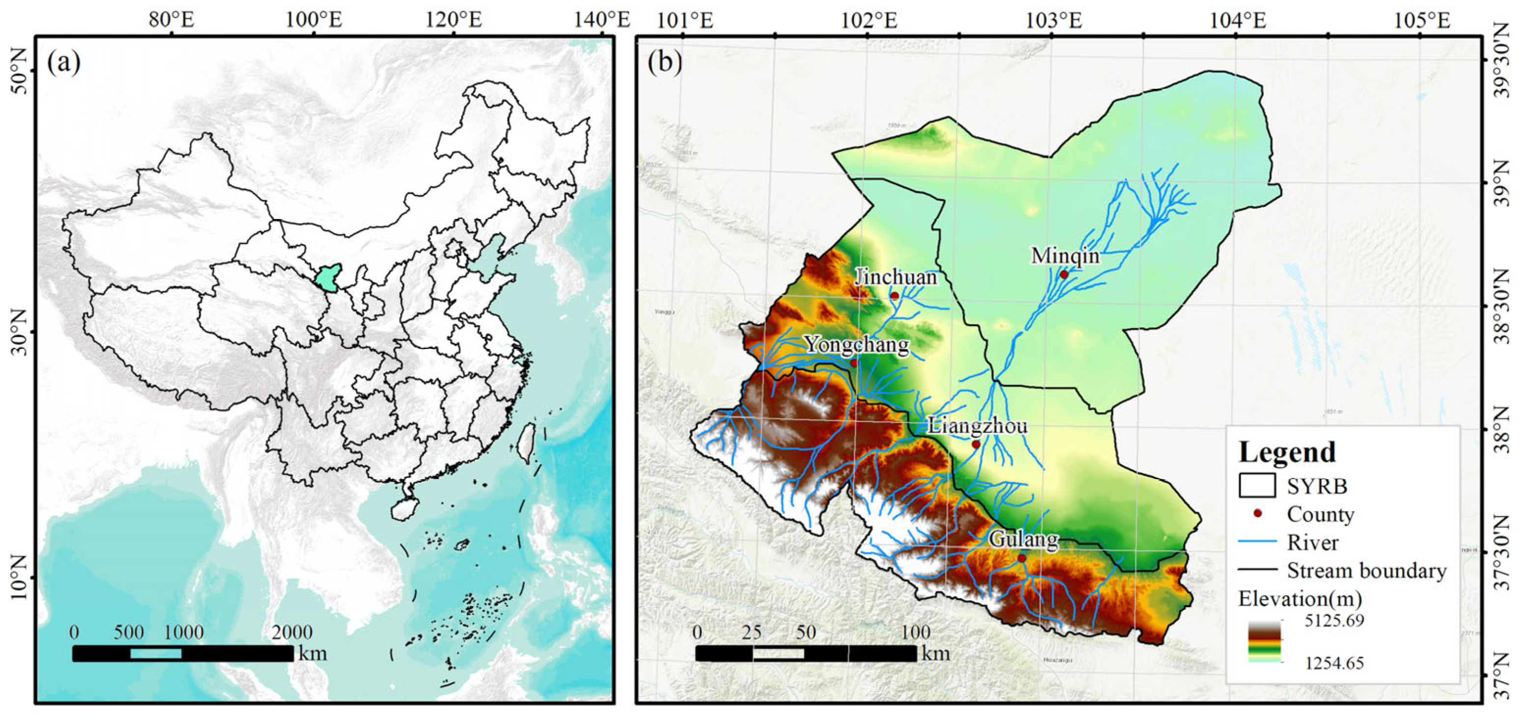
The Shiyang River Basin (SYRB) (101°41′ E–104°16′ E, 36°29′ N–39°27′ N) is a typical inland river basin in China’s arid northwest, covering approximately 41,600 km² in the Hexi Corridor of the Gansu Province. The Shiyang River originates in the Qilian Mountains and is mainly fed by precipitation, snowmelt, and glacial melt. The basin features a distinct mountain–oasis–desert ecosystem, with elevation decreasing from southwest to northeast [17] (Figure 1). The SYRB has a temperate continental arid climate, characterized by strong solar radiation and large diurnal temperature variations. The mean annual temperature is 7.75 °C, and the mean annual precipitation is 197.96 mm. This is far lower than the potential evaporation, which exceeds 1000 mm, indicating severe aridity [18]. Natural conditions and human activities vary greatly across the basin. The upstream Qilian Mountains serve as the main runoff generation and water conservation area. The midstream contains extensive urban and agricultural zones, where water resource exploitation and socioeconomic activities are most intensive. The downstream Minqin Basin, located between the Badain Jaran and the Tengger deserts, represents a typical terminal inland river ecosystem. This region is extremely fragile and sensitive to water availability, and has long suffered from groundwater overextraction, lake shrinkage, and desertification, resulting in severe ecological degradation.

2.2. Data Sources and Preprocessing

The multi-source data used in this study are summarized in

Table 1. Data sources.

Name	Resource	Resolution	Purpose
Landsat 5 TM	GEE a	30 m	Ecological quality
Landsat 7 ETM +		30 m
Landsat 8 OLI/TIRS		30 m
Population density (POP)	Resource and Environmental Science Data Platform b	1 km	Socioeconomic development
Gross domestic product (GDP)		1 km
Nighttime light (NTL)	National Tibetan Plateau/Third Pole Environment Data Center c	1 km
Precipitation (PRE)		1 km	Driving factor analysis
Temperature (TEM)		1 km
Evapotranspiration (EVP)		1 km
Elevation (DEM)		1 km
Land cover datasets (CLCD)	Zenodo d	30 m
Water use (WU)	Figshare Dataset e	10 km
Runoff (Q)	Early Warning Data Store f	5 km
Net Primary Productivity (NPP)	NASA-EARTHDATA g	500 m	gRSEI validation
Ecosystem Quality Index (EQI)	Global Change Research Data Publishing & Repository h	250 m

Notes: ^a https://developers.google.cn/earth-engine (accessed on 2 August 2025); ^b https://www.resdc.cn (accessed on 21 August 2025); ^c https://data.tpdc.ac.cn/home (accessed on 8 September 2025); ^d https://zenodo.org/ (accessed on 8 September 2025); ^e https://figshare.com/; ^f https://ewds.climate.copernicus.eu/ (accessed on 25 September 2025); ^g https://lpdaac.usgs.gov/products/mod17a3hgfv061/ (accessed on 29 January 2026); ^h https://geodoi.ac.cn (accessed on 11 May 2026).

. Remote sensing data were mainly derived from Landsat series imagery through the Google Earth Engine (GEE) platform. Considering the local vegetation growing season, only images from June to September of each year were selected. Standard preprocessing, including radiometric calibration, cloud masking, and gap filling, was conducted in GEE. Missing pixels caused by cloud cover or sensor differences were interpolated to ensure temporal continuity. Socioeconomic data included population density (POP), gross domestic product (GDP), and nighttime light (NTL), with NTL obtained from the PANDA dataset. Driving factors comprised natural environmental, land-use, and water-related variables. Natural factors included precipitation (PRE), temperature (TEM), evapotranspiration (EVP), and elevation (DEM). Land cover was derived from the annual China Land Cover Dataset (CLCD), and water-related factors included water use (WU) and runoff (Q). Net primary productivity (NPP) data were obtained from NASA EARTHDATA for gRSEI validation. To ensure spatial consistency, all datasets were processed in ArcGIS 10.8 and resampled to 1km resolution. Bilinear interpolation was applied to continuous variables, while nearest-neighbor interpolation was used for categorical data. All datasets were projected to Krasovsky_1940_Albers.

3. Methods

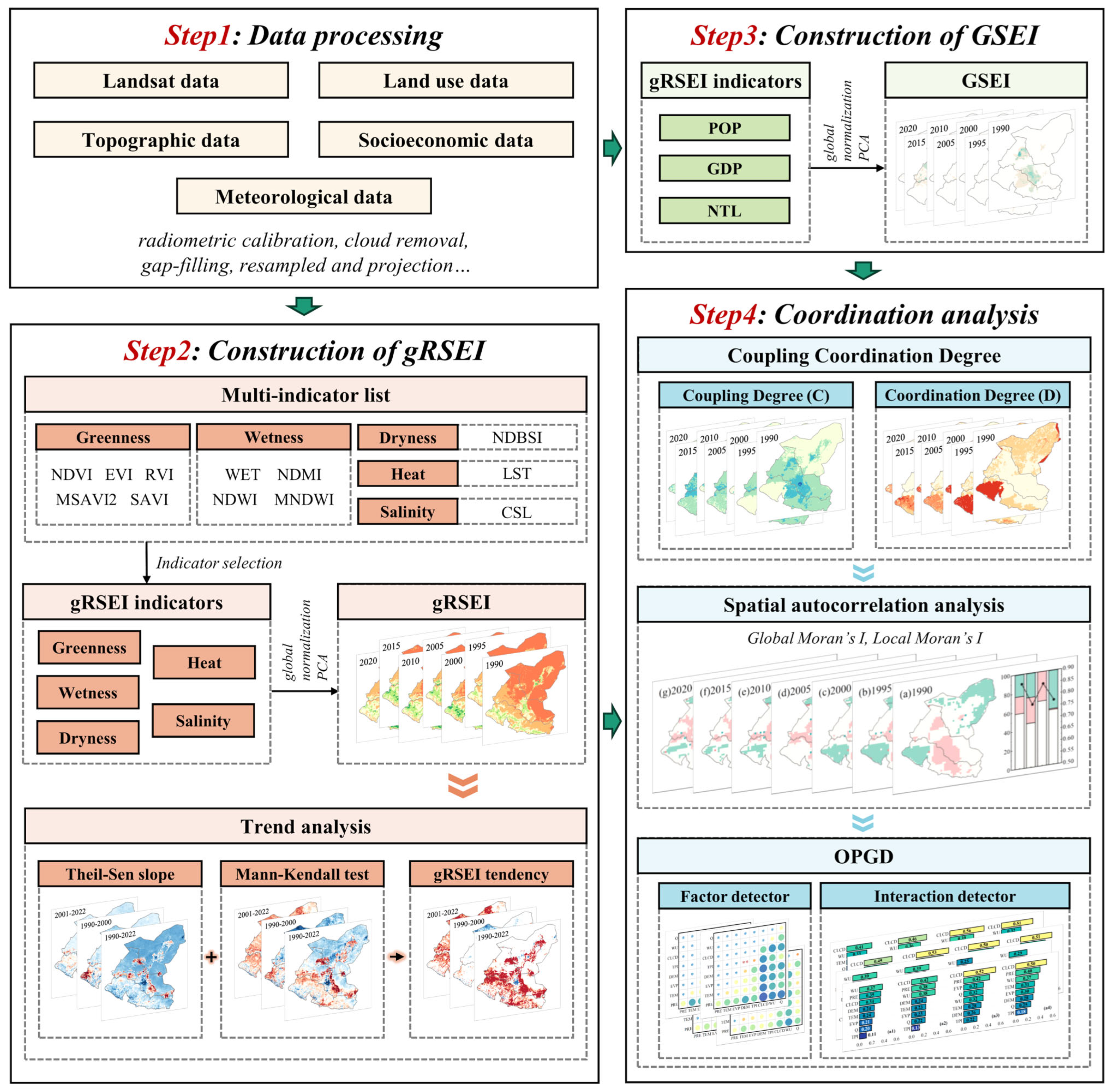
The methodology comprises four modules (Figure 2): (1) gRSEI and GSEI model construction, involving optimal indicator selection, global normalization, and PCA; (2) time-series trend analysis using the Theil–Sen median method and the Mann–Kendall test; (3) eco-socioeconomic relationship assessment through CCD; and (4) coordination analysis employing global/local Moran’s I for spatial autocorrelation and OPGD for driving factor analysis.

3.1. Original RSEI Model

RSEI [7] provides a comprehensive assessment of EQ through four key indicators: Greenness, which represents vegetation coverage and growth status, is quantified by NDVI. Wetness, which reflects surface and soil moisture conditions, is characterized by the wetness component of the Tasseled Cap transformation (WET). Dryness captures both natural bare soil and artificial impervious surfaces and is represented by NDBSI. Heat is expressed by Land Surface Temperature (LST), derived from the inversion of corrected brightness temperature. These indicators are normalized and integrated through PCA, with the first principal component (PC1) used to construct the final RSEI. The formulation is given by:

$$RSEI = f\left\{G,W,D,H\right\}$$

(1)

where G, W, D, and H are indicators of greenness, wetness, dryness, and heat, respectively.

3.2. gRSEI Model

3.2.1. Indicator Selection

To accurately capture local environmental characteristics, a multi-indicator list was established for gRSEI. For greenness indicators, the S/N ratio [19] was applied to assess their ability to mitigate soil background interference and extract valid vegetation information, thereby identifying the optimal indicator. Wetness indicators were selected based on their correlations with in situ soil moisture to ensure stronger physical relevance. As for dryness and heat, the original NDBSI and LST were retained due to their clear ecological significance and wide applicability. Furthermore, a salinity indicator was introduced to characterize soil salinization in the study area. Given the spatial heterogeneity of soil texture and geomorphology, which may constrain the applicability of single salinity indices, the Comprehensive Salinity Index (CSI) is adopted. This index combines three widely used salinity indicators, namely SI-T, NDSI, and SI3, to improve the robustness of salinization assessment. The complete indicator system is presented in

Table 2. Multi-indicator list.

Indicator		Calculation Formula	References
Greenness	NDVI	$NDVI=\left({\rho }_{NIR}-{\rho }_{RED}\right)/\left({\rho }_{NIR}+{\rho }_{RED}\right)$	[7]
	EVI	$EVI=G\left({\rho }_{NIR}-{\rho }_{RED}\right)/\left({\rho }_{NIR}+C_1{\rho }_{RED}-C_2{\rho }_{BLUE}+L\right)$	[20]
	RVI	$RVI={\rho }_{NIR}/{\rho }_{RED}$	[20]
	MSAVI2	$MSAVI2={\displaystyle \frac{1}{2}}\times \left(2\left({\rho }_{NIR}+1\right)-\sqrt{{\left(2{\rho }_{NIR}+1\right)}^2-8\left({\rho }_{NIR}-{\rho }_{RED}\right)}\right)$	[20]
	SAVI	$SAVI=\left(1+L\right)\times \left({\rho }_{NIR}-{\rho }_{RED}\right)/\left({\rho }_{NIR}+{\rho }_{RED}+1\right)$	[21]
Wetness	WET	$WET=a_1{\rho }_{BLUE}+a_2{\rho }_{GREEN}+a_3{\rho }_{RED}+a_4{\rho }_{NIR}-a_5{\rho }_{SWIR1}-a_6{\rho }_{SWIR2}$	[7]
	NDMI	$NDMI=\left({\rho }_{NIR}-{\rho }_{SWIR1}\right)/\left({\rho }_{NIR}+{\rho }_{SWIR1}\right)$	[20]
	NDWI	$NDWI=\left({\rho }_{GREEN}-{\rho }_{NIR}\right)/\left({\rho }_{GREEN}+{\rho }_{NIR}\right)$	[20]
	MNDWI	$MNDWI=\left({\rho }_{GREEN}-{\rho }_{SWIR1}\right)/\left({\rho }_{GREEN}+{\rho }_{SWIR1}\right)$	[20]
Dryness	NDBSI	$NDBSI=\left(IBI+SI\right)/2$ $IBI={\displaystyle \frac{2\frac{{\rho }_{SWIR1}}{{\rho }_{SWIR1}+{\rho }_{NIR}}-\left(\frac{{\rho }_{NIR}}{{\rho }_{NIR}+{\rho }_{RED}}+\frac{{\rho }_{GREEN}}{{\rho }_{GREEN}+{\rho }_{SWIR1}}\right)}{2\frac{{\rho }_{SWIR1}}{{\rho }_{SWIR1}+{\rho }_{NIR}}+\left(\frac{{\rho }_{NIR}}{{\rho }_{NIR}+{\rho }_{RED}}+\frac{{\rho }_{GREEN}}{{\rho }_{GREEN}+{\rho }_{SWIR1}}\right)}}$ $SI={\displaystyle \frac{\left({\rho }_{SWIR1}+{\rho }_{RED}\right)-\left({\rho }_{NIR}+{\rho }_{BLUE}\right)}{\left({\rho }_{SWIR1}+{\rho }_{RED}\right)+\left({\rho }_{NIR}+{\rho }_{BLUE}\right)}}$	[7]
Heat	LST	$LST={\displaystyle \frac{T}{\left(1+\left(\frac{\lambda T}{\rho }\right)\ln \epsilon \right)}}-273.15$	[7]
Salinity	CSI	$CSI=\left(SI-T+NDSI+SI3\right)/3$ $SI-T={\rho }_{RED}/{\rho }_{NIR}$ $NDSI=\left({\rho }_{RED}-{\rho }_{NIR}\right)/\left({\rho }_{RED}+{\rho }_{NIR}\right)$ $SI3=\sqrt{{{\rho }_{GREEN}}^2+{{\rho }_{RED}}^2}$	[22]

Note [11]: ρ_BLUE, ρ_GREEN, ρ_RED, ρ_NIR, ρ_SWIR1, ρ_SWIR2 represent the blue band, green band, red band, near-infrared band, shortwave infrared 1 band, and shortwave infrared 2 band in remote sensing images, respectively. G is the gain factor; C₁ and C₂ represent the atmospheric resistance factor for red and blue band, respectively; L stands for the canopy background adjustment factor; Empirical values were adopted for all parameters, with G = 2.5, C₁ = 6, C₂ = 7.5, and L = 1 in EVI calculation. L is the soil adjustment factor in SAVI calculation, with L = 0.5 for improved performance across most land cover conditions. T represents the temperature value at the sensor; λ is the thermal infrared band, ρ is a fixed variable of 1.438 × 10⁻² mΚ, and ε is the surface emissivity.

. The formula for the S/N ratio is given as follows:

$$S/N={\displaystyle \frac{\overline{VI}}{2\delta }}$$

(2)

where $\overline{VI}$ is the mean and δ is the standard deviation of the greenness indicator values under identical vegetation conditions.

3.2.2. gRSEI Calculation

To ensure interannual comparability, this study normalizes all indicators using extreme values from the entire study period, replacing the original annual normalization approach to prevent obscuring long-term trends. The formula is as follows:

$$X_{norm}={\displaystyle \frac{X-X_{gmin}}{X_{gmax}-X_{gmin}}}$$

(3)

where X_norm is the normalized indicator value, X is the original indicator value, and X_gmax and X_gmin represent the maximum and minimum values of the indicator over the entire study period, respectively.

PCA is conducted with two key improvements. A covariance matrix computed from the full study period dataset is used instead of annual covariance matrices to enhance temporal consistency. The gRSEI₀ calculation is adaptively determined based on PC1 loadings to ensure positive correlation with EQ. The formula is defined as:

$${gRSEI}_0=\left\{\begin{array}{c}PC1\left(G,W,D,H,S\right), loading\left(G,W\right)>0 \\ 1-PC1\left(G,W,D,H,S\right), loading\left(G,W\right)<0 \end{array}\right.$$

(4)

where G, W, D, H, and S are indicators of greenness, wetness, dryness, heat, and salinity, respectively; loading() means the loadings of indicators in PC1.

Finally, gRSEI₀ is normalized to the range [0, 1] to derive gRSEI, with values closer to 1 indicating better EQ.

3.3. GSEI Model

This study introduces the gRSEI framework into socioeconomic research to propose the GSEI. The index integrates POP, GDP, and NTL as core input variables, which represent population carrying capacity, economic output, and the intensity of human activities, respectively, thereby characterizing regional socioeconomic conditions from multiple dimensions. The integration of multi-source spatial data reduces structural bias of single proxy indicators and enhances the comprehensive representation of spatial socioeconomic heterogeneity. The construction of GSEI employs the aforementioned time-series normalization and PCA approach, and the model formulation is described as follows:

$$GSEI=f\left\{POP,GDP,NTL\right\}$$

(5)

3.4. Trend Analysis

The Theil–Sen (TS) slope (β) is calculated as the median of all pairwise slopes to quantify the long-term trend, with the formula [23] as follows:

$$\beta =Median\left\{{\displaystyle \frac{x_j-x_i}{j-i}}\right\};\forall j>i$$

(6)

where Median{ } is the median function; x_i and x_j denote the values of the time series at the time points i and j, respectively; and β represents the estimated median slope.

The Mann–Kendall (MK) test computes the standardized statistic Z_MK through a normalized test statistic derived from the difference between concordant and discordant pairs [24], computed as:

$$S={\displaystyle \sum _{i=1}^{n-1}}{\displaystyle \sum _{j=i+1}^n}sgn\left(x_j-x_i\right);i<j\le n$$

(7)

$$sgn\left(x_j-x_i\right)=\left\{\begin{array}{c}1,{ x}_j-x_i>0 \\ 0, { x}_j-x_i=0\\ -1,{ x}_j-x_i<0\end{array}\right.$$

(8)

$$Z_{MK}=\left\{\begin{array}{c}{\displaystyle \frac{s-1}{\sqrt{var\left(S\right)}}}; S>0\\ 0; S=0\\ {\displaystyle \frac{s+1}{\sqrt{var\left(S\right)}}}; S<0\end{array}\right.$$

(9)

where sgn(·) denotes the signum function; S is the MK rank statistic; var(S) constitutes the tie-adjusted variance estimate of the rank statistic; and Z_MK represents the standardized test statistic that follows N(0, 1) under the null hypothesis.

Table 3. Classification criteria for ecological quality trends based on TS slope (β) and MK test significance (Z_MK).

Classification Criteria	Ecological Quality Trend
$\beta >0.0005$ and $\left|Z_{MK}\right|\ge 2.58$	highly significant improvement
$\beta >0.0005$ and $1.96\le \left|Z_{MK}\right|<2.58$	significant improvement
$\beta >0.0005$ and $1.645\le \left|Z_{MK}\right|<1.96$	mild improvement
$\left|\beta \right|\le 0.0005$ or $\left|Z_{MK}\right|<1.645$	no significant change
$\beta <-0.0005$ and $1.645\le \left|Z_{MK}\right|<1.96$	mild degradation
$\beta <-0.0005$ and $1.96\le \left|Z_{MK}\right|<2.58$	significant degradation
$\beta <-0.0005$ and $\left|Z_{MK}\right|\ge 2.58$	highly significant degradation

details the comprehensive criteria for final trend interpretation by combining β and Z_MK [25].

3.5. Coupling Coordination Degree (CCD)

CCD quantifies the interaction and coordination between systems as a composite metric. The coupling degree (C) measures the intensity of interactions, while the coordination degree (D) assesses the quality of synergistic development. The formulas are as follows [26]:

$$C=2\sqrt{{\displaystyle \frac{U_1\times U_2}{{\left(U_1+U_2\right)}^2}}}$$

(10)

$$T=\alpha U_1+\beta U_2$$

(11)

$$D=\sqrt{C\times T}$$

(12)

where U₁ and U₂ denote the normalized evaluation scores of subsystems, scaled to [0, 1]; and T reflects the integrated development level, where equal weights (α = β = 0.5) emphasize the equivalent importance of both subsystems. The classification criteria are defined with reference to previous studies [27], as shown in

Table 4. Classification of CCD.

C Value Range	Coupling Stage	D Value Range	Coupling Coordination Degree
0 ≤ C ≤ 0.3	Low-level coupling	0 ≤ D ≤ 0.3	Low-level coordination
0.3 < C ≤ 0.5	Antagonistic stage	0.3 < D ≤ 0.5	Intermediate coordination
0.5 < C ≤ 0.8	Run-in stage	0.5 < D ≤ 0.8	Moderate coordination
0.8 < C ≤ 1	High-level coupling	0.8 < D ≤ 1	High-level coordination

.

3.6. Spatial Autocorrelation Analysis

Spatial autocorrelation quantifies how geographic attribute values correlate across neighboring locations [28]. Global spatial autocorrelation analysis using Global Moran’s I evaluates the overall spatial clustering trend of the observed variable across the study area. Local spatial autocorrelation analysis employing Local Moran’s I identifies statistically significant clustering patterns and their spatial distributions. The calculation formulas for both are as follows:

$$Global Mora{n}^{\prime }s I={\displaystyle \frac{n{\displaystyle {\sum }_{i=1}^n}{\displaystyle {\sum }_{j=1}^n}{W}_{ij}\left(x_i-\overline{x}\right)\left(x_j-\overline{x}\right)}{\left({\displaystyle {\sum }_{i=1}^n}{\displaystyle {\sum }_{j=1}^n}{W}_{ij}\right){\displaystyle {\sum }_{i=1}^n}{\left(x_i-\overline{x}\right)}^2}}$$

(13)

$$Local Mora{n}^{\prime }s I={\displaystyle \frac{n\left(x_i-\overline{x}\right){\displaystyle {\sum }_{j=1}^n}{W}_{ij}\left(x_j-\overline{x}\right)}{{\displaystyle {\sum }_{i=1}^n}{\left(x_i-\overline{x}\right)}^2}}$$

(14)

where n is the total number of spatial units within the study area; x_i and x_j represent the observed values at unit i and j, respectively; $\overline{x}$ corresponds to the mean value of all observed values; and W_ij constitutes the spatial weight matrix that quantifies the connection intensity between unit i and j.

3.7. Optimal Parameters-Based Geographical Detector (OPGD)

The Geographical Detector is a statistical method that identifies driving factors by analyzing relationships between geographical variables. To address its limitations in spatial scale and data discretization, the OPGD determines optimal discretization methods and the number of breaks by maximizing the q-statistic, thereby enhancing model robustness [29].

The factor detector module examines the explanatory power of independent variables (X) on the spatial heterogeneity of dependent variable (Y), with the formula as follows:

$$q=1-{\displaystyle \frac{{\displaystyle {\sum }_{h=1}^L}{N}_h{\sigma }_h^2}{N{\sigma }^2}}=1-{\displaystyle \frac{SSW}{SST}}$$

(15)

$$SSW={\displaystyle \sum _{h=1}^L}{N}_h{\sigma }_h^2$$

(16)

$$SST=N{\sigma }^2$$

(17)

where q represents the explanatory power of X for the spatial heterogeneity of Y; L donates the number of layers of the independent variables; N_h and N denote the sample sizes of layer h and the entire study region, respectively; ${\sigma }_h^2$ and σ² are the variances of layer h and the total region; SSW is the within-layer variance sum; and SST is the total variance.

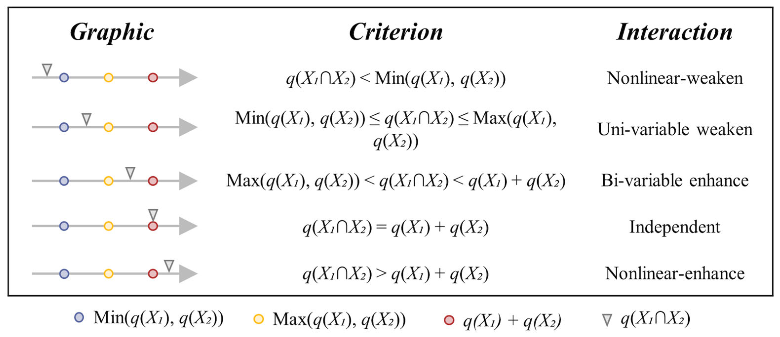
The interaction detector module analyzes how two independent variables (X₁ and X₂) jointly influence the spatial heterogeneity of dependent variable (Y). The interaction types are illustrated in Figure 3.

4. Results

4.1. gRSEI

In this study, gRSEI was constructed using the selected greenness and wetness indicators, combined with the dryness indicator (NDBSI), heat indicator (LST), and salinity indicator (CSI). EVI demonstrates the highest S/N ratio among the candidate greenness indicators (

Table 5. Multi-year average S/N ratios of greenness indicators.

Indicator	NDVI	EVI	RVI	MVASI	SAVI
S/N	1.1709	1.7254	0.6610	1.3070	1.2867

) and was therefore selected. NDMI exhibits the strongest correlation with in situ soil moisture measurements (

Table 6. Correlation coefficients (r) between wetness indicators and soil moisture.

Indicator	WET	NDMI	NDWI	MNDWI
r	0.670	0.674	−0.640	−0.526

). Its band combination of near-infrared (NIR) and shortwave infrared (SWIR) is sensitive to vegetation water content, making it the optimal wetness indicator.

4.1.1. Evaluation of gRSEI Performance

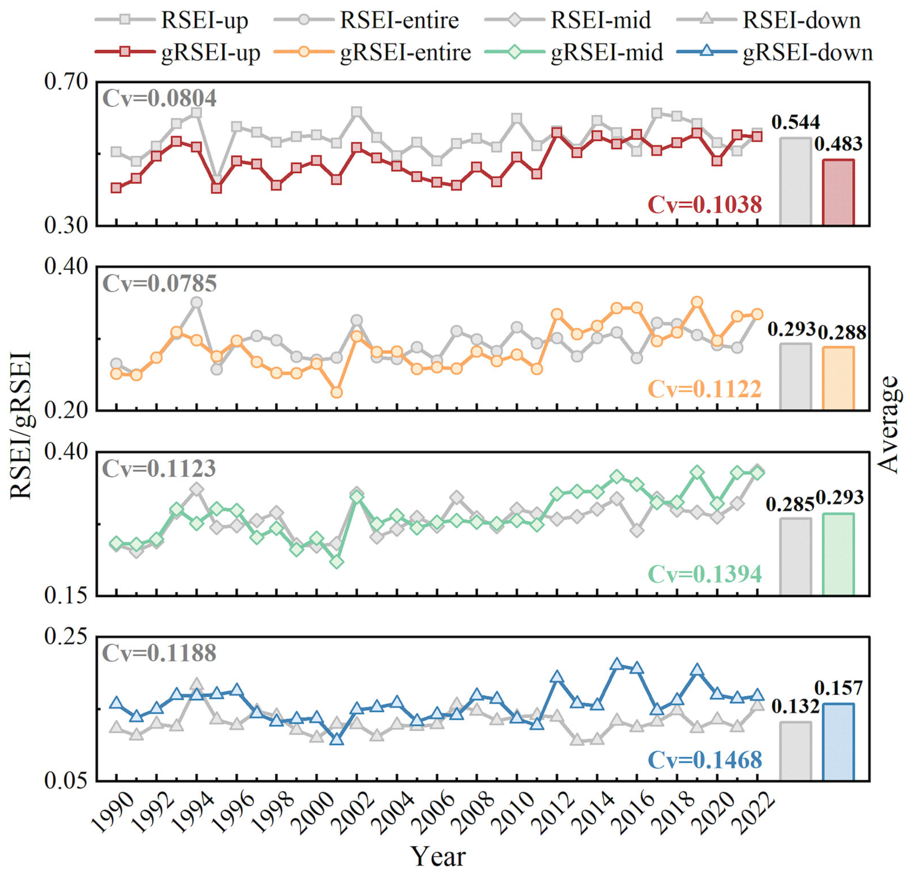
The performance of gRSEI was evaluated in terms of temporal stability and comprehensive capacity. Annual normalization in conventional RSEI facilitates within-year comparison but distorts interannual ecological baseline differences, overestimating EQ in UR while underestimating it in MR and DR (Figure 4). In contrast, gRSEI demonstrates higher interannual discriminability across the basin, with a basin-wide coefficient of variation (CV) of 0.1122, which is significantly higher than RSEI’s 0.0785.

By avoiding the overall variability inherent in annual normalization, gRSEI demonstrated a clear advantage in detecting ecological processes. It reveals stronger improvement trends in UR after the water transfer project (gRSEI slope: 0.0057 year⁻¹; RSEI slope: 0.0013 year⁻¹) and more distinct recovery turning points in DR. PCA results further confirm the integrative capability of gRSEI. The first principal component (PC1) of gRSEI shows a stable contribution rate of 86.58%, outperforming that of RSEI (mean 85.76%, minimum 78.92% in 1994). This indicates that gRSEI extracts more concentrated ecological information while maintaining temporal stability. Among PC1 loadings, the salinity index exhibits the largest absolute loading (−0.5074), validating its critical role in arid region ecological assessment and the effectiveness of the model improvement.

4.1.2. Spatiotemporal Variations of EQ

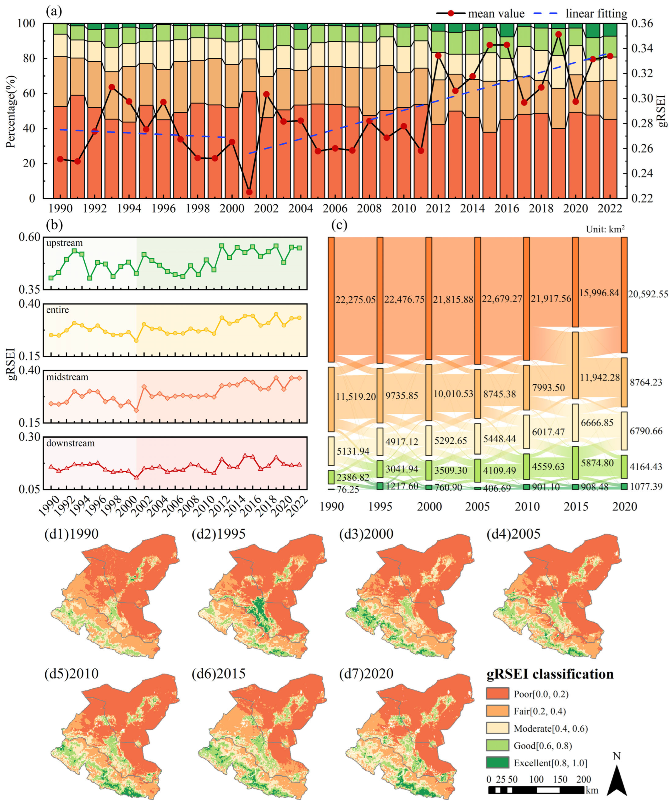
The gRSEI was applied to quantify the EQ in SYRB before and after the water transfer project, with values classified into five grades at 0.2 intervals (Figure 5). From the temporal perspective (Figure 5a), the basin-wide mean gRSEI increased during 1990–1993, then fluctuated downward to a minimum of 0.2252 in 2001. It briefly peaked at 0.3035 in 2002, remained around 0.27 during 2003–2011, then increased steadily after 2012, reaching 0.3339 in 2022. In terms of grade proportions (Figure 5c), poor and fair levels dominated the basin, maintaining over 75% of the total area before the water transfer. After project implementation, the proportion of moderate and higher classes gradually increased from 20.24% in 2001 to 32.52% in 2022, indicating overall improvement of EQ. Regionally (Figure 5b), UR exhibited the highest gRSEI values, with a multi-year average of 0.4834. It exhibited a fluctuating upward trend throughout the study period, with a faster increase observed after the water transfer. The MR and DR followed a similar trend to the basin-wide pattern. DR consistently maintained the lowest gRSEI throughout the entire study period, with a multi-year average of 0.1572, indicating relatively poor EQ. Spatially (Figure 5d), mountainous and valley areas in UR, together with oasis regions in MR, were persistently characterized by moderate or higher levels. In contrast, most of the DR remained classified as poor, except for limited oasis areas, forming the primary concentration of low EQ within the basin. After the project, good and excellent classes expanded in river valleys and oasis areas. However, arid regions surrounding oasis in DR remained dominated by poor levels, with only minor changes.

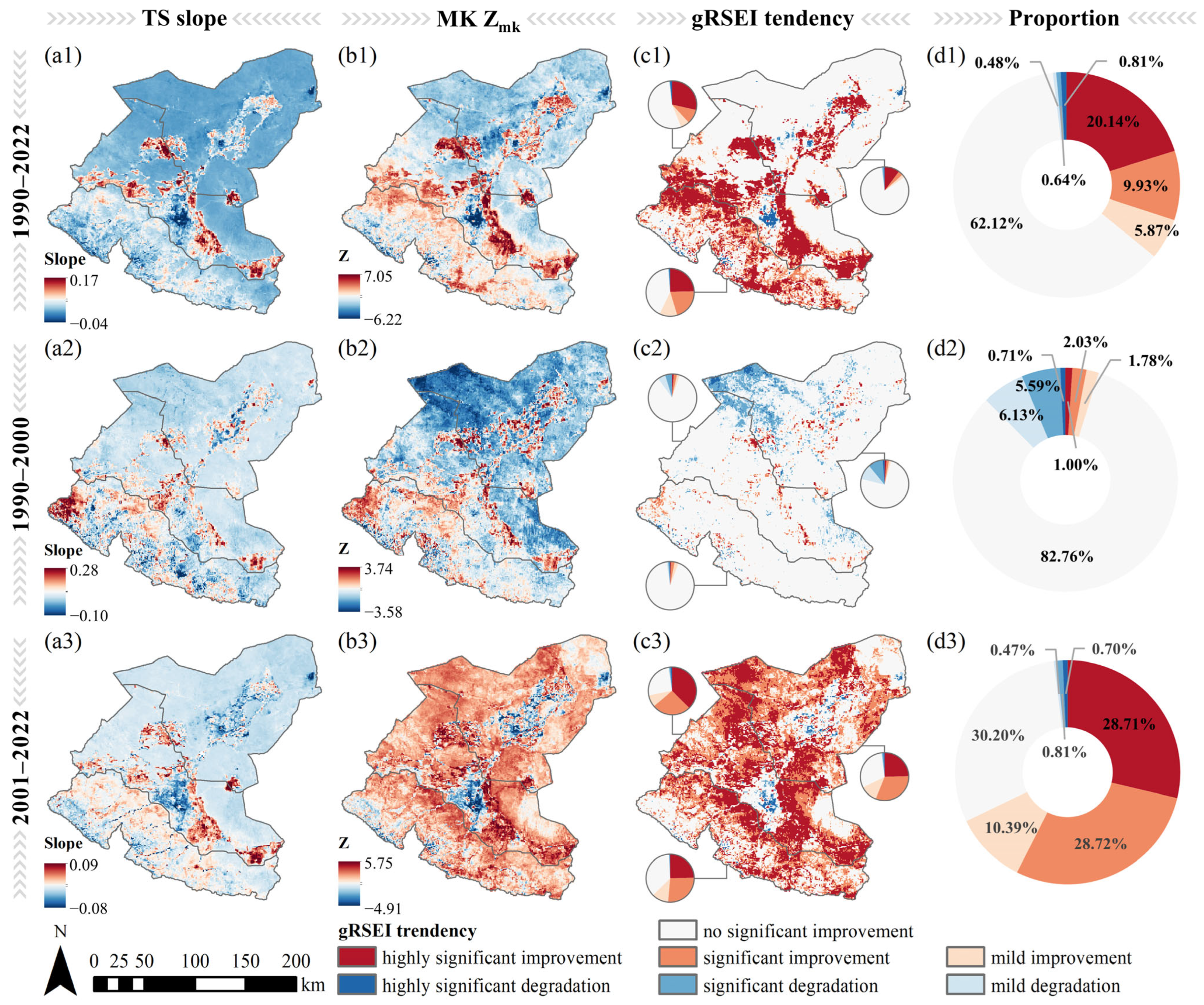
The gRSEI trend analysis (Figure 6) further reveals that EQ remained stable or improved across most of the SYRB during the study period, with degradation limited to only 1.93%. Improved areas were mainly located in the mountainous and valley areas of UR and in oasis areas of MR and DR, whereas degraded areas were mainly found within the core sections of the oasis in MR and DR. Before the water transfer project, stable and mildly degraded areas dominated, and 82.76% of the area showed no significant improvement. Degraded areas accounted for 12.43%, mainly concentrated in the western DR, whereas improved areas were limited and scattered. Following the project, the gRSEI trend changed markedly, and the proportion of improved areas increased to 67.82%, while degraded areas declined to 1.98%. Highly significant improvement occurred mainly within and along the edges of oasis, while degraded areas persisted in scattered patches inside some oasis regions. Regionally, UR showed the least ecological change prior to the project, while it had the largest proportion of degraded area, reaching 21.00%. After the project, the proportion of improved area increased to 71.92% in MR, the highest among the three subregions, compared to 67.75% in DR and 62.60% in UR. Overall, the post-project period saw a transition from predominantly stable or degraded conditions to predominant improvement across SYRB, with notable differences among subregions.

4.2. GSEI

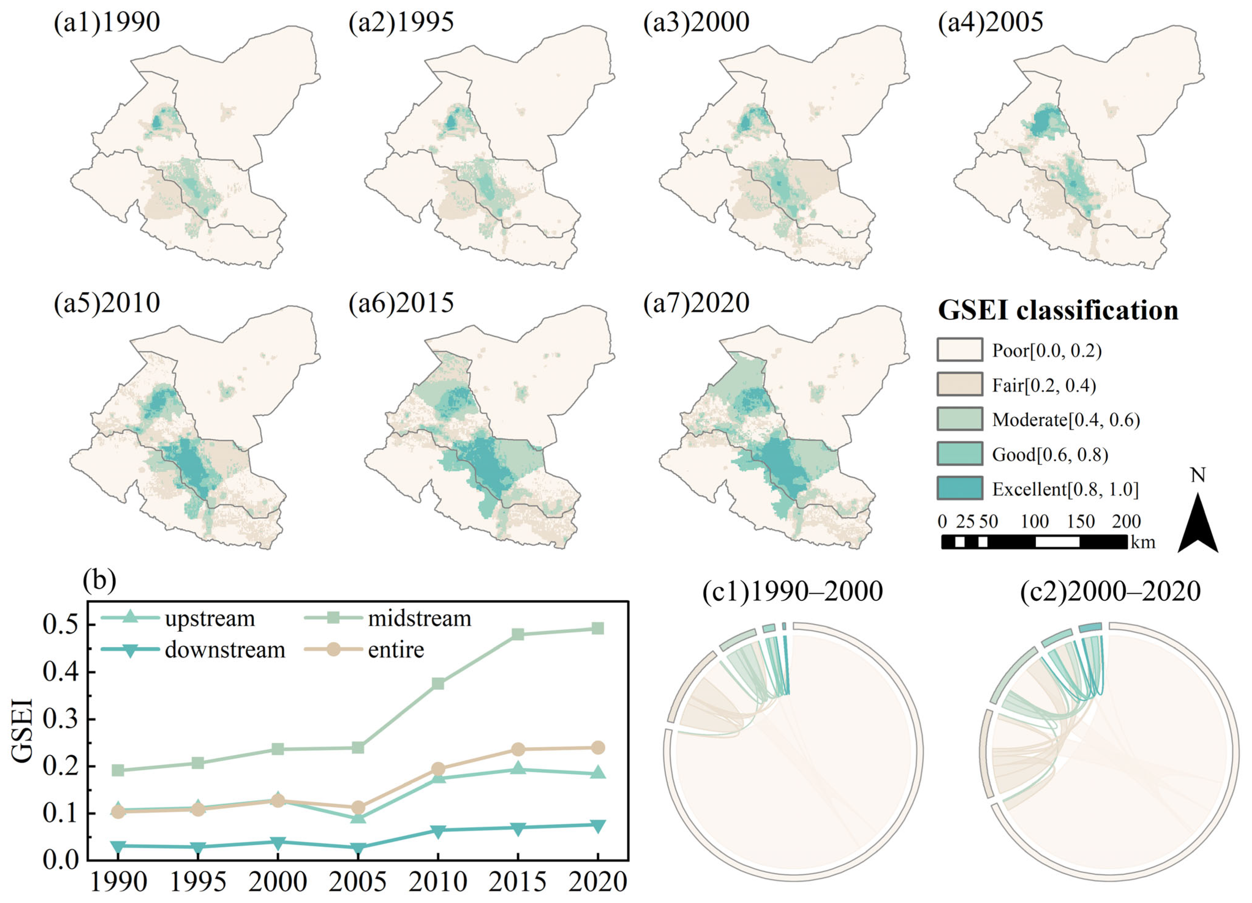
Figure 7 shows the spatiotemporal distribution of GSEI grades, reflecting the evolution of socioeconomic conditions before and after the water transfer project. Temporally (Figure 7b,c), socioeconomic development in SYRB entered an accelerated phase after the 2001 water transfer project. Before 2001, the basin-wide mean GSEI increased slowly and remained at around 0.1, with few grades changed. Specifically, 88.15% of the area remained stable, of which 78.42% remained in the poor category, while only 10.31% experienced grade upgrading. After the project, the mean GSEI exhibited a sustained upward trend, rising from 0.1132 in 2005 to 0.2403 in 2020, and areas experiencing grade improvement increased to 30.16%. Regionally, MR showed the highest socioeconomic development, followed by the UR, whereas DR maintained the lowest GSEI. Temporal trends in all subregions followed the basin-wide pattern, with minor fluctuations before the project and sustained growth thereafter. The MR exhibited the highest growth rate at 0.0169 year⁻¹. Spatially (Figure 7a), socioeconomic development in SYRB exhibited a pattern of core concentration with outward expansion. Before the project, poor and fair classes accounted for over 90% of the total area, with moderate and higher classes only sporadically distributed in parts of the MR oasis. During the post-project stage, high-value areas in the MR oasis expanded continuously. By 2020, MR formed a contiguous zone of good and excellent centered on Liangzhou, extending into parts of UR. In the DR oasis core, patches of moderate and higher grades were also present, while high-altitude areas of the UR and most of the DR remained dominated by poor class.

4.3. Ecological–Socioeconomic Coupling Coordination

4.3.1. Spatiotemporal Distribution of CCD

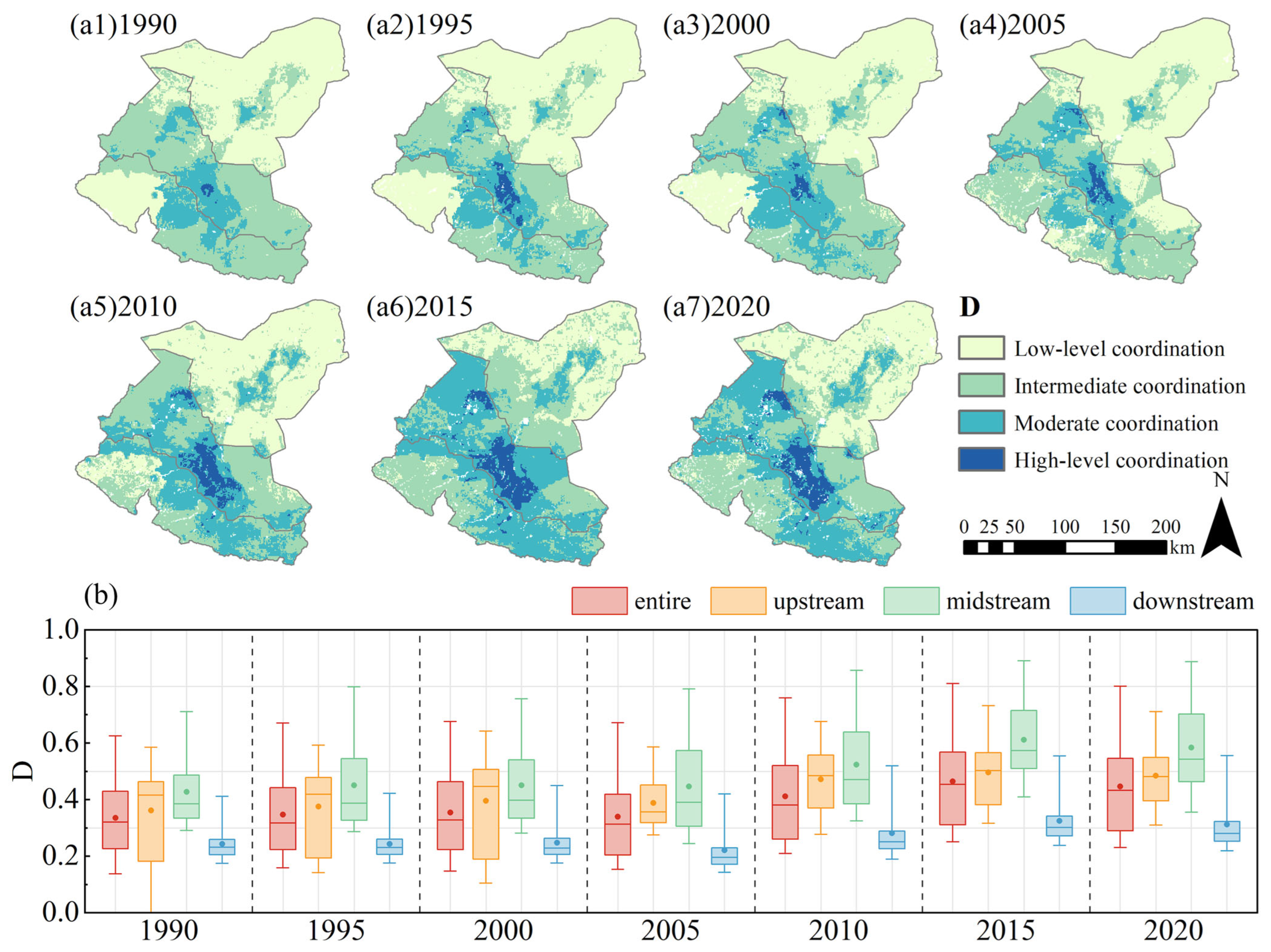
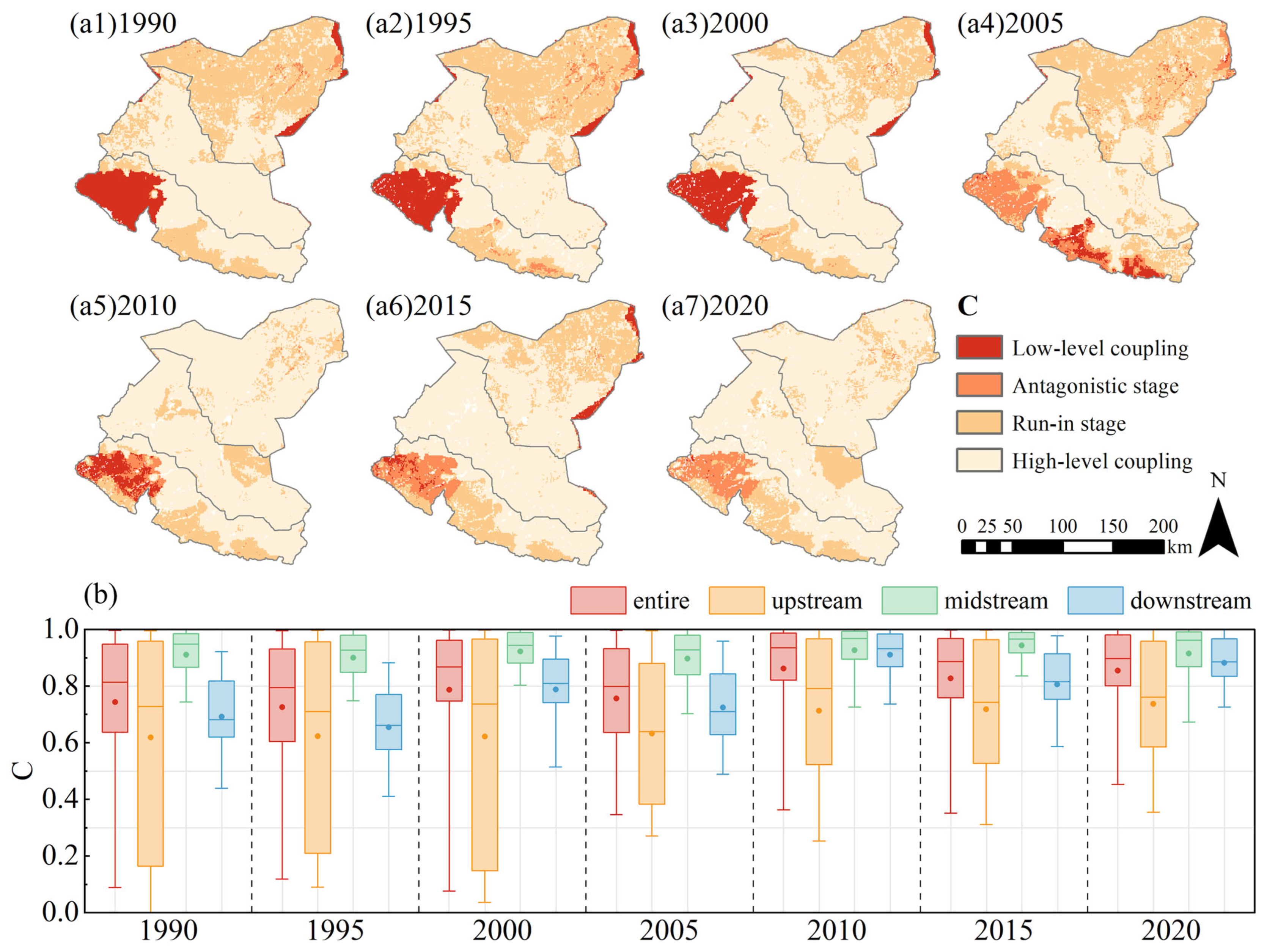
Spatial visualization and statistical analysis (Figure 8 and Figure 9) reveal the spatiotemporal heterogeneity of the CCD between the ecological and socioeconomic systems in SYRB. From 1990 to 2020, the basin-wide C and D increased from 0.7435 and 0.3359 to 0.8548 and 0.4465, respectively. The system progressed from the run-in stage toward high-level coupling while maintaining an intermediate coordination level, with pronounced spatial divergence.

The UR remained in the run-in stage, exhibiting the lowest mean C (0.6668) and substantial internal disparity, with its southwestern part predominantly characterized by low-level coupling or an antagonistic stage. Following the water transfer project, its D increased from 0.3961 to 0.4846. In contrast, the MR consistently maintained high-level coupling (mean 0.9169), and its D significantly improved from intermediate coordination (0.4280) to moderate coordination (0.5845), indicating enhanced interaction between the systems. While the DR maintained a relatively high mean C after 2010, it primarily reflected antagonistic interactions. Its D increased only from 0.2439 to 0.3121. This pattern of high-level coupling but low-level coordination made the DR the primary constraint on coordinated development across the SYRB.

4.3.2. Spatial Autocorrelation of D

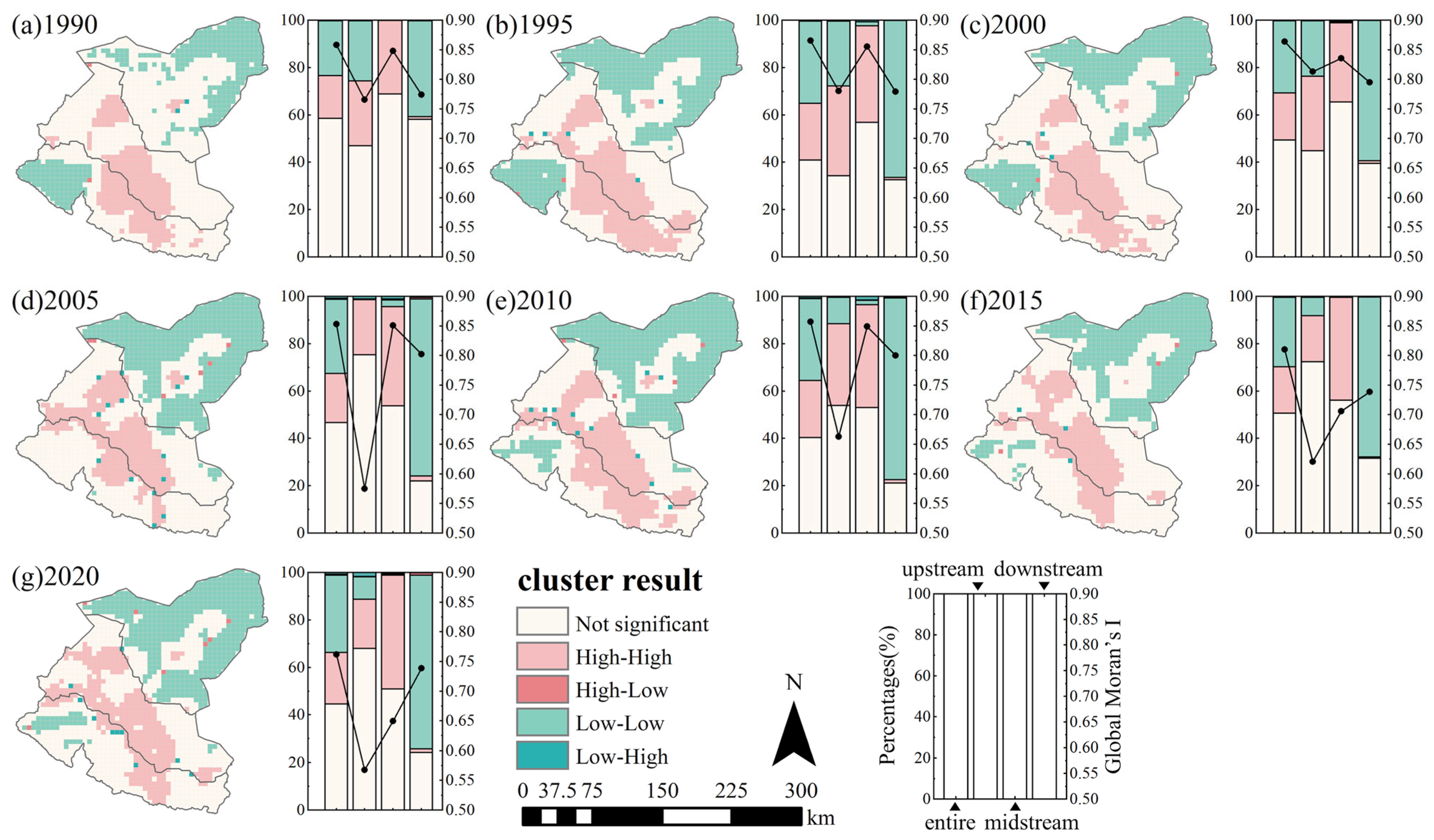
Global Moran’s I remained above 0.7 in all years (Figure 10), indicating persistent and significant spatial clustering of D. However, clustering intensity demonstrated a fluctuating downward trend over time. The index declined from 0.8585 in 1990 to 0.7616 in 2020, indicating a gradual shift toward a more balanced spatial pattern. Regionally, the UR exhibited the lowest and most volatile clustering, with its index dropping from 0.8130 in 2000 to 0.5679 in 2020, reflecting high spatial instability. In contrast, the DR displayed the most stable spatial pattern, with index values fluctuating narrowly between 0.73 and 0.80. The MR maintained the highest clustering intensity before 2010, stabilizing around 0.84, then declining to 0.6493 by 2020, also showing a clear downward trend.

Local Moran’s I analysis further revealed spatial heterogeneity. The MR was persistently dominated by expanding High–High (H–H) clusters, whose proportion grew from 31.03% to 47.88%, forming a stable high-level coordinated development cluster. Conversely, DR was overwhelmingly characterized by Low–Low (L–L) clusters, with its proportion increasing from 40.42% in 1990 to 73.1% in 2020, consistently maintaining an extensive and intense low-level coordinated development cluster. UR underwent the most complex transition. Prior to the water transfer project, H–H clustering increased from 27.39% to 31.44%, while L–L clusters decreased from 25.39% to 23.46%. Subsequently, these proportions declined to 20.84% and 9.37%, respectively. Concurrently, non-significant areas increased from 44.87% in 2000 to 67.92% in 2020, peaking at 72.40% in 2015. These shifts indicate substantial changes in the original clustering pattern of the UR, accompanied by increased spatial heterogeneity.

4.4. Driving Factor Analysis

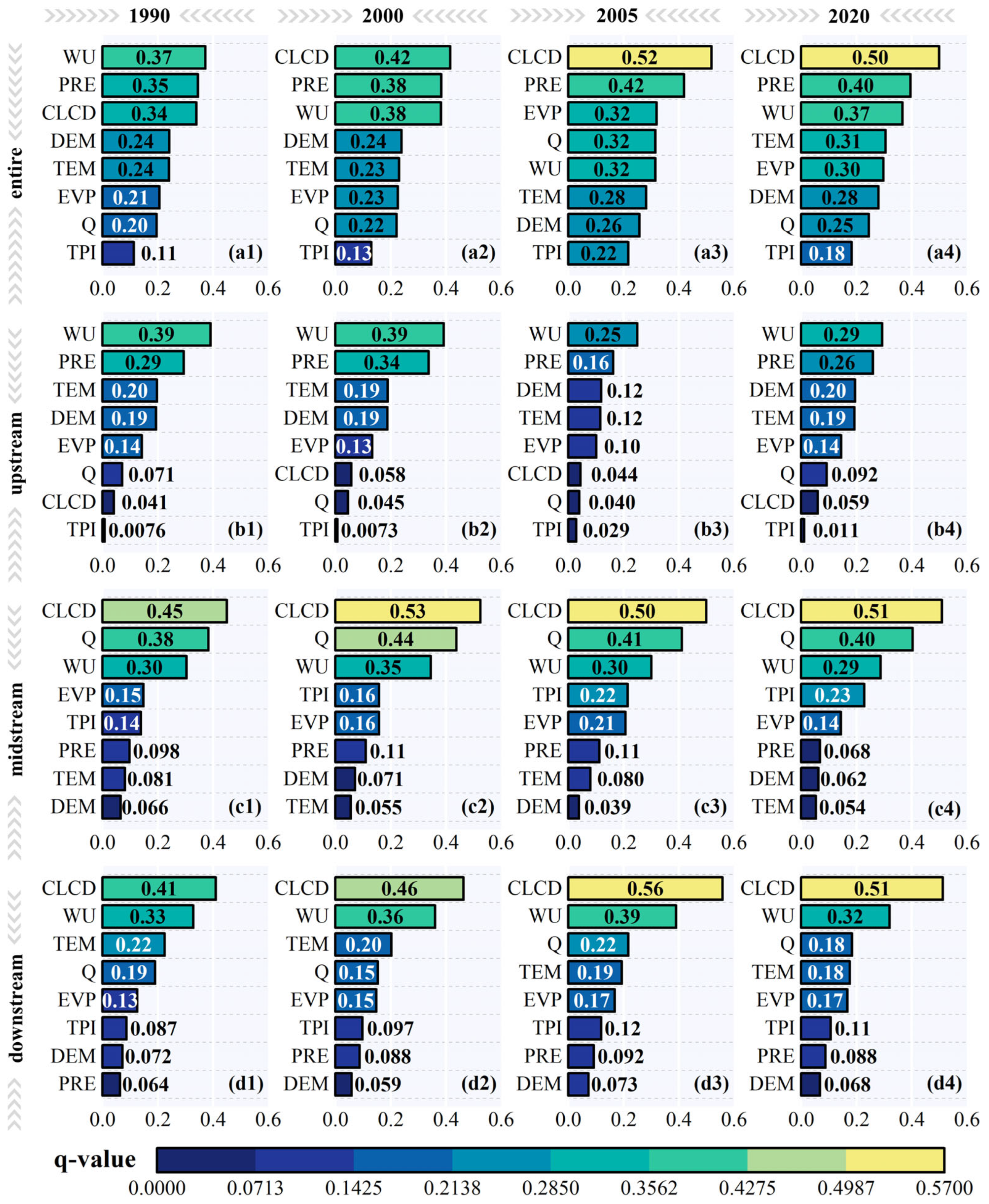
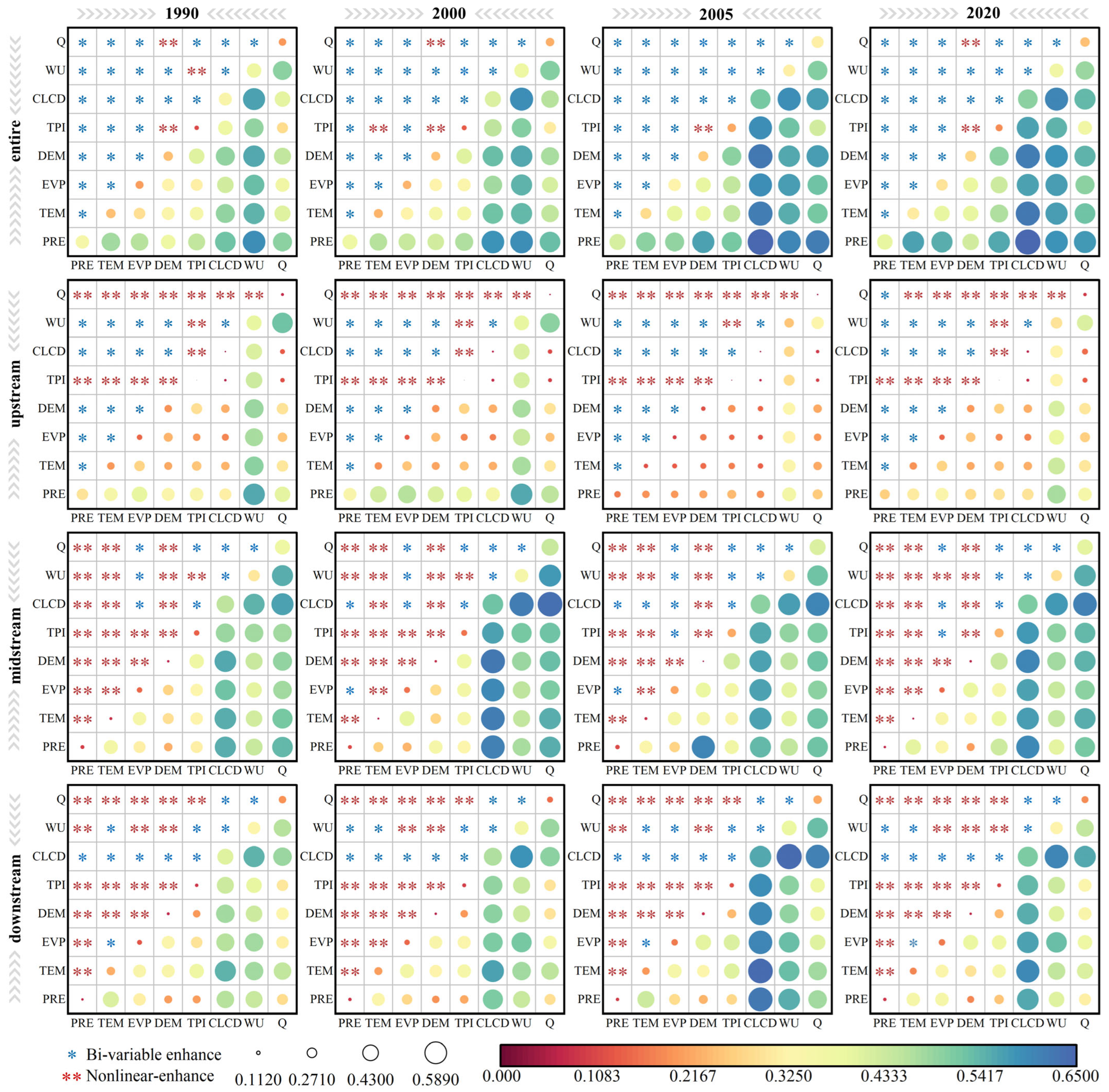
This study employed OPGD to analyze the key driving factors of eco-socioeconomic coordination degree in SYRB, revealing the temporal dynamics of both independent effects (Figure 11) and interaction effects (Figure 12). The q-value between any two factors showed either bi-variable or nonlinear enhancement, suggesting D was driven by a complex synergistic network rather than any single factor. At the basin scale, CLCD was the core driving factor. After the 2001 water transfer project, CLCD replaced WU as the persistently dominant factor. Its q-value rose from 0.3396 in 1990 to 0.4994 in 2020, while WU’s q-value declined from 0.3724 to 0.3668. Nevertheless, CLCD, WU, and PRE consistently ranked among the three leading factors throughout the study period, and their interactions formed a strong network. Before the transfer, the PRE-WU interaction dominated, with a combined q-value stable around 0.58. Subsequently, the PRE-CLCD interaction continuously strengthened, with q-values fluctuating above 0.64. TPI showed the lowest q-values across all years. Notably, although the independent q-value of Q was below 0.25 in most years, its interactions with other factors were significant, with the average q-value increasing from above 0.4 pre-diversion to over 0.5 post-diversion.

Spatially, the UR was dominated by WU and PRE. The q-values of CLCD, Q, and TPI remained below 0.1 over the long term, while other natural factors like TEM, DEM, and EVP fluctuated between 0.1 and 0.2. Except for generally lower explanatory power across all factors and their interactions in 2005, q-values in the UR showed no significant variation. In contrast, CLCD was the core factor in both MR and DR, with its q-value rising from 0.4509 and 0.4100 in 1990 to 0.5087 and 0.5129 in 2020, respectively. Water-related factors (WU and Q) exceeded natural factors in q-value, ranking second only to CLCD. The q-value of Q in MR was highest among the three subregions, averaging 0.4220 and peaking at 0.4925 in 2010. Notably, the q-value of Q was slightly higher than that of WU in MR, whereas the opposite pattern was observed in the DR. The differing dynamics of water–land synergy reflect spatial variation in the impacts of the water transfer project across the basin. CLCD-Q dominated in DR, with q-values above 0.6 since 1995, while CLCD-WU dominated in MR, increasing from 0.5479 in 1990 to 0.6042 in 2020 after the water transfer.

5. Discussion

5.1. Robustness and Validation of gRSEI

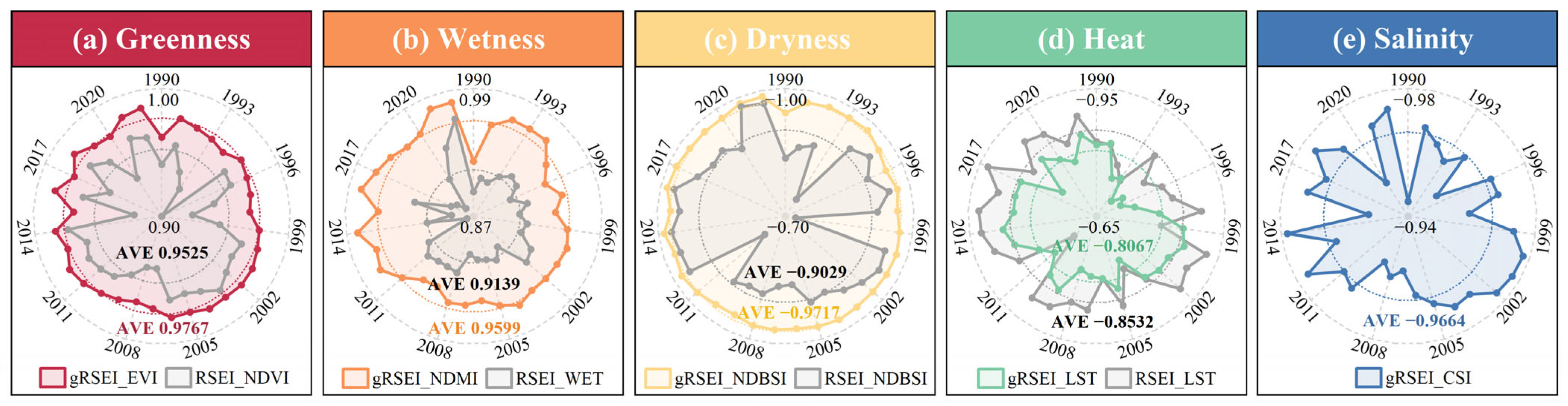
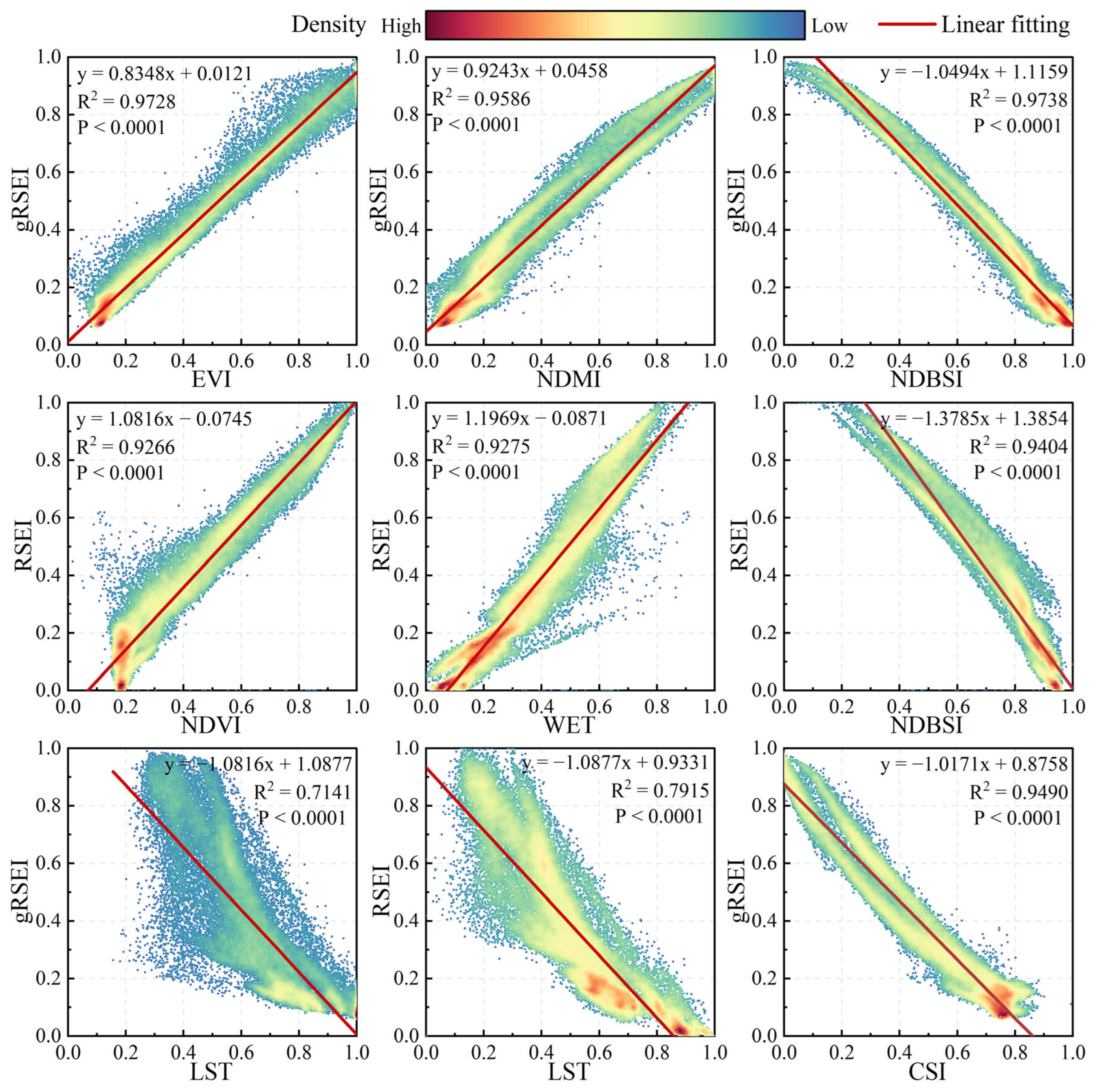
To further verify the robustness of gRSEI, pixel-scale correlation analyses between gRSEI/RSEI and each indicator were conducted annually (Figure 13 and Figure 14). Results indicate that greenness and wetness are positively correlated with both indices, whereas dryness, heat, and salinity are negatively correlated. All factors showed absolute annual correlations above 0.6, confirming both indices effectively represent key ecological elements with clear interpretability. The multi-year average correlations between gRSEI/RSEI and all indicators, except heat, exceeded 0.9 in absolute value, indicating strong agreement between the model outputs and core ecological variables such as vegetation, moisture, and salinity. The weaker correlation with heat is consistent with previous studies using modified remote sensing ecological indices, such as the MRSEI application in Dulan, Qinghai Province [30]. Pixel-scale scatter density plots (Figure 14) further indicate that the heat indicator (LST) shows more dispersed distributions along the fitted lines than other factors, suggesting greater uncertainty in its relationship with integrated EQ. This pattern arises from the indirect linkage between LST and EQ, as LST represents complex thermal processes controlled by surface energy balance and land surface conditions, and potential striping noise in Landsat LST retrievals [22]. By applying a more balanced weighting scheme in PCA, gRSEI weakens the dominance of heat while preserving its ecological significance, thereby emphasizing indicators more critical to SYRB. Consequently, compared to RSEI (Figure 13d), gRSEI shows stronger correlations with greenness, wetness, and dryness, and a weaker correlation with heat, enhancing its stability and ecological interpretability in long-term analysis.

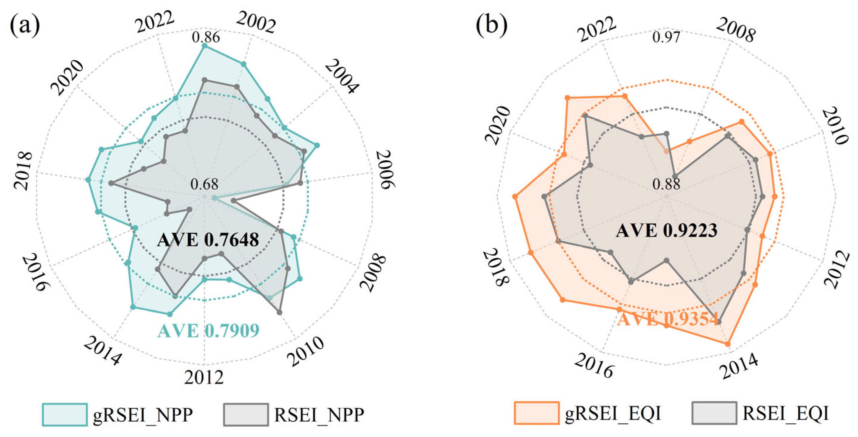
To evaluate the ability of gRSEI to represent EQ, Net Primary Productivity (NPP) and Ecosystem Quality Index (EQI) were introduced as independent ecological references. NPP, defined as the amount of dry matter fixed by vegetation through photosynthesis, is a widely used indicator of ecosystem productivity and functional status and thus serves as an effective reference for validating remote sensing ecological indices [31]. EQI was calculated using fractional vegetation cover (FVC), leaf area index (LAI), and gross primary productivity (GPP) as core indicators. Therefore, it reflects ecosystem structural integrity and functional stability and provides an independent reference for EQ assessment. Both gRSEI and RSEI show significant positive correlations with NPP and EQI (Figure 15). Except for 2006, 2007, and 2010, gRSEI exhibited higher correlations with NPP than RSEI. For EQI, gRSEI also showed stronger correlations than RSEI in most years, except 2007. These results indicate that gRSEI provides a more stable and consistent representation of EQ across space and time.

5.2. Spatiotemporal Eco-Socioeconomic Responses to the Water Transfer Project

The water transfer project not only increased water availability in SYRB, but also acted as an important hydrological intervention through water resource reallocation. The increased and more stable surface-water supply reduced groundwater dependence, promoted groundwater recovery, improved soil moisture, and replenished terminal lakes [32]. These changes supported oasis expansion and vegetation evapotranspiration. Consequently, the basin-wide gRSEI increased with the expansion of moderate-to-excellent EQ areas. Similar ecological benefits of water diversion have been reported in the Tarim River basin [33]. Improved water conditions further propagated to the socioeconomic system. Specifically, increased water availability and supply stability supported agricultural modernization, infrastructure development, and urban expansion [34], thereby driving a steady increase in GSEI. As both subsystems improved simultaneously, eco-socioeconomic coordination was strengthened, although clear spatial heterogeneity remained due to differences in water accessibility, ecological conditions, and human activity intensity.

The UR had a strong ecological baseline and consistently maintained the highest gRSEI, supported by forest conservation and strict mineral-exploitation restrictions [35]. However, its role as an ecological conservation and water-source area limited socioeconomic development. This constrained the conversion of ecological advantages into coordinated eco-socioeconomic development, especially in the southwestern UR, where high ecological quality coexisted with low socioeconomic development. Similar protection-driven constraints on UR development have also been observed in inland river basins such as the Heihe River Basin [36].

As the main agricultural and urban center, the MR has long faced competition among domestic, agricultural, and ecological water uses. After the implementation of the water transfer project, additional water supply stabilized irrigation and reduced pressure from competing water demands. This promoted agricultural development, vegetation recovery, and oasis expansion, making MR the region with the most significant EQ improvement (Figure 6). Meanwhile, the agricultural base, infrastructure, and locational advantages of MR enabled the rapid conversion of improved water availability into socioeconomic development. Therefore, high-GSEI areas expanded continuously and formed a contiguous zone centered on Liangzhou (Figure 7). This is consistent with previous findings linking eco-socioeconomic coordination to urban development [37]. A reinforcing positive feedback loop formed between EQ improvement and socioeconomic development, thereby improving coordination and expanding H–H clusters. Overall, MR can be regarded as the primary beneficiary of the water transfer project.

Although DR also benefited from the project, its ecological and socioeconomic responses remained limited. Ecological water replenishment alleviated drought stress, supported terminal-lake expansion, promoted groundwater recovery, and stabilized vegetation patches in the oasis–desert transition zone, thereby constraining desertification [38]. However, as the basin’s terminal region, DR is highly sensitive to upstream water allocation, evaporation loss, and groundwater conditions. Its EQ improvement was constrained by a fragile ecological baseline, historical desertification, and persistent soil salinization. In particular, potential secondary salinization risk persists in terminal wetlands characterized by shallow groundwater, strong evaporation, and limited natural salt drainage [39]. These constraints made EQ improvement more localized than in MR. On the socioeconomic side, improved water supply supported GSEI growth but did not substantially enhance development efficiency, as returns on water input remained low in ecologically fragile and industrially underdeveloped areas [40]. The high C value indicates close eco-socioeconomic dependence under limited water resources, while the low D value indicates this linkage did not translate into high-quality coordination. Although L–L clusters remained dominant, the declining Global Moran’s I indicates a gradual weakening of historical overexploitation-driven patterns. This indicates that the project played a structural and restorative role rather than directly improving coordination. Therefore, substantial coordination improvement requires sustained water supply, improved water management institutions, higher allocation efficiency, and technological interventions [41].

5.3. Driving Mechanisms of Eco-Socioeconomic Coordination

Previous studies in the Dagu and Yangtze River basins have commonly identified land use as a key driver of coordination [42,43]. In this study, CLCD replaced WU as the leading independent factor under the water transfer context and showed strong interactions with PRE and WU (Figure 11 and Figure 12). This indicates that coordination was jointly shaped by climate variability, land-use structure, and water-resource utilization, extending previous studies. After the project, external water supply and supporting governance jointly eased long-standing water constraints. Meanwhile, Q showed stronger explanatory power through interactions with other factors, indicating that water availability influenced coordination, mainly through its interactions with factors such as land use and precipitation. Although policy factors were not directly included in the OPGD model, their effects may have been reflected in changes in land-use structure, water-use intensity, and socioeconomic development patterns.

At the subregional scale, coordination in UR was primarily driven by WU and PRE, while CLCD contributed marginally. This was consistent with the ecological conservation role of UR and limited project impact. In contrast, MR and DR represented typical water–land synergistic systems, where CLCD acted as the core driver, followed by water-related factors. However, varying water constraints further shaped different coordination pathways. As a runoff corridor, MR was more directly constrained by water availability, with Q showing stronger explanatory power and pronounced interaction with CLCD, highlighting the combined effects of land development and stable water supply. In DR, however, limited water supply due to its location and diversion pattern intensified water-use competition. This made WU the dominant driver and the CLCD-WU interaction a prevailing driver, indicating that coordination improvement relied more on the coupled optimization of land use and water-use structure. Similar patterns have been observed in other arid water transfer basins, confirming that while diversion supports ecological restoration, sustainable development requires integrated water–land management [44].

The above insights guide differentiated basin management strategies. For UR, management should continue to prioritize water-source conservation, forest protection, and strict control of intensive development activities. For MR, governance should focus on regulating agricultural expansion, improving irrigation efficiency, and controlling water-intensive industries and land-development intensity. For DR, priority should be given to improving water-allocation efficiency, optimizing the water-use structure, and strengthening ecological restoration in terminal oasis and wetland areas.

5.4. Limitations and Future Improvements

Despite advances in long-term analysis, multi-indicator integration, and ecological– socioeconomic coordination assessment, several limitations remain.

First, the construction of both gRSEI and GSEI is constrained by data availability. For gRSEI, cloud cover and sensor differences may introduce noise or data gaps in certain years, potentially affecting accuracy despite interpolation. For GSEI, limited availability of long-term, gridded socioeconomic data remains a challenge. Advances in multi-source remote sensing data fusion and high-resolution socioeconomic datasets may further enhance the stability and explanatory power of both indices, thereby deepening the understanding of eco-socioeconomic relationships. In addition, the validation of gRSEI was mainly based on remote-sensing-derived variables. Although these datasets are useful for long-term and spatially continuous assessment, field-based ecological observations were limited in this study. Future work should integrate these observations to further validate the proposed framework and reduce uncertainty in ecological interpretation.

Second, although the CCD-OPGD framework effectively identifies coordination levels and dominant drivers, it remains a statistical approach which cannot fully capture dynamic feedback between ecological and socioeconomic systems. For example, in high-coupling, low-coordination scenarios, the direction and interaction intensity between subsystems remain unclear. Future studies could apply system dynamics or structural equation models to better elucidate these complex interactions [45].

Finally, the indicator system and analytical framework were developed for an arid inland river basin in northwestern China. Their applicability to other regions requires further validation, as ecological pressures and socioeconomic priorities may vary geographically [46]. Nevertheless, the proposed methodology and analytical framework can still provide a valuable reference for related studies.

6. Conclusions

This study developed gRSEI for EQ assessment, extending the framework to the socioeconomic domain to create GSEI. Using SYRB as a case study, the two indices evaluate ecological and socioeconomic responses to the water transfer project. In addition, CCD, spatial autocorrelation, and OPGD were used to analyze their coupling coordination and driving mechanisms. The main conclusions are as follows:

(1)

Compared with traditional RSEI, gRSEI shows stronger spatiotemporal stability. From 1990 to 2022, basin-wide EQ improved overall, with accelerated gains after the implementation of the water transfer project.

(2)

Socioeconomic development was limited by water scarcity before the project but improved afterward, especially in MR, where economic growth was most evident.

(3)

Eco-socioeconomic coupling strengthened toward high-level coupling. However, this did not necessarily imply sustainability or resilience, as the coordination degree remained intermediate. Spatially, the MR formed an expanding high-coordination cluster, and the UR exhibited fragmented coordination, whereas the DR remained trapped in a high-coupling and low-coordination dilemma.

(4)

The project reshaped the dominant drivers of eco-socioeconomic coordination, with CLCD replacing water-related factors (WU, PRE) as the leading driver. Subregional mechanisms differed because of variations in natural conditions, socioeconomic foundations, and human activities, underscoring the need for targeted management strategies.

Overall, the findings provide a scientific basis and practical guidance for ecological conservation, optimized water allocation, and sustainable development in similar arid and semi-arid basins. Future research should integrate multi-source data and dynamic models to further validate and extend the applicability of this framework in diverse environments.

References

1. Smith, W.K.; Dannenberg, M.P.; Yan, D.; Herrmann, S.; Barnes, M.L.; Barron-Gafford, G.A.; Biederman, J.A.; Ferrenberg, S.; Fox, A.M.; Hudson, A. Remote sensing of dryland ecosystem structure and function: Progress, challenges, and opportunities. Remote Sens. Environ. 2019, 233, 111401. [Google Scholar] [CrossRef]
2. Cheng, Q.; Qi, Y.; Liu, M.; Zhang, P.; Ding, W.; Li, X.; Ren, L.; Yang, H. Characteristics of ecology and water resource changes in the Shiyang River Basin under the background of climate change and human activities. Arid Zone Res. 2024, 41, 1672–1684. [Google Scholar] [CrossRef]
3. Hazbavi, Z.; Sadeghi, S.H.; Gholamalifard, M.; Davudirad, A.A. Watershed health assessment using the pressure–state–response (PSR) framework. Land Degrad. Dev. 2020, 31, 3–19. [Google Scholar] [CrossRef]
4. Yussif, K.; Dompreh, E.B.; Gasparatos, A. Sustainability of urban expansion in Africa: A systematic literature review using the Drivers–Pressures–State–Impact–Responses (DPSIR) framework. Sustain. Sci. 2023, 18, 1459–1479. [Google Scholar] [CrossRef]
5. Lobdell, D.T.; Jagai, J.S.; Rappazzo, K.; Messer, L.C. Data Sources for an Environmental Quality Index: Availability, Quality, and Utility. Am. J. Public Health 2011, 101, S277–S285. [Google Scholar] [CrossRef] [PubMed]
6. Shen, H.; Zhang, J.; Qiu, H.; Zhang, Z. Integrated evaluation of eco-environmental status in Qingyang City. J. Arid Land Resour. Environ. 2011, 25, 13–17. [Google Scholar] [CrossRef]
7. Xu, H. A remote sensing urban ecological index and its application. Acta Ecol. Sin. 2013, 33, 7853–7862. [Google Scholar]
8. Wen, S.; Zhu, D.; Fu, Z.; Jian, Y.; Jiang, J. Ecological Environment Quality Evaluation of Guiyang City Based on Remote Sensing Ecological Index. Territ. Nat. Resour. Study 2023, 45, 51–54. [Google Scholar] [CrossRef]
9. Zhang, H.; Wang, W.; Song, Y.; Miao, L.; Ma, C. Ecological index evaluation of arid inflow area based on the modified remote sensing ecological index: A case study of Tabu River Basin at the northern foot of the Yin Mountains. Acta Ecol. Sin. 2024, 44, 523–543. [Google Scholar] [CrossRef]
10. Pan, J.; Li, H.; Li, Y. Spatiotemporal change analysis of environmental quality in mining areas based on long-term landsat images. Geocarto Int. 2022, 37, 11052–11067. [Google Scholar] [CrossRef]
11. Jiang, F.; Zhang, Y.; Li, J.; Sun, Z. Research on remote sensing ecological environmental assessment method optimized by regional scale. Environ. Sci. Pollut. Res. 2021, 28, 68174–68187. [Google Scholar] [CrossRef]
12. Feng, Z.; She, L.; Wang, X.; Yang, L.; Yang, C. Spatial and temporal variations of ecological environment quality in ningxia based on improved remote sensing ecological index. Ecol. Environ. Sci. 2024, 33, 131–143. [Google Scholar] [CrossRef]
13. Tian, S.; Wu, W.; Chen, S.; Li, Z.; Li, L. Socioeconomic factors behind the relationship between urban expansion and ecosystem services: A multiscale study in China. Landsc. Ecol. 2025, 40, 80. [Google Scholar] [CrossRef]
14. Levin, N.; Kyba, C.C.; Zhang, Q.; de Miguel, A.S.; Román, M.O.; Li, X.; Portnov, B.A.; Molthan, A.L.; Jechow, A.; Miller, S.D. Remote sensing of night lights: A review and an outlook for the future. Remote Sens. Environ. 2020, 237, 111443. [Google Scholar] [CrossRef]
15. Wang, Z.; Zheng, J.; Han, C.; Lu, B.; Yu, D.; Yang, J.; Han, L. A comprehensive assessment approach for multiscale regional economic development: Fusion modeling of nighttime lights and OpenStreetMap data. Geogr. Sustain. 2025, 6, 100230. [Google Scholar] [CrossRef]
16. Guo, H.; Zhu, W. A review on the spatial disaggregation of socioeconomic statistical data. Acta Geogr. Sin. 2022, 77, 2650–2667. [Google Scholar] [CrossRef]
17. Sun, C.; Wang, X.; Zhang, Y. Ecological health assessment of an arid basin using the DPSIRM model and TOPSIS—A case study of the Shiyang River basin. Ecol. Indic. 2024, 161, 111973. [Google Scholar] [CrossRef]
18. Xu, C.; Hu, X.; Wang, X.; Liu, Z.; Tian, J.; Ren, Z. Spatiotemporal variations of eco-environmental vulnerability in Shiyang River Basin, China. Ecol. Indic. 2024, 158, 111327. [Google Scholar] [CrossRef]
19. Qi, J.; Chehbouni, A.; Huete, A.R.; Kerr, Y.H.; Sorooshian, S. A modified soil adjusted vegetation index. Remote Sens. Environ. 1994, 48, 119–126. [Google Scholar] [CrossRef]
20. Liu, S.; Zhang, F.; Zhao, X.; Huang, J.; Gao, P. Improvement of remote sensing ecological index in oasis in arid area. Sci. Surv. Mapp. 2022, 47, 143–151+203. [Google Scholar] [CrossRef]
21. Tang, C.; Li, Q.; Tao, H.; Mahemujiang, A.; Mu, Z.; Jiang, Y. Evaluating the ecological environment quality in the Tarim River Basin based on the modified remote sensing ecological index model. Environ. Sci. 2025, 46, 4485–4498. [Google Scholar] [CrossRef]
22. Zhang, W.; Du, P.; Guo, S.; Lin, C.; Zheng, H.; Fu, P. Enhanced remote sensing ecological index and ecological environmentevaluation in arid area. Natl. Remote Sens. Bull. 2023, 27, 299–317. [Google Scholar] [CrossRef]
23. Theil, H. A Rank-Invariant Method of Linear and Polynomial Regression Analysis. In Henri Theil’s Contributions to Economics and Econometrics: Econometric Theory and Methodology; Raj, B., Koerts, J., Eds.; Springer: Dordrecht, The Netherlands, 1992; pp. 345–381. [Google Scholar] [CrossRef]
24. Wen, C.; Long, T.; He, G.; Jiao, W.; Jiang, W. Temporally enhanced RSEI and nighttime lights reveal long-term ecological changes and effective protection in China’s inaugural national parks. Ecol. Indic. 2025, 170, 112981. [Google Scholar] [CrossRef]
25. Long, Y.; Jiang, F.; Deng, M.; Wang, T.; Sun, H. Spatial-temporal changes and driving factors of eco-environmental quality in the Three-North region of China. J. Arid Land 2023, 15, 231–252. [Google Scholar] [CrossRef]
26. Peng, B.; Sheng, X.; Wei, G. Does environmental protection promote economic development? From the perspective of coupling coordination between environmental protection and economic development. Environ. Sci. Pollut. Res. 2020, 27, 39135–39148. [Google Scholar] [CrossRef]
27. Jiang, L.; Wu, Y.; He, X.; Fu, Q.; Wang, Z.; Jiang, Q. Dynamic simulation and coupling coordination evaluation of water footprint sustainability system in Heilongjiang province, China: A combined system dynamics and coupled coordination degree model. J. Clean. Prod. 2022, 380, 135044. [Google Scholar] [CrossRef]
28. Qiu, M.; Zuo, Q.; Wu, Q.; Yang, Z.; Zhang, J. Water ecological security assessment and spatial autocorrelation analysis of prefectural regions involved in the Yellow River Basin. Sci. Rep. 2022, 12, 5105. [Google Scholar] [CrossRef]
29. Song, Y.; Wang, J.; Ge, Y.; Xu, C. An optimal parameters-based geographical detector model enhances geographic characteristics of explanatory variables for spatial heterogeneity analysis: Cases with different types of spatial data. GIScience Remote Sens. 2020, 57, 593–610. [Google Scholar] [CrossRef]
30. Jia, H.; Yan, C.; Xing, X.; Xie, J.; Feng, K. Evaluation of ecological environment in the Dulan County based on the Modified Remote Sensing Ecological Index Model. J. Desert Res. 2021, 41, 181–190. [Google Scholar]
31. Zhang, H.; Ma, C.; Liu, P. Dynamic evaluation of the ecological evolution and quality of arid and semi-arid deserts in the Aibugai River Basin based on an improved remote sensing ecological index. Ecol. Inform. 2024, 82, 102727. [Google Scholar] [CrossRef]
32. Wang, L.; Wei, W.; Sun, G.; Fu, B.; Chen, L.; Feng, X.; Ciais, P.; Mitra, B.; Wang, L. Effects of inter-basin transfers on watershed hydrology and vegetation greening in a large inland river basin. J. Hydrol. 2024, 635, 131234. [Google Scholar] [CrossRef]
33. Qian, K.; Ma, X.; Yan, W.; Li, J.; Xu, S.; Liu, Y.; Luo, C.; Yu, W.; Yu, X.; Wang, Y. Trade-offs and synergies among ecosystem services in Inland River Basins under the influence of ecological water transfer project: A case study on the Tarim River basin. Sci. Total Environ. 2024, 908, 168248. [Google Scholar] [CrossRef]
34. Huang, G.; Liu, C.; Xi, T.; Xu, H.; You, W. The agricultural and economic impacts of massive water diversion. J. Dev. Econ. 2025, 176, 103517. [Google Scholar] [CrossRef]
35. Chen, B.; Ge, Y.; Wang, S.; Huang, C. Evaluation of ecological in arid region based on upgraded remote sensing ecological index: Taking Shiyang River Basin as an example. Remote Sens. Technol. Appl. 2025, 40, 472–484. [Google Scholar]
36. Meng, J.; Han, Z.; Zhu, L.; Zhu, L.; Dai, X. Untangling the coupling relationships between socio-economy and eco-environment in arid inland river basin. Environ. Dev. Sustain. 2024, 26, 19833–19853. [Google Scholar] [CrossRef]
37. Feng, Y.; Zhu, A.; Liu, P.; Liu, Z. Coupling and coordinated relationship of water utilization, industrial development and ecological welfare in the Yellow River Basin, China. J. Clean. Prod. 2022, 379, 134824. [Google Scholar] [CrossRef]
38. Huang, F.; Ochoa, C.G. A copula incorporated cellular automata module for modeling the spatial distribution of oasis recovered by ecological water diversion: An application to the Qingtu Oasis in Shiyang River basin, China. J. Hydrol. 2022, 608, 127573. [Google Scholar] [CrossRef]
39. Hu, S.; Meng, K.; Ma, R.; Sun, Z.; Wang, Z.; Ge, M.; Zeng, L.; Yin, L. The potential risk of soil salinization on vegetation restoration by ecological water conveyance project in Qingtu Lake Wetland, northwestern China. Land Degrad. Dev. 2024, 35, 1296–1307. [Google Scholar] [CrossRef]
40. Fang, Z.; Xiao, Q.; Ye, Z.; Tu, Z. Efficiency evaluation of the impact of energy poverty on sustainable development of water resources. Sci. Rep. 2025, 15, 22764. [Google Scholar] [CrossRef] [PubMed]
41. Sheng, J.; Qiu, W. Inter-basin water transfer policies and water-use technical efficiency: China’s South-North Water Transfer Project. Socio-Econ. Plan. Sci. 2023, 85, 101432. [Google Scholar] [CrossRef]
42. Sun, B.; Tang, J.; Yu, D.; Song, Z. Coupling coordination relationship between ecosystem services and water-land resources for the Daguhe River Basin, China. PLoS ONE 2021, 16, e0257123. [Google Scholar] [CrossRef] [PubMed]
43. Bi, Y.; Zheng, L.; Wang, Y.; Li, J.; Yang, H.; Zhang, B. Coupling relationship between urbanization and water-related ecosystem services in China’s Yangtze River economic Belt and its socio-ecological driving forces: A county-level perspective. Ecol. Indic. 2023, 146, 109871. [Google Scholar] [CrossRef]
44. Cheng, G.; Li, X.; Zhao, W.; Xu, Z.; Feng, Q.; Xiao, S.; Xiao, H. Integrated study of the water–ecosystem–economy in the Heihe River Basin. Natl. Sci. Rev. 2014, 1, 413–428. [Google Scholar] [CrossRef]
45. Pan, Z.; Luo, Y.; Wang, Y.; Ji, J.; Lai, B. Coupling coordination and driving mechanism between tourism development, ecological conservation and digital economy: Insights from Chinese 278 cities. Sci. Rep. 2025, 15, 37445. [Google Scholar] [CrossRef]
46. An, Z.; Sun, C.; Hao, S. Spatial heterogeneity and driving forces of ecosystem services: An individual-pair-bundle perspective. J. Geogr. Sci. 2025, 35, 2039–2068. [Google Scholar] [CrossRef]
Figure 1. Geographical sketch map of the SYRB. (a) location of the SYRB in China; (b) major counties, river network, stream boundaries and elevation of the SYRB.
Water 18 01293 g001
Figure 2. Flowchart of the research methodology. The framework includes four main components: (1) remote sensing data preprocessing, (2) construction of gRSEI, (3) construction of GSEI, and (4) coordination analysis.
Water 18 01293 g002
Figure 3. Interaction types of bivariate factors explaining spatial variation.
Water 18 01293 g003
Figure 4. Comparison of interannual variations between gRSEI and RSEI.
Water 18 01293 g004
Figure 5. Classification and spatiotemporal distribution of gRSEI before and after the water transfer project. (a) temporal changes in the proportions of different gRSEI grades and the mean gRSEI values; (b) temporal variations of mean gRSEI in the upstream, entire basin, midstream, and downstream regions; (c) transition of gRSEI grades and area changes; (d1d7) spatial distribution of gRSEI classification at five-year intervals from 1990 to 2020.
Water 18 01293 g005
Figure 6. Trend analysis of gRSEI before and after the water transfer project. (a1a3) Theil–Sen slope of gRSEI during 1990–2022, 1990–2000, and 2001–2022, respectively; (b1b3) Mann–Kendall test results corresponding to the three periods; (c1c3) spatial distribution of gRSEI tendency during different periods; (d1d3) proportion of different gRSEI tendency categories during different periods.
Water 18 01293 g006
Figure 7. Classification and spatiotemporal distribution of GSEI before and after the water transfer project. (a1a7) spatial distribution of GSEI classification at five-year intervals from 1990 to 2020; (b) temporal variations of mean GSEI in the upstream, midstream, downstream, and entire basin; (c1,c2) transitions of GSEI grades during 1990–2000 and 2000–2020, respectively.
Water 18 01293 g007
Figure 8. Spatiotemporal evolution and statistical distribution of C between gRSEI and GSEI. (a1a7) spatial distribution of C classification at five-year intervals from 1990 to 2020; (b) temporal variations of C in the upstream, midstream, downstream, and entire basin. In the box plots, the boxes represent the 25th–75th percentile range, the whiskers indicate the 5th–95th percentile range, the horizontal lines denote the median values, and the solid dots denote the mean values.
Water 18 01293 g008
Figure 9. Spatiotemporal evolution and statistical distribution of D between gRSEI and GSEI. (a1a7) spatial distribution of D classification at five-year intervals from 1990 to 2020; (b) temporal variations of D in the upstream, midstream, downstream, and entire basin, the box-plot elements are defined as in Figure 8.
Water 18 01293 g009
Figure 10. Spatiotemporal evolution of global and local spatial autocorrelation of the coordination degree.
Water 18 01293 g010
Figure 11. Annual ranking of the independent explanatory power (q-value) for each driving factor.
Water 18 01293 g011
Figure 12. Results of the interaction detector.
Water 18 01293 g012
Figure 13. Correlation analysis between indicators and gRSEI and RSEI. (a) greenness indicators, including EVI for gRSEI and NDVI for RSEI; (b) wetness indicators, including NDMI for gRSEI and WET for RSEI; (c) dryness indicator, NDBSI for gRSEI and RSEI; (d) heat indicator, LST for gRSEI and RSEI; (e) salinity indicator, CSI for gRSEI. AVE denotes the mean value over the study period.
Water 18 01293 g013
Figure 14. Pixel-level relationships between indicators and gRSEI/RSEI. Scatter-density plots showing the relationships between gRSEI and its selected indicators, including EVI, NDMI, NDBSI, LST, and CSI, and between RSEI and its conventional indicators, including NDVI, WET, NDBSI, and LST. The color scale indicates point density from high to low, and the red lines represent the linear fitting results. The regression equation, coefficient of determination (R2), and significance level are shown in each panel.
Water 18 01293 g014
Figure 15. Correlation analysis of gRSEI and RSEI with NPP and EQI. (a) annual spatial correlations of gRSEI and RSEI with NPP from 2001 to 2022; (b) annual spatial correlations of gRSEI and RSEI with EQI from 2007 to 2022. AVE denotes the mean correlation coefficient over the corresponding period.
Water 18 01293 g015