Article

Predator Release and Physical Forcing Drive Phytoplankton Hotspots in the Yellow River Estuary During Water-Sediment Regulation Scheme


1
First Institute of Oceanography, Ministry of Natural Resources, Qingdao 266061, China
2
The Institute for Advanced Study of Coastal Ecology, Ludong University, Yantai 264025, China
3
China Communications Construction Water Transportation Consultants Co., Ltd., Beijing 100007, China
4
Architecture and Civil Engineering, Chalmers University of Technology, 412 96 Gothenburg, Sweden
*
Author to whom correspondence should be addressed.
Water 2026, 18(11), 1283; https://doi.org/10.3390/w18111283
Submission received: 4 April 2026 / Revised: 16 May 2026 / Accepted: 18 May 2026 / Published: 26 May 2026
(This article belongs to the Section Biodiversity and Functionality of Aquatic Ecosystems)

Abstract

The Water-Sediment Regulation Scheme (WSRS) rapidly delivers large amounts of water, sediment, and nutrients to the Yellow River Estuary (YRE) in summer (wet season). However, how these abrupt environmental changes affect phytoplankton distribution through bottom-up versus top-down control mechanisms remains poorly understood. In this study, we examined the spatiotemporal distribution of environmental drivers, grazing pressure, and phytoplankton communities in surface and bottom layers of the YRE during WSRS. Our results indicate that the WSRS transitioned phytoplankton distribution from a relatively uniform pattern pre-WSRS to a highly heterogeneous one during the sediment regulation stage. Before WSRS, phytoplankton abundance peaked near the river mouth and was co-dominated by chlorophytes, cryptophytes, and diatoms in both layers. During the water regulation stage, abundance decreased across layers, with the surface community incorporating more dinoflagellates and the bottom layer transitioning toward higher diatom and lower chlorophyte proportions. Subsequently, vertical stratification intensified during the sediment regulation stage, characterized by a chlorophytes-dominated surface hotspot (with abundance 6.8-fold higher than pre-WSRS levels) in contrast to a depauperate bottom layer. Regression tree and redundancy analysis results showed that WSRS shifts phytoplankton regulation from a bottom-up state in the pre-stage to top-down dominance during the water regulation stage, and finally to a vertically stratified regulatory state in the SR stage, with top-down control in the surface layer and bottom-up control in the bottom layer. Our findings highlight that trophic interactions and physical processes play more critical roles than previously recognized in regulating phytoplankton distribution in estuaries subjected to high-intensity hydrological disturbances.

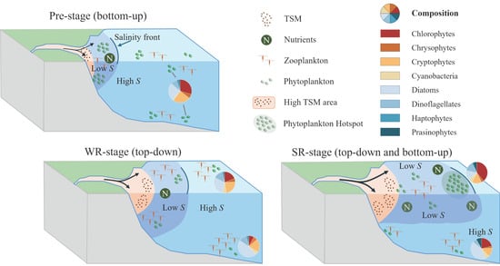
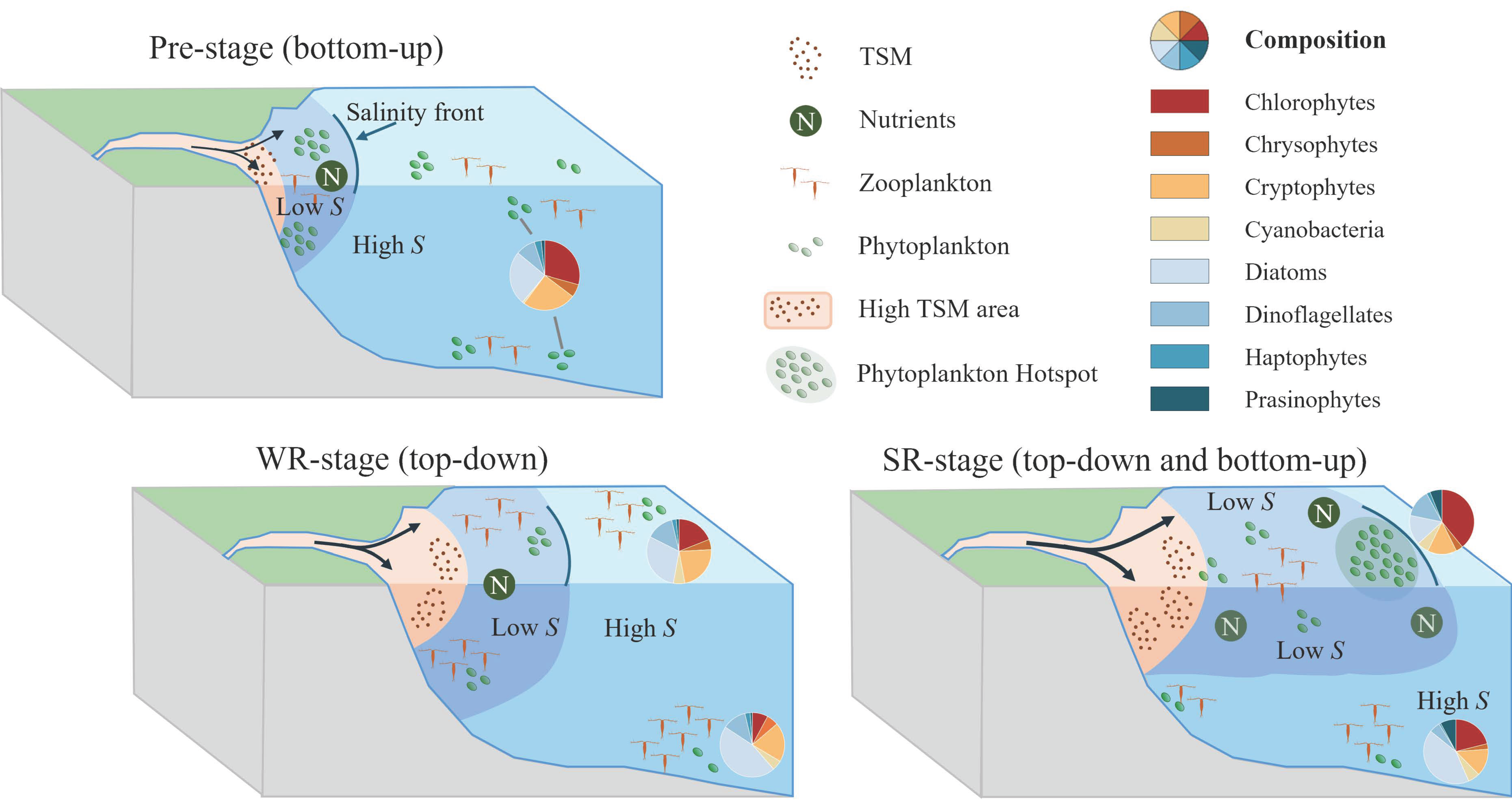
Graphical Abstract

1. Introduction

Estuaries are highly dynamic transition zones between rivers and oceans. They sustain diverse biological communities and fulfill critical ecological functions. In the past half-century, excessive inputs of land-derived nutrients have driven widespread eutrophication and recurrent phytoplankton blooms in estuarine ecosystems worldwide [1]. Numerous countries have implemented stringent nutrient management strategies, such as the Grizzle-Figg Act for Tampa Bay [2], Denmark’s Action Plan for the Aquatic Environment [3], the EU Water Framework Directive for European waters [4], and similar initiatives in Asia [5]. However, the response of estuarine algal blooms to nutrient reduction has been highly variable: while some systems (e.g., Tampa Bay) have shown significant declines [6], others (e.g., Chesapeake Bay, Baltic Sea) have exhibited persistent blooms due to internal nutrient cycling, food web restructuring, and climate change [7,8,9]. This variability makes effectively controlling estuarine algae bloom an urgent issue that is attracting increasing research attention [1,10].
Beyond chronic nutrient enrichment, episodic high-intensity nutrient pulses from seasonal runoff, hurricanes, or artificial floods can trigger large phytoplankton blooms and community shifts [11,12]. The Yellow River Estuary (YRE) exemplifies such a system. The Yellow River accounts for more than 75% of the total freshwater input of the Bohai Sea [13], but its discharge has declined markedly over the past half-century [13,14] (Figure S1A), accompanied by increased sediment deposition [15,16]. To mitigate sedimentation and improve downstream transport, the Water-Sediment Regulation Scheme (WSRS) has been implemented since 2002 [17]. This scheme uses synchronized reservoir operations to release short-term, high-volume discharges during summer, generating artificial flood pulses to flush accumulated sediment from downstream river channels. More than half of the annual nutrient flux of the YRE is discharged during the 2–3 weeks when WSRS is operational [18,19], fundamentally reshaping the physical and chemical habitat of phytoplankton in the YRE. However, its specific impacts on phytoplankton communities remain debated.
Phytoplankton dynamics are shaped by a combination of bottom-up controls, including nutrient availability, salinity, light, and temperature [20,21], and top-down controls, such as grazing pressure from zooplankton [22,23]. Most studies in YRE have focused on bottom-up drivers [24,25]. Early research suggested that the nutrient input during WSRS could replenish the nutrients depleted by the spring bloom, triggering a summer phytoplankton peak [19]. However, subsequent observations revealed that Chl a peaks consistently in September, not during the June–July WSRS, a phenomenon attributed to light limitation caused by WSRS-induced turbidity [26]. In contrast, top-down regulation via zooplankton grazing has been largely overlooked, although it is essential for elucidating the underlying mechanisms driving phytoplankton community dynamics [27,28,29,30]. Zhang et al. [31] observed a rapid increase in zooplankton biomass coinciding with the period of suppressed phytoplankton abundance during WSRS, suggesting that grazing pressure may exert a stronger influence than previously assumed. However, a comprehensive quantification of bottom-up versus top-down contributions during the WSRS is still lacking.
Furthermore, existing studies have predominantly relied on vertical hauls or focused solely on surface layer data [26,31,32], failing to capture the vertical dynamics of phytoplankton. The WSRS process features three distinct stages: pre-WSRS stage (low discharge and sediment load), water regulation (WR) stage (high discharge but low sediment load), and sediment regulation (SR) stage (high discharge and sediment load) (Figure S1C). Each stage has different hydrological conditions that create marked vertical gradient [33]. Therefore, surface and bottom layers may be governed by different environmental factors and ecological processes.
To understand the impact of the WSRS on the spatiotemporal distribution of phytoplankton communities in the YRE and the underlying driving mechanisms, we conducted three cruises during different WSRS stages in 2019 across five transects, corresponding to three distinct phases. We hypothesize that WSRS transitions phytoplankton regulation from predominantly bottom-up control during pre-WSRS stage to a more complex, vertically stratified regulatory framework during the WR and SR stages, with distinct drivers operating in surface versus bottom layers. This study aims to identify the stage- and layer-specific key factors controlling phytoplankton dynamics in the YRE, thereby elucidating the ecological effects of WSRS on phytoplankton distribution. The findings will provide a crucial basis for assessing estuarine ecological responses to episodic or pulses disturbances and for developing informed adaptive management strategies.

2. Materials and Methods

2.1. Study Area and Sampling Sites

The Yellow River Estuary, a typical temperate estuary in northern China, is characterized by shallow coastal waters, with depths generally <10 m in nearshore zones and ~20 m offshore (Table 1). Seasonal fluctuations in water and sediment discharge lead to pronounced physicochemical gradients [34,35]. During low-flow conditions, the influence of river discharge is restricted within the 10 m isobath. However, during the WSRS period, this influence on surface seawater can extend offshore to the central Bohai Sea [18,36]. In contrast, sediment input exerts a more localized effect, mostly concentrated near the river mouth, during low-flow periods and confined within the 10 m isobath during WSRS [18].
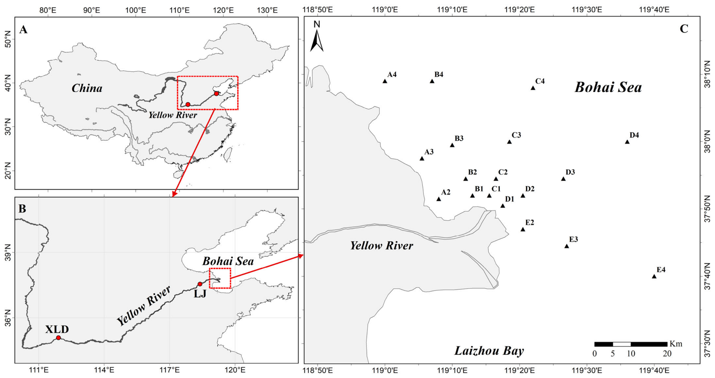
In 2019, the WSRS was conducted from 21 June to 2 August, with floodwater released from Xiaolangdi Reservoir Station. At Lijin Hydrological Station, a sharp increase in discharge (2430 m3 s−1) was recorded on 27 June, with corresponding hydrological impacts in the YRE observed 10 h later [26]. Sampling was conducted during three stages: 18–20 June (pre-WSRS stage), 5–7 July (WR stage) and 25–27 July (SR stage) (Figure S1C). During each stage, physical, chemical, and biological data were collected at 18 stations across five transects in the YRE (Figure 1C). However, during the SR stage, extremely high total suspended matter (TSM) concentrations in the bottom water near the river mouth caused immediate filter clogging. This prevented the collection of valid samples for pigment, nutrient, and other environmental parameter analyses. Consequently, no bottom data were obtained at the innermost coastal stations (A2, A3, B1, D1, E2) during this stage.

2.2. Sampling and Analysis Procedures

At each site, both surface and bottom samples were collected. Salinity and temperature were measured in situ using a Conductivity–Temperature–Depth (CTD) Profiler (RBRConcerto3, RBR Ltd., Ottawa, ON, Canada). Seawater samples were collected using Niskin bottles (KC-Denmark Company., Silkeborg, Region Midtjylland) for analysis of TSM, nutrients, and phytoplankton pigments. TSM was measured by the gravimetric method, following the Chinese National Standard (GB 17378.7-2007) [37]. Nutrient samples ( NO 3 , NO 2 , NH 4 + , PO 4 3 , and Si(OH)4) were filtered through 0.45 μm cellulose acetate filters and stored at –20 °C until laboratory analysis using an autoanalyzer (QuAAtro AutoAnalyzer 39, SEAL Analytical, Milwaukee, Wisconsin). Dissolved inorganic nitrogen (DIN) was calculated as the sum of NO 3 , NO 2 , and NH 4 + .
Zooplankton samples were collected using a 0.5 m diameter plankton net (505 μm mesh size) towed vertically at 0.5 m/s from 3 m above the seafloor to the surface. Samples were preserved in 5% buffered formalin and later identified and enumerated under a ZEISS Stemi 508 stereomicroscope (Carl Zeiss Microscopy GmbH, Hallbergmoos, Germany). Zooplankton biomass was calculated as wet weight per unit volume (μg L−1), following Chinese National Standard (GB 17378.7-2007) [37]. A piece of JF62 sieve mesh (Xiamen Dengxun Instrument Equipment Co., Ltd, Xiamen, China) was cut to fit the inner diameter of a funnel, wetted, and placed into the funnel. Excess water was removed using a vacuum pump, and the wet weight of the sieve mesh alone was recorded using an analytical balance with a precision of 0.0001 g for later calibration; this calibrated mesh could be reused for multiple samples. For sample measurement, the pre-calibrated sieve mesh was placed back into the funnel, and the vacuum pump was turned on. The zooplankton sample, from which large debris had been removed, was gently poured into the funnel. After all water had been filtered out, the vacuum pump was switched off. The sieve mesh together with the retained zooplankton was carefully taken out and placed on absorbent paper to remove superficial water. Finally, the mesh with the sample was weighed using the same balance, and the wet weight biomass of the zooplankton was obtained by subtracting the pre-recorded weight of the mesh.
Phytoplankton pigment samples were obtained by filtering 0.5–1 L of seawater onto 47 mm GF/F filters under low-light conditions. Filters were stored in cryovials immersed in liquid nitrogen. Pigments on frozen filters were extracted using 100% methanol. Filter pieces (≈2 × 5 mm) were transferred to 10 mL amber glass centrifuge tubes, to which 3 mL of methanol was added. The mixture was vortexed for 30 s and then extracted in an ice-water ultrasonic bath for 10 min. After filtration through a 0.2 µm PTFE syringe filter, water was added at a 1:5 (v/v) ratio to improve chromatographic peak shape. All steps were performed under dim light, and samples were analyzed immediately after preparation. Pigments were analyzed via high-performance liquid chromatography (HPLC), following the method of Zapata, Rodriguez, and Garrido [38], using a ZORBAX Eclipse XDB-C8 column (4.6 × 100 mm, 5 μm; Agilent Technologies, Newport, United States of America). Mobile phases consisted of eluent A (methanol–acetonitrile–0.25 M aqueous pyridine, 50:25:25, v:v:v) and eluent B (methanol–acetonitrile–acetone, 20:60:20, v:v:v). All the organic solvents were HPLC grade. The injection volume was 200 μL, and the flow rate was constant at 1 mL min−1. The temperature of the autosampler compartment was kept at 4 °C to inhibit the degradation of the pigments. Pigments were detected using diode-array spectroscopy (350–750 nm) and chlorophylls were additionally monitored by fluorescence (Ex 440 nm, Em 650 nm). Identification was achieved by co-chromatography with authentic standards. Pigment standards were provided by the DHI Institute for Water and Environment (Hørsholm, Denmark). Fourteen pigments, including fucoxanthin, 19-hex-fucoxanthin, peridinin, zeaxanthin, 19-but-fucoxanthin, alloxanthin, prasinoxanthin, lutein, diadinoxanthin, violaxanthin, neoxanthin, Chl a, and Chl b, were quantified.

2.3. Phytoplankton Composition Analysis

Phytoplankton biomass was measured in terms of Chl a concentration. The taxonomic composition of phytoplankton was inferred from pigment profiles using the CHEMTAX V1.95 [39]. The pigment/Chl a input ratio matrix included eight phytoplankton groups (Supplementary Table S1), based on regional studies [40,41]. To improve calculation stability, 60 randomized pigment/Chl a matrices were used as initial inputs, and the final results were obtained by averaging the six outputs with the lowest residuals [42].

2.4. Grazing Pressure

Zooplankton biomass (ZB) to Chl a concentration ratio (ZB/Chl a) has been widely applied as an index of top-down control potential in aquatic ecosystems [43,44]. Following these previous studies, we evaluated the potential grazing pressure (GP) of zooplankton using this biomass ratio, calculated as:
GP   =   Z B C h l   a
where ZB represents the zooplankton biomass (μg L−1), and Chl a denotes the concentration of Chl a (μg L−1). The GP is a dimensionless index that reflects the relative grazing pressure at each sampling site. Higher GP values indicate potentially stronger top-down control by zooplankton on phytoplankton, whereas lower GP values suggest weaker grazing pressure or higher phytoplankton biomass relative to grazer biomass. The GP was calculated separately for the surface and bottom layers at each site, using the station-specific ZB paired with the corresponding depth-specific Chl a concentration from each layer.

2.5. Statistical Analysis

Independent two-sample t-tests were employed to analyze variations in Chl a across the three WSRS stages within the two water layers (surface and bottom). The analysis was conducted separately for each layer, with all possible pairwise comparisons among stages (pre-WSRS vs. WR, WR vs. SR, SR vs. pre-WSRS) performed independently for each layer. Analysis of similarities (ANOSIM) was performed to assess the significance of differences in phytoplankton community composition across stages and layers. The analysis was based on a Bray–Curtis dissimilarity matrix derived from Hellinger-transformed species abundance data. The test yields an R statistic (Version 4.5.3) ranging from −1 to 1, where values close to 1 indicate strong separation between groups (i.e., dissimilarities between groups exceed those within groups), while an R value close to 0 suggests minimal separation. Statistical significance was assessed using 999 permutations, with results considered significant at p < 0.05. Post hoc pairwise comparisons were conducted when significant global differences were detected, with p-values adjusted using the Bonferroni correction to account for multiple testing.
Regression tree analysis was applied to assess the relative importance of top-down and bottom-up controls on phytoplankton abundance (represented by Chl a concentration) and to identify the relationships between driver variables (environmental factors and grazing pressure) and the response variables (Chl a concentration), following the approach outlined by [45]. Spearman’s correlation analysis was conducted to address collinearity among driver variables. Variables with Spearman’s coefficients |ρ| > 0.5 (p < 0.05) were excluded to ensure independence and avoid collinearity issues in the final model [45]. Given the significant correlations among DIN, salinity, and Si(OH)4 in the surface layer across all stages, DIN and Si(OH)4 were excluded in the pre-WSRS stage based on its significant correlation with temperature (Spearman’s coefficients ρ = −0.71, p < 0.05; Supplementary Figure S1). In the SR stage, both DIN and Si(OH)4 were excluded due to their significant correlations with temperature (Spearman’s coefficients ρ = −0.88, p < 0.01) and salinity (Spearman’s coefficients ρ = −0.86, p < 0.05), respectively (Supplementary Figure S1).
Before running the regression tree analysis, the distributions of all response and driver variables were tested for skewness using Pearson’s skewness coefficient in SPSS 22.0. Non-normally distributed variables were log-transformed using log10(x + 1) to reduce skewness and ensure normality for model accuracy. Separate regression tree analyses were performed for Chl a at different stages. In each tree, a minimum of six samples per leaf node was set, and the maximum tree depth was limited to two to prevent overfitting and ensure a simpler, more interpretable model. Cross-validation with 10-fold and 1000 repetitions was used to ensure model generalization and further avoid overfitting.
Redundancy analysis (RDA) was performed to quantify the relationships between the selected driver variables and phytoplankton community composition. RDA was selected based on detrended correspondence analysis results, showing the maximum gradient length of the first axis to be between 3 and 4, indicating a linear response for RDA. Prior to the analysis, abundance data of phytoplankton groups were Hellinger-transformed to reduce the influence of highly abundant species and allow for the use of a linear-based method. The selected driver variables were standardized (z-score) to eliminate the effects of differing units and scales. The transformed phytoplankton group data constituted the response matrix, while the standardized driver variables constituted the explanatory matrix.
Independent two-sample t-tests, ANOSIM analysis, and regression tree analysis were performed using R version 4.5.3. The ‘ggsignif’ package (Version 0.6.4) was used for t-tests, the ‘vegan’ package (Version 2.7.2) for ANOSIM analysis, the ‘rpart’ package (Version 4.1.24) was used for regression tree analysis, and the ‘ggplot2’ package (Version 4.0.3) was used for statistical visualization. The RDA was conducted using CANOCO version 5. Contour figures were created using Surfer version 15, while distribution figures were created using ArcGIS version 10.3.

3. Results

3.1. Spatial and Temporal Variation in Driver Variables

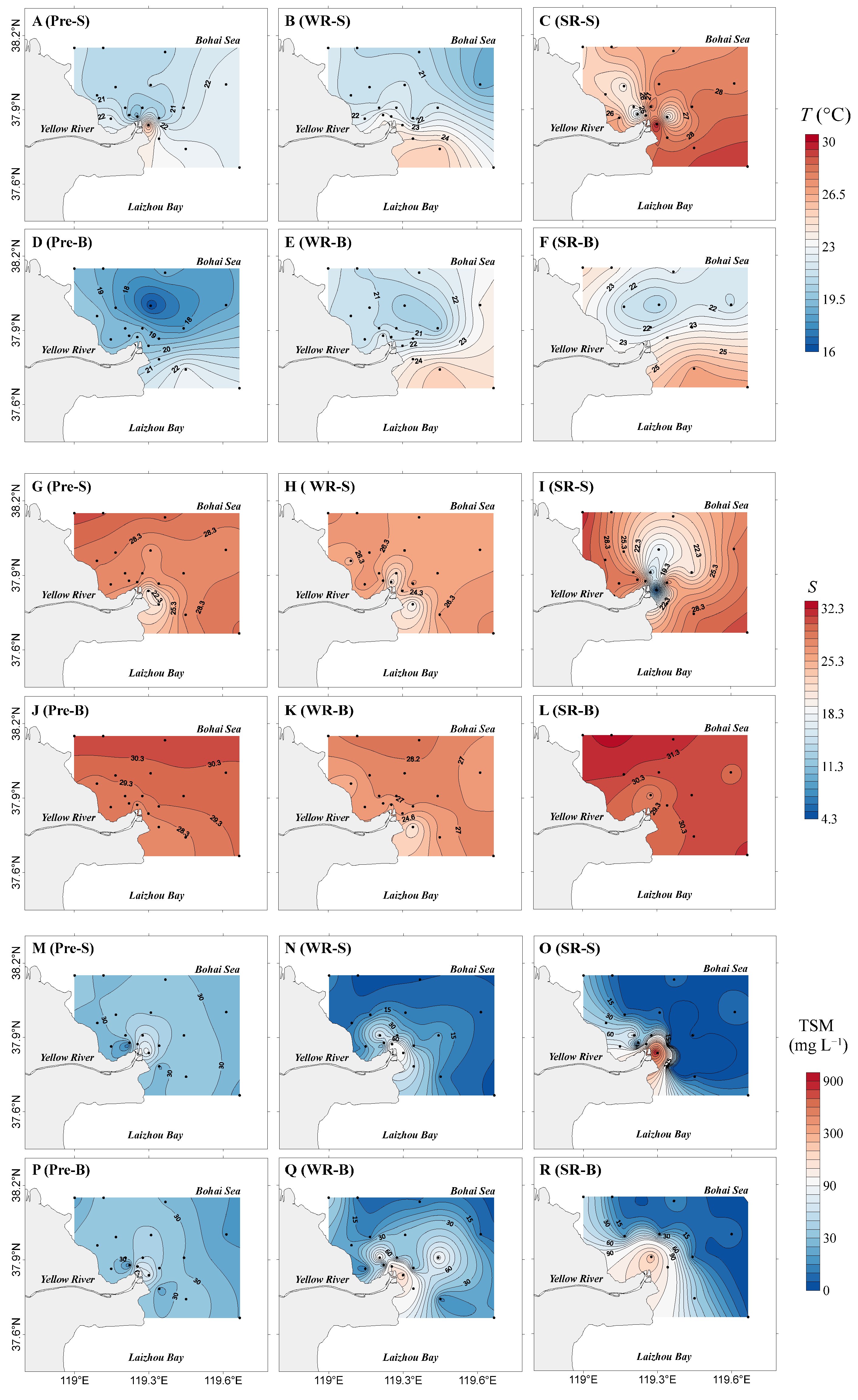
Surface water temperature exhibited a pronounced latitudinal gradient across all three stages (Figure 2A–C), with the highest temperature (30.2 °C) recorded in the southeast during the SR stage (Table 2). Bottom water temperature showed a similar latitudinal gradient to the surface (Figure 2D–F), but the surface–bottom temperature difference increased markedly during the SR stage, particularly in the northern offshore area. Surface salinity increased seaward from the river mouth in all stages, with the low-salinity region (<25) expanding under enhanced freshwater discharge during the WSRS (Figure 2G–I). Bottom salinity was consistently higher than at the surface, with low-salinity waters confined to the vicinity of the river mouth (Figure 2J–L). Surface total suspended matter (TSM) followed an opposite pattern to salinity, peaking around the river mouth during the SR stage (Figure 2M–O). Bottom TSM exhibited a distribution similar to the surface, but with a broader high-value area and a lower maximum during the WR and SR stages (Figure 2P–R).
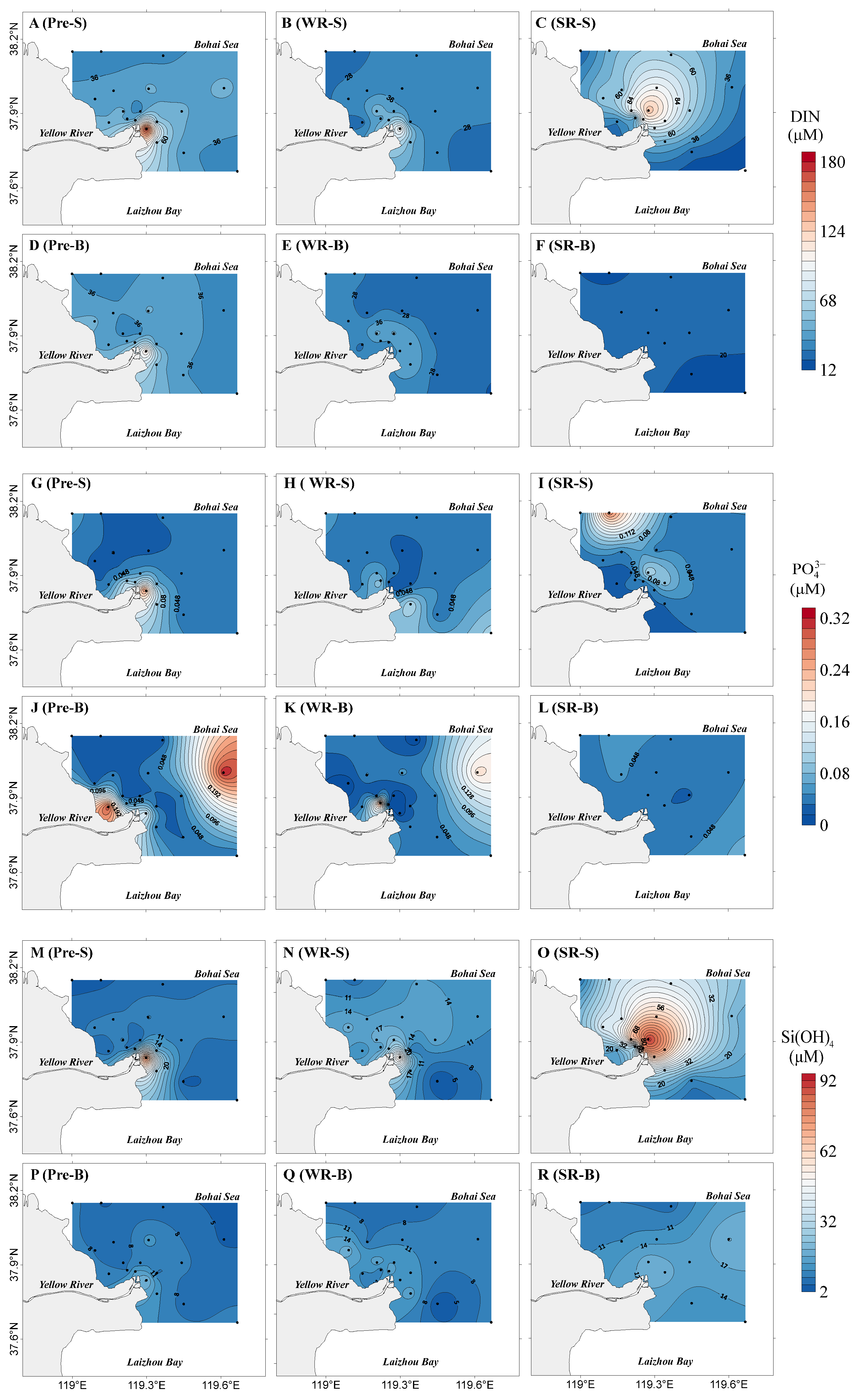
High nitrate and silicon concentrations and low phosphate concentrations were observed at all stages, with surface waters consistently higher than bottom layers (Table 2, Figure 3). During the pre-WSRS stage, the highest nutrient concentrations were found around the river mouth (Figure 3A,D,G,M,P), except for bottom PO 4 3 , which peaked in the offshore northeastern area (Figure 3J). During the WR stage, nutrient concentrations decreased sharply, but nutrient distributions were similar to those in the pre-WSRS stage (Figure 3B,E,H,K,N,Q). In the SR stage, the vertical differences in nutrient concentrations became more pronounced. At the surface, the high-concentration areas of DIN and Si(OH)4 shifted northeastward, peaking at station C2 (Figure 3C,O), whereas the highest PO4 concentrations occurred in the northwestern part of the study area (Figure 3I). In contrast, bottom-layer nutrients exhibited smaller spatial variations, with all three nutrients remaining at relatively low levels (Figure 3F,L,R).
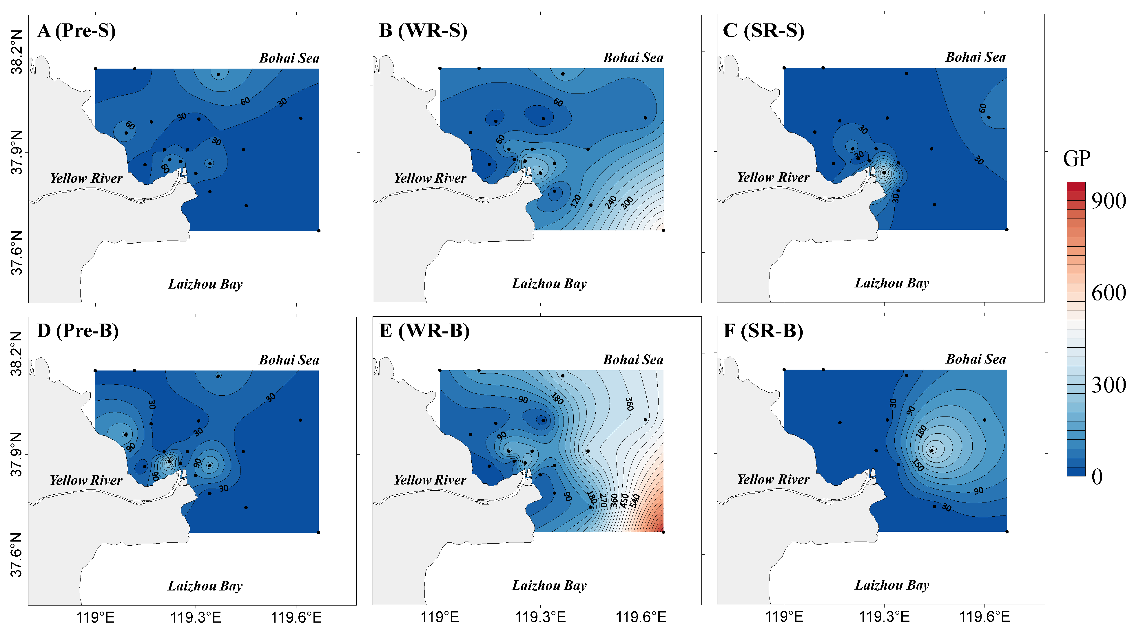
Grazing pressure increased from the pre-WSRS stage to the WR stage, followed by a sharp decline during the SR stage (Table 2). Grazing pressure was consistently higher in the bottom layer than surface layer at all stages (Figure 4). During the pre-WSRS stage, areas with higher grazing pressure were located near the river mouth and in the northern part of the study area in both surface and bottom layers, largely coinciding with high nutrient regions (Figure 4A,D). During the WR stage, the grazing pressure increased approximately threefold, accompanied by a seaward shift and southeastward expansion of the high-value zone in surface and bottom layers (Figure 4B,E). In the SR stage, grazing pressure returned to pre-WSRS levels, with elevated grazing zones located near the river mouth in the surface layer and in the offshore eastern region in the bottom layer (Figure 4C,F).

3.2. Spatial and Temporal Variation in Phytoplankton Community

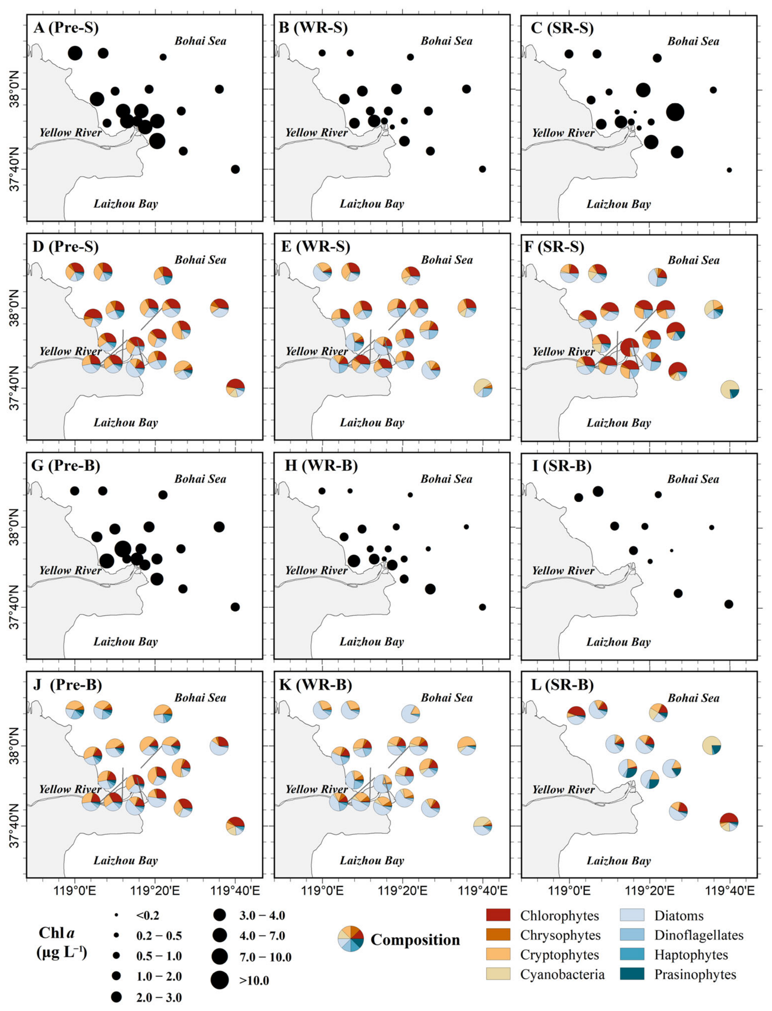
Phytoplankton abundance, represented by Chl a concentration, exhibited different patterns between surface and bottom waters. In the surface layer, Chl a decreased significantly from 3.32 ± 1.99 μg L−1 during the pre-WSRS stage to 1.58 ± 0.89 μg L−1 during the WR stage (t-test, p < 0.01, Figure S3a), followed by a recovery to 2.36 ± 3.09 μg L−1 during the SR stage (Table 2). In contrast, Chl a in the bottom layer decreased significantly during both the WR and SR stage (t-test, p < 0.01 for both stages, Figure S3b). Specifically, the mean value dropped from 2.68 ± 1.50 μg L−1 in the pre-WSRS stage to 1.22 ± 0.86 μg L−1 in the WR stage and further declined to 1.05 ± 0.71 μg L−1 in the SR stage (Table 2). Meanwhile, phytoplankton community composition was significantly altered in both layers (ANOSIM analysis, R = 0.135, 0.336, p = 0.001 for both surface and bottom layers, Figure S3c,d).
During the pre-WSRS stage, Chl a concentration was higher near the river mouth in the surface layer, where chlorophytes, cryptophytes, and diatoms dominated the phytoplankton community (Figure 5A,D). The spatial distribution of Chl a and the community composition in the bottom layer were similar to those in the surface layer (Figure 5G,J). During the WR stage, Chl a concentration decreased significantly in both the surface and bottom layers, particularly near the river mouth (Figure 5B,H). The proportion of chlorophytes decreased in both layers, while dinoflagellates increased in the surface layer and diatoms became more dominant in the bottom layer. During the SR stage, a distinct high-Chl a zone formed around site D3 in the surface layer, with Chl a concentration reaching 6.8 fold higher than the pre-WSRS level (Figure 5C). In this zone, chlorophytes accounted for over 54% of the total Chl a. Interestingly, the high-concentration zone in the surface layer corresponded to a low-concentration zone in the bottom layer, where diatoms, cryptophytes, and prasinophytes dominated the phytoplankton community (Figure 5L).

3.3. Alternating Dominance of Bottom-Up and Top-Down Control

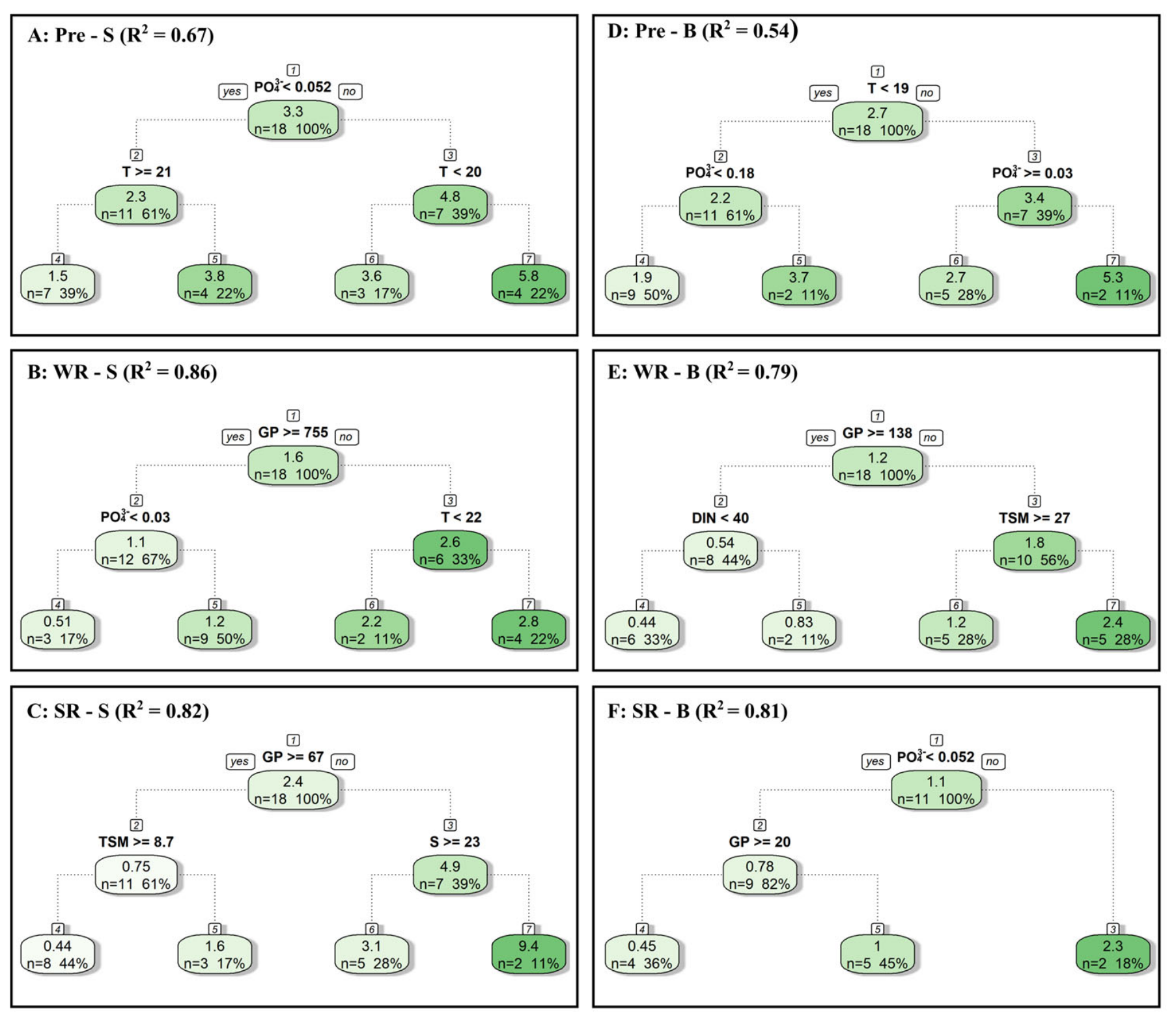
We performed regression tree analyses on Chl a concentration to identify the stage-specific dominant mechanisms regulating phytoplankton dynamics. The results revealed stage- and layer-specific shifts in the primary drivers of Chl a (Figure 6).
Figure 6. Regression tree results for Chl a of both layers during each WSRS stage. The R2 value indicates the proportion of variance explained by the primary controlling factor (i.e., the first split in the tree). The terms Pre-, WR-, and SR-correspond to the pre-WSRS, WR, and SR stages, combined with -S or -B to specify the surface and bottom layer. This nomenclature is consistent with Figure 7.
Water 18 01283 g006
During the pre-WSRS stage, Chl a dynamics were primarily regulated by bottom-up controls. The initial split of the regression tree indicated that PO4 concentration and temperature were the main drivers in the surface and bottom layers, respectively (Figure 6A,D). Normalized importance (NI) analysis further supported the importance of these two factors, with PO4 contributing 29% in the surface layer and 41% in the bottom layer, while temperature accounted for 26% and 18%, respectively (Table 3). During the WR stage, the system shifted towards a top-down dominated regime. The first split identified grazing pressure as the key factor constraining Chl a levels of both layers (Figure 6B,E). This was strongly reflected in the normalized importance, where grazing pressure explained 64% of the variation in the surface layer and 31% in the bottom layer (Table 3). During the SR stage, the regulatory mechanisms diverged between layers. While the surface layer remained under top-down control (first split: grazing pressure; NI = 38%), the bottom layer transitioned to a bottom-up control, with PO4 concentration identified as the dominant driver in both the initial split and normalized importance (Figure 6C,F; Table 3). Notably, salinity emerged as another key factor (second split) in the surface layer during this stage (Figure 6C), accounting for 40% of the total explained variation (Table 3).

3.4. Relationship Between Driver Variables and Phytoplankton Community

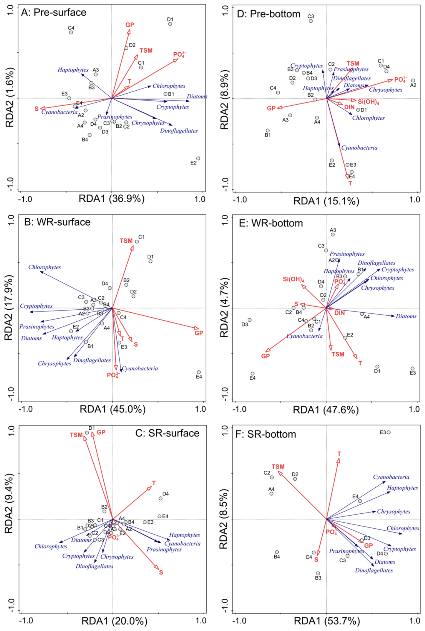
We performed RDA to investigate relationships between phytoplankton groups (blue lines in Figure 7) and driver variables (red lines in Figure 7) at different WSRS stages.
During the pre-WSRS stage, the first two axes of the surface layer explained 36.9% and 1.6% of the variation, respectively (Figure 7A). The first axis was mainly associated with PO4 concentration and salinity, while the second axis was primarily influenced by grazing pressure. The dominant phytoplankton groups, chlorophytes, cryptophytes, and diatoms, collectively showed a strong association with high PO4 concentrations and low salinity conditions. In the bottom layer, the first two axes explained 15.1% and 8.9% of the variation, respectively (Figure 7D). Here, the first axis was mainly associated by PO4 concentration and grazing pressure, while the second axis was influenced primarily by seawater temperature. In contrast to the surface layer, the key environmental drivers of the dominant phytoplankton groups were more differentiated. Chlorophytes exhibited a positive correlation with DIN and Si(OH)4 concentration. Diatoms, however, were primarily governed by PO4 concentration (positive) and grazing pressure (negative). Cryptophytes were predominantly negatively correlated with temperature.
During the WR stage, the first two axes of the RDA for the surface layer explained approximately 45.0% and 17.9% of the variation (Figure 7B). The first axis was mainly associated with grazing pressure, while the second axis was primarily associated with TSM and PO4. Chlorophytes, cryptophytes, and diatoms, which were the dominant phytoplankton groups in the surface layer, were inversely related to grazing pressure. Cyanobacteria, which increased markedly in offshore regions, were predominantly regulated by TSM (negative) and PO4 (positive). In the bottom layer, the first two axes explained 47.6% and 4.7% of the variation, respectively, with both axes primarily shaped by grazing pressure (Figure 7E). Most phytoplankton groups demonstrated a significant negative correlation with grazing pressure, while cyanobacteria displayed a positive correlation with grazing pressure. In contrast, diatoms with high dominance were associated with low salinity and high Si(OH)4 concentrations.
During the SR stage, the first axis of the RDA for the surface layer, which accounted for 20% of the total variation, was mainly contributed by salinity (Figure 7C). The second RDA axis, explaining 9.4% of the variation, was primarily driven by TSM and grazing pressure (Figure 7C). Phytoplankton groups in the surface layer exhibited two distinct response patterns to environmental variables. Haptophytes, cyanobacteria, and prasinophytes were associated with high salinity and low TSM and grazing pressure levels. The other groups were related to low temperature. In the bottom layer, the first two axes explained 53.7% and 8.5% of the variation, respectively (Figure 7F). The first axis was mainly contributed by grazing pressure and TSM concentration (negative), while the second axis was primarily contributed by temperature. Diatoms, chlorophytes, cryptophytes, and prasinophytes, which were the dominant phytoplankton groups in the bottom layer, exhibited negative correlations with grazing pressure.

4. Discussion

Our study demonstrates that WSRS drives a stage-specific shift in the dominant control mechanisms regulating phytoplankton: from bottom-up control governed primarily by resource availability during the pre-WSRS stage, through top-down control dominated by grazing pressure during the WR stage, culminating in a trophic–physical coupled regulation in the surface layer alongside persistent resource limitation in the bottom layer during the SR stage. This mechanistic shift not only alters the spatial distribution of phytoplankton, leading to the formation of an anomalous high-abundance zone in the surface layer during the SR stage, but also profoundly reshapes community structure. Below, we first explore how this shift in control mechanisms drives phytoplankton redistribution, followed by an analysis of the responsive and adaptive strategies of the phytoplankton community.

4.1. Bottom-Up vs. Top-Down Control Driving Phytoplankton Distribution During WSRS

While most studies agree that phytoplankton do not show a generalized increase during WSRS, the governing mechanisms remain debated. Some attribute the phytoplankton distribution to bottom-up control, such as reduced light availability and mechanical damage, which offset the impact of high nutrient input [26,46]. Zhang et al. [31] suggests that a rapid increase in zooplankton abundance during WSRS enhances top-down control, thereby suppressing phytoplankton stock. Our study indicates that phytoplankton distribution in the YRE during WSRS is co-regulated by grazing (top-down) and resource availability (bottom-up) controls, with their relative importance shifting across water layers and WSRS stages.
During the pre-WSRS stage, phytoplankton abundance was highest around the nutrient-rich river mouth in both surface and bottom layers. Its distribution was dominated by bottom-up control, with PO4 concentration and temperature serving as the primary factors in the surface and bottom layers, respectively. Stable hydrological conditions and weak grazing pressure gave rise to a resource-controlled equilibrium, where estuarine productivity was governed by proximity to the freshwater source (nutrients source) [47,48].
During the WR stage, phytoplankton abundance declined sharply in both layers, with regression tree models indicating a shift from bottom-up to top-down control dominance. This result confirms the crucial role of zooplankton grazing in regulating phytoplankton abundance [49,50,51]. Although large nutrient inputs from high freshwater discharge stimulated phytoplankton growth [19,52], a concomitant surge in zooplankton populations rapidly offset this growth through intense grazing pressure [53], in turn resulting in suppressed Chl a concentration. Although phytoplankton grazing clearance rates were not measured in this study, investigations in similar estuaries have reported clearance rates exceeding 0.5 d−1 during high discharge seasons [50]. Additionally, nutrient concentrations did not rise proportionally with discharge, further indicating rapid phytoplankton turnover. This pattern mirrors observations in the monsoon-driven Arabian Sea, where high freshwater and nutrient inputs coincide with strong zooplankton recruitment but low phytoplankton biomass [54] and aligns with other aquatic ecosystems where top-down control overrides bottom-up stimulation under strong environmental forcing [55,56]. Similar grazing regulation has been documented in Baltic Sea lagoons: in the Vistula Lagoon, zooplankton consumed ~28% of the phytoplankton standing stock, reducing algal blooms [57]; in the Curonian Lagoon, microzooplankton removed up to 78% of nanophytoplankton standing stock [58]. These findings support our conclusion that top-down control can override bottom-up stimulation under strong hydrological forcing, suggesting such regulation is widespread in estuarine and lagoon ecosystems.
During the SR stage, phytoplankton abundance recovered but with enhanced spatial heterogeneity, marked by a low-value area around the estuary and a distinct high-biomass zone in the surface layer. Top-down control persisted in the surface layer, while bottom-up control dominated in the bottom layer. The low phytoplankton zone around the river mouth is likely due to elevated turbidity caused by sediment discharge, which reduced light availability and inhibited phytoplankton growth [26,59,60], with the effect usually geographically constrained by the sediment front [61,62]. The phytoplankton hotspot in the surface layer can be explained by a trophic–physical framework. First, persistent freshwater input formed a stratified frontal zone that concentrated river-derived nutrients via convergence and lateral supply, creating a biological hotspot [63]. Second, the sharp physical gradient at the salinity front may trigger behavioral avoidance by zooplankton [64,65,66], locally creating a zone of reduced predator efficiency [67]. This allowed phytoplankton to escape predation in this resource-rich refuge and accumulate biomass, potentially elevating summer bloom risk in the YRE.
Based on the above analysis, we propose a conceptual framework synthesizing the stage-specific shifts in regulatory mechanisms and their cascading effects on phytoplankton distribution during WSRS. This framework illustrates how the interplay between bottom-up control, top-down control, and physical processes varies across water layers and WSRS stages, ultimately shaping the spatial heterogeneity of phytoplankton biomass and community structure in the YRE.

4.2. WSRS Reshape Phytoplankton Community Composition in the YRE

Phytoplankton communities are highly diverse in size, physiology, and environmental tolerances, making their composition more sensitive to changes in environmental conditions and grazing pressures than bulk indicators such as Chl a and total abundance [22,68,69]. In our study, community composition varied markedly across WSRS stages, especially around the river mouth where WSRS influence is most pronounced, consistent with prior findings in the YRE [31,32]. Notably, compositional shifts were more pronounced in the bottom layer than in the surface layer, suggesting that WSRS may exert a stronger influence on community structure than on horizontal distribution patterns.
Prior to the WSRS, Chl a peaked in both surface and bottom layers around the river mouth, with vertically homogeneous communities dominated by chlorophytes, cryptophytes, and diatoms. RDA indicated these groups were negatively correlated with salinity and positively correlated with nutrient levels in the surface layer. Their dominance was likely due to their efficient nutrient uptake and rapid growth rates in resource-rich environments, making them strong competitors in undisturbed estuaries [70,71]. In the bottom layer, cryptophytes correlated with lower temperatures, whereas diatoms and chlorophytes were positively linked to nutrient concentrations and negatively associated with grazing pressure. The dominance of cryptophytes may be attributed to their competitive advantage under cooler conditions [72], while the dominance of diatoms and chlorophytes highlights their resource-driven growth and defensive capabilities [71]. Diatoms are protected by their siliceous frustules (physical defense), whereas chlorophytes rely on rapid growth (r-selected strategy) to offset grazing mortality [73].
During the WR stage, the massive freshwater input delivered abundant nutrients but simultaneously triggered sharp declines in salinity, increased turbidity, and intensified zooplankton grazing [19,31]. These changes drove clear vertical differentiation in phytoplankton communities. In the surface layer, chlorophytes, cryptophytes, and diatoms remained dominant, while chlorophytes decreased and dinoflagellates increased in relative abundance. The strong negative correlation of chlorophytes with grazing pressure suggests their decline results from preferential grazing by copepods, the dominant zooplankton in the YRE [74], which selectively consume chlorophytes [70,75]. In contrast, the increase in dinoflagellates can be attributed to their motility and mixotrophic capability, enabling behavioral avoidance of grazers and nutritional flexibility under combined light and grazing stress [76,77]. In the bottom layer, most groups declined sharply, especially chlorophytes and cryptophytes, reflecting heightened vulnerability when growth is already hampered by low light [73]. This is supported by RDA, showing significant negative correlations with grazing pressure and TSM. Conversely, diatoms increased markedly, likely due to their competitive advantages under fluctuating light [78] and frustule-based grazing resistance [79], consistent with their weaker negative correlation with grazing pressure in RDA.
During the SR stage, increased sediment discharge and freshwater inputs elevated TSM concentration around the river mouth and formed a low-salinity surface layer, maintaining pronounced vertical differences in phytoplankton composition. This difference was primarily driven by salinity-induced physical structuring and reduced grazing pressure. In the surface layer, the stable structure combined nutrient retention, improved light availability, and grazing release, allowing fast-growing chlorophytes to form localized biomass hotspots [71]. Consistent with this, RDA showed no significant correlation between chlorophytes and grazing pressure, suggesting a shift in their regulatory mechanism from top-down regulation (dominant during WR stage) to bottom-up control by resource. In the bottom layer, diatoms remained dominant, whereas chlorophytes and cryptophytes declined markedly, and cyanobacteria together with prasinophytes increased in proportion. Diatoms, prasinophytes, and cyanobacteria thrived, owing to adaptive traits, such as low light acclimation, grazing-resistant structures, and nitrogen fixation, which enabled them to persist through high-grazing conditions during the WR stage and outcompete other groups during the SR stage [80]. In contrast, chlorophytes and cryptophytes, which are highly grazing-sensitive and nutrient-dependent [81,82], failed to recover from WR stage depletion under persistent light and nutrient limitation.

4.3. Study Limitations

Several limitations should be acknowledged. First, our study employed a Plankton Net I (mesh size of 505 µm) to collect zooplankton samples, focusing on medium- to large-sized zooplankton. As a result, the contribution of smaller zooplankton was not accounted for when estimating the strength of top-down effects based on zooplankton biomass. However, global estimates using the grazing dilution technique [83] indicate that microzooplankton (<200 µm) contribute significantly to phytoplankton consumption [23,84,85]. Therefore, in terms of microzooplankton, the exclusions of our study may have led to an underestimation of the strength of top-down control. Zooplankton were collected using vertical net tows that integrate the entire water column. Because the study area is shallow (<20 m) and characterized by strong vertical mixing due to wind and tides, depth-integrated sampling provides a reasonable representation of the bulk zooplankton community [86]. However, some vertical heterogeneity may still exist. Future studies should employ stratified water samplers or depth-discrete net tows to more precisely assess variations in grazing pressure across different water layers.
Second, our grazing pressure metric, calculated as the ratio of zooplankton biomass to Chl a concentration, provides a relation index rather than direct grazing rates. This metric was derived without excluding non-herbivorous taxa (e.g., chaetognaths) and distinguishing live and dead individuals. Although this ratio is a standard and widely used indicator of relative grazing pressure in aquatic ecosystems [43,44], it must be noted that including predatory zooplankton (which do not directly graze on phytoplankton) and dead individuals in biomass estimates may lead to systematic overestimation of grazing pressure [87]. This concern is particularly relevant in dynamic estuarine environments characterized by elevated turbidity and fluctuating salinity, where zooplankton mortality can be substantial [88,89]. Future studies should therefore combine improved grazing pressure estimates (e.g., functional group classification, grazing experiments, vital staining) with higher-resolution phytoplankton identification (e.g., microscopy or metabarcoding) to better understand how top-down and bottom-up mechanisms jointly shape phytoplankton community responses to WSRS.
Third, our temporal resolution, three discrete sampling events may not fully capture the continuous transitions between WSRS stages, particularly the rapid shifts in zooplankton and phytoplankton populations. Our study focused on the immediate YRE region; extending spatial coverage to adjacent Bohai Sea waters could better contextualize the offshore extent of WSRS influences. Despite these limitations, our multi-stage, layer-specific approach provides critical insights into the complex regulatory mechanisms governing phytoplankton responses to high-intensity hydrological disturbances.

5. Conclusions

In this study, we elucidated how the WSRS reshapes phytoplankton community structure and distribution in the Yellow River Estuary. Our findings demonstrate three main conclusions. First, WSRS-induced changes in water, sediment, and nutrient fluxes drive a progressive shift in the estuarine ecosystem: from an initial resource driven state, through a consumer dominated phase, to a physically biologically coupled state. This transition amplifies spatial heterogeneity between surface and bottom layers. Second, under intensive short-term disturbances, top-down control (e.g., grazing pressure) and physical stressors (e.g., light limitation, stratification) can rapidly override nutrient inputs, becoming the dominant forces shaping phytoplankton distribution. Third, environmental factors such as salinity and temperature not only act as direct resources or stressors but also indirectly modulate the relative strength of top-down and bottom-up processes by creating physical heterogeneity. These findings challenge the traditional nutrient centric paradigm for estuarine eutrophication management and underscore the need to integrate hydrological physical processes and food web dynamics into future environmental frameworks.

Supplementary Materials

The following supporting information can be downloaded at https://www.mdpi.com/article/10.3390/w18111283/s1: Table S1: Chl a ratios used in CHEMTAX analysis of pigment data; Table S2: List of zooplankton taxa and their occurrence during the pre-WSRS, WR-stage, and SR-stage; Table S3 Dominant zooplankton species across pre-WSRS, WR-stage, and SR-stage; Figure S1: Fresh water and sediment discharge at Lijin Station, A: annual data; B: monthly for 2019; C: daily data from June to August for 2019. Figure S2: Spearman’s correlations among all driver variables at different stages; Figure S3: Comparison analysis of phytoplankton abundance (in terms of Chl a concentration) and community across WSRS stages.

Author Contributions

Y.W.: methodology, formal analysis, writing—original draft; J.W.: data curation, formal analysis, visualization; R.S.: investigation, resources, project administration; W.Q.: writing—review and editing, validation; Z.L.: conceptualization, writing—review and editing; J.Z.: supervision, conceptualization, funding acquisition. All authors have read and agreed to the published version of the manuscript.

Funding

This paper was supported by the National Natural Science Foundation of China (Grant No. 42306163), and the Shandong Provincial Natural Science Foundation (Grant No. ZR2022MD079).

Data Availability Statement

The data presented in this study are available in the Supplementary Materials.

Acknowledgments

We would like to thank Bingqing Xu and Shaowen Li from Shandong Marine Resource and Environment Research Institute for their assistance during the sample collection. We would like to thank Henry H. Hansen from Karlstad University for manuscript editing and language improvements. We also thank Enhui Wang from the Yantai Standard Measurement Inspection Center for his support in pigment sample measurements.

Conflicts of Interest

Author Ruiting Shen was employed by Water Transportation Planning and Design Institute under CCCC (China Communications Construction Water Transportation Consultants Co., Ltd.). The remaining authors declare that the research was conducted in the absence of any commercial or financial relationships that could be construed as potential conflicts of interest.

Abbreviations

The following abbreviations are used in this manuscript:
WSRSWater-Sediment Regulation Scheme
YREYellow River Estuary
Chl aChlorophyll a
SRSediment Regulation (stage)
WRWater Regulation (stage)
RDARedundancy Analysis
TSMTotal Suspended Matter
DINDissolved Inorganic Nitrogen
CTDConductivity–Temperature–Depth
HPLCHigh-Performance Liquid Chromatography
PTFEPolytetrafluoroethylene (PTFE syringe filter)
GPGrazing Pressure
ANOSIMAnalysis of Similarities
NINormalized Importance
MSEMean Squared Error

References

  1. Dai, Y.; Yang, S.; Zhao, D.; Hu, C.; Xu, W.; Anderson, D.M.; Li, Y.; Song, X.P.; Boyce, D.G.; Gibson, L.; et al. Coastal phytoplankton blooms expand and intensify in the 21st century. Nature 2023, 615, 280–284. [Google Scholar] [CrossRef]
  2. Greening, H.; Janicki, A.; Sherwood, E.T.; Pribble, R.; Johansson, J.O.R. Ecosystem responses to long-term nutrient management in an urban estuary: Tampa Bay, Florida, USA. Estuar. Coast. Shelf Sci. 2014, 151, A1–A16. [Google Scholar] [CrossRef]
  3. Riemann, B.; Carstensen, J.; Dahl, K.; Fossing, H.; Hansen, J.W.; Jakobsen, H.H.; Josefson, A.B.; Krause-Jensen, D.; Markager, S.; Stæhr, P.A.; et al. Recovery of Danish Coastal Ecosystems After Reductions in Nutrient Loading: A Holistic Ecosystem Approach. Estuaries Coasts 2016, 39, 82–97. [Google Scholar] [CrossRef]
  4. WWF European Policy Office. The EU Water Framework Directive: A Modern and Powerful Tool to Provide Clean, Healthy, Flowing Waters; Living Rivers Europe: Brussels, Belgium, 2025. [Google Scholar]
  5. Water Environmental Partnership in Asia. Outlook on Water Environmental Management in Asia 2018; Retrieved 3 November 2024; Ministry of the Environment: Tokyo, Japan, 2018.
  6. Andersen, J.H.; Carstensen, J.; Conley, D.J.; Dromph, K.; Fleming-Lehtinen, V.; Gustafsson, B.G.; Josefson, A.B.; Norkko, A.; Villnäs, A.; Murray, C. Long-term temporal and spatial trends in eutrophication status of the Baltic Sea. Biol. Rev. 2017, 92, 135–149. [Google Scholar] [CrossRef] [PubMed]
  7. Harding, L.W.; Mallonee, M.E.; Perry, E.S.; Miller, W.D.; Adolf, J.E.; Gallegos, C.L.; Paerl, H.W. Long-term trends, current status, and transitions of water quality in Chesapeake Bay. Sci. Rep. 2019, 9, 6709. [Google Scholar] [CrossRef] [PubMed]
  8. Paerl, H.W.; Valdes, L.M.; Piehler, M.F.; Stow, C.A. Assessing the Effects of Nutrient Management in an Estuary Experiencing Climatic Change: The Neuse River Estuary, North Carolina. Environ. Manag. 2006, 37, 422–436. [Google Scholar] [CrossRef]
  9. de Beer, E.C.; Adams, J.B.; Lemley, D.A. Documenting phytoplankton community responses to hydrological resetting events in eutrophic low-inflow estuaries. Mar. Environ. Res. 2025, 211, 107399. [Google Scholar] [CrossRef] [PubMed]
  10. Sakamoto, S.; Lim, W.A.; Lu, D.; Dai, X.; Orlova, T.; Iwataki, M. Harmful algal blooms and associated fisheries damage in East Asia: Current status and trends in China, Japan, Korea and Russia. Harmful Algae 2021, 102, 101787. [Google Scholar] [CrossRef] [PubMed]
  11. Wetz, M.S.; Paerl, H.W. Estuarine Phytoplankton Responses to Hurricanes and Tropical Storms with Different Characteristics (Trajectory, Rainfall, Winds). Estuaries Coasts 2008, 31, 419–429. [Google Scholar] [CrossRef]
  12. Li, H.; Li, S.; Zhang, M.; Li, X.; Xu, Z.; Ma, H.; Liang, S.; Song, D.; Li, J.; Ma, Y.; et al. Typhoon-induced stormwater drives nutrient dynamics and triggers phytoplankton blooms in Laizhou Bay, China. Mar. Environ. Res. 2024, 198, 106473. [Google Scholar] [CrossRef]
  13. Ren, L.; Wang, M.; Li, C.; Zhang, W. Impacts of human activity on river runoff in the northern area of China. J. Hydrol. 2002, 261, 204–217. [Google Scholar] [CrossRef]
  14. Liu, S.; Li, L.; Zhang, G.; Liu, Z.; Yu, Z.; Ren, J. Impacts of human activities on nutrient transports in the Huanghe (Yellow River) estuary. J. Hydrol. 2012, 430, 103–110. [Google Scholar] [CrossRef]
  15. Wang, H.; Yang, Z.; Saito, Y.; Liu, J.P.; Sun, X. Interannual and seasonal variation of the Huanghe (Yellow River) water discharge over the past 50 years: Connections to impacts from ENSO events and dams. Glob. Planet. Change 2006, 50, 212–225. [Google Scholar] [CrossRef]
  16. Wu, G.; Cao, W.; Wang, F.; Su, X.; Yan, Y.; Guan, Q. Riverine nutrient fluxes and environmental effects on China’s estuaries. Sci. Total Environ. 2019, 661, 130–137. [Google Scholar] [CrossRef]
  17. Li, G.; Sheng, L. Model of water-sediment regulation in Yellow River and its effect. Sci. China Technol. Sci. 2011, 54, 924–930. [Google Scholar] [CrossRef]
  18. Ji, H.; Pan, S.; Chen, S. Impact of river discharge on hydrodynamics and sedimentary processes at Yellow River Delta. Mar. Geol. 2020, 425, 106210. [Google Scholar] [CrossRef]
  19. Liu, S. Response of nutrient transports to water–sediment regulation events in the Huanghe basin and its impact on the biogeochemistry of the Bohai. J. Mar. Syst. 2015, 141, 59–70. [Google Scholar] [CrossRef]
  20. Behrenfeld, M.J.; Boss, E.S. Resurrecting the ecological underpinnings of ocean plankton blooms. Annu. Rev. Mar. Sci. 2014, 6, 167–194. [Google Scholar] [CrossRef]
  21. Gobler, C.J.; Cullison, L.A.; Koch, F.; Harder, T.M.; Krause, J.W. Influence of freshwater flow, ocean exchange, and seasonal cycles on phytoplankton–nutrient dynamics in a temporarily open estuary. Estuar. Coast. Shelf Sci. 2005, 65, 275–288. [Google Scholar] [CrossRef]
  22. Anneville, O.; Chang, C.; Dur, G.; Souissi, S.; Rimet, F.; Hsieh, C. The paradox of re-oligotrophication: The role of bottom–up versus top–down controls on the phytoplankton community. Oikos 2019, 128, 1666–1677. [Google Scholar] [CrossRef]
  23. Calbet, A.; Landry, M.R. Phytoplankton growth, microzooplankton grazing, and carbon cycling in marine systems. Limnol. Oceanogr. 2004, 49, 51–57. [Google Scholar] [CrossRef]
  24. Li, G.; Lin, Q.; Lin, J.; Song, X.; Tan, Y.; Huang, L. Environmental gradients regulate the spatial variations of phytoplankton biomass and community structure in surface water of the Pearl River estuary. Acta Ecol. Sin. 2014, 34, 129–133. [Google Scholar] [CrossRef]
  25. Liu, B.; D’Sa, E.J.; Maiti, K.; Rivera-Monroy, V.H.; Xue, Z. Biogeographical trends in phytoplankton community size structure using adaptive sentinel 3-OLCI chlorophyll a and spectral empirical orthogonal functions in the estuarine-shelf waters of the northern Gulf of Mexico. Remote Sens. Environ. 2021, 252, 112154. [Google Scholar] [CrossRef]
  26. Wang, Y.; Liu, D.; Lee, K.; Dong, Z.; Di, B.; Wang, Y.; Zhang, J. Impact of Water-Sediment Regulation Scheme on seasonal and spatial variations of biogeochemical factors in the Yellow River estuary. Estuar. Coast. Shelf Sci. 2017, 198, 92–105. [Google Scholar] [CrossRef]
  27. Bunnell, D.B.; Barbiero, R.P.; Ludsin, S.A.; Madenjian, C.P.; Warren, G.J.; Dolan, D.M.; Brenden, T.O.; Briland, R.; Gorman, O.T.; He, J.X.; et al. Changing ecosystem dynamics in the Laurentian Great Lakes: Bottom-up and top-down regulation. BioScience 2014, 64, 26–39. [Google Scholar] [CrossRef]
  28. Chatterjee, A.; Pal, S.; Chatterjee, S. Bottom up and top down effect on toxin producing phytoplankton and its consequence on the formation of plankton bloom. Appl. Math. Comput. 2011, 218, 3387–3398. [Google Scholar] [CrossRef]
  29. Taylor, J.M.; Vanni, M.J.; Flecker, A.S. Top-down and bottom-up interactions in freshwater ecosystems: Emerging complexities. In Trophic Ecology: Bottom-Up and Top-Down Interactions Across Aquatic and Terrestrial Systems; Hanley, T.C., La Pierre, K.J., Eds.; Cambridge University Press: Cambridge, UK, 2015; pp. 55–85. [Google Scholar]
  30. Gruner, D.S.; Smith, J.E.; Seabloom, E.W.; Sandin, S.A.; Ngai, J.T.; Hillebrand, H.; Harpole, W.S.; Elser, J.J.; Cleland, E.E.; Bracken, M.E.S.; et al. A cross-system synthesis of consumer and nutrient resource control on producer biomass. Ecol. Lett. 2008, 11, 740–755. [Google Scholar] [CrossRef]
  31. Zhang, J.; Li, F.; Lv, Q.; Wang, Y.; Yu, J.; Gao, Y.; Ren, Z.; Zhang, X.; Lv, Z. Impact of the Water–Sediment Regulation Scheme on the phytoplankton community in the Yellow River estuary. J. Clean. Prod. 2021, 294, 126291. [Google Scholar] [CrossRef]
  32. Su, Z.; Wang, Y.; Zhijun, D.; Zhang, Y.; Liu, D.; Wang, Y. Response of phytoplankton assemblages to the water sediment regulation in the adiacentsea of the Yellow River mouth. Haiyang Xuebao 2015, 37, 62–75, (In Chinese with English Abstract). [Google Scholar] [CrossRef]
  33. Wang, N.; Li, K.; Song, D.; Bi, N.; Bao, X.; Liang, S.; Li, G. Impact of tidal shear fronts on terrigenous sediment transport in the Yellow River Mouth: Observations and a synthesis. Mar. Geol. 2024, 469, 107222. [Google Scholar] [CrossRef]
  34. Qiao, S.; Yu, Y.; Wang, L.; Zhu, M.; Zheng, X.; Wang, X.; Cui, G.; Li, F.; Yang, Y. Response mechanisms of spatial ecological patterns in the Yellow River estuary to water-sediment regulation scheme. Reg. Stud. Mar. Sci. 2026, 93, 104666. [Google Scholar] [CrossRef]
  35. Liu, X.; Qiao, L.; Zhong, Y.; Wan, X.; Xue, W.; Liu, P. Pathways of suspended sediments transported from the Yellow River mouth to the Bohai Sea and Yellow Sea. Estuar. Coast. Shelf Sci. 2020, 236, 106639. [Google Scholar] [CrossRef]
  36. Wang, Q.; Guo, X.; Takeoka, H. Seasonal variations of the Yellow River plume in the Bohai Sea: A model study. J. Geophys. Res. 2008, 113, C08046. [Google Scholar] [CrossRef]
  37. GB 17378.7-2007; The Specification for Marine Monitoring—Part 7: Ecological Survey for Offshore Pollution and Biological Monitoring. Standards Press of China: Beijing, China, 2007.
  38. Zapata, M.; Rodriguez, F.; Garrido, J.L. Separation of chlorophylls and carotenoids from marine phytoplankton: A new HPLC method using a reversed phase C-8 column and pyridine-containing mobile phases. Mar. Ecol. Prog. Ser. 2000, 195, 29–45. [Google Scholar] [CrossRef]
  39. Mackey, M.D.; Mackey, D.J.; Higgins, H.W.; Wright, S.W. CHEMTAX—A program for estimating class abundances from chemical markers:application to HPLC measurements of phytoplankton. Mar. Ecol. Prog. Ser. 1996, 144, 265–283. [Google Scholar] [CrossRef]
  40. Furuya, K.; Hayashi, M.; Yabushita, Y.; Ishikawa, A. Phytoplankton dynamics in the East China Sea in spring and summer as revealed by HPLC-derived pigment signatures. Deep Sea Res. Pt. II 2003, 50, 367–387. [Google Scholar] [CrossRef]
  41. Zhai, H.; Ning, X.; Tang, X.; Hao, Q.; Le, F.; Qiao, J. Phytoplankton pigment patterns and community composition in the northern South China Sea during winter. Chin. J. Oceanol. Limnol. 2011, 29, 233–245. [Google Scholar] [CrossRef]
  42. Wright, S.W.; van den Enden, R.L.; Pearce, I.; Davidson, A.T.; Scott, F.J.; Westwood, K.J. Phytoplankton community structure and stocks in the Southern Ocean (30–80 degrees E) determined by CHEMTAX analysis of HPLC pigment signatures. Deep Sea Res. Pt. II 2010, 57, 758–778. [Google Scholar] [CrossRef]
  43. Havens, K.E.; Beaver, J.R. Zooplankton to phytoplankton biomass ratios in shallow Florida lakes: An evaluation of seasonality and hypotheses about factors controlling variability. Hydrobiologia 2012, 703, 177–187. [Google Scholar] [CrossRef]
  44. Hart, R.C. Zooplankton biomass to chlorophyll ratios in relation to trophic status within and between ten South African reservoirs: Causal inferences, and implications for biomanipulation. Water SA 2011, 37, 513–522. [Google Scholar] [CrossRef]
  45. Lofton, M.E.; Leach, T.H.; Beisner, B.E.; Carey, C.C. Relative importance of top-down vs. bottom-up control of lake phytoplankton vertical distributions varies among fluorescence-based spectral groups. Limnol. Oceanogr. 2020, 65, 2485–2501. [Google Scholar] [CrossRef]
  46. Song, J.; Hou, C.; Liu, Q.; Wu, X.; Wang, Y.; Yi, Y. Spatial and temporal variations in the plankton community because of water and sediment regulation in the lower reaches of Yellow River. J. Clean. Prod. 2020, 261, 120972. [Google Scholar] [CrossRef]
  47. Cloern, J.E.; Cole, B.E.; Wong, R.L.J.; Alpine, A.E. Temporal dynamics of estuarine phytoplankton: A case study of San Francisco Bay. Hydrobiologia 1985, 129, 153–176. [Google Scholar] [CrossRef]
  48. Cloern, J.E. Phytoplankton bloom dynamics in coastal ecosystems: A review with some general lessons from sustained investigation of San Francisco Bay, California. Rev. Geophys. 1996, 34, 127–168. [Google Scholar] [CrossRef]
  49. Banse, K. Reflections about chance in my career, and on the top-down regulated world. Annu. Rev. Mar. Sci. 2013, 5, 1–19. [Google Scholar] [CrossRef]
  50. Ensign, S.H.; Leech, D.M.; Piehler, M.F. Effects of nutrients and zooplankton on an estuary’s phytoplankton: Inferences from a synthesis of 30 years of data. Ecosphere 2014, 5, 1–25. [Google Scholar] [CrossRef]
  51. Prowe, A.E.F.; Pahlow, M.; Dutkiewicz, S.; Follows, M.; Oschlies, A. Top-down control of marine phytoplankton diversity in a global ecosystem model. Prog. Oceanogr. 2012, 101, 1–13. [Google Scholar] [CrossRef]
  52. Liu, B.; Swart, H.E. Impact of river discharge on phytoplankton bloom dynamics in eutrophic estuaries: A model study. J. Mar. Syst. 2015, 152, 64–74. [Google Scholar] [CrossRef]
  53. Statham, P.J. Nutrients in estuaries-an overview and the potential impacts of climate change. Sci. Total Environ. 2012, 434, 213–227. [Google Scholar] [CrossRef]
  54. Goericke, R. Top-down control of phytoplankton biomass and community structure in the monsoonal Arabian Sea. Limnol. Oceanogr. 2002, 47, 1307–1323. [Google Scholar] [CrossRef]
  55. Benedetti, F.; Vogt, M.; Elizondo, U.H.; Righetti, D.; Zimmermann, N.E.; Gruber, N. Major restructuring of marine plankton assemblages under global warming. Nat. Commun. 2021, 12, 5226. [Google Scholar] [CrossRef]
  56. Tosetto, E.G.; Neumann-Leitão, S.; Farias, G.B.; de Castro Melo, P.A.M.; de Figueiredo Porto Neto, F.; Carré, C.; Bertrand, A. Potential bottom-up and top-down control of large microzooplankton in response to contrasting productive scenarios in the tropical southwestern Atlantic. J. Mar. Syst. 2024, 246, 104010. [Google Scholar] [CrossRef]
  57. Dmitrieva, O.A.; Semenova, A.S. Seasonal dynamics and Trophic interactions of phytoplankton and zooplankton in the Vistula Lagoon of the Baltic Sea. Oceanology 2012, 52, 785–789. [Google Scholar] [CrossRef]
  58. Grinienė, E.; Šulčius, S.; Kuosa, H. Size-selective microzooplankton grazing on the phytoplankton in the Curonian Lagoon (SE Baltic Sea). Oceanologia 2016, 58, 292–301. [Google Scholar] [CrossRef]
  59. Jiang, Z.; Chen, J.; Zhou, F.; Shou, L.; Chen, Q.; Tao, B.; Yan, X.; Wang, K. Controlling factors of summer phytoplankton community in the Changjiang (Yangtze River) Estuary and adjacent East China Sea shelf. Cont. Shelf Res. 2015, 101, 71–84. [Google Scholar] [CrossRef]
  60. Zhu, Z.; Ng, W.; Liu, S.; Zhang, J.; Chen, J.; Wu, Y. Estuarine phytoplankton dynamics and shift of limiting factors: A study in the Changjiang (Yangtze River) Estuary and adjacent area. Estuar. Coast. Shelf Sci. 2009, 84, 393–401. [Google Scholar] [CrossRef]
  61. Liu, B.; Gong, M.; Wu, X.; Wang, Z. Quantitative Evaluation of Reclamation Intensity Based on Regional Planning Theory and Human–Marine Coordination Since 1974: A Case Study of Shandong, China. Remote Sens. 2022, 14, 3822. [Google Scholar] [CrossRef]
  62. Wang, Y.; Wu, H.; Lin, J.; Zhu, J.; Zhang, W.; Li, C. Phytoplankton blooms off a high turbidity estuary: A case study in the Changjiang River Estuary. J. Geophys. Res. Ocean. 2019, 124, 8036–8059. [Google Scholar] [CrossRef]
  63. Lucas, L.V.; Thompson, J.K.; Brown, L.R. Why are diverse relationships observed between phytoplankton biomass and transport time? Limnol. Oceanogr. 2009, 54, 381–390. [Google Scholar] [CrossRef]
  64. Bashevkin, S.M.; Pechenik, J.A. The interactive influence of temperature and salinity on larval and juvenile growth in the gastropod Crepidula fornicata (L.). J. Exp. Mar. Biol. Ecol. 2015, 470, 78–91. [Google Scholar] [CrossRef]
  65. Hall, C.A.M.; Lewandowska, A.M. Zooplankton Dominance Shift in Response to Climate-Driven Salinity Change: A Mesocosm Study. Front. Mar. Sci. 2022, 9, 861297. [Google Scholar] [CrossRef]
  66. Mackas, D.L.; Tsurumi, M.; Galbraith, M.D.; Yelland, D.R. Zooplankton distribution and dynamics in a North Pacific Eddy of coastal origin: II. Mechanisms of eddy colonization by and retention of offshore species. Deep-Sea Res. II 2005, 52, 1011–1035. [Google Scholar] [CrossRef]
  67. Piontkovski, S. Multiscale variability of tropical ocean zooplankton biomass. ICES J. Mar. Sci. 1995, 52, 643–656. [Google Scholar] [CrossRef]
  68. Jochimsen, M.C.; Kummerlin, R.; Straile, D. Compensatory dynamics and the stability of phytoplankton biomass during four decades of eutrophication and oligotrophication. Ecol. Lett. 2013, 16, 81–89. [Google Scholar] [CrossRef]
  69. Walters, A.W.; Sagrario, M.d.l.Á.G.; Schindler, D.E. Species- and community-level responses combine to drive phenology of lake phytoplankton. Ecology 2013, 94, 2188–2194. [Google Scholar] [CrossRef] [PubMed]
  70. Chen, J.; Wang, F.; Meybeck, M.; He, D.; Xia, X.; Zhang, L. Spatial and temporal analysis of water chemistry records (1958–2000) in the Huanghe (Yellow River) basin. Glob. Biogeochem. Cycles 2005, 19, GB3016. [Google Scholar] [CrossRef]
  71. Reynolds, C.S. The Ecology of Phytoplankton; Cambridge University Press: Cambridge, UK, 2006. [Google Scholar]
  72. Cloern, J.E.; Dufford, R. Phytoplankton community ecology: Principles applied in San Francisco Bay. Mar. Ecol. Prog. Ser. 2005, 285, 11–28. [Google Scholar] [CrossRef]
  73. Litchman, E.; Klausmeier, C.A.; Schofield, O.M.; Falkowski, P.G. The role of functional traits and trade-offs in structuring phytoplankton communities: Scaling from cellular to ecosystem level. Ecol. Lett. 2007, 10, 1170–1181. [Google Scholar] [CrossRef] [PubMed]
  74. Wang, X.; Gao, Y.; Zuo, M.; Zhang, X.; Li, S.; Yang, Y.; Xu, B.; Li, F.; Wang, Y. Interannual variation and influencing factors of zooplankton in the Yellow River Estuary before and after water and sediment discharge regulation from 2011 to 2020. Mar. Sci. 2022, 46, 115–127, (In Chinese with English Abstract). [Google Scholar] [CrossRef]
  75. Meyer-Harms, B.; Irigoien, X.; Head, R.; Harris, R. Selective feeding on natural phytoplankton by Calanus finmarchicus before, during, and after the 1997 spring bloom in the Norwegian Sea. Limnol. Oceanogr. 1999, 44, 154–165. [Google Scholar] [CrossRef]
  76. Li, S.; Lin, P.; Ho, T.; Hsieh, C.; Sun, C. Change in rheotactic behavior patterns of dinoflagellates in response to different microfluidic environments. Sci. Rep. 2021, 11, 11105. [Google Scholar] [CrossRef] [PubMed]
  77. Per, J.H.; Urban, T. Mixotrophy in Dinoflagellates: Prey Selection, Physiology and Ecological Importance. In Dinoflagellates: Classification, Evolution, Physiology and Ecological Significance; Subba, R.V.D., Ed.; Nova Science Publishers: Hauppauge, NY, USA, 2020. [Google Scholar]
  78. Zhou, L.; Wu, S.; Gu, W.; Wang, L.; Wang, J.; Gao, S.; Wang, G. Photosynthesis acclimation under severely fluctuating light conditions allows faster growth of diatoms compared with dinoflagellates. BMC Plant Biol. 2021, 21, 164. [Google Scholar] [CrossRef]
  79. Grønning, J.; Kiørboe, T.; Cooke, J. Diatom defence: Grazer induction and cost of shell-thickening. Funct. Ecol. 2020, 34, 1790–1801. [Google Scholar] [CrossRef]
  80. Liu, X.; Chen, L.; Zhang, G.; Zhang, J.; Wu, Y.; Ju, H. Spatiotemporal dynamics of succession and growth limitation of phytoplankton for nutrients and light in a large shallow lake. Water Res. 2021, 194, 116910. [Google Scholar] [CrossRef] [PubMed]
  81. Brett, M.T.; Müller-Navarra, D.C.; Ballantyne, A.P.; Ravet, J.L.; Goldman, C.R. Daphnia fatty acid composition reflects that of their diet. Limnol. Oceanogr. 2006, 51, 2428–2437. [Google Scholar] [CrossRef]
  82. Wang, X.; Sun, J.; Liu, D.; Wang, M. Control of phytoplankton community by marine mesozooplankton selective grazing. Adv. Mar. Sci. 2005, 23, 524–535, (In Chinese with English Abstract). [Google Scholar]
  83. Landry, M.R.; Hassett, R.P. Estimating the grazing impact of marine micro-zooplankton. Mar. Biol. 1982, 67, 283–288. [Google Scholar] [CrossRef]
  84. Schmoker, C.; Hernández-León, S.; Calbet, A. Microzooplankton grazing in the oceans: Impacts, data variability, knowledge gaps and future directions. J. Plankton Res. 2013, 35, 691–706. [Google Scholar] [CrossRef]
  85. Gutiérrez-Rodríguez, A.; Latasa, M.; Scharek, R.; Massana, R.; Vila, G.; Gasol, J.M. Growth and grazing rate dynamics of major phytoplankton groups in an oligotrophic coastal site. Estuar. Coast. Shelf Sci. 2011, 95, 77–87. [Google Scholar] [CrossRef]
  86. Clark, R.A. A Critical Comparison of Two Long-term Zooplankton Time Series from the Central-west North Sea. J. Plankton Res. 2001, 23, 27–39. [Google Scholar] [CrossRef]
  87. Turner, J.T. The Importance of Small Planktonic Copepods and Their Roles in Pelagic Marine Food Webs. Zool. Stud. 2004, 43, 255–266. [Google Scholar]
  88. Dowse, R.; Palmer, C.G.; Hills, K.; Torpy, F.; Kefford, B.J. The mayfly nymph Austrophlebioides pusillus Harker defies common osmoregulatory assumptions. R. Soc. Open Sci. 2017, 4, 160520. [Google Scholar] [CrossRef] [PubMed]
  89. Jones, S. Impact of Turbidity on Pseudodiaptomus Stuhlmanni, a Dominant Copepod in Lake St Lucia, iSimangaliso Wetland Park. Master’s Thesis, University of KwaZulu-Natal, Berea, Durban, 2015. [Google Scholar]
Figure 1. Sampling sites in the YRE, (A): map of mainland China; (B): location of the Yellow River and the Bohai Sea; (C): study area and sampling station for the summer cruises in 2019. XLD = Xiaolangdi Station; LJ = Lijin Station.
Water 18 01283 g001
Figure 2. Spatial and temporal variation in temperature (T, °C); salinity (S), and total suspended matter (TSM, mg L−1) during WSRS in the YRE in 2019. Black dots indicate measurement points; Pre-, WR-, and SR-correspond to three stages, -S (surface) and -B (bottom) denote water layers. Spatial interpolation was performed using ordinary kriging. Note that interpolation uncertainty increases with distance from sampling sites.
Water 18 01283 g002
Figure 3. Spatial and temporal variation in dissolved inorganic nitrogen (DIN, μM), dissolved inorganic phosphorus ( PO 4 3 , μM) and silicate (Si(OH)4, μM) during WSRS in the YRE in 2019. Black dots indicate measurement points; Pre-, WR-, and SR-correspond to three stages, -S (surface) and -B (bottom) denote water layers. Spatial interpolation was performed using ordinary kriging. Note that interpolation uncertainty increases with distance from sampling sites.
Water 18 01283 g003
Figure 4. Spatial and temporal variation in grazing pressure (GP) in the surface and bottom layer during different WSRS stages in the YRE in 2019. Black dots indicate measurement points; Pre-, WR-, and SR-correspond to three stages, -S (surface) and -B (bottom) denote water layers. Spatial interpolation was performed using ordinary kriging. Note that interpolation uncertainty increases with distance from sampling sites.
Water 18 01283 g004
Figure 5. Spatial and temporal distribution of Chl a (μg L−1) and taxonomic composition during WSRS in the YRE in 2019. T-tests indicated significantly higher Chl a in the pre-WSRS vs. WR stage (surface) and in the pre-WSRS vs. both WR and SR stages (bottom) (Supplementary Figure S3a,b). Community composition differed significantly among three stages in both layers (Supplementary Figure S3c,d; ANOVA, p < 0.001).
Water 18 01283 g005
Figure 7. Redundancy analysis (RDA) correlate triplots of the main dominant species (blue line) in relation to environmental variables (red line) in different WSRS stages. Circular symbols illustrate where samples originated from.
Water 18 01283 g007
Table 1. Longitude, latitude, and water depths of sampling sites in the Yellow River Estuary.
SiteLongitudeLatitudeDepth (m)SiteLongitudeLatitudeDepth (m)
A2119.133337.85835.5C3119.308338.000016.5
A3119.091737.95836.5C4119.366738.133318.0
A4119.000038.150014.0D1119.291737.84173.5
B1119.216737.86673.3D2119.341737.866710.5
B2119.200037.90837.5D3119.441737.908316.5
B3119.166737.991712.0D4119.600038.000019.0
B4119.116738.150014.0E2119.341737.78337.5
C1119.258337.86672.5E3119.450037.741713.3
C2119.275037.908311.5E4119.666737.666714.8
Table 2. Ranges and mean values (±Sd) of seawater characteristics, including temperature (T, °C), salinity (S), total suspended matter (TSM, mg L−1), nutrient concentrations (μM), grazing pressure (GP), and chlorophyll a (Chl a, μg L−1), at different WSRS stages in the Yellow River Estuary (YRE). Nutrients were analyzed in duplicate (n = 2), and other parameters were measured as single samples (n = 1) following GB 17378.7-2007 [37].
Parameters Pre-WSRS StageWR StageSR Stage
Surface LayerBottom LayerSurface LayerBottom LayerSurface LayerBottom Layer
T (°C)range19.20–26.6016.10–22.7018.70–25.4020.00–25.3021.90–30.2020.50–26.80
mean ± Sd21.51 ± 1.5819.39 ± 1.4222.16 ± 1.4821.95 ± 1.4526.47 ± 2.2823.35 ± 2.01
Srange26.85–30.7527.71–31.0919.09–27.8020.94–28.772.59–32.1427.93–32.67
mean ± Sd27.49 ± 2.5529.30 ± 1.0125.29 ± 2.3226.72 ± 1.7124.63 ± 6.9930.86 ± 1.21
TSM (mg L−1)range10.50–87.7014.70–74.703.08–112.009.48–220.002.86–947.005.15–257.00
mean ± Sd37.99 ± 17.0035.96 ± 15.5731.69 ± 35.8555.02 ± 59.9175.55 ± 213.5752.01 ± 72.73
DIN (μM)range30.37–180.8427.69–113.9021.85–100.7919.72–46.3111.24–131.0014.87–27.77
mean ± Sd50.28 ± 33.1043.04 ± 18.0737.75 ± 17.6331.56 ± 8.2460.53 ± 32.2622.27 ± 4.23
PO 4 3 (μM)range0.03–0.260.02–0.320.02–0.110.01–0.260.01–0.270.03–0.07
mean ± Sd0.06 ± 0.050.07 ± 0.090.05 ± 0.030.05 ± 0.070.06 ± 0.060.04 ± 0.01
Si(OH)4 (μM)range3.75–79.644.57–20.751.99–56.791.95–18.647.43–91.076.89–20.21
mean ± Sd13.68 ± 17.019.07 ± 3.8116.14 ± 11.1810.76 ± 3.9842.24 ± 24.6013.04 ± 4.51
GPrange0.49–134.890.54–299.791.17–544.923.62–933.390.92–369.712.63–321.80
mean ± Sd34.95 ± 37.8754.71 ± 79.23118.83 ± 122.78179.02 ± 213.9739.50 ± 83.2850.87 ± 92.63
Chl a (μg L−1)range0.95–7.231.34–7.790.42–3.380.27–3.140.19–12.90.20–2.87
mean ± Sd3.32 ± 1.992.68 ± 1.501.58 ± 0.891.22 ± 0.862.36 ± 3.091.05 ± 0.71
Table 3. Normalized importance (NI, %) for the selected variable in the regression tree models at different WSRS stages in the YRE.
VariablesPre-WSRSWR-WSRSSR-WSRS
Surface LayerBottom LayerSurface LayerBottom LayerSurface LayerBottom Layer
T (°C)26%18%4%11%5%3%
S18%/3%15%40%3%
TSM 14%5%9%19%12%8%
DIN /10%/12%//
PO 4 3 29%41%206%5%53%
Si(OH)4 /18%/6%//
GP13%7%64%31%38%34%
Notes: Importance is measured by the percent increase in mean squared error (MSE) when the variable is permuted. A forward slash (/) denotes variables that were excluded from the final model.
Disclaimer/Publisher’s Note: The statements, opinions and data contained in all publications are solely those of the individual author(s) and contributor(s) and not of MDPI and/or the editor(s). MDPI and/or the editor(s) disclaim responsibility for any injury to people or property resulting from any ideas, methods, instructions or products referred to in the content.