Study on Flood Simulation in the Wei River Basin Driven by Multi-Source DEM Fusion

Abstract

Because high-precision DEMs are costly to obtain, while low-precision DEMs often fail to meet accuracy requirements for watershed flood simulation, this study proposes a multi-source DEM fusion method based on the Random Forest algorithm. This method combines K-Means slope clustering and Optuna hyperparameter optimization to realize adaptive weight allocation across eight slope zones. After multi-source DEM fusion, the fused DEM is applied to the flood simulation model of the Wei River Basin to simulate the catastrophic flood event in July 2021. The results show that the Mean Absolute Error (MAE) of the fused DEM ranges from 0.9855 to 1.7218, the Root Mean Square Error (RMSE) ranges from 1.0902 to 2.3953, and the Mean Error (ME) is close to 0 with no significant systematic bias. Compared with single-source DEM, the fused DEM reduces MAE by 21.32–85.32% and RMSE by 7.63–82.03%. In flood simulation, the peak discharge error based on the fused DEM is controlled within 0.013–0.059, and the coefficient of determination (R²) is not less than 0.9808. The simulated errors of inundation area and flood detention volume in flood detention areas are significantly lower than those using a single-source DEM. The proposed multi-source DEM fusion method can effectively improve terrain accuracy and the reliability of flood routing simulation, providing technical support for flood control scheduling in the Wei River Basin and watershed hydrological and flood simulation in data-scarce regions.

1. Introduction

In recent years, global climate change has led to frequent extreme precipitation events, with a marked trend toward increased intensity and frequency of river basin flooding [1,2]. To better address the challenges posed by extreme rainstorms and floods, many countries have developed specialized hydrological models and actively promoted their adoption and application in practical flood control efforts. These models enable the spatiotemporal dynamic simulation and visualization of hydrological factors during flood events, providing robust technical support for the systematic optimization of flood control decision-making capabilities [3,4,5]. Among these, Digital Elevation Models (DEMs) serve as the core foundational data for hydrological simulation, watershed topography analysis, and flood control decision-making; their accuracy directly impacts the reliability of hydrological parameter extraction and flood evolution simulation results [6]. However, in practical applications, due to constraints in data acquisition, high-precision DEM data—such as that obtained via LiDAR technology—is typically expensive and difficult to acquire on a large scale. Meanwhile, open-source low-precision DEM data, while easily accessible and offering broad coverage, suffers from significant elevation errors, incomplete representation of microtopography, and poor spatial consistency, making it difficult to meet the requirements for topographic detail in flood simulation [7].

To address the limitations of single-source, low-precision open-source DEMs and to meet research needs in data-deficient regions. Researchers both domestically and internationally have conducted extensive studies on multi-source DEM fusion. For example, the CoastalDEM v3.0 developed by the Climate Central team uses a convolutional neural network (CNN) to fuse multi-source global DEMs and is trained using ICESat-2 as ground truth. It achieved an RMSE of 1.35 m in the 0–2 m elevation range along global coastlines, demonstrating significantly higher accuracy than traditional single-source or calibrated products [8]. In hydrological applications, Peramunaa et al. utilized the ArcGIS10.8 mosaicking function to integrate datasets such as LiDAR, SRTM, and MERIT Hydro, developing the V-DEM model that effectively improved the reliability of flood simulation [9]. Furthermore, adaptive fusion methods tailored to different topographic conditions have also made progress. Zhang Rui et al. used multiple linear regression to fuse data sources including SRTM1, AW3D30, NASA DEM, and found that multi-source fusion can reduce RMSE by 20–65%, with accuracy improving significantly as the number of fused data sources increases [10]; Liu Wenbin’s deep learning fusion model, based on an improved U-Net network, achieved terrain feature retention rates of 92%, 85%, and 80% in plain, hilly, and mountainous regions, respectively, providing new insights for fusion applications in complex topographic areas [11].

However, existing DEM fusion methods based on CNN, deep belief networks, or multiple linear regression lack sufficient consideration of the correlation of topographic features. Most studies directly input only elevation data, without deeply exploring the intrinsic relationships between topographic factors (such as slope, aspect, curvature, and Topographic Position Index, TPI) and elevation errors. Consequently, these methods fail to effectively capture the variation law of DEM errors with changing terrain conditions.

To address this problem, this study proposes a multi-source DEM fusion method based on the Random Forest model. Through key procedures including Optuna hyperparameter optimization, adaptive slope zoning, and adaptive weight allocation, the proposed method conducts independent model training for different slope zones and automatically generates fusion weight coefficients for multi-source DEMs as well as the final fused DEM dataset.

The innovations of this study are reflected in two aspects. First, adaptive zoning is implemented based on slope, and sub-models are trained independently within each slope interval, avoiding the limitations of a globally unified model. Second, a multi-dimensional feature matrix is constructed. On the basis of traditional elevation input, six topographic attributes are further introduced, including slope, aspect, curvature, and multi-scale TPI, enabling the model to learn the intrinsic correlation between topographic heterogeneity and elevation errors.

The DEM generated by the above fusion method was further applied to the construction of the ITF two-dimensional hydrodynamic model to analyze and verify the peak discharge, inundation extent, and other indicators of the extreme catastrophic flood event that occurred in the Wei River Basin in July 2021. The results show that the proposed method can effectively meet the research requirements of data-scarce regions and improve the simulation accuracy of flood routing processes.

2. Materials and Methods

2.1. The Study Site

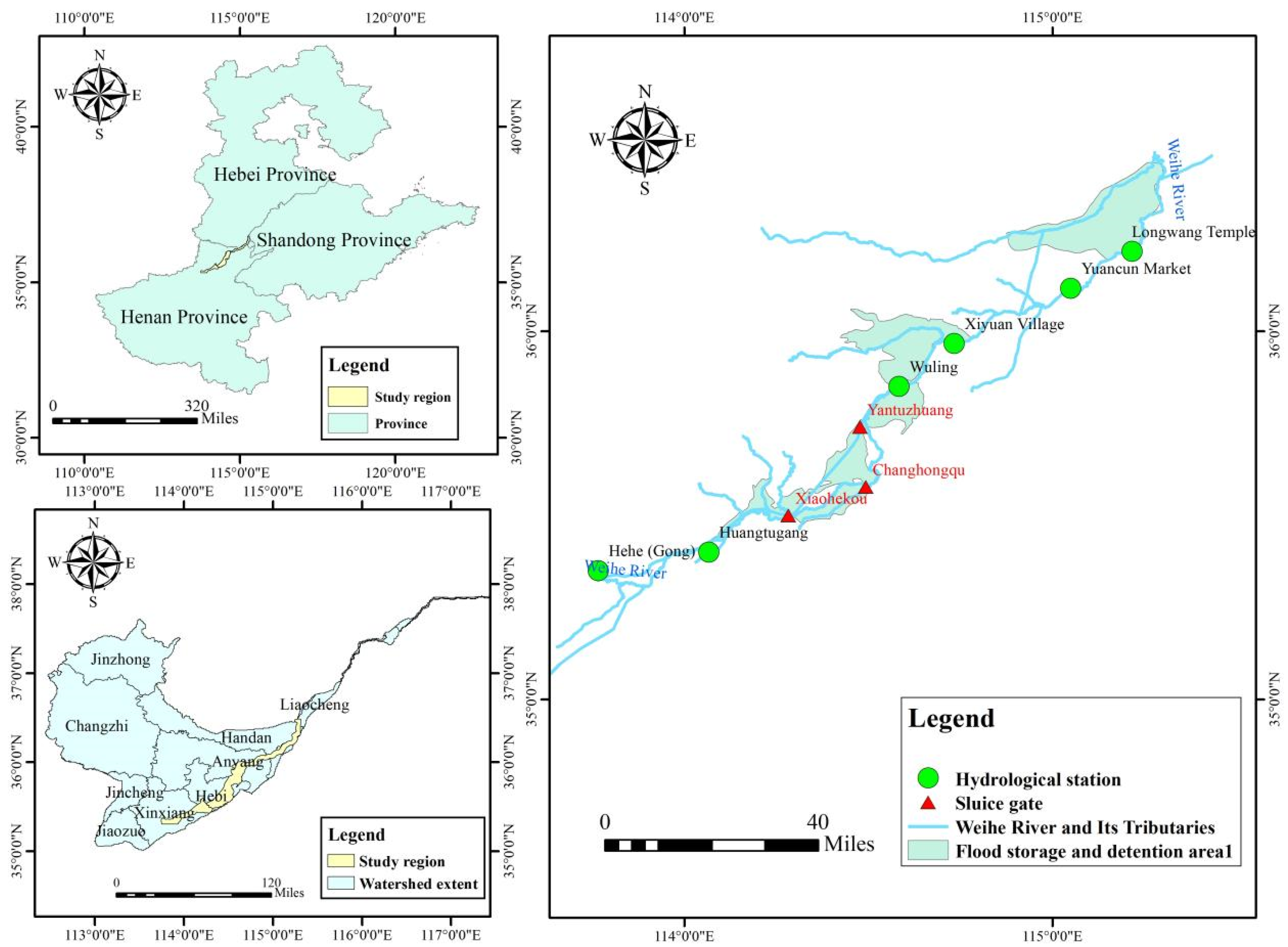
This study focuses on the Wei River Basin, located on the southern edge of the North China Plain. As a major tributary of the Haihe River system, the Wei River originates in Lingchuan County, Shanxi Province, flows from west to east through Henan and Shandong provinces, and finally discharges into the Zhangwei New River in Guantao County, Hebei Province. The main stream is approximately 400 km long, with a drainage area of 16,578 km².

Topographically, the basin exhibits a typical three-tier stepped distribution. The upper reaches belong to the residual Taihang Mountains, with elevations ranging from 200 to 1500 m, characterized by dramatic topographic relief and a gradually gentler terrain. The middle reaches consist of a piedmont alluvial–proluvial plain, with elevations between 50 and 200 m and a gradually gentle terrain. The lower reaches fully enter the North China Alluvial Plain, where the elevation drops below 50 m and the ground slope decreases to merely 0.1–0.5‰, forming a typical hanging river geomorphology. More than ten major tributaries, including the Qihe River, Tanghe River, and Anyang River, are distributed within the basin, collectively forming a dendritic drainage pattern.

Affected by the monsoon climate, the annual average precipitation in the basin ranges from 500 to 700 mm, but its spatial and temporal distribution is highly uneven. Approximately 70% of precipitation is concentrated from June to September, often occurring as short-duration, high-intensity rainstorms, with the maximum 24 h rainfall exceeding 400 mm [12,13].

The basin has experienced numerous catastrophic flood events throughout history. The extreme rainstorm event of 20 July 2021 caused severe disasters and economic losses in Zhengzhou and other adjacent areas, highlighting the vulnerability of the flood control system in the basin [14,15]. Given the large extent of the Wei River Basin, this study selects a critical river reach for flood control operation and flood routing simulation as the study area. The simulated river section takes Hehe (Gong) Sluice as the upstream control node and Luzhuang Pumping Station as the downstream outflow control node. The channel runs from southwest to northeast, successively traversing Xinxiang, Hebi, Anyang, and Puyang cities. Along the route, the main stream of the Wei River runs parallel to the Communist Canal, jointly undertaking flood discharge and water conveyance tasks for the basin, with a total length of approximately 118 km. The general situation of the study area is illustrated in Figure 1.

2.2. Available Information

This study utilized four types of open-source DEM data: the SRTM DEM (Shuttle Radar Topography Mission), jointly released by the National Aeronautics and Space Administration (NASA) and the National Geospatial-Intelligence Agency (NGA); the NASA DEM (National Aeronautics and Space Administration Digital Elevation Model), released by NASA; the AW3D30 DEM (Advanced Wide-Field-of-View 3D), released by the Japan Aerospace Exploration Agency (JAXA); and the ASTER DEM (Advanced Spaceborne Thermal Emission and Reflection Radiometer), jointly released by NASA and the Ministry of Economy, Trade and Industry (METI) of Japan. All of the above data were obtained from open-source websites. The download links and access dates for these DEM datasets are provided in the Supplementary Materials. Their specific basic information is shown in

Table 1. Basic information of each DEM data source.

Parameter	SRTM DEM	NASA	AW3D30	ASTER
Acquisition time	2000	2000	2006–2011	2000–2013
Release time	2015	2020	2019	2019
Coverage	60° N–56° S	60° N–56° S	80° N–80° S	83° N–83° S
Spatial Coordinate System	GCS_WGS_1984	GCS_WGS_1984	User_Defined_Transverse_Mercator	GCS_WGS_1984
Datum plane	D_WGS_ 1984	D_WGS_ 1984	D_WGS_ 1984	D_WGS_ 1984
Spatial resolution	30 m	30 m	30 m	30 m

.

ArcGIS10.8 was used to unify the coordinate system of the four open-source DEM datasets. The unified coordinate system was set to CGCS2000_3_Degree_GK_CM_114E.

2.3. Machine Learning Models

2.3.1. Random Forest

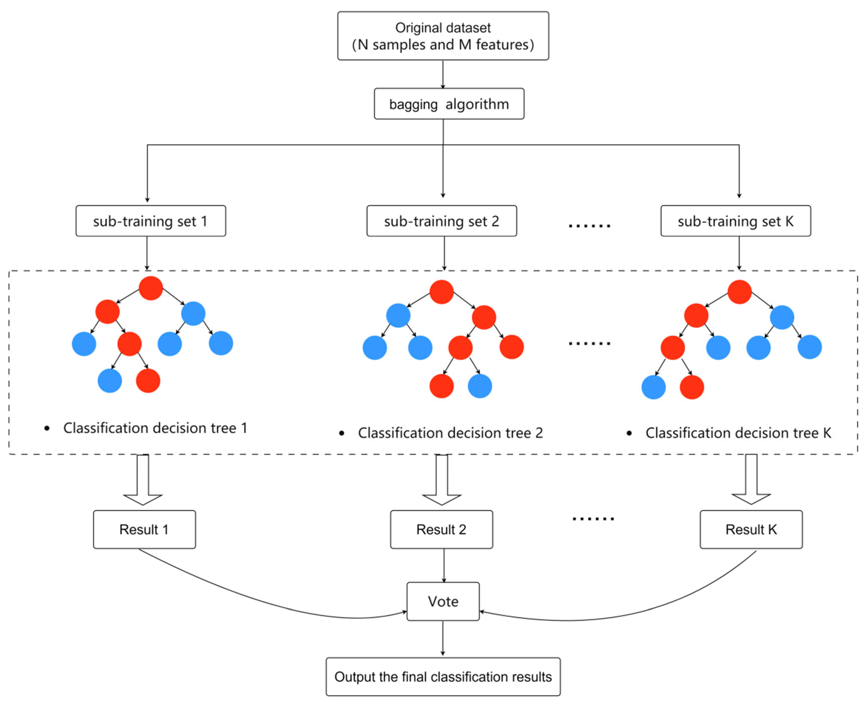
Random Forest (RF) is an ensemble learning algorithm based on the Bagging framework, proposed by Breiman in 2001 [16]. It consists of multiple decision trees that make predictions through “voting” or “average aggregation.” It offers advantages such as resistance to overfitting, strong robustness, and no need for strict assumptions regarding data distribution, making it suitable for nonlinear fitting and multi-source data modeling tasks under complex terrain conditions. The specific algorithm workflow is shown in Figure 2.

The core principles of Random Forests encompass two key randomization strategies. The first core principle is random sampling: using the Bootstrap sampling strategy, random samples are drawn with replacement from the original training set to generate independent training subsets for each decision tree. Samples not selected serve as out-of-bag (OOB) data, which can be used for model performance evaluation. This strategy ensures that each tree is trained on distinct samples, thereby reducing the risk of model overfitting. The second core principle is feature randomization. Using the random subspace method, during the splitting process at decision tree nodes, the algorithm does not select the optimal splitting feature from the entire feature set but instead randomly selects a subset of features for the splitting calculation. This method further reduces the correlation between decision trees, making the model more robust and suitable for modeling data with many features and high heterogeneity [17,18,19].

2.3.2. K-Means Clustering Algorithm

The K-Means clustering algorithm was proposed by J. B. MacQueen in 1967 [20]. Due to its computational simplicity and low linear time complexity, it is widely used in fields such as data mining and knowledge discovery. Generally, the objective of the K-Means clustering algorithm is to minimize the within-cluster sum of squared distances (WCSS), which is the sum of the squares of the distances from each point to the center of its assigned cluster. The formula for this is:

$$WCSS=\sum _{i=1}^K\sum _{p\in c_i}{\parallel p-{\mu }_i\parallel }^2$$

(1)

In the formula, K represents the number of clusters; $c_i$ denotes the set of points in the i-th cluster; $p$ represents a data point belonging to $c_i$; ${\mu }_i$ denotes the centroid of the i-th cluster; and ${\parallel p-{\mu }_i\parallel }^2$ denotes the squared Euclidean distance between the data point $p$ and the centroid ${\mu }_i$ of the cluster.

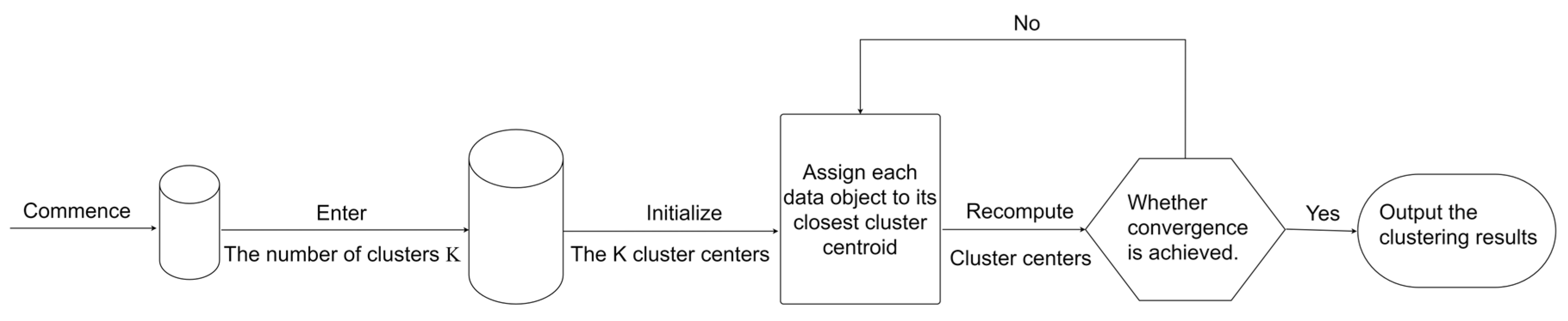
During the initialization phase of the K-Means algorithm, K data points are first selected as the initial cluster centers. The distance between each data point and these cluster centers is calculated, and the data point is assigned to the cluster with the shortest distance. It then recalculates the cluster centers for each cluster. Through an iterative process, it repeatedly calculates the distance from each data point to the cluster centers until the cluster centers no longer change or the criterion function converges to a specific value [21,22]. The specific process is shown in Figure 3.

2.3.3. Optuna Hyperparameter Optimization

Optuna is an efficient automated hyperparameter optimization framework based on the Bayesian optimization principle using the Tree-Structured Parzen Estimator (TPE). It iteratively samples and evaluates hyperparameter combinations and dynamically constructs a probabilistic surrogate model to guide subsequent search. Meanwhile, Optuna integrates a pruning strategy that terminates poorly performing parameter trials in advance, thereby concentrating computational resources on more promising parameter regions and significantly improving optimization efficiency and convergence speed [23,24,25].

In this study, Optuna is combined with a Random Forest fusion model to automatically search for the optimal hyperparameter combination within a predefined search space, enabling adaptive optimization of model structure and training parameters. This approach effectively addresses the challenges encountered in multi-source DEM fusion, including complex parameter tuning, low efficiency of manual trial-and-error, and unstable accuracy caused by multiple slope zones and multi-terrain feature inputs. As a result, the generalization ability and prediction accuracy of the fusion model are improved.

2.3.4. Building and Training Machine Learning Models

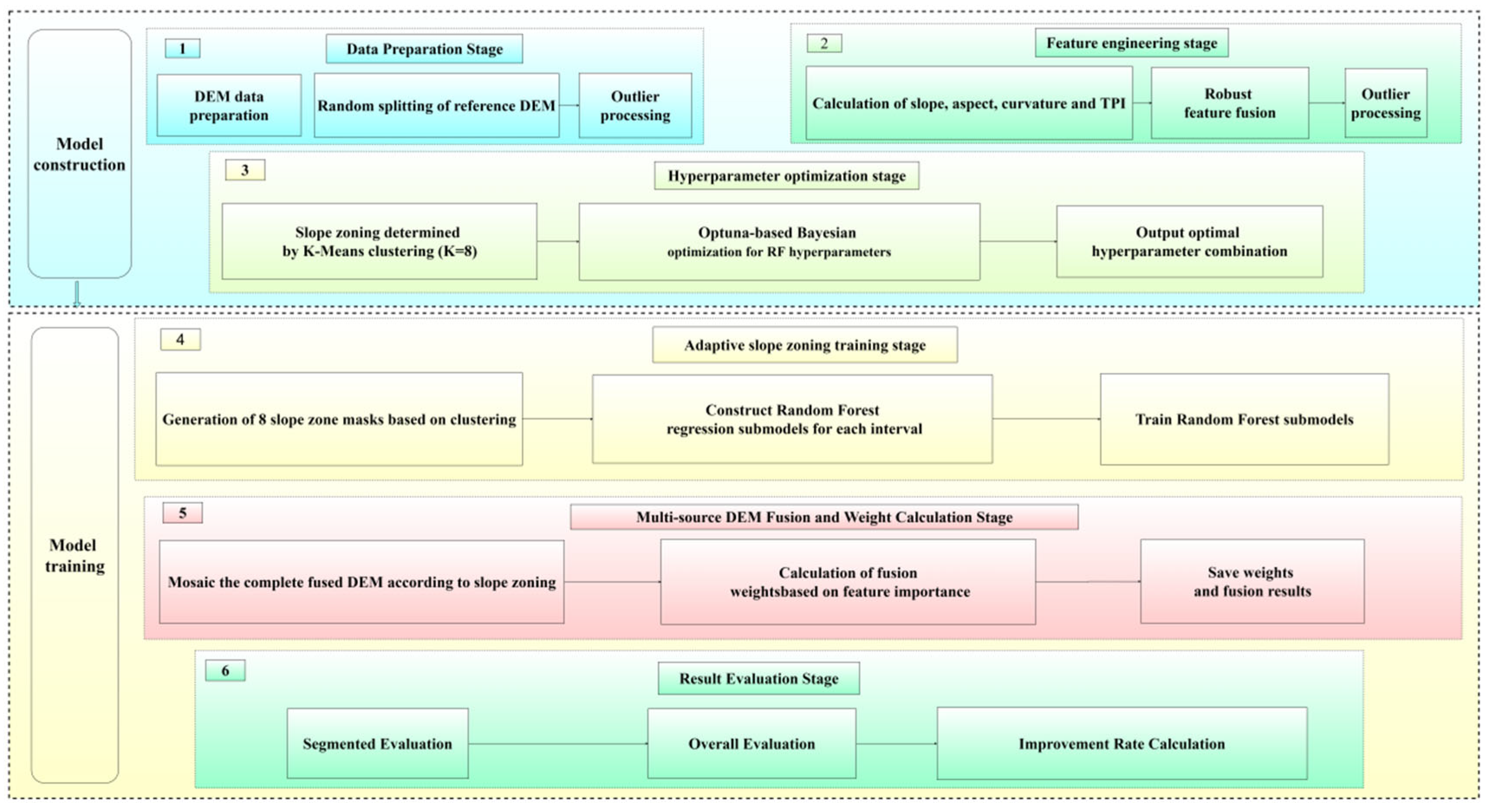
This model is a multi-feature fusion Random Forest regression model that integrates digital terrain analysis, cluster-based zoning, and ensemble learning techniques. It employs a hierarchical, modular hybrid architecture. The model not only effectively uncovers the nonlinear mapping relationship between multi-source DEM data and high-precision elevation data but also enhances its applicability and stability across different geographical environments through slope zoning. The specific model construction and training process are illustrated in Figure 4.

The specific model construction process consists of six stages: data preparation, feature engineering, Random Forest model establishment, parameter optimization, fusion weight calculation, and result output. The detailed procedures are described as follows:

(1)

Data preparation stage. The experimental data used in this study include one high-precision DEM of the Wei River and four low-precision DEMs, namely ASTER DEM, AW3D30 DEM, NASA DEM, and SRTM DEM. All DEMs are in txt format. It should be noted that this study currently focuses exclusively on the fusion of multi-source DEMs at a 30 m resolution. Furthermore, the adopted fusion method requires all source DEMs to share a uniform resolution and does not support the fusion of data with cross-resolutions. After the DEM data are collected, invalid value processing is performed on all DEM files by converting the value −9999 in the txt files to NaN, thereby facilitating subsequent statistical calculations and topographic feature processing.

(2)

Feature engineering stage. Based on digital terrain analysis (DTA) and the Sobel operator method [26,27], topographic features including slope, aspect, curvature and TPI are extracted. The corresponding calculation formulas are given as follows.

$$dx={\displaystyle \frac{(z_{i+1,j+1}+2z_{i,j+1}+z_{i-1,j+1})-(z_{i+1,j-1}+2z_{i,j-1}+z_{i-1,j-1})}{8\cdot cellsize}}$$

(2)

$$dy={\displaystyle \frac{(z_{i+1,j+1}+2z_{i+1,j}+z_{i+1,j-1})-(z_{i-1,j+1}+2z_{i-1,j}+z_{i-1,j-1})}{8\cdot cellsize}}$$

(3)

Slope calculation formula:

$$slope=arctan(\sqrt{({dx}^2+{dy}^2)})\times ({\displaystyle \frac{180}{\pi }})$$

(4)

Aspect calculation formula:

$$aspect=arctan2(-dy,dx)\times ({\displaystyle \frac{180}{\pi }})$$

(5)

$$aspect=aspect+360(ifaspect<0)$$

(6)

Curvature calculation formula:

$$dxx={\displaystyle \frac{d{x}_{i+1,j+1}+2d{x}_{i,j+1}+d{x}_{i - 1,j+1} - d{x}_{i+1,j - 1} - 2d{x}_{i,j - 1} - d{x}_{i - 1,j - 1}}{8\cdot cellsize}}$$

(7)

$$dyy={\displaystyle \frac{d{y}_{i+1,j+1}+2d{y}_{i+1,j}+d{y}_{i+1,j-1}-d{y}_{i-1,j+1}-2d{y}_{i-1,j}-d{y}_{i-1,j-1}}{8\cdot cellsize}}$$

(8)

$$\mathit{curvature}=-100 \times (\mathit{dxx}+\mathit{dyy})$$

(9)

Topographic Position Index (TPI) Formula:

mean_elev = mean elevation within the neighborhood (excluding the central cell)

TPI = elevation of central cell − mean_elev

In the equation, z represents the elevation value; $x$ represents the horizontal coordinate; $y$ represents the vertical coordinate; $cellsize$ represents the DEM grid size (in meters); $z_{i,j}$ is the elevation value (in meters) of the (i, j)-th cell in the DEM grid.

Finally, the fused topographic features of slope, aspect, curvature, and TPI are saved to the features cache folder, providing dataset support for subsequent model training.

(3)

Random Forest model construction stage. Considering that the DEM error distribution exhibits significant differences among various slope intervals, this study adopts the K-Means clustering method to realize adaptive slope zoning. To reduce bias caused by subjectively selecting the number of slope zones, a sensitivity analysis of slope zoning is carried out in this paper. Based on the K-Means algorithm, the slope dataset is clustered into 4, 6, 8, 12 and 100 categories respectively, so as to test the influence of different zoning schemes on the fusion accuracy. For each zoning scheme, the weighted Root Mean Square Error is adopted as the evaluation indicator; a smaller error value corresponds to better model performance.

$$WRMSE=\sqrt{{\displaystyle \frac{{\sum }_{i=1}^N{w}_i{(y_i-{\widehat{y}}_i)}^2}{{\sum }_{i=1}^N{w}_i}}}$$

(10)

Among them, the weight $w_i$ of the i-th sample is determined based on the number of pixels in the slope interval to which it belongs.

$$w_i={\displaystyle \frac{n_{bin\left(i\right)}}{{\sum }_{j=1}^K{n}_j}}$$

(11)

In the formula, N is the total number of valid pixels; $y_i$ is the true value of the i-th sample; ${\widehat{y}}_i$ is the predicted value of the i-th sample; $w_i$ is the weight assigned to the i-th sample; $n_{bin\left(i\right)}$ is the total number of pixels in the slope interval to which the i-th sample belongs; ${\sum }_{j=1}^K{n}_j$ is the total number of pixels across all K slope intervals; and K is the total number of slope intervals.

The comparison of the weighted RMSE of the fusion model under different numbers of slope intervals is shown in

Table 2. Comparison of weighted RMSE for different slope interval numbers.

Slope Intervals	4	6	8	12	100
Weighted RMSE	1.0714	1.0726	1.0690	1.0694	1.0758

(taking the Qimen-Xiyuancun section as an example). When the number of intervals was 4 and 6, the weighted RMSE values were 1.0714 and 1.0726, which are approximately 0.22% and 0.34% higher than those of the optimal interval scheme (K = 8), respectively. When the number of intervals increased to 8, the weighted RMSE reached its minimum value of 1.0690. When the number was further increased to 12, the weighted RMSE was 1.0694. When the number of intervals reached 100, the weighted RMSE rose to 1.0758. In conclusion, the weighted RMSE is minimized when K = 8. Therefore, this study ultimately determines to divide the slope into 8 intervals.

The slope thresholds are automatically calculated based on the K-Means clustering algorithm. First, the slope values of all valid pixels in the study area are extracted. Then, the K-Means algorithm (K = 8) is applied to cluster the slope data, yielding eight cluster centers. The midpoints between adjacent cluster centers serve as the partition boundaries, ultimately determining eight slope intervals. After the specific slope intervals are established, a Random Forest model is trained for each slope interval. Using the elevation values of the four low-precision DEMs and their topographic features (slope, aspect, curvature, TPI) as input features, and the elevation values of the high-precision DEM as the target variable, a feature matrix is constructed and regression models are trained.

(4)

Parameter optimization stage. The model achieves both random and Bayesian optimization of hyperparameters through the Optuna framework. In this stage, data is first cleaned and dimensionally aligned. NaN values in all features and the DEM are filtered out to ensure that the training data contains no outliers. To reduce the computational cost of the optimization process, this study performs slope-adaptive partitioning based on K-Means clustering, selects samples from the first slope interval as the optimization dataset, and extracts samples from this interval for hyperparameter search. With the minimization of the validation set Root Mean Square Error (RMSE) as the optimization objective, the optimal parameter combination is determined through multiple iterations, achieving precise tuning of the model’s hyperparameters. After the training of each interval model is completed, the models and partition boundary information are saved for use in the subsequent prediction stage.

(5)

Weight calculation stage for fusion results. After completing the model training for each slope interval, the feature importance of each Random Forest model is extracted. This metric reflects the contribution of each input feature to the model’s prediction results. The Random Forest model can output the contribution of each input feature to the prediction results, i.e., feature importance. The input features include the elevation values of four low-precision DEMs, slope, aspect, curvature, and the Topographic Position Index (TPI) under 3 × 3, 5 × 5, and 7 × 7 windows (TPI3, TPI5, TPI7). For the Random Forest model trained for each slope interval, a feature importance vector can be extracted.

$$I^{\left(m\right)}=[I_A^{\left(m\right)},I_B^{\left(m\right)},I_C^{\left(m\right)},I_D^{\left(m\right)},I_S^{\left(m\right)},I_{Aspect}^{\left(m\right)},I_{Curv}^{\left(m\right)},I_{TPI3}^{\left(m\right)},I_{TPI5}^{\left(m\right)},I_{TPI7}^{\left(m\right)}]$$

(12)

In the formula, $I_A^{\left(m\right)}, I_B^{\left(m\right)},{ I}_C^{\left(m\right)},{ I}_D^{\left(m\right)}$ are the feature importances of the four low-precision DEMs (ASTER, AW3D30, NASA, SRTM) within the m-th slope interval, respectively; $I_S^{\left(m\right)}$ is the feature importance of slope; $I_{\mathit{Aspect}}^{\left(m\right)}$ is the feature importance of aspect; $I_{\mathit{Curv}}^{\left(m\right)}$ is the feature importance of curvature; $I_{TPI3}^{\left(m\right)},{ I}_{TPI5}^{\left(m\right)},{ I}_{TPI7}^{\left(m\right)}$ are the feature importances of the Topographic Position Index (TPI) under 3 × 3, 5 × 5, and 7 × 7 windows.

By collecting the feature importance vectors from all eight slope interval models and calculating their mean, the average importance of each feature is obtained.

$${\overline{I}}_k={\displaystyle \frac{1}{8}}\sum _{m=1}^8{I}_k^{\left(m\right)}$$

(13)

Finally, the importance values of the four low-precision DEM features are extracted and normalized so that their sum equals 1, thereby obtaining the fusion weight for each low-precision DEM. The weight calculation formula is as follows:

$$w_k ={\displaystyle \frac{\overline{I_k}}{{\sum }_{k=1}^4\overline{I_k}}},j=1,2,3,4$$

(14)

In the formula, $\overline{I_k}$ represents the average feature importance of the k-th DEM across all slope intervals, and $w_k$ is its corresponding fusion weight.

The calculated weight results are saved in text file format and also summarized in an Excel spreadsheet to facilitate subsequent analysis and application.

(6)

Result output stage: The output results include the fused DEM file and the model evaluation file. For the fused DEM file, the prediction results of each slope interval model are first mosaicked according to their spatial positions to generate a complete fused high-precision DEM matrix. For valid pixels not covered during the training process, the overall prediction mean is used for filling. The fused DEM matrix is saved in text file format.

2.4. Flood Evolution Model

2.4.1. Model Principles

The two-dimensional hydrodynamic model, namely the Integrated Terrestrial Fluxes Model for Flood Forecasting (ITF-Flood), was independently developed by the China Institute of Water Resources and Hydropower Research (IWHR). This model adopts Graphics Processing Unit (GPU) parallel computing technology based on the Computer Unified Device Architecture (CUDA), which significantly improves the computational efficiency of numerical simulation. In the calculation process, the initialization of grid parameters and the configuration of boundary conditions are completed first. Subsequently, grid parameters and physical variables are transmitted to the video memory via the PCIe bus, and iterative calculations are then performed directly in GPU memory. Finally, the required physical variables are extracted for subsequent visualization processing and data analysis. With this architecture, the model supports kilometer-scale high-resolution simulation over the entire study area. Its computational speed is improved by two to three orders of magnitude compared with the traditional single-core CPU method.

The model discretizes the simulation domain into grid cells as computational units and simulates the hydrological and hydrodynamic processes within each grid cell, enabling high-resolution and high-efficiency simulation of basin flood routing processes. A simplified and efficient approach, namely the storage cell method, is incorporated into the model [28,29]. This method divides the study area into computational grid cells and solves the volume continuity equation for each cell. It can not only fully characterize the physical processes, but also effectively reduce computational consumption [30].

$${\displaystyle \frac{∆h}{∆t}}={\displaystyle \frac{∆V}{∆x∆y}}$$

(15)

In the formula, $∆h$ represents the Change in water depth of the cell, in meters; $∆\mathrm{t}$ represents the simulation time step, in seconds; $∆V$ represents the volume change in the cell within the time step; $∆x$ represents the dimension of the cell in the x-direction, in meters; $∆y$ represents the dimension of the cell in the y-direction, in meters.

The volume change ∆V of a cell is determined by the flux exchange with its four adjacent cells, and the flux between two cells can be calculated using the inertial form of Saint-Venant’s momentum equation:

$$q_{t+\Delta t}=\left(q_t-g{h}_{flow}\Delta t{S}_{surf}\right)/\left(1+{\displaystyle \frac{g{n}^2\left|q_t\right|\Delta t}{h_{flow}^{\frac{2}{3}}}}\right)$$

(16)

In the formula, $q_t$ is the flow rate per unit width at the cell boundary at time $t$, in m²/s; $\Delta t$ is the simulation time step, s; $S_{\mathit{surf}}$ is the water surface slope, dimensionless; $g$ is the acceleration due to gravity, m/s²; $n$ is the friction coefficient, s·m^−1/3; $h_{\mathit{flow}}$ is the critical flow depth, in m.

$S_{surf}$ is the water surface slope between adjacent cells, representing the ratio of the water surface elevation difference to the horizontal distance between the two cells:

$$S_{surf}={\displaystyle \frac{\Delta H}{\Delta L}}={\displaystyle \frac{(h_1+z_1)-(h_2+z_2)}{\Delta L}}$$

(17)

In the formula, $h_1$, $h_2$ are the water depths of two adjacent cells (m); $z_1$, $z_2$ are the ground elevations of two adjacent cells (m); $h_1+z_1$, $h_2+z_2$ are the water surface elevations of the two cells (m);$\Delta L$ is the horizontal distance between the centers of adjacent cells (m).

The critical flow depth between cells is defined as:

$$h_{\mathit{flow}}=\mathrm{m}\mathrm{a}\mathrm{x}(h_1+z_1,h_2+z_2)-\mathrm{m}\mathrm{a}\mathrm{x}(z_1,z_2)$$

(18)

In the formula, $h_1$, $h_2$ are the water depths at two adjacent computational cells (m); $z_1$, $z_2$ are the ground elevations of two adjacent cells (in meters, m).

To ensure numerical stability, the model adopts an adaptive time-stepping scheme based on the Courant–Friedrichs–Lewy (CFL) condition. The CFL number is maintained between 0.5 and 0.8. The time step is dynamically adjusted according to the grid size and flow velocity, and is calculated using the following formula:

$$\Delta t=CFL\times {\displaystyle \frac{\mathrm{m}\mathrm{i}\mathrm{n}(\Delta x,\Delta y)}{\sqrt{\mathrm{g}{h}_{\mathrm{m}\mathrm{a}\mathrm{x}}}}}$$

(19)

In the formula, $\Delta x$ and $\Delta y$ are the grid cell sizes (m); g is the gravitational acceleration (m/s²); $h_{\mathrm{m}\mathrm{a}\mathrm{x}}$ is the maximum water depth (m) across all grid cells at the current time step.

2.4.2. Model Building

The Wei River basin features a complex hydrological system with numerous flood storage and detention areas (FSDAs) and sluice structures. A unified model of the entire river section would suffer from excessive computational cost, low efficiency, and poor model stability. Therefore, this study divided the study area into segments based on the following two core principles:

(1)

Principle of FSDA distribution: The spatial distribution of the FSDAs—including Liangxiangpo, Liuweipo, Gongqu West, Changhongqu, Baishipo, Xiaotanpo, Rengupo, Guangrunpo, and Daming Floodplain—was used as key anchoring points. Specifically, the Qimen cross-section controls the inflow and outflow gates of both the Liuweipo and Liangxiangpo FSDAs and serves as the transition node between the upstream single-channel reach and the midstream FSDA cluster. Therefore, Qimen was selected as the boundary between the first and second reaches. Xiyuan Village is located between the core midstream FSDA cluster (Liangxiangpo, Liuweipo, Gongqu West, etc.) and the downstream Daming Floodplain. Using Xiyuan Village as a segmentation point allows the peak-attenuation effect of the midstream FSDA cluster to be simulated independently. Thus, Xiyuan Village was selected as the boundary between the second and third reaches.

(2)

Principle of key hydraulic structure control: The Hehe (Gong) Sluice serves as the main inlet for upstream inflow and the starting point of the main stream of the Wei River in the study area. With a complete record of measured discharge data, it was selected as the upstream boundary control node. Qimen is located downstream of the confluence of the Qihe River and the Communist Canal, surrounded by hydraulic structures such as the Xiaokoukou Control Gate. It is the core control works for the Liuweipo and Liangxiangpo FSDAs, and the area downstream of Qimen constitutes the midstream FSDA cluster. Selecting Qimen as a segmentation node enables precise simulation of the impact of upstream FSDA activation on the midstream reaches. The Luzhuang Pumping Station, as the downstream outflow control node of the Wei River basin with continuous outflow monitoring data, was selected as the downstream outflow boundary.

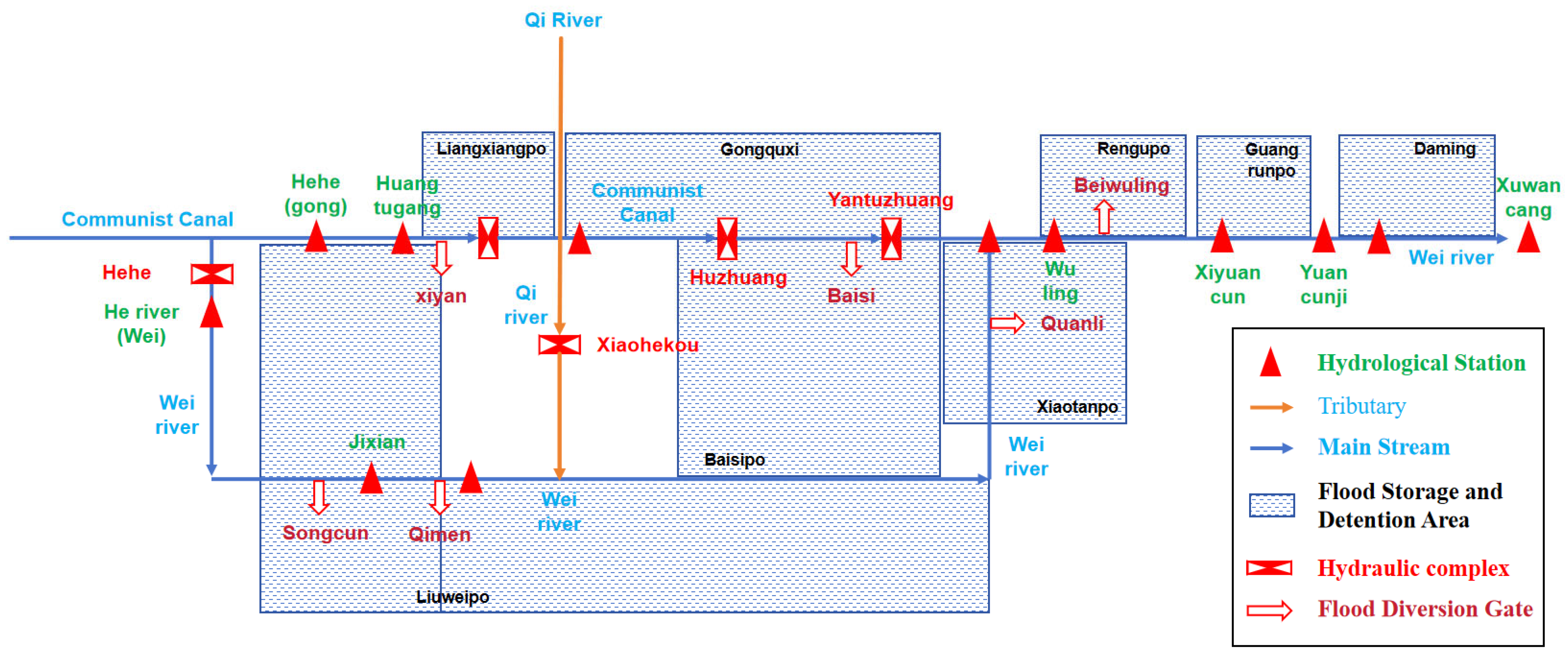
Based on the above principles and nodes, the study area was divided into three reaches: the Hehe–Qimen reach, the Qimen–Xiyuan Village reach, and the Xiyuan Village–Luzhuang Pumping Station reach. The topological simplification of the basin model is shown in Figure 5.

Using the ArcGIS10.8 software, the processing extent of each river reach was precisely constrained through the environment settings. The specific processing extents of each reach are shown in

Table 3. Processing range of each river section in ArcGIS10.8.

River Reach Name	Left (L) (m)	Top (T) (m)	Right (R) (m)	Bottom (B) (m)
Hehe (Gong) to Qimen	476,822.158437773	3,941,486.2664484	529,432.158437773	3,908,326.2664484
Qimen to Xiyuancun	523,022.158437773	3,986,816.2664484	563,687.158437773	3,927,251.2664484
Xiyuancun to Luzhuang Pumping Station	561,544.71008287	4,040,063.01399907	617,514.71008287	3,981,433.01399907

.

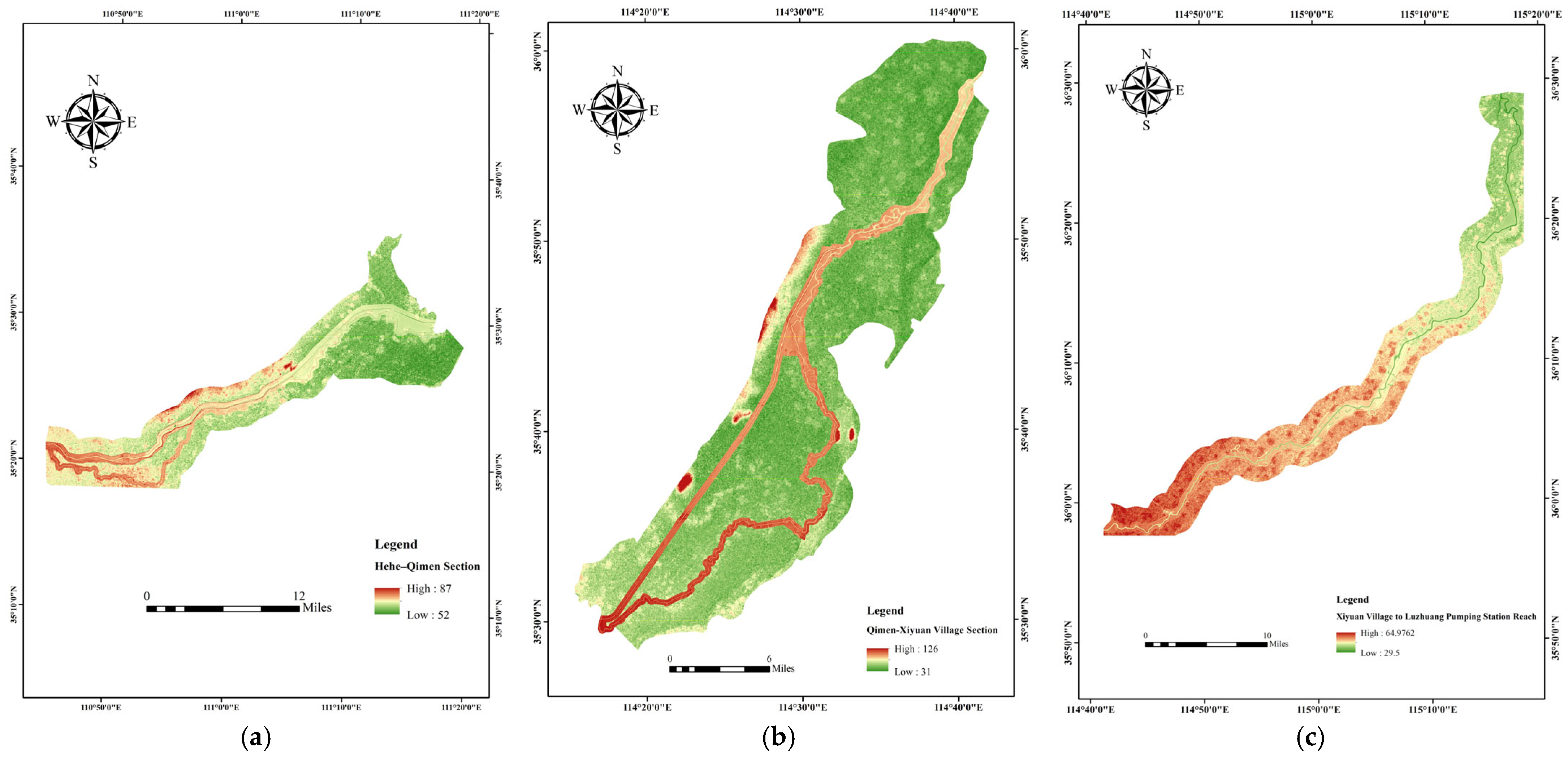
Mesh generation is a critical factor affecting the accuracy of two-dimensional hydrodynamic model results. The mesh generation in this study was based on DEM data of the Wei River and Gong Channel with a resolution of 2.5 m. The number of mesh elements in the three-segment two-dimensional hydrodynamic models was 17,445,476, 10,765,381, and 32,815,211, respectively. The construction of each model segment is shown in Figure 6.

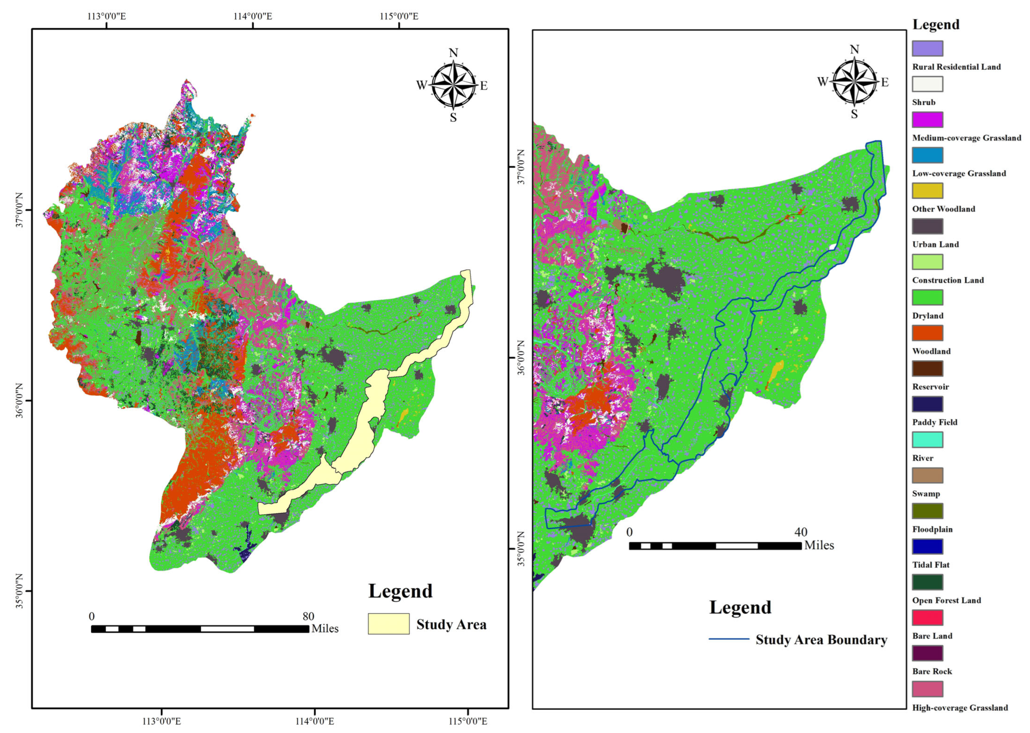
After the model construction was completed, the initial parameters were configured. The roughness coefficient is the most critical parameter affecting the model simulation accuracy, as it directly determines hydraulic characteristics such as flow resistance and riverbed morphology. The main land use types in the study area include dryland, rural residential land, and river channels, with dryland accounting for 79.74% of the total area (as shown in Figure 7). Referring to the recommended roughness coefficients for different land use types in the Hydraulic Calculation Manual and considering the actual underlying surface conditions of the study area, the roughness values for each land use type were assigned as follows: dryland 0.020, general vegetation 0.034, built-up area 0.030, bare land 0.020, and water bodies 0.025–0.035 [31]. For the river channel areas (the main stream of the Wei River and the Communist Canal), the roughness coefficient ranges from 0.02 to 0.05. Specifically, the roughness of the main channel of the Wei River is 0.025–0.035, while that of the floodplain is 0.035–0.050. As an artificial channel, the Communist Canal has a lower roughness of 0.020–0.030. Based on the above assignments, the overall roughness range of the study area is 0.02–0.05.

2.4.3. Model Calibration

To evaluate the accuracy and reliability of the model calibration, this study utilized the high-precision DEM and observed hydrological data of the “21 July” extreme basin-wide flood event in the Hai River Basin (from 02:00 on 21 July 2021 to 23:00 on 31 July 2021) to calibrate the model. A comparative analysis was conducted on the water level and discharge hydrographs at the two key hydrological stations of Hehe (Gong) Sluice and Wuling. The simulated discharge at Hehe (Gong) Sluice was 1329.26 m³/s, with a relative error of only 0.32% compared to the observed value; the peak occurrence time was 17:00 on 23 July, which coincided with the actual peak occurrence time. The simulated discharge at Wuling Station was 820.32 m³/s, with a relative error of 4.72% compared to the observed value; the peak occurrence time was 18:00 on 31 July, which also coincided with the actual peak occurrence time. The specific simulation results are shown in

Table 4. Comparison of simulated and observed cross-sectional results at gauged stations.

Key Cross-Section (Monitoring Station)		Maximum Water Level (m)	Relative Error	Peak Discharge (m3/s)	Relative Error	Peak Time	Error (h)
Hehe (Gong)	Actual value	76.77	1.84%	1325	0.32%	23 July at 17:00	0
	Simulated value	78.188		1329.26		23 July at 17:00
Wuling	Actual value	56.42	6.94%	861	4.72%	31 July at 18:00	0
	Simulated value	52.5		820.32		31 July at 18:00

.

Additionally, the Nash–Sutcliffe efficiency coefficient (NSE) was used as a model evaluation metric, with NSE = 0.5 set as the minimum value for assessing the reliability of the model calibration [32]. The NSE calculation method is as follows:

$$N_{SE}=1 - {\displaystyle \frac{{\sum }_{i=1}^N{(q_{i\_\mathrm{o}\mathrm{b}\mathrm{s}} - q_{i\_\mathrm{s}\mathrm{i}\mathrm{m}})}^2}{{\sum }_{i=1}^N{(q_{i\_\mathrm{o}\mathrm{b}\mathrm{s}} - {\overline{q}}_{\mathrm{o}\mathrm{b}\mathrm{s}})}^2}}$$

(20)

In the formula, N represents the number of measured flow data points; the subscript $i$ denotes the sequence number of the measured flow; $q_{i\_\mathrm{o}\mathrm{b}\mathrm{s}}$ represents the measured sequence; $q_{i\_\mathrm{s}\mathrm{i}\mathrm{m}}$ represents the simulated sequence; ${\overline{q}}_{\mathrm{o}\mathrm{b}\mathrm{s}}$ represents the mean of the observed values.

The results show that the Nash–Sutcliffe efficiency coefficient of the model for water level is 0.916 and that for discharge is 0.985, both greater than 0.9. This indicates that the simulation results are in good agreement with the observed data, and the simulation errors of key indicators such as the observed maximum water level are all within the 20% tolerance specified in the Standard for Hydrological Information and Forecasting [33]. The high goodness of fit demonstrates that the model accuracy meets the requirements.

3. Result

3.1. Analysis of Multi-Source DEM Fusion Results

3.1.1. Evaluation Criteria

To ensure an objective evaluation of the performance of the fused DEM, this study employs the following four metrics for quantitative assessment: Root Mean Square Error (RMSE), Mean Error (ME), Mean Absolute Error (MAE), and Standard Deviation of Error (SD) [34,35].

The formulas for calculating these metrics are as follows:

RMSE Formula:

$$RMSE=\sqrt{[{\displaystyle \frac{1}{m}}\times \sum {(y_{true,i}-y_{pred,i})}^2]}$$

(21)

ME Formula:

$$ME={\displaystyle \frac{1}{m}}\times \sum (y_{true,i} - y_{pred,i})$$

(22)

MAE Formula:

$$MAE ={\displaystyle \frac{1}{m}}\times \sum |y_{true,i} - y_{pred,i}|$$

(23)

SD Formula:

$$SD=\sqrt{[{\displaystyle \frac{1}{m}}\times \sum {(e_i-\overline{e})}^2]}$$

(24)

Specifically:

$$ei=y_{true,i} -{ y}_{pred,i}$$

(25)

$$\overline{e}={\displaystyle \frac{1}{m}}{\displaystyle \sum _{i=1}^m}{e}_i$$

(26)

In the formula, $m$ represents the number of valid pixels; $y_{true,i}$ represents the true value of the i-th pixel; $y_{pred,i}$ represents the predicted value of the i-th pixel.

3.1.2. Accuracy Analysis

This study analyzes the accuracy of the fusion results from three dimensions: weight distribution, slope zoning, and overall fusion performance.

For the Qimen–Xiyuan Village study section, analysis of the weight distribution results output by the fusion model reveals that the weight proportions of each individual DEM exhibit significant differences. Specifically, the SRTM DEM was assigned a weight of 0.4397, while the NASA DEM was assigned a weight of 0.3179. The combined weight of the SRTM DEM and NASA DEM reached 75.76%, a proportion that fully reflects the central role of these two data sources in the fusion model. Notably, the SRTM DEM’s weight accounts for nearly 50% of the total weight, further highlighting its dominant role in the multi-source data fusion process. Meanwhile, the AW3D30 DEM accounts for 17.5% of the total weight in the fusion model, while the ASTER DEM accounts for only 6.74%, making it the data source with the lowest weight among all sources. This weight distribution indirectly indicates that the characteristics of the ASTER DEM are less compatible with the feature requirements of the fusion model.

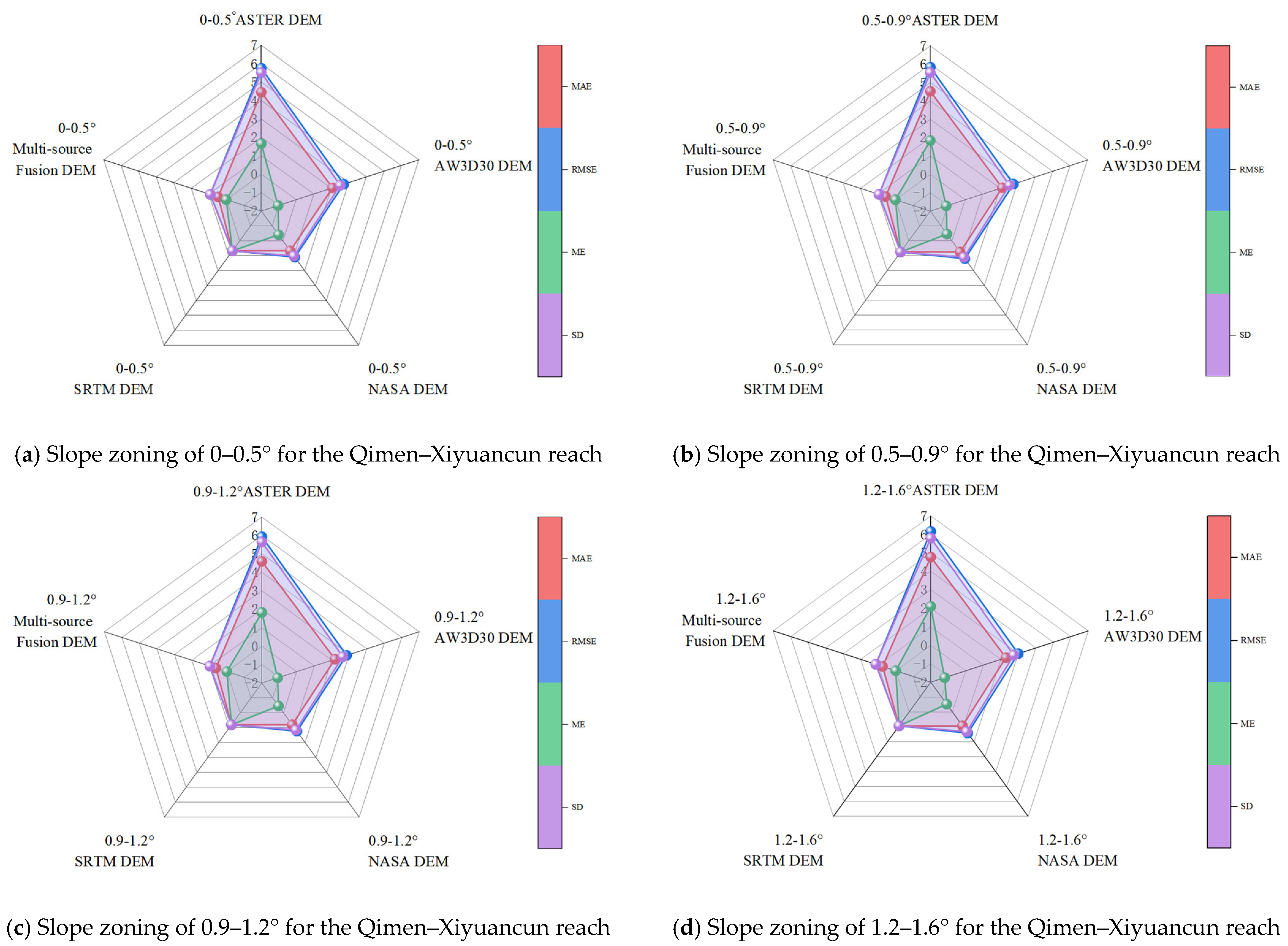
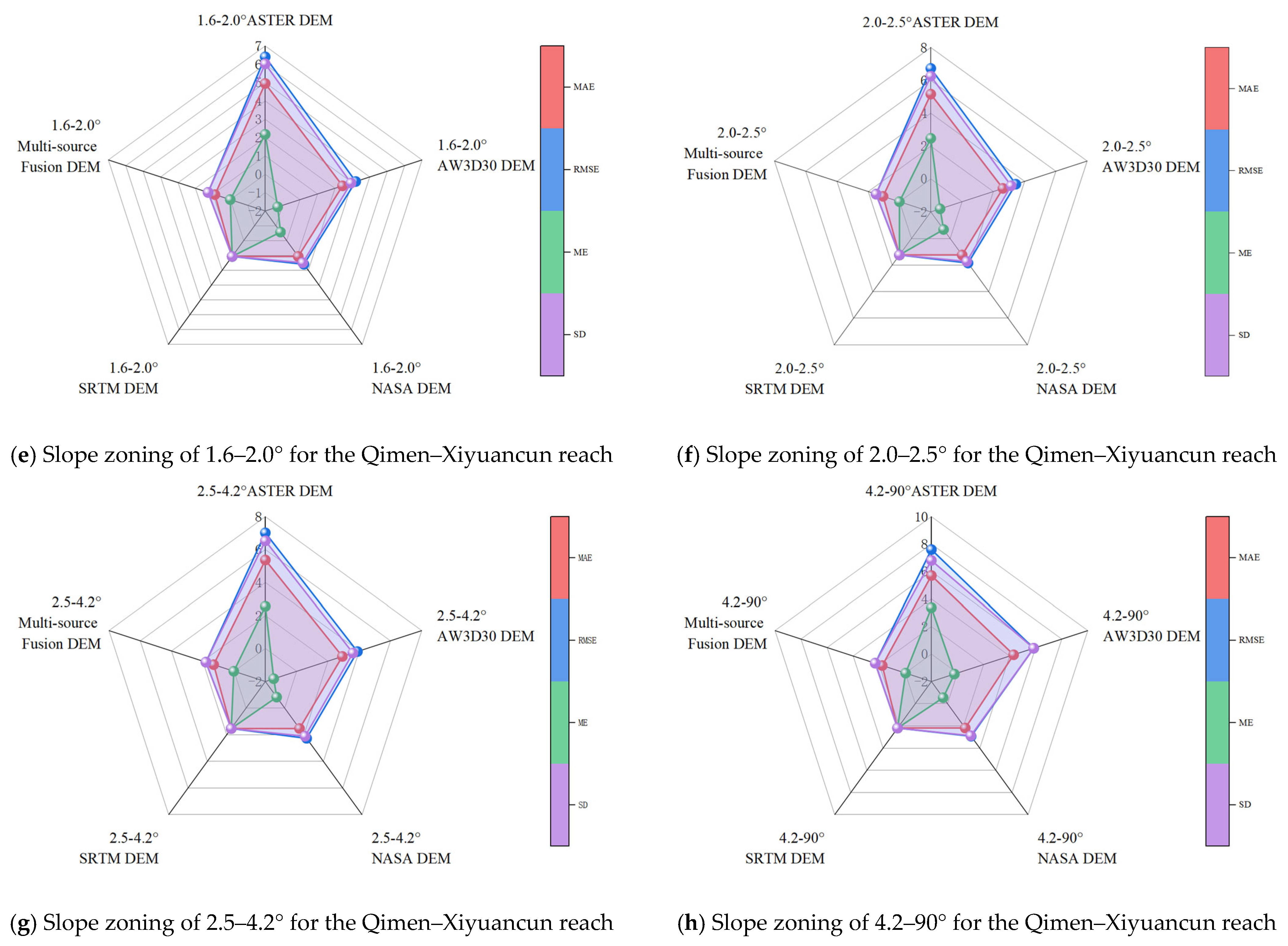
In terms of slope zoning, the model automatically divides the Qimen–Xiyuan Village section into eight consecutive slope intervals, with slope ranges of 0.0–0.5°, 0.5–0.9°, 0.9–1.2°, 1.2–1.6°, 1.6–2.0°, 2.0–2.5°, 2.5–4.2°, and 4.2–90.0° (see Figure 8 for detailed zoning results). Statistical analysis of the number of pixels in each slope interval revealed significant differences in pixel distribution across different slope intervals. Among these, the 0.9–1.2° slope interval had the highest number of pixels, reaching 536,789, accounting for a relatively high proportion of the total pixels in the study area; conversely, the 4.2–90.0° slope interval had the fewest pixels, with only 1995, indicating that the topography of this study area is dominated by moderate to low slopes.

A quantitative analysis of the accuracy metrics of the fused DEM within the 0.0–0.5° slope range reveals that the Mean Absolute Error (MAE) is 0.4687, the Root Mean Square Error (RMSE) is 0.9142, and the Mean Error (ME) is 0.0074. Crucially, the standard deviation (SD) of the error for the fused DEM in this range is exactly equal to the RMSE value. This characteristic indicates that the fusion model achieves excellent performance in the gently sloping plain areas, effectively integrating the advantages of multi-source data to produce high-precision elevation information.

As the slope range with the largest number of pixels (0.9–1.2°), the accuracy performance of its fused DEM is particularly noteworthy. The data show that the MAE of the fused DEM in this range is significantly lower than that of the other four single-source DEMs: 3.9653 lower than the ASTER DEM, 1.5540 lower than the AW3D30 DEM, and 0.1812 lower than both the NASA DEM and the SRTM DEM. This demonstrates the accuracy improvement achieved by the fusion model in the core slope range.

Within the 0.5–4.2° slope range, as slope values gradually increase, the accuracy of the fused DEM exhibits a steady decline. Specifically, the MAE metric rises from 0.5613 to 1.3052, while the RMSE metric increases from 0.9437 to 1.8007. Although there is a certain degree of accuracy degradation, the ME metric of the fused DEM remains close to 0 within this range, and the values of SD and RMSE remain consistent. This result indicates that the unbiased nature and error stability of the fused DEM do not change with increasing slope, and the model continues to demonstrate reliable performance in the moderate slope region.

For the high-slope range of 4.2–90.0°, accuracy analysis results show that the fused DEM has an MAE of 1.7651 and an RMSE of 2.3149. Comparing these accuracy metrics with those of the four original single-source DEMs (ASTER, AW3D30, NASA, and SRTM) reveals that the fused DEM’s metrics are closest to 0 across the board. It demonstrates the highest accuracy in the high-slope range, achieving a significant improvement in accuracy compared to the original single-source DEMs and effectively addressing the shortcomings of single-source DEM data in high-slope areas.

The above analysis indicates that the fusion model, with the SRTM DEM as its core input source, possesses strong terrain adaptability. It achieves optimal accuracy in plains and areas with gentle slopes, and while accuracy decreases steadily as slope steepness increases, the rate of decline is low, leaving bias and error stability unaffected. In steep slope areas, it significantly outperforms all single-source data.

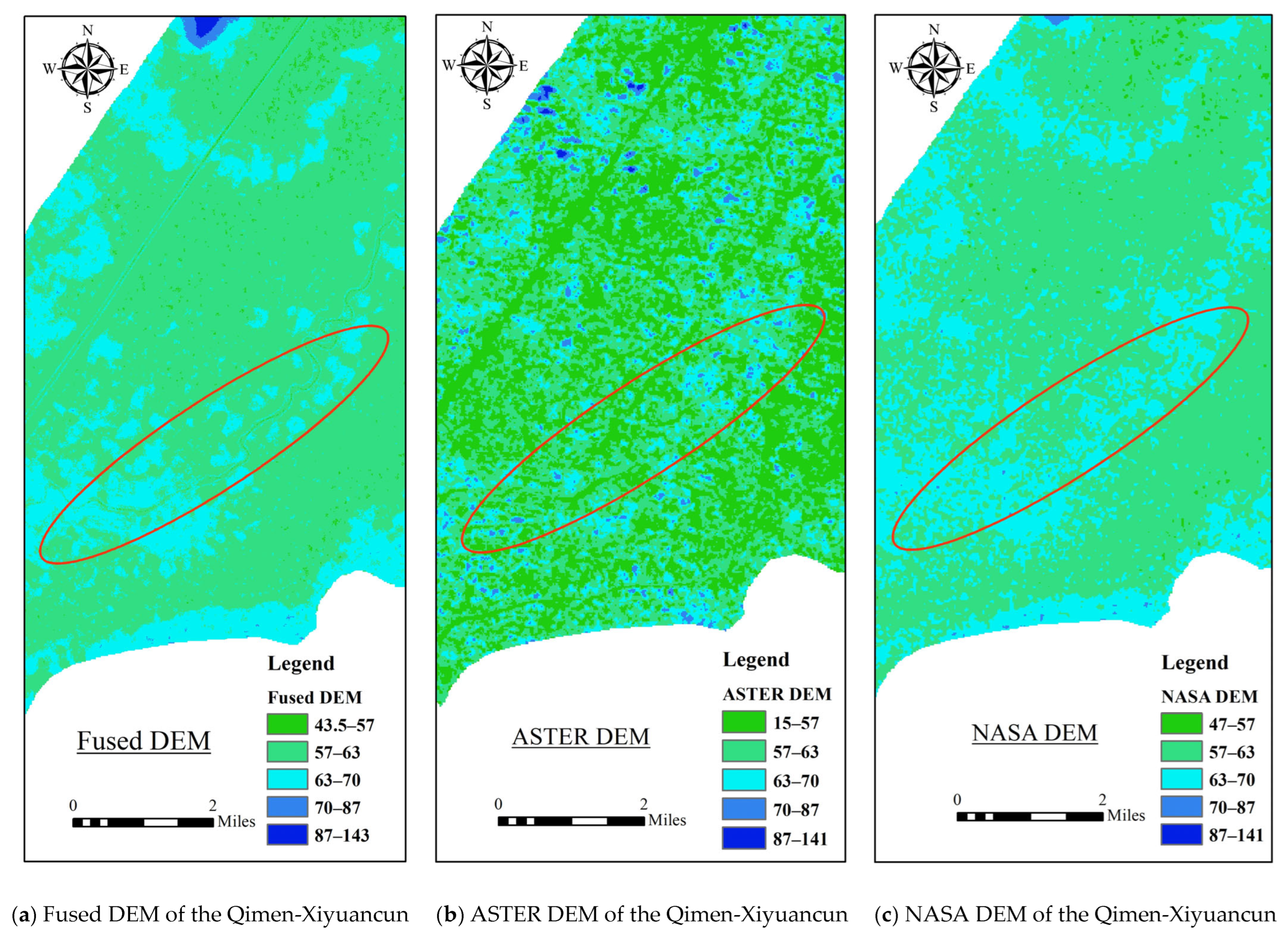
In terms of overall integration performance, the three-segment integrated DEM demonstrated excellent overall accuracy metrics. The specific parameters are as follows: Hehe (Gong)-Qimen section: MAE = 1.7218, RMSE = 2.3953, ME = −0.0085, SD = 2.3953. Qimen–Xiyuan Village section: MAE = 0.6880, RMSE = 1.0902, ME = 0.0027, SD = 1.0902. For the Xiyuan Village-Luzhuang section, MAE = 0.9855, RMSE = 1.4033, ME = 0.0082, SD = 1.4033. Notably, the absolute values of ME for the fused DEMs in all three sections approach 0, indicating that the fusion model has successfully eliminated any systematic bias that may have existed during the multi-source data fusion process. Additionally, the values of SD and RMSE are identical, a characteristic that collectively reflects the stable error distribution of the fused DEM. The model demonstrates exceptional predictive reliability and can provide high-precision, highly consistent elevation data support for the study area. As clearly shown in Figure 9, the river channel of the Wei River flowing through the flood detention area of the Changhong Channel exhibits a much clearer profile in the fused DEM compared to that of a single DEM.

A further quantitative assessment of the accuracy improvement of the fused model shows that the fused DEM achieves the most significant accuracy improvement compared to the ASTER DEM, with MAE improvements ranging from 58.13% to 85.32% and RMSE improvements ranging from 56% to 82.03%. This is followed by the AW3D30 DEM, with MAE improvements ranging from 54.72% to 70.55% and RMSE improvements ranging from 49.10% to 64.09%. For the NASA DEM, the improvements in MAE and RMSE are 21.32–63.50% and 20.36–52.99%, respectively. These results indicate that the accuracy improvements achieved by DEM fusion vary across different single-source DEMs, but overall, significant improvements are achieved.

Based on the above analysis, it can be concluded that the multi-source DEM fusion model developed in this study effectively extracts and utilizes complementary information among low-precision DEMs by employing an adaptive weighting mechanism for multi-source data. This approach reduces the inherent errors of low-precision data sources and demonstrates excellent fusion accuracy and performance. It can provide reliable elevation data for applications such as river terrain analysis and hydrological simulation.

3.2. Flood Process and Inundation Analysis Based on Different DEMs

Based on historical data from existing hydrological stations, this study simulated the flood that occurred from 19:00 on 20 July 2021 to 23:00 on 31 July 2021 (a total of 269 h). The model utilized SRTM DEM, NASA DEM, AW3D30 DEM, ASTER DEM, and a fused multi-source DEM as terrain data sources and compared the simulation results with the flood evolution process under high-precision DEMs. The Hehe (Gong), Huangtugang, and Xiyuan Village cross-sections were selected for flood process analysis.

3.2.1. Analysis of Flow Processes

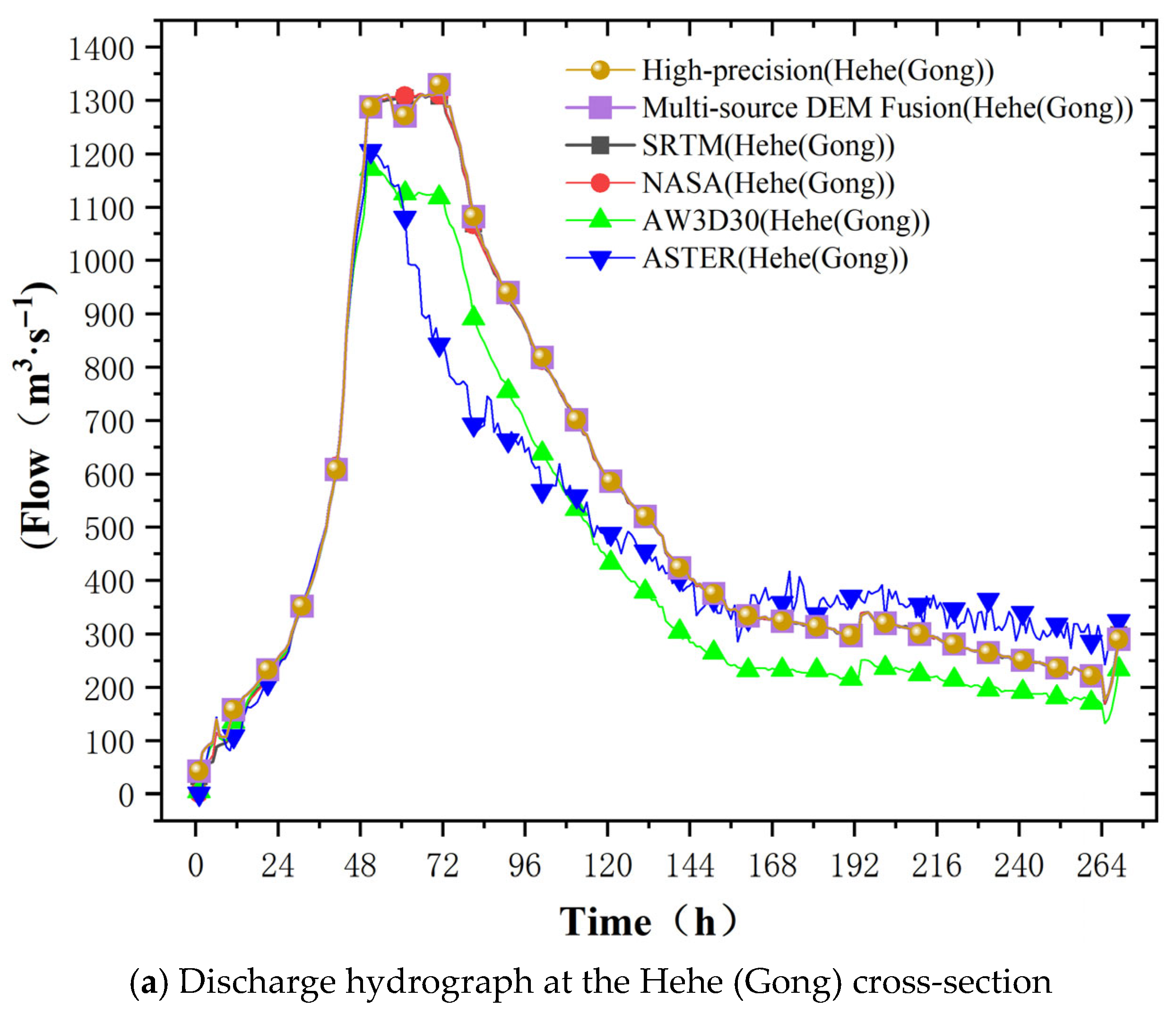
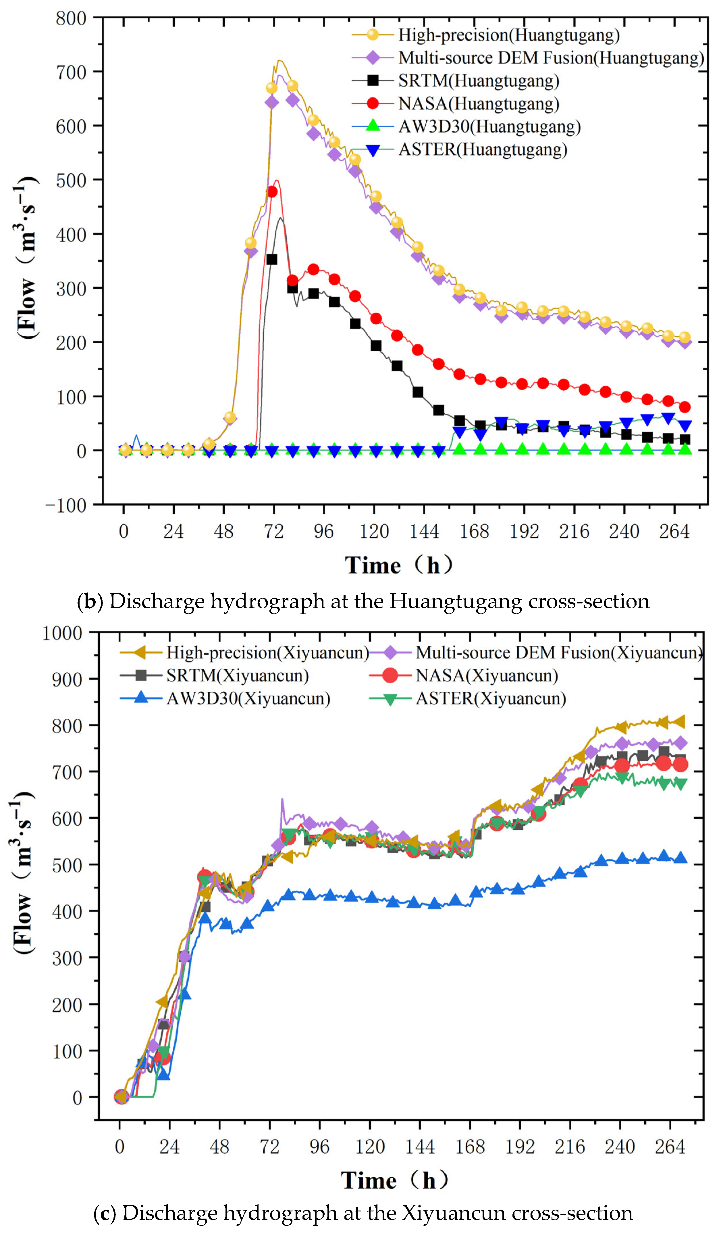
As shown in

Table 5. Peak flood data of representative cross-sections.

Section Name	Hydraulic Parameters	SRTM	NASA	ASTER	AW3D30	Fused DEM	High-Precision DEM
Hehe (Gong)	Flood peak date	23 July	23 July	23 July	22 July	23 July	23 July
	Flood peak time	12:00	11:00	1:00	21:00	11:00	17:00
	Maximum discharge (m3·s−1)	1310.79	1311.69	934.13	1171.62	1312.16	1329.26
	Relative error of discharge	0.014	0.013	0.297	0.119	0.013	0
Huang tugang	Flood peak date	23 July	23 July	21 July	21 July	23 July	23 July
	Flood peak time	21:00	19:00	1:00	1:00	18:00	20:00
	Maximum discharge (m3·s−1)	430.34	498.95	0.12	18.80	691.94	720.38
	Relative error of discharge	0.403	0.307	0.999	0.974	0.042	0
Xiyuancun	Flood peak date	31 July	31 July	30 July	31 July	31 July	31 July
	Flood peak time	14:00	3:00	12:00	15:00	7:00	13:00
	Maximum discharge (m3·s−1)	745.95	721.70	696.54	516.34	769.01	814.13
	Relative error of discharge	0.084	0.114	0.144	0.366	0.059	0

, at the Hehe (Gong) section, the simulated peak flood times and maximum discharge data from the fused DEM show only minor deviations from the high-precision DEM results. In terms of absolute error for maximum discharge, the fused DEM and SRTM DEM exhibit the best performance, with an error of only 0.013. The NASA DEM follows closely, with an error of 0.014. The AW3D30 DEM had an error of 0.119, performing well, while the ASTER DEM had the largest absolute error in maximum discharge, at 0.297. Regarding the time of peak flow occurrence, the fusion DEM data indicated a time of 11:00 on 23 July, differing by 6 h from the high-precision DEM. Compared to the AW3D30 DEM, which had an error of 20 h, and the ASTER DEM, which had an error of 16 h, the simulation results were significantly better.

At the Huangtugang section, the flood peak time and maximum discharge data from the fused DEM still maintain a relatively small discrepancy compared to the high-precision DEM. Compared to the single-source DEMs (SRTM, NASA, ASTER, and AW3D30), the relative error of maximum discharge decreased by 36%, 26.5%, 95.7%, and 93.2%, respectively. The maximum discharge values from AW3D30 and ASTER were significantly lower than those simulated by the high-precision DEM. These results indicate that the ASTER and AW3D30 DEMs may exhibit distortion in this region, which is consistent with their low weighting coefficients in the Random Forest simulation.

At the Xiyuancun section, the flood peak discharge calculated based on the fused DEM is 769.008 m³/s, while that derived from the high-precision DEM is 814.136 m³/s. The relative error of the flood peak discharge simulated by the fused DEM is 5.9%, which is superior to the simulation results of ASTER and AW3D30 DEMs. In terms of flood peak occurrence time, the peak time simulated by the fused DEM is 7:00 on 31 July, with a time difference of 6 h compared with 13:00 from the high-precision DEM. In contrast, the time differences in the NASA DEM and ASTER DEM relative to the high-precision DEM reach 10 h and 25 h, respectively. The above results indicate that the fused DEM outperforms all single-source DEMs in simulation performance.

In accordance with the requirements specified in the Standard for Hydrological Information and Hydrological Forecasting, the accuracy criteria for flood simulation are defined as follows: a flood event simulation is regarded as qualified if the relative error of the simulated flood peak discharge is ≤20%, and the error of the flood peak occurrence time shall not exceed 3 h. The results show that the relative error of flood peak discharge simulated by the fused DEM ranges from 1.3% to 5.9%, which fully meets the requirements of the forecasting standard. The error of peak occurrence time is 2–6 h, indicating that the flood peak arrival time in some simulation intervals fails to satisfy the specification. Nevertheless, the simulation results of the fused DEM are closest to those of the high-precision DEM, and obviously outperform the simulations based on single-source DEM data.

Regarding flow routing (Figure 10), to evaluate the fitting performance and prediction accuracy of the model for flood propagation, the coefficient of determination R² was selected as the goodness-of-fit evaluation metric. The closer R² is to 1, the stronger the explanatory power of the model and the better the fitting performance [36]. The specific formula for the goodness of fit is as follows:

$$R^2=1-{\displaystyle \frac{{\sum }_{i=1}^f{{(y}_i-\widehat{y})}^2}{{\sum }_{i=1}^f{(y_i-\overline{y})}^2}}$$

(27)

In the equation, f represents the number of measured values, $y_i$ represents the observed value, $\widehat{y}$ represents the model-fitted value, and $\overline{y}$ represents the mean of the observed values.

Based on the range of R² values, the data was divided into three intervals: 0–0.3, 0.3–0.7, and 0.7–1.0, corresponding to low, medium, and high levels of correlation, respectively. The R² values were analyzed using Origin’s nonlinear fitting tool. At the Hehe (Gong) section, the R² values for the multi-source DEM, SRTM, and NASA data were all 0.99, representing the most outstanding performance; these R² values were nearly 1, indicating a near-perfect fit. AW3D30 (0.98) and ASTER (0.90) were slightly lower but still exhibited strong correlation (R > 0.9). At the Huangtugang section, the fitting accuracy of NASA and the multi-source data fusion were 0.87 and 0.99, respectively, outperforming all other data sources, with SRTM (0.80) coming in second, while the R² value for AW3D30 was only 0.036 and that for ASTER was only 0.035. These R² values are nearly zero, indicating that both are extremely unreliable and show very poor performance in this region. At the Xiyuancun cross-section, the determination coefficient R² of SRTM is 0.97, that of NASA is 0.95, and the multi-source fused DEM reaches 0.98. All datasets achieve a high level of fitting performance, indicating that the fused DEM exhibits excellent reliability at this section. The R² values of ASTER and AW3D30 are 0.92 and 0.89, respectively, and their fitting accuracy is lower than that of the above three data sources.

In summary, multi-source fused data maintains a high level of fit across a variety of relevant scenarios. This is particularly evident at the Huangtugang cross-section, where the R² value is approximately 28.28 times higher than that of single data sources such as ASTER and AW3D30, significantly improving the fitting performance of single DEM data sources in low-correlation scenarios.

3.2.2. Analysis of Flooded Area and Flood Storage Capacity

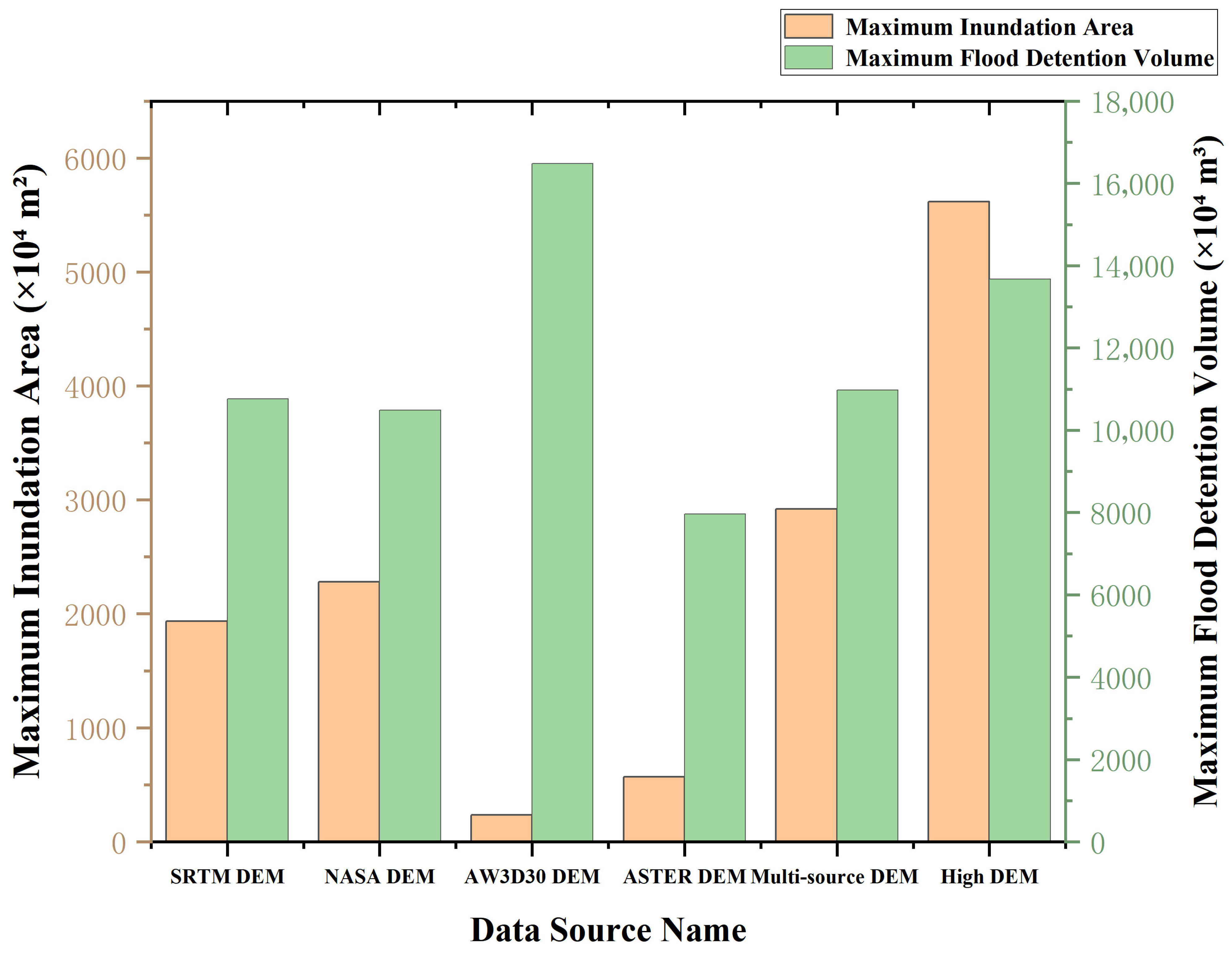
To systematically evaluate the suitability of different DEM data sources for simulating flood inundation in flood detention basins, this study selected the Gongqu (West) Flood Detention Basin as a representative case study. Based on two key metrics—maximum inundation area and maximum flood storage capacity—the study compared and analyzed the simulation results of the SRTM DEM, NASA DEM, AW3D30 DEM, ASTER DEM, multi-source fusion DEM, and high-resolution DEM. See Figure 11 for details.

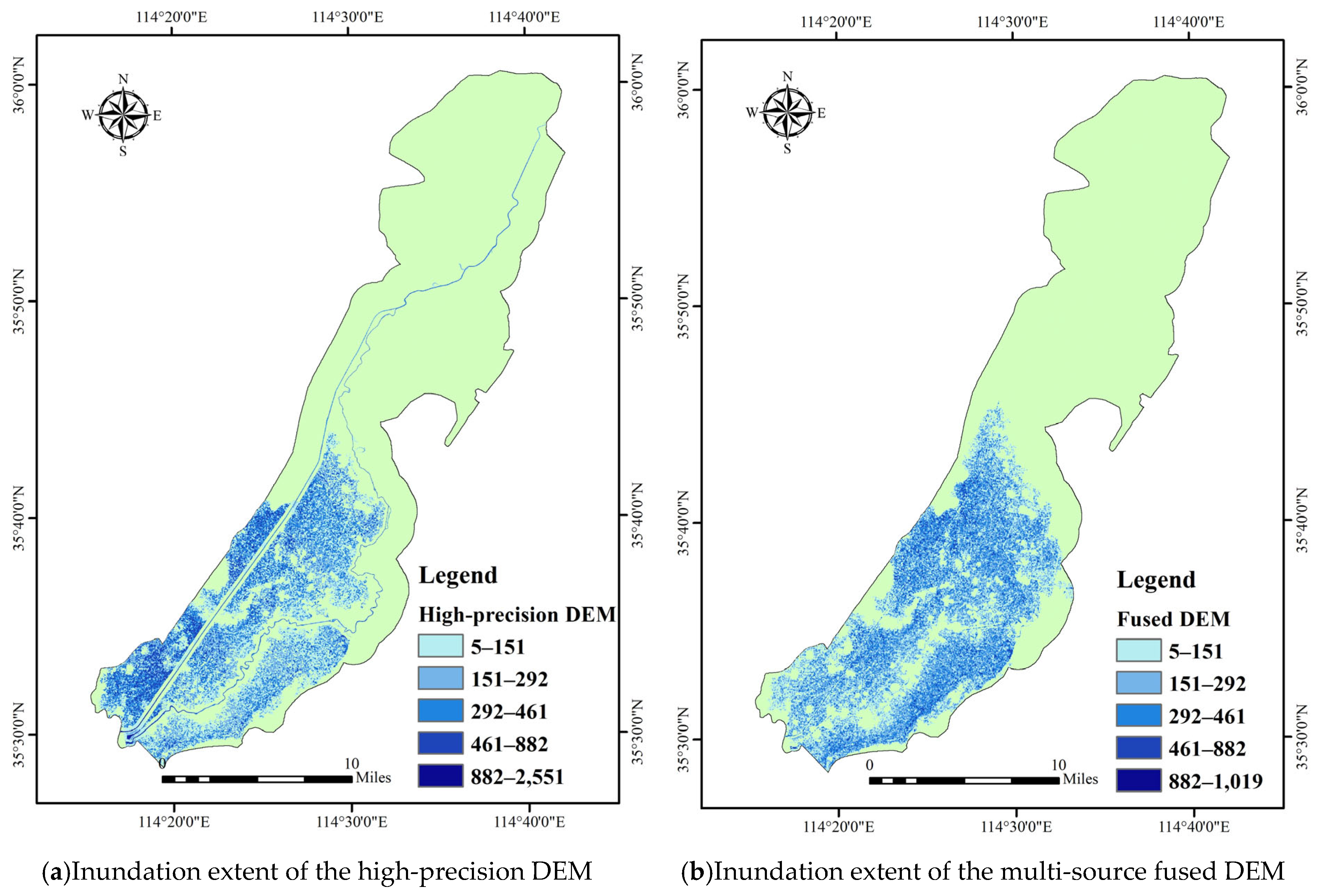
Regarding the simulation of the maximum inundation area, the maximum inundation area simulated by the high-precision DEM is 56.1557 million m². The relative errors of the SRTM DEM, NASA DEM, AW3D30 DEM, ASTER DEM, and the multi-source fused DEM compared to the high-precision DEM are 65.56%, 59.40%, 95.77%, 89.86%, and 37.64%, respectively. The simulated inundation areas from all data sources are significantly lower than those of the high-precision DEM, exhibiting a systematic underestimation characteristic. Among them, the simulation errors of the AW3D30 DEM and ASTER DEM are the most prominent, with relative errors both approaching 90%. First, ASTER DEM and AW3D30 are essentially Digital Surface Models, meaning their elevation values reflect the heights of vegetation canopies and building rooftops rather than the true bare-earth surface elevation. In areas such as the flood storage and detention area near the Huangdungang cross-section, characterized by flat terrain and dense human activity, this elevation error is particularly pronounced. Furthermore, the widespread presence of village buildings, shelterbelts, and crops around this cross-section leads ASTER DEM and AW3D30 to mistakenly incorporate the top heights of these features into the elevation data, creating a systematic positive bias. This results in significant deviations in the topographic representation of the flood storage and detention area, making it impossible to effectively reconstruct the actual inundation extent. The errors of the SRTM DEM and NASA DEM are similar, approximately 60%, indicating that their simulation accuracy remains relatively low. In contrast, the relative error of the multi-source fused DEM is only 37.64%, which is significantly lower than that of all individual DEM data sources. Moreover, as shown in Figure 12, the inundation results from the multi-source fused DEM are consistent with the actual inundation extent of the flood storage and detention area, demonstrating optimal performance in simulating the inundation extent.

In terms of maximum flood storage capacity, the high-precision DEM simulation for the Gongqu West Flood Storage Area yielded a maximum flood storage capacity of 136.746 million m³. The relative errors in maximum flood storage capacity for each DEM data source were as follows: SRTM DEM 21.30%, NASA DEM 23.35%, AW3D30 DEM 20.53%, ASTER DEM 41.80%, and multi-source fusion DEM 19.76%. The simulated flood storage capacities of all data sources were lower than those of the high-precision DEM, consistent with the tendency to underestimate inundation areas. The ASTER DEM had the highest error rate of 41.80% among all data sources, indicating the poorest simulation reliability; the SRTM DEM, NASA DEM, and AW3D30 DEM had similar error levels of approximately 20–23%, representing moderate simulation accuracy; the relative error of the multi-source fusion DEM was only 19.76%, representing the smallest flood storage capacity error among all data sources.

For the phenomenon that the fused DEM exhibits a relative error of 37.6% in the maximum inundation area and 19.76% in the maximum flood storage capacity compared with the high-resolution DEM, there are two main reasons. First, there is a spatial resolution limitation of the open-source DEM data. The basic data sources used for fusion are all open-source DEMs with a resolution of 30 m, including SRTM, NASA DEM, AW3D30 and ASTER. A 30 m resolution cannot capture micro-topographic features with a scale smaller than or equal to 15 m. Second, the fused DEM fails to retain artificial hydraulic structures such as dikes, bridges, revetments and road embankments. Taking dikes as an example, although they are distributed in a linear pattern, they are only reflected as an elevation rise of 1–2 pixels in the DEM. The fusion process is highly likely to cause distortion of dike elevation values and discontinuity of spatial topology, which changes the flood overflow conditions and further leads to a systematic underestimation of the inundation extent and flood storage capacity.

In summary, single-source DEMs exhibit obvious limitations in floodplain inundation simulation, with systematic underestimation errors in both inundation area and flood storage capacity, making them inadequate for high-precision flood simulation applications. In contrast, the multi-source fused DEM achieves much better performance. Its relative errors in maximum inundation area and flood storage capacity are remarkably lower than those of all single-source DEMs. Moreover, it can well reproduce the actual inundation scope of flood storage and detention areas, presenting the best overall simulation performance.

4. Discussion

This study proposes a multi-source DEM fusion method based on Random Forest, combined with K-Means slope zoning and Optuna hyperparameter optimization, which significantly improves the accuracy of terrain representation in the Wei River Basin and effectively supports the simulation of the “21 July” catastrophic flood event. Compared with existing DEM fusion methods (such as CNN and multiple linear regression), the innovations of this method lie in: first, the introduction of topographic factors (slope, aspect, curvature, TPI) as feature inputs, enabling the model to learn the mechanisms by which topographic heterogeneity influences elevation errors, rather than relying solely on numerical mapping of elevation values; second, the adoption of an adaptive slope zoning strategy, which avoids the problem of fitting distortion in topographically abrupt areas that plagues global models.

From the distribution of fusion weights, SRTM and NASA DEMs dominate the model, while the contribution of ASTER DEM is significantly lower. This difference not only reflects the varying topographic fidelity of different open-source DEMs in the Wei River Basin but also validates the rationality of the model’s feature importance learning.

At the level of slope zoning, the model achieves optimal fusion accuracy (MAE as low as 0.4687) in the 0–0.5°plain area. As the slope increases, accuracy declines steadily, but unbiasedness (ME ≈ 0) and error stability (SD ≈ RMSE) remain consistent throughout. This indicates that the proposed method possesses good topographic adaptability, making it particularly suitable for watershed areas where terrain transitions gradually from gentle to steep.

Although this method demonstrates excellent performance in the Wei River Basin, several limitations remain. First, the fusion input includes only four types of open-source DEMs, without incorporating high-precision point cloud data such as LiDAR or ICESat-2. Second, the generalizability of the method to extreme landform types such as karst and alpine canyon regions has not yet been validated. Third, the fused DEM does not incorporate hydrological key elements such as river engineering structures and levee elevations, which may affect the accuracy of local flood routing details.

Future research can be pursued in the following two directions. First, multi-source heterogeneous data (e.g., ICESat-2, UAV LiDAR) can be introduced to construct a hierarchical fusion strategy, optimizing training samples for different landform types. Second, a coupled model integrating multi-source DEM fusion and DEM correction can be developed, designing differentiated terrain correction strategies for the unique elevation anomaly characteristics of various man-made structures, such as bridges, levees, roads, culverts, and river barriers.

References

1. Zhang, W.; Liu, G.; Chiaka, J.C.; Yang, Z. Flood risk cascade analysis and vulnerability assessment of watershed based on Bayesian network. J. Hydrol. 2023, 626, 130144. [Google Scholar] [CrossRef]
2. Xu, K.; Wang, C.; Bin, L.; Shen, R.; Zhuang, Y. Climate change impact on the compound flood risk in a coastal city. J. Hydrol. 2023, 626, 130237. [Google Scholar] [CrossRef]
3. Ministry of Water Resources of the People’s Republic of China. Guiding Opinions and Implementation Plan on Promoting the Construction of Smart Water Conservancy. Water Conserv. Constr. Manag. 2022, 42, 5. [Google Scholar] [CrossRef]
4. Ministry of Water Resources of the People’s Republic of China. Guiding Opinions on Vigorously Promoting the Construction of Smart Water Conservancy; China Water Conservancy Press: Beijing, China, 2021. [Google Scholar]
5. Li, G.Y. Building digital twin watershed to promote high-quality development of water conservancy in the new stage. Water Resour. Dev. Manag. 2022, 8, 3–5. [Google Scholar] [CrossRef]
6. Li, J.Z.; Li, L.J.; Zhang, T.; Kang, Y.; Zhang, B.; Feng, P. Study on the influence of DEM data source and resolution on watershed flood simulation. J. Hydroelectr. Eng. 2023, 42, 26–40. [Google Scholar] [CrossRef]
7. Zhu, Y.; Burlando, P.; Tan, P.Y.; Gei, C.; Fatichi, S. Improving pluvial flood simulations with a multi-source digital elevation model super-resolution method. Nat. Hazards Earth Syst. Sci. 2025, 25, 2271–2291. [Google Scholar] [CrossRef]
8. Kulp, S.; Strauss, B.H. CoastalDEM v3.0: Improving Fully Global Coastal Elevation Predictions Through a Convolutional Neural Network and Multi-Source DEM Fusion; Climate Central Scientific Report; Climate Central: Princeton, NJ, USA, 2024. [Google Scholar]
9. Peramuna, P.; Neluwala, N.; Wijesundara, K.K.; Desilva, S.; Venkatesan, S.; Dissanayake, P.B.R. Enhancing 2D hydrodynamic flood model predictions in data-scarce regions through integration of multiple terrain datasets. J. Hydrol. 2025, 648, 132343. [Google Scholar] [CrossRef]
10. Zhang, R.; Pei, H. Analysis of multi-source DEM data fusion methods under different geomorphic conditions. China New Technol. New Prod. 2025, 18, 126–128. [Google Scholar] [CrossRef]
11. Liu, W.B. Research on improving terrain mapping accuracy by multi-source data fusion: A case study of typical geomorphic areas in Nancheng County, Jiangxi Province. North China Nat. Resour. 2025, 3, 90–93. [Google Scholar]
12. Zhang, X.X.; Yang, Y.C.; Ma, Q.; Xu, H.; Zheng, J.L.; Yang, B.; Yang, X.J.; Liu, C.J. Watershed flood review strategy driven by hydrological and hydrodynamic models. Chin. J. Appl. Basic Eng. Sci. 2026, 34, 76–88. [Google Scholar] [CrossRef]
13. Yin, P.F.; Wang, P.Y.; Zhao, W.L. Thoughts on suggestions for improving the flood control system in Wei River Basin. Haihe Water Resour. 2023, 4, 48–50. [Google Scholar]
14. Yang, W.Z.; Wang, P.Y.; Zhao, W.L. Comparative analysis of “63·8” and “21·7” rainstorm floods in Wei River Basin. Haihe Water Resour. 2023, 1, 66–69. [Google Scholar] [CrossRef]
15. Zhang, Y.; Zou, L.; Dou, M.; Wang, J.; Liu, Y. Water environmental risk assessment of different periods in Henan section of Wei River Basin. J. Agro-Environ. Sci. 2023, 42, 1778–1789. [Google Scholar] [CrossRef]
16. Breiman, L. Random Forests. Mach. Learn. 2001, 45, 5–32. [Google Scholar] [CrossRef]
17. Liu, B.; Mazumder, R. Randomization can reduce both bias and variance: A case study in Random Forests. J. Mach. Learn. Res. 2025, 26, 1–49. [Google Scholar] [CrossRef]
18. Mei, T.; Fan, Y.; Lv, J. Exogenous randomness empowering Random Forests. arXiv 2024, arXiv:2411.07554. [Google Scholar] [CrossRef]
19. Ma, Y.B.; Liu, S.Y.; Cao, D.P.; Feng, J.H.; Zhao, J.H. Application of Random Forest algorithm based on Bayesian optimization for reservoir prediction. Chin. J. Geophys. 2025, 68, 3247–3257. [Google Scholar] [CrossRef]
20. MacQueen, J. Some methods for classification and analysis of multivariate observations. In Proceedings of the 5th Berkeley Symposium on Mathematical Statistics and Probability, Berkeley, CA, USA, 21 June–18 July 1965; University of California Press: Oakland, CA, USA, 1967; Volume 1, pp. 281–297. [Google Scholar]
21. Zhang, L.N.; Zhang, X.R.; Ma, L.; Yu, H.L.; Song, X.Y. K-Means clustering algorithm optimized based on heuristic crossover strategy. J. Jilin Univ. (Sci. Ed.) 2025, 63, 1663–1672. [Google Scholar] [CrossRef]
22. Zhuang, Y.; Chen, X.; Yang, Y.; Wang, Z.; Liu, W. Statistically optimal K-Means clustering via nonnegative low-rank semidefinite programming. arXiv 2023, arXiv:2305.18436. [Google Scholar] [CrossRef]
23. Wang, K.Y.; Wang, Y.F.; Chen, X.; Liu, T.; Zhang, H. Remote sensing estimation of forest carbon storage in Jiangxi Province based on ensemble learning algorithm and Optuna optimization. Acta Ecol. Sin. 2025, 45, 685–700. [Google Scholar] [CrossRef]
24. Yang, F.; Xiao, F.; Shi, B.W.; Li, G.; Zhou, M. Deterioration trend assessment of hydropower units based on Optuna-CatBoost and CRITIC evaluation method. Water Resour. Power 2025, 43, 206–210. [Google Scholar] [CrossRef]
25. Neftissov, A.; Biloshchytskyi, A.; Kazambayev, I.; Kyzyrbekov, A.; Zhaparov, R. An Advanced Ensemble Machine Learning Framework for Estimating Long-Term Average Discharge at Hydrological Stations Using Global Metadata. Water 2025, 17, 2097. [Google Scholar] [CrossRef]
26. Wang, G.; Cao, J.; Sun, J.; Liu, Y.; Zhang, H. A multi-scale factor feature fusion modeling method for landslide susceptibility mapping. AIMS Geosci. 2026, 12, 335–359. [Google Scholar] [CrossRef]
27. Horn, B.K.P. Hill shading and the reflectance map. Proc. IEEE 1981, 69, 14–47. [Google Scholar] [CrossRef]
28. Guo, W.; Zhai, M.; Lei, X.; Huang, H.; Long, Y.; Li, S. Two-Dimensional Hydrodynamic Simulation of the Effect of Stormwater Inlet Blockage on Urban Waterlogging. Water 2024, 16, 2029. [Google Scholar] [CrossRef]
29. Bates, P.D.; de Roo, A.P.J. A simple raster-based model for flood inundation simulation. J. Hydrol. 2000, 236, 54–77. [Google Scholar] [CrossRef]
30. Dong, B.L.; Tan, C.; Xia, J.Q.; Wang, Y.; Li, J. Multi-GPU parallel acceleration of hydrodynamic model for rapid high-resolution urban flood simulation. Adv. Water Sci. 2026, 37, 199–208. [Google Scholar] [CrossRef]
31. Li, W. Hydraulic Calculation Handbook, 2nd ed.; China Water Power Press: Beijing, China, 2006. [Google Scholar]
32. Li, X.Y.; Hou, J.M.; Liu, Y.; Zhang, W.; Chen, L. Simulation of flood process in underground space under extreme rainstorm based on 1D-2D coupled hydrodynamic model. Chin. J. Hydrodyn. 2024, 39, 434–441. [Google Scholar] [CrossRef]
33. GB/T 22482-2008; Standard for Hydrological Information and Hydrological Forecasting. Standards Press of China: Beijing, China, 2008.
34. Zhao, S.; Cheng, W.; Jiang, J.; Wang, L.; Zhang, P. Error comparison among the DEM datasets made from ZY-3 satellite and the global open datasets. J. Geo-Inf. Sci. 2020, 22, 370–378. [Google Scholar] [CrossRef]
35. Meadows, M.; Jones, S.; Reinke, K. Vertical accuracy assessment of freely available global DEMs (FABDEM, Copernicus DEM, NASADEM, AW3D30 and SRTM) in flood-prone environments. Int. J. Digit. Earth 2024, 17, 2308734. [Google Scholar] [CrossRef]
36. Soliman, M.; Morsy, M.M.; Radwan, H.G. Generalized methodology for two-dimensional flood depth prediction using ML-based models. Hydrology 2025, 12, 223. [Google Scholar] [CrossRef]
Figure 1. Overview map of the study area.
Water 18 01201 g001
Figure 2. Random Forest algorithm flowchart.
Water 18 01201 g002
Figure 3. Flowchart of the K-Means clustering algorithm.
Water 18 01201 g003
Figure 4. Flowchart of machine learning model development and training.
Water 18 01201 g004
Figure 5. Topological schematic diagram of the Wei River Basin model.
Water 18 01201 g005
Figure 6. ITF-Flood model construction results. (a) Hehe-Qimen Section; (b) Qimen-Xiyuan Village Section; (c) Xiyuan Village to Luzhuang Pumping Station Reach.
Water 18 01201 g006
Figure 7. Land use map.
Water 18 01201 g007
Figure 8. Slope zoning maps of the Qimen-Xiyuan Village section under eight slope grades.
Water 18 01201 g008aWater 18 01201 g008b
Figure 9. Comparison of DEM results for the Qimen–Xiyuan Village section.
Water 18 01201 g009
Figure 10. Flow hydrographs for Hehe (Gong), Huangtugang and Xiyuancun sections.
Water 18 01201 g010aWater 18 01201 g010b
Figure 11. Flooding results for Gongqu (West).
Water 18 01201 g011
Figure 12. High-precision DEM versus fused DEM inundation area comparison map for the Qimen-Xiyuan Village section.
Water 18 01201 g012