Influence of DEM Spatial Resolution on the Accuracy and Computational Efficiency of HEC-RAS 1D and 2D Flood Inundation Modelling: A Case Study of the Cimanceuri Basin, Indonesia

Abstract

Digital Elevation Model (DEM) resolution plays a critical role in hydraulic flood modelling by influencing inundation accuracy, spatial precision and computational efficiency. However, limited studies have simultaneously evaluated both inundation accuracy and computational performance across multiple DEM resolutions in event-based urban flood modelling. This study aims to evaluate the impact of DEM spatial resolution on the performance of HEC-RAS 1D and 2D models in simulating an event-based urban flood that occurred on 3 March 2025. A 1 m LiDAR-derived DEM was resampled to 2 m, 5 m, 8 m, 10 m, 20 m, 25 m, and 30 m resolutions to assess the effects of terrain generalization on hydraulic response. Simulated inundation extents were validated against observed flood areas derived from aerial imagery, and computation time was recorded for each scenario. Results reveal a clear trade-off between spatial accuracy and computational demand. In the 1D simulations, deviation from observed inundation increased from 0.76 ha at 1 m to 2.50 ha at 30 m, while computation time remained relatively stable. The 2D simulations were more sensitive to DEM resolution, with deviation increasing from 0.33 ha to 3.12 ha and longer runtimes at finer resolutions. Among the evaluated scenarios, the 10 m DEM provided the most balanced performance in both 1D and 2D models. For rapid assessment and operational flood management, where computational efficiency and timely decision-making are critical, a 1D modelling approach combined with a 10 × 10 m DEM is recommended as a practical and efficient solution.

1. Introduction

Flooding is one of the most hazardous natural disasters, significantly affecting human life and the sustainability of infrastructure, particularly in developing countries [1]. Floods are caused by a combination of natural processes and human activities [2]. Accurate flood inundation mapping is essential for effective flood risk management, urban planning, and early warning systems, enabling stakeholders to plan mitigation strategies and issue timely alerts to minimize potential impacts [3,4]. Hydraulic models are widely used to simulate flood dynamics and delineate inundation extents under various hydrological scenarios [5,6].

Hydrodynamic simulations are widely used to assess flood inundation extents and support non-structural flood management strategies. However, decision-makers and researchers often have varying levels of experience when selecting appropriate hydrodynamic modeling approaches [7]. Many studies have applied the Hydrologic Engineering Center—Hydrologic Modelling System (HEC-HMS) in combination with the Hydrologic Engineering Center—River Analysis System (HEC-RAS) to improve the understanding and prediction of flood events [8,9,10,11]. In flood modelling, HEC-RAS can be applied using different hydraulic modelling approaches, including one-dimensional (1D) and two-dimensional (2D) simulations. Among these approaches, 1D hydraulic models such as HEC-RAS remain widely used due to their lower computational requirements and relatively simple implementation. Although 2D models can represent flood behavior with greater spatial detail, their high computational cost often makes them less practical for operational or event-based flood analysis [5].

Digital Elevation Models (DEMs) are advanced tools for terrain analysis, as they provide more detailed surface information compared to other types of satellite imagery [12]. DEM data is the fundamental input for 2D hydraulic modelling, as they directly influence channel geometry, floodplain representation, and water surface profiles [13]. Previous studies have demonstrated that DEM resolution can significantly affect flood simulation results, including inundation extent and water level estimates [14]. However, increasing DEM resolution does not always lead to proportional improvements in modelling accuracy, and an optimal resolution threshold may exist depending on watershed characteristics [15].

Advances in remote sensing technology, particularly Light Detection and Ranging (LiDAR), have enabled the generation of high-resolution Digital Elevation Models (DEMs) that significantly improve terrain representation for hydraulic modelling. High-resolution DEMs can capture detailed topographic features such as riverbanks, floodplains, and urban structures, which are essential for accurately simulating flood dynamics. However, increasing DEM resolution also leads to larger data volumes and higher computational demands, which may not always result in proportional improvements in modelling accuracy [16]. Although several studies have investigated the influence of DEM resolution on flood modelling performance, determining the most appropriate DEM resolution remains challenging [15,17]. Comprehensive assessments that simultaneously evaluate inundation accuracy and computational efficiency across multiple DEM resolutions are still relatively limited, especially in event-based urban flood modelling applications [2,8,18,19]. This issue is particularly relevant in rapidly developing tropical regions, where timely flood simulation results are essential to support effective flood risk management and decision-making.

One-dimensional (1D) hydraulic models are widely used for river flow analysis due to their computational efficiency and ability to represent longitudinal water surface profiles along the channel [20,21]. In this approach, flow is primarily simulated along predefined cross-sections, which simplifies lateral flow processes across the floodplain. Although this framework is computationally efficient, it may limit the representation of complex floodplain dynamics, particularly in urban environments where water spreads in multiple directions. In contrast, two-dimensional (2D) hydraulic models solve the shallow water equations over a computational grid, enabling flow simulation in both longitudinal and lateral directions and providing a more detailed representation of flood inundation processes [20,21].

Because these two modelling approaches differ in their representation of floodplain flow and computational demand, comparing their performance is important for understanding how terrain representation influences flood simulation results. In particular, the spatial resolution of DEMs plays a crucial role in hydraulic modelling because terrain data directly control flow pathways, inundation extent, and computational requirements.

This study contributes to the existing literature through three key aspects: (1) evaluating the influence of DEM spatial resolution within an event-based urban flood context, (2) integrating and comparing 1D and 2D hydraulic modelling approaches under consistent hydrological conditions, and (3) jointly assessing flood inundation accuracy and computational efficiency within a single modelling framework. These combined aspects provide a more comprehensive understanding of model performance compared to previous studies, which typically address these factors separately.

Table 1. Comparison with previous studies.

Study	DEM Resolution Analysis	1D/2D Comparison	Computational Efficiency	Event-Based Analysis	Key Contribution
Zhu & Chen [15]	✔	✖	✖	✖	DEM impact
Amellah et al. [22]	✔	✔ (2D focus)	✖	✖	2D flood mapping
Apel et al. [23]	✖	✔ (2D focus)	✔	✔	Urban Flood modelling
Cook & Merwade [24]	✔	✖	✖	✖	DEM & geometry influence
Sanders [25]	✔	✖	✔	✖	DEM vs. computational cost
This study	✔	✔	✔	✔	Integrated evaluation

highlights that previous studies generally examine DEM resolution, modelling approaches, or computational efficiency separately. In contrast, this study provides a comprehensive evaluation by combining these aspects within a single modelling framework, thereby offering a more holistic understanding of flood modelling performance.

Unlike previous studies that primarily focus on either model accuracy or DEM resolution effects in isolation, this study presents a comprehensive assessment of the influence of DEM spatial resolution on both flood inundation accuracy and computational efficiency using an integrated HEC-HMS–HEC-RAS modelling framework. In addition, this research uniquely evaluates the performance of both 1D and 2D hydraulic models under consistent hydrological conditions within the Cimanceuri River basin. The use of LiDAR-derived DEM resampled into multiple resolutions, combined with quantitative evaluation using inundation area deviation (ΔA), provides a more systematic and location-specific understanding of model sensitivity to terrain representation. This approach offers practical insights for optimizing model configuration in data-rich yet computationally constrained environments. Therefore, the objectives of this study are to:

  (i)

Evaluate the influence of DEM spatial resolution on the performance of HEC-RAS 1D and 2D flood inundation models;

 (ii)

Compare flood inundation accuracy and computational efficiency across multiple DEM resolutions; and

(iii)

Identify an optimal DEM resolution that provides a practical balance between modelling accuracy and computational demand.

The remainder of this manuscript is organized as follows. Section 2 describes the study area, datasets, and modelling methodology. Section 3 presents the results and discussion of hydrological and hydraulic simulations. Section 4 summarizes the main conclusions and recommendations for future research.

2. Materials and Methods

2.1. Study Area

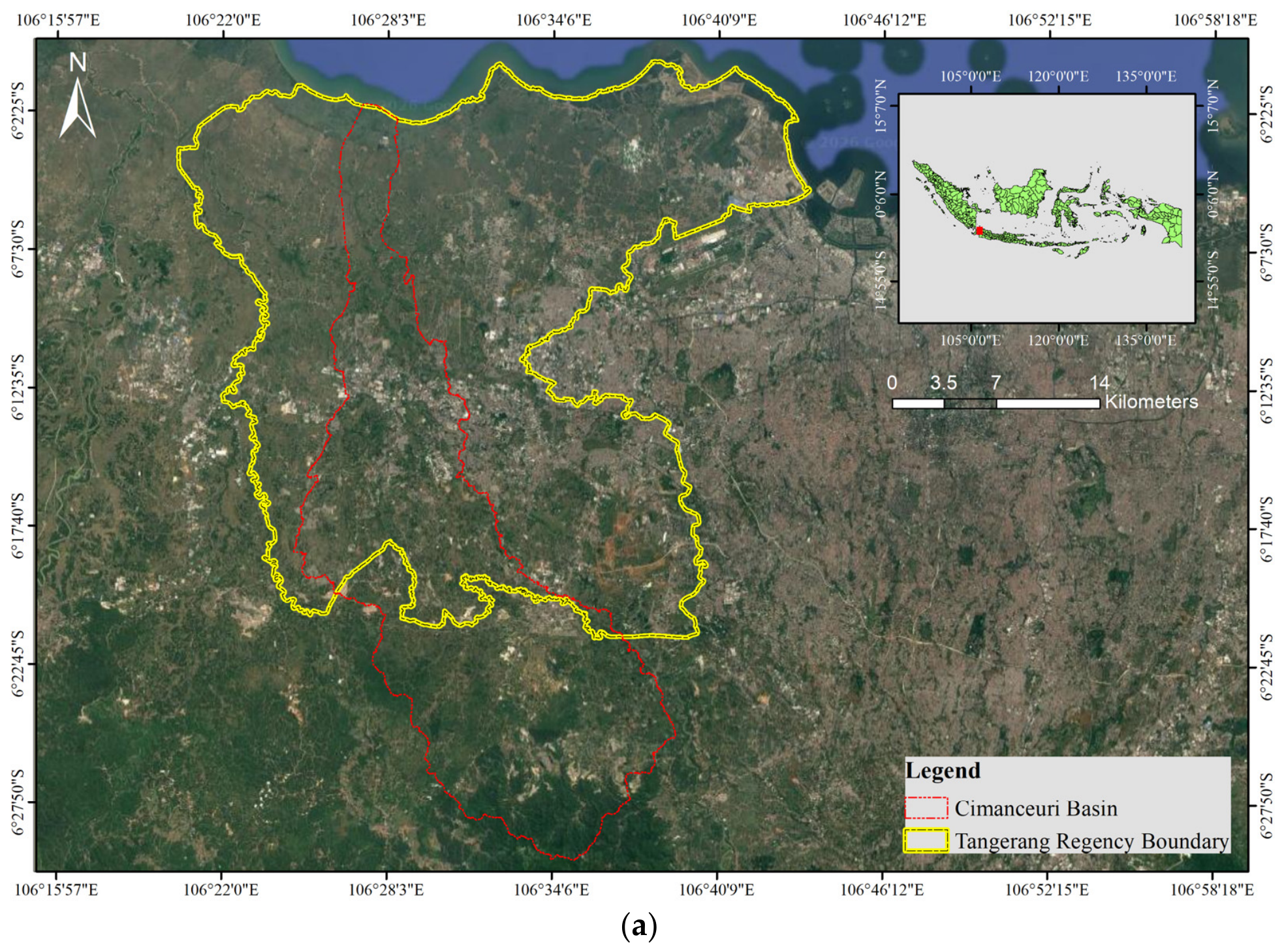
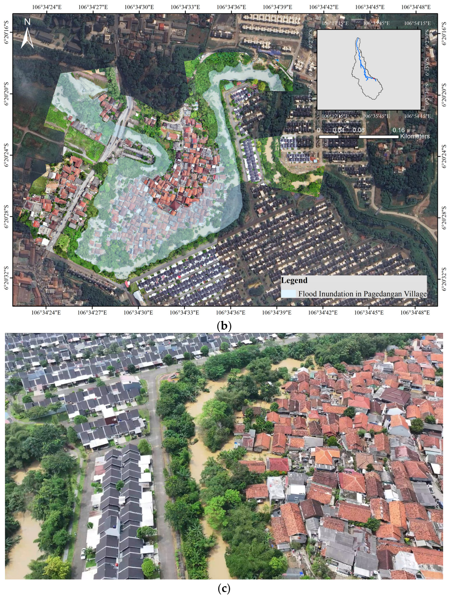
This study focuses on a selected subbasin of the Cimanceuri River, located in Tangerang Regency, Indonesia (Figure 1), as a representative area for evaluating the influence of DEM spatial resolution on flood inundation modelling performance. The subbasin was selected due to the frequent occurrence of flood events. These characteristics make it suitable for assessing variations in flood extent and hydraulic behavior under different DEM resolutions.

This study focuses on a selected subbasin of the Cimanceuri River located in Tangerang Regency, Banten Province, Indonesia (Figure 1), with a watershed area of approximately 490.34 km². The study area was selected because it frequently experiences flood events caused by intense rainfall, rapid urban development, land-use change, and limited drainage capacity. In addition, the availability of high-resolution LiDAR data and observed inundation records from the 3 March 2025 flood event makes this area suitable for evaluating the influence of DEM spatial resolution on flood inundation modelling performance.

The region has a tropical monsoon climate characterized by distinct wet and dry seasons. Based on long-term rainfall records from 2001 to 2024, the mean annual rainfall is approximately 2098 mm/year, indicating relatively high rainfall intensity with notable interannual variability. The mean annual potential evapotranspiration is approximately 1560 mm/year based on previous hydrological research conducted in the regional setting [26]. The relatively flat topography and ongoing urban expansion make the basin highly vulnerable to both pluvial and fluvial flooding. In this study, the selected basin can be characterized as a low-relief, urbanizing tropical catchment, where relatively small elevation differences play an important role in controlling floodplain connectivity and flow pathways. As a result, the study area is expected to exhibit relatively high sensitivity to DEM spatial resolution.

2.2. Methodology

This study employs an integrated hydrological–hydraulic modelling framework to evaluate the influence of different DEM spatial resolutions on flood inundation accuracy and computational efficiency within a selected subbasin of the Cimanceuri River in Tangerang Regency, Indonesia. As a preliminary step, hydrological analysis was conducted to estimate the flood discharge hydrograph required for hydraulic simulations. The hydrological modelling was performed using HEC-HMS version 4.13 to simulate rainfall–runoff processes and to derive the flood hydrograph associated with the observed flood event on 3 March 2025. The resulting hydrograph represents the estimated flood discharge at the upstream boundary and was subsequently used as the primary input for hydraulic modelling in the Hydrologic Engineering Center’s River Analysis System (HEC-RAS) version 6.6, using the 1D modelling approach. To isolate the effect of DEM spatial resolution, land use and hydrological parameters (e.g., Curve Number and Manning’s roughness coefficient) were kept constant across all simulations. Under this controlled modelling framework, differences in inundation extent and computational performance can be primarily attributed to variations in terrain resolution rather than surface variability.

A LiDAR-derived DEM was used as the primary elevation dataset and resampled into eight spatial resolutions to assess its impact on hydraulic modelling performance. Hydrological inputs, including rainfall data and the derived flood discharge hydrograph from the hydrological model, were applied consistently across all DEM scenarios to maintain comparability between simulations. For each DEM resolution, hydraulic geometries were generated and unsteady flow simulations were conducted under identical modelling configurations.

Model calibration was carried out using aerial imagery from the 3 March 2025 flood event in Pagedangan Village. The observed flood extent and water depth patterns extracted from the imagery were compared with simulated inundation maps produced by the hydraulic models. Model performance was evaluated based on flood inundation extent, water depth distribution, and computational time across different DEM scenarios, enabling an assessment of the relationship between model accuracy and computational efficiency for both 1D and 2D hydraulic simulations. To quantitatively assess the difference between simulated and observed inundation extent, the inundation area deviation (ΔA) was calculated as follows:

$$\Delta \mathrm{A}={\displaystyle \frac{\mid A_{sim}-A_{obs}\mid }{A_{obs}}}\times 100\%$$

where $A_{sim}$ is the simulated inundation area and $A_{obs}$ is the observed inundation area derived from aerial imagery. Lower values of ΔA indicate better agreement between simulation and observation.

The overall modelling workflow therefore consisted of hydrological analysis to derive the flood discharge hydrograph, DEM preprocessing and resampling, hydraulic geometry development, boundary condition configuration, unsteady flow simulation, calibration and validation, and performance evaluation.

Prior to the DEM resolution comparison, hydraulic calibration was performed using the observed flood event of 3 March 2025. The calibration focused on adjusting Manning’s roughness coefficient (n) within physically reasonable ranges to achieve agreement between simulated and observed flood conditions derived from aerial imagery and field documentation. Hydrological parameters, including curve number (CN) and lag time, were assigned based on standard methods and literature values and were not subject to calibration. Model performance was evaluated based on the agreement of inundation extent, flood patterns, and consistency of peak flow timing.

To ensure comparability among DEM resolution scenarios, the calibrated parameter set was kept constant for all simulations, and only the DEM spatial resolution was varied. This approach isolates the effect of DEM resolution from parameter uncertainty. The 3 March 2025 event was selected because it was one of the most significant recent flood events in the study area and had the most complete supporting observational data, including rainfall records and aerial imagery. Although this study focuses on a single event, it is considered representative of event-based urban flooding caused by intense rainfall in the basin. The selection of this event was primarily constrained by the availability of reliable inundation extent data derived from aerial imagery, which is essential for model validation. Additional rainfall events were not included due to the lack of comparable observed inundation datasets. However, model sensitivity to DEM resolution may vary under rainfall events with different total depths, peak intensities, durations, and temporal rainfall distributions. Therefore, future studies using multiple storm events are recommended to further evaluate the robustness of the identified DEM-performance relationship.

2.3. Data Collection

2.3.1. Digital Elevation Model (DEM)

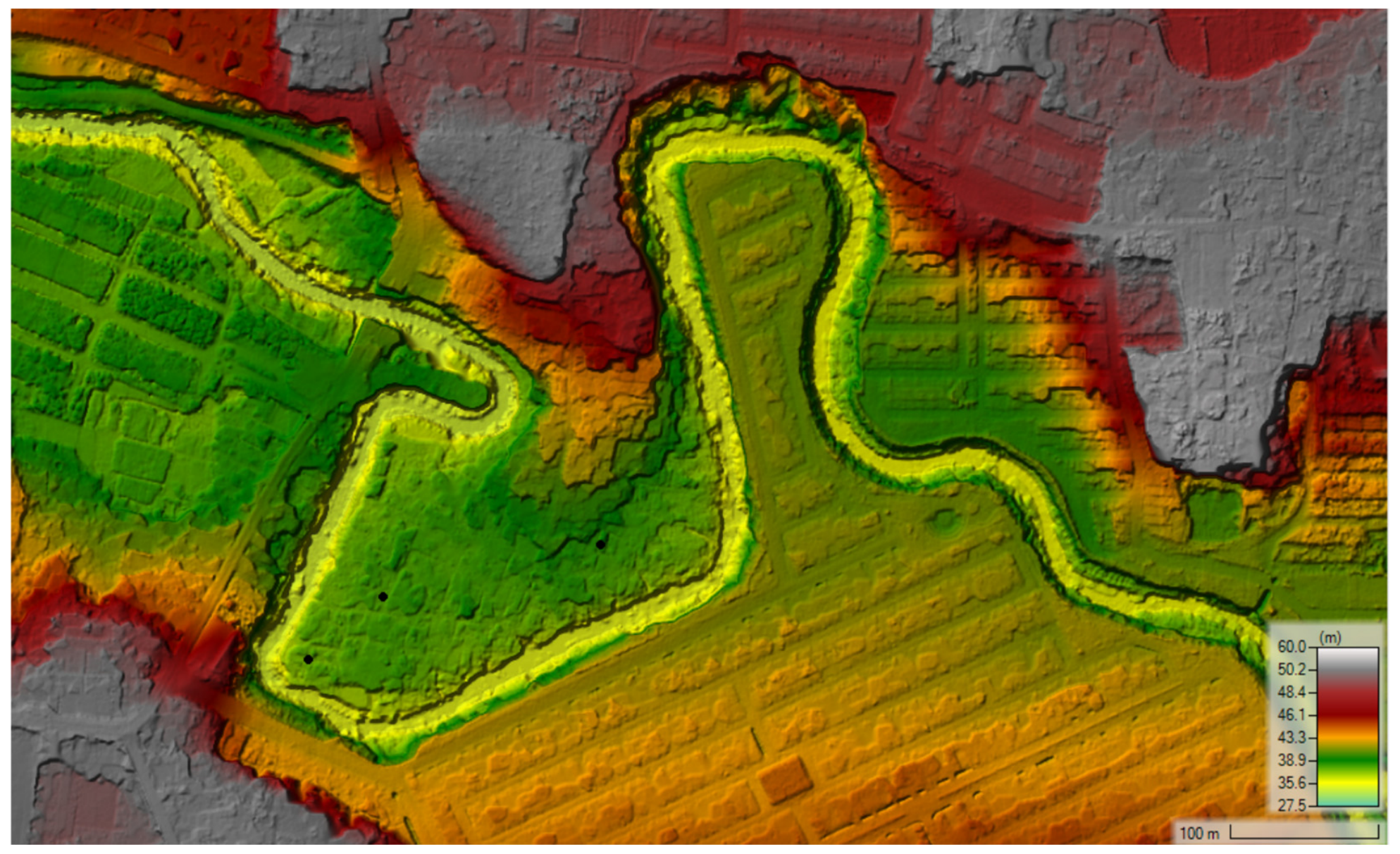
Topographical information was derived from a DEM provided by the Public Works and Water Resources Agency of Tangerang Regency. River geometry and land surface elevation were derived from high-resolution LiDAR 1 m data to represent detailed terrain characteristics within the study area of the Cimanceuri River, Tangerang Regency. The original LiDAR DEM 1 m (Figure 2) was treated as the reference elevation dataset due to its high vertical and horizontal accuracy.

To evaluate the influence of spatial resolution on hydraulic modelling performance, the 1 m LiDAR-derived DEM was systematically resampled into multiple grid sizes: 2 m, 5 m, 8 m, 10 m, 20 m, 25 m and 30 m. The resampling process was conducted using bilinear interpolation to preserve terrain continuity while reducing spatial detail [27,28]. From each DEM resolution, river centerlines, bank lines, and cross-sectional geometries were extracted and imported into HEC-RAS for 1D model development. For the 2D simulations, each DEM resolution was directly used to generate computational terrain surfaces and flow area meshes. This controlled modelling framework ensured that terrain representation was the only variable modified across simulation scenarios, while hydraulic parameters and boundary conditions remained constant, enabling systematic assessment of DEM resolution effects on flood modelling performance [24].

2.3.2. Land Use

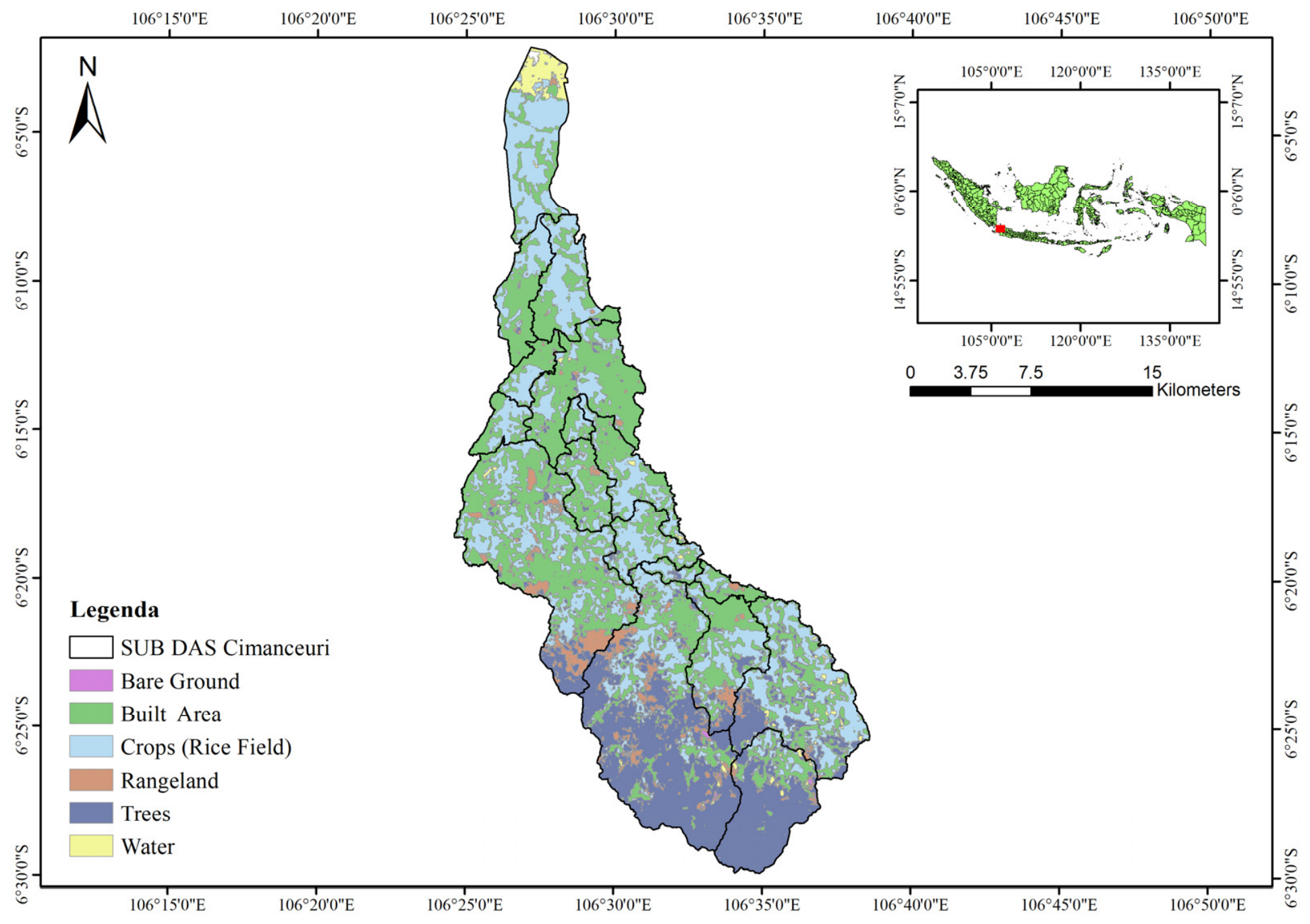
Land use information was derived from the 2024 ESRI Sentinel-2 Land Cover dataset to characterize watershed surface conditions and support the estimation of runoff and infiltration dynamics [9]. This dataset provides recent and consistent land cover classification derived from Sentinel-2 imagery and was utilized to represent current watershed surface conditions within the study area of the Cimanceuri River in Tangerang Regency. The land cover map was used to determine watershed characteristic parameters that influence hydrological processes, particularly surface runoff generation and infiltration capacity. The resulting land cover distribution of the study area is presented in Figure 3, illustrating the dominance of built-up areas, vegetation, agricultural land, and other surface classes used for parameter assignment in the hydrological and hydraulic models.

Land cover classes were reclassified into major categories relevant to hydrological and hydraulic modelling, such as built-up areas, vegetation, agricultural land, open spaces, and water bodies. These classes were subsequently used to assign hydrological parameters, including Curve Number (CN) values for rainfall–runoff modelling in HEC-HMS and Manning’s roughness coefficients (n) for hydraulic simulations in HEC-RAS [29]. The mapping between land use classes and the assigned Curve Number (CN) values and Manning’s roughness coefficients used in the hydraulic simulations are provided in the Supplementary Materials (Table S1) [30]. Unlike the DEM datasets, which were systematically resampled to evaluate spatial resolution effects, the land use dataset was maintained at its original resolution across all modelling scenarios. This ensured that differences in flood inundation results were attributed solely to variations in DEM spatial resolution rather than changes in land surface characteristics.

2.3.3. Rainfall Data

The hydrological analysis was performed to quantify the rainfall–runoff response and to generate the flood discharge hydrograph required for hydraulic modelling within the Cimanceuri subbasin. The procedure consisted of two main stages, rainfall temporal disaggregation and rainfall–runoff transformation using HEC-HMS.

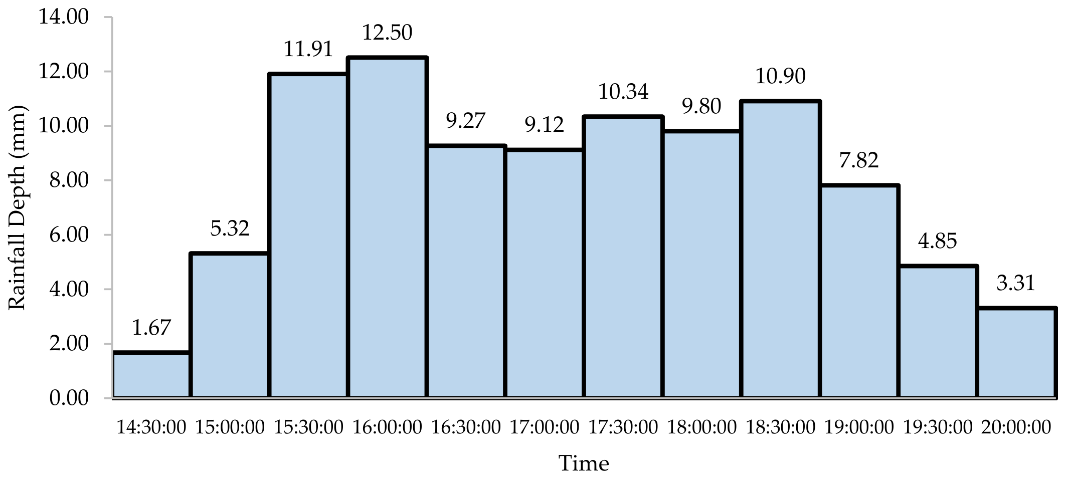
Rainfall data for the 3 March 2025 flood event were obtained from the Badan Meteorologi Klimatologi dan Geofisika (BMKG) Budiarto meteorological station. As HEC-HMS requires sub-daily rainfall inputs to accurately simulate runoff dynamics and peak discharge, the observed daily rainfall totals were temporally disaggregated into 30-min intervals. The disaggregation proportions were derived from bias-corrected Global Precipitation Measurement (GPM) satellite data as shown in Figure 4. Nevertheless, uncertainty may remain in representing short-duration rainfall peaks and storm timing, which could influence simulated runoff responses.

Previous studies have demonstrated that bias correction significantly improves the agreement between satellite-based rainfall estimates and ground observations, thereby enhancing their reliability for hydrological applications [31]. By integrating ground-based daily totals with bias-adjusted satellite-derived temporal patterns, this approach preserves observational accuracy while improving temporal resolution for runoff modelling.

Table 2. GPM rainfall distribution weight at 30 min intervals.

Date	Time	GPM Rainfall Distribution Weight (%)
		Subbasin 1	Subbasin 2	Subbasin 3	Subbasin 4	Subbasin 5	Subbasin 6	Subbasin 7	Subbasin 8
3 March 2025	14:30:00	0.03	0.02	0.01	0.01	0.02	0.01	0.01	0.01
	15:00:00	0.06	0.06	0.05	0.05	0.06	0.05	0.05	0.04
	15:30:00	0.14	0.16	0.11	0.11	0.11	0.11	0.10	0.09
	16:00:00	0.12	0.15	0.13	0.13	0.12	0.13	0.13	0.14
	16:30:00	0.08	0.09	0.10	0.10	0.09	0.10	0.11	0.17
	17:00:00	0.08	0.09	0.10	0.11	0.09	0.11	0.11	0.14
	17:30:00	0.10	0.10	0.11	0.11	0.11	0.11	0.11	0.11
	18:00:00	0.10	0.09	0.11	0.11	0.10	0.11	0.11	0.10
	18:30:00	0.12	0.10	0.11	0.11	0.12	0.11	0.11	0.08
	19:00:00	0.08	0.08	0.08	0.08	0.09	0.08	0.08	0.06
	19:30:00	0.05	0.05	0.05	0.05	0.06	0.05	0.05	0.03
	20:00:00	0.03	0.03	0.03	0.03	0.04	0.03	0.03	0.02
Total		1.00	1.00	1.00	1.00	1.00	1.00	1.00	1.00

presents normalized dimensionless weights for each 30-min interval, with values in each subbasin summing to 1.00. These weights were derived from Global Precipitation Measurement (GPM) data for the 3 March 2025 flood event. Based on the GPM time series, rainfall occurred between 14:30 and 20:00 local time. The cumulative rainfall over this period was calculated and disaggregated into 30-min intervals, and the weights for each subbasin were determined based on the proportional rainfall contribution within each interval.

3. Results and Discussion

3.1. Hydrology Analysis

The hydrological simulation was configured in HEC-HMS by integrating the Basin Model, Meteorological Model, Control Specifications, and Time Series Data components to represent the rainfall–runoff processes within the Cimanceuri subbasin. The basin was schematized into representative subbasins (SS), and key hydrological parameters were assigned consistently across the modelling framework. These included the selected loss method, transform method, and baseflow representation to characterize infiltration, surface runoff generation and flow routing processes.

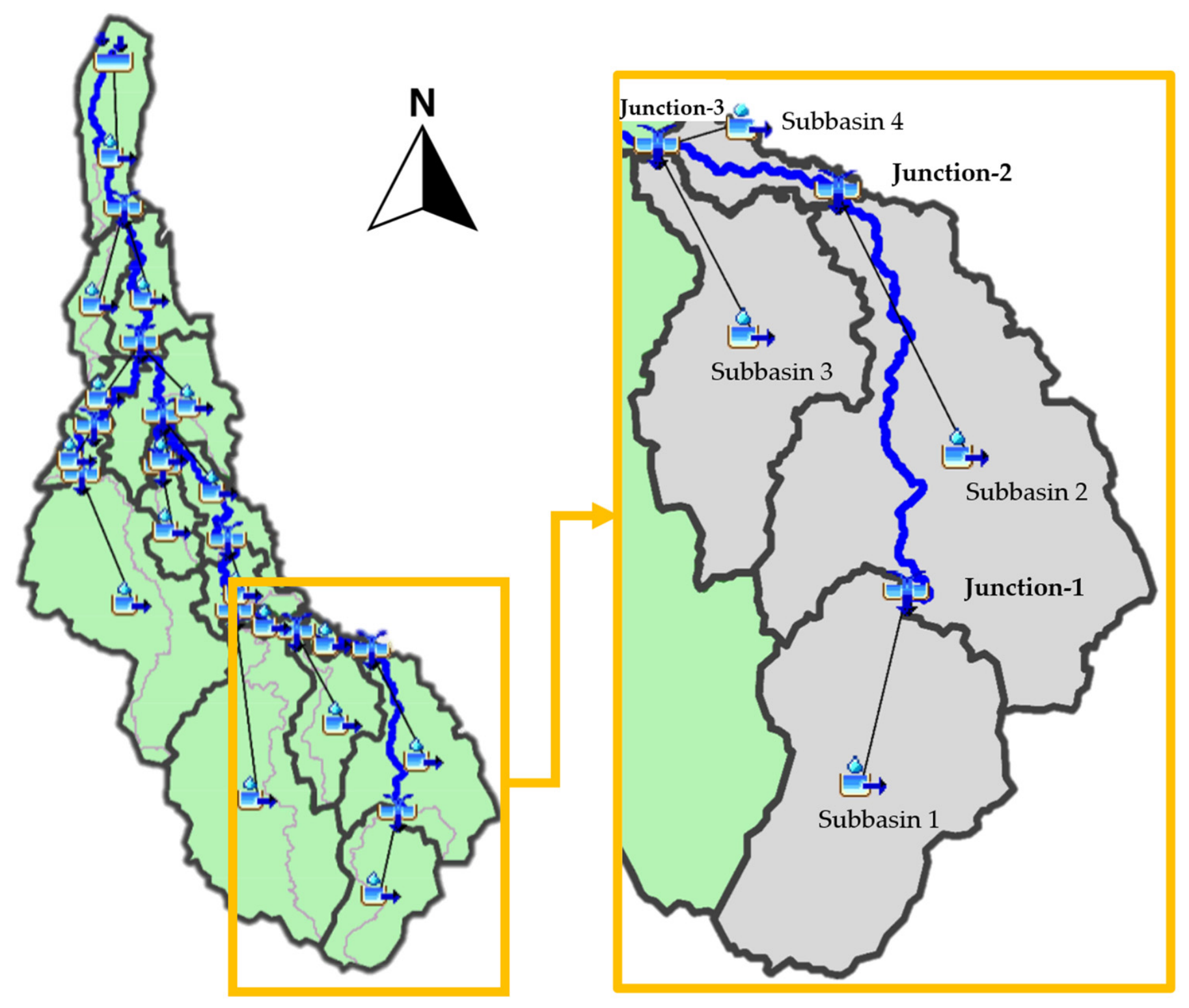
The calculation of flood discharge for inundation modelling purposes considered the cumulative flow contributions from upstream subbasins relative to the inundation point. The simulated discharge represents the estimated surface runoff generated by rainfall over these upstream areas, thereby reflecting the volume of water with the potential to cause flooding at the study site in Karang Tengah Village, Pagedangan Sub-district. For the 3 March 2025 event-based modelling, the discharge analysis focused on Junction 3 as a key hydraulic control point within the basin system. Junction 3 represents the confluence points between upstream subbasins in the HEC-HMS model, where flow from Subbasins 1, 2, and 3 is combined before entering Subbasin 4. The study area is located in Subbasin 4, which serves as the downstream outlet of the system. Therefore, the discharge hydrograph used as input for hydraulic modelling reflects the cumulative contribution of upstream subbasins through Junction 3. A visual representation of the Cimanceuri sub-watershed basin configuration is presented in Figure 5.

Subbasin (SS) parameters such as curve number (CN), lag time, and initial abstraction were defined based on land cover characteristics, watershed morphology, and standard hydrological estimation approaches. The meteorological model incorporated the temporally disaggregated rainfall data, while the control specifications defined the simulation time window corresponding to the 3 March 2025 flood event. Composite curve number (CN) values for each subbasin were estimated using an area-weighted approach based on the proportion of each land use class within the subbasin. The detailed land use composition and parameter values are provided in the Supplementary Materials (Table S2).

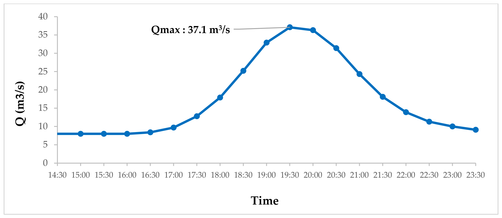
After defining all model components and subbasin parameters, the simulation was executed to evaluate the rainfall–runoff response of the watershed. The resulting discharge hydrograph at the selected outlet was analyzed to assess peak flow magnitude and temporal runoff behavior. Based on the simulation results, the peak discharge was estimated to be approximately 37.1 m³/s (Figure 6). The hydrograph exhibits a gradual rising limb, a distinct peak, and a recession phase, reflecting the hydrological response time of the Cimanceuri subbasin to high-intensity rainfall. The simulated discharge hydrograph was subsequently applied as the upstream boundary condition in the hydraulic modelling stage to ensure consistency between hydrological and hydraulic analyses.

The simulated discharge hydrograph was subsequently applied as the upstream boundary condition in the hydraulic modelling stage to ensure consistency between hydrological and hydraulic analyses.

It should be noted that the absence of continuous discharge observations introduces uncertainty in the quantitative evaluation of the simulated hydrograph. However, the simulated peak discharge and timing remain consistent with observed flood conditions and inundation patterns derived from aerial imagery, suggesting that the model provides a reasonable representation of the hydrological response for the selected event.

3.2. Hydraulic Modelling Processes

The discharge hydrograph generated from the hydrological modelling (Figure 6) was consistently applied as the upstream boundary condition in both 1D and 2D simulations. No modifications were made across DEM scenarios to ensure that differences in inundation results were solely attributed to terrain resolution. Hydraulic flood modelling was performed to assess the influence of DEM resolution on inundation accuracy and computational efficiency. The simulations were conducted using HEC-RAS, applying both 1D and 2D approaches to represent the flood event of 3 March 2025 in an urban area.

Due to the limited availability of continuous discharge gauge records within the Cimanceuri subbasin, direct quantitative validation of the hydrological model using statistical performance metrics could not be performed. Therefore, model calibration was conducted using an event-based approach, relying on indirect validation through consistency between the simulated discharge hydrograph and the observed flood extent derived from aerial imagery, as well as reported flood timing and field observations [32].

3.2.1. HEC-RAS 1D Flood Modelling

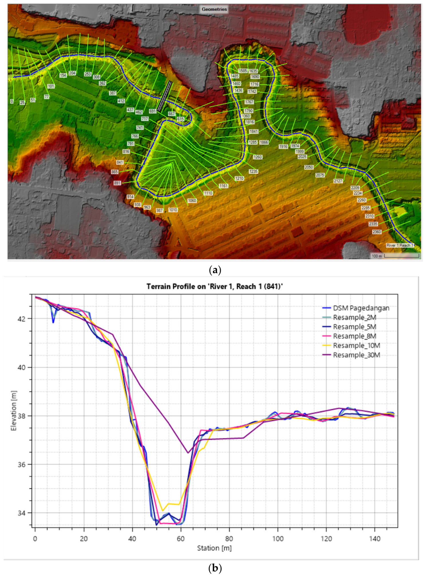
The 1D hydraulic model geometry was developed from LiDAR-derived DEMs at each spatial resolution. River centerlines were digitized, and cross-sections were extracted from multiple terrain data resolutions (Figure 7). Subsequently, bank stations were identified to differentiate the main channel and overbank areas.

The cross-sections used in the HEC-RAS model (Figure 7a) were generated from the LiDAR using the terrain processing tools in HEC-RAS. Cross-section cut lines were defined along the river reach at an average spacing of approximately 9–33 m, depending on channel curvature and topographic variation. In relatively straight reaches, wider spacing was applied, while in areas with significant geometric changes (e.g., bends or slope transitions) closer spacing was used to better capture channel morphology.

The elevation profiles of each cross-section were directly extracted from the DEM for each resolution scenario. Therefore, differences in cross-sectional geometry are inherently influenced by the spatial resolution of the DEM.

Figure 7b illustrates a representative cross-section along Reach 1, which refers to the model reach name assigned to the Cimanceuri River within the HEC-RAS geometry setup. The variation in cross-sectional shape reflects the influence of different DEM resolutions, where higher-resolution DEMs capture more detailed channel geometry, while lower-resolution DEMs tend to produce smoother and simplified profiles.

Higher-resolution DEMs are able to represent finer topographic features, resulting in more detailed and irregular cross-section profiles. In contrast, lower-resolution DEMs tend to smooth the terrain, which can lead to simplified channel geometry, reduced bank definition and potential underestimation or overestimation of flow area.

These variations directly affect hydraulic properties such as wetted area and flow conveyance, which in turn influence the simulation results in HEC-RAS.

The model was configured as an unsteady flow simulation representing the 3 March 2025 flood event, with an event-based inflow hydrograph applied as the upstream boundary condition and a normal depth condition at the downstream boundary.

A uniform Manning’s roughness coefficient (n) was applied along the modeled reach, and its value was determined based on both calibration results and the physical characteristics of the river. The Cimanceuri River within the study area is characterized by a natural channel with irregular cross-sections, vegetated banks and moderate floodplain interaction.

To ensure robustness, the selected value was further supported by a previous study conducted in the same river system, namely “Flood Inundation Mapping in the Cimanceuri River through Integration of HEC-HMS and HEC-RAS as a Basis for Flood Risk Management”. In that study, calibration was performed using LiDAR-derived terrain data and the flood event of 3 March 2025 by testing several Manning’s n values (0.035, 0.1, 0.2 and 0.3). The results indicated that a value of 0.035 significantly underestimated inundation extent, while 0.300 led to overestimation. The value of 0.200 produced the closest agreement between simulated and satellite-observed flood extent [9].

Based on both the hydraulic characteristics of the river and the prior calibrated results, a uniform Manning’s n value of 0.2 was adopted in this study. This value is considered representative of the channel roughness and ensures consistency with previously validated modeling efforts in the same location.

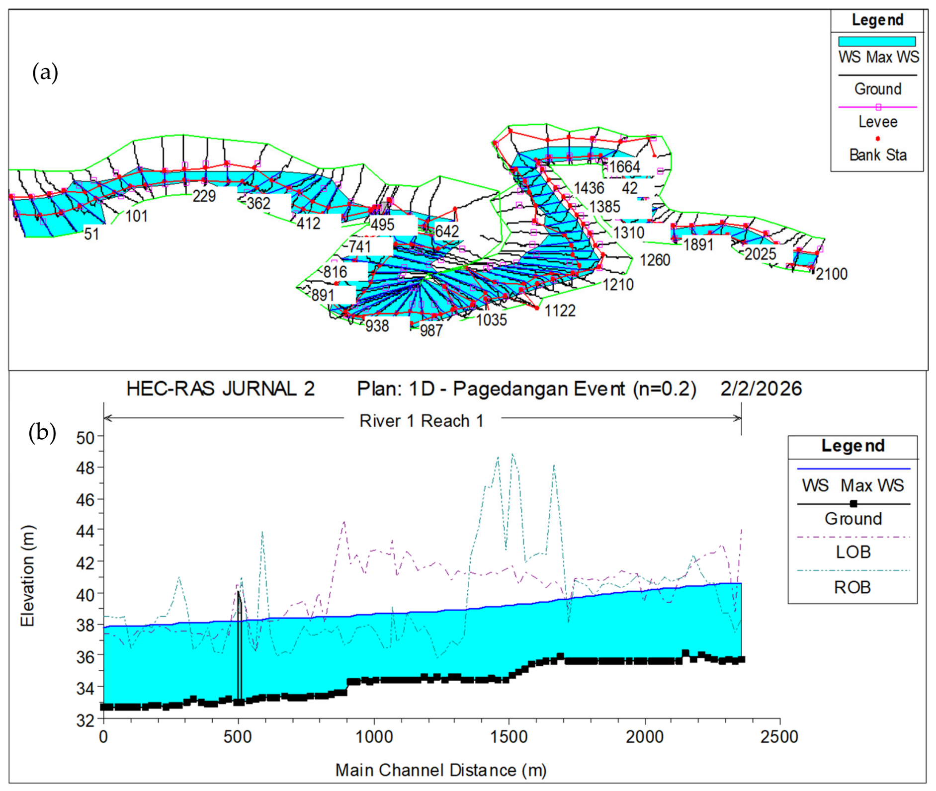
Figure 8 shows the extracted cross-sections and bank station delineation along the river, and the longitudinal water surface profile from the 1D HEC-RAS simulation. The results indicate that the model captures channel geometry and overbank areas effectively, with the simulated water surface following the river profile and indicating localized overbank flow.

3.2.2. HEC-RAS 2D Flood Modelling

In the 2D framework, the shallow water equations are solved within each computational cell, making terrain elevation a key control on flow distribution, whereas the 1D model represents flow through cross-sectional geometry with lower spatial sensitivity [5]. Previous studies have shown that higher DEM resolutions increase mesh density and computational demand in distributed flood modelling [15].

The 2D hydraulic simulations were performed in HEC-RAS 6.6 using LiDAR-derived terrain for each DEM resolution. A computational mesh was generated to represent the river channel and floodplain, with a general cell spacing of 10 × 10 m and refined 2 × 2 m break lines along the main channel to better capture hydraulic gradients and channel curvature. The upstream inflow boundary condition was defined using the discharge hydrograph obtained from the hydrological simulation of the flood event on 3 March 2025. This hydrograph represents the temporal variation of inflow discharge entering the study reach during the flood event and was used as the primary driving input for the hydraulic simulations. To represent surface resistance within the hydraulic model, a uniform Manning’s roughness coefficient of n = 0.20 was applied. This value was selected to account for the relatively high flow resistance within the study area, which is characterized by irregular floodplain topography, dense vegetation, and the presence of urban features that increase hydraulic roughness during overbank flow conditions.

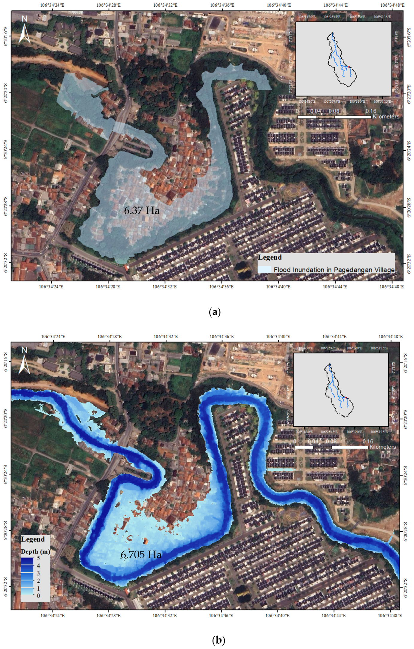
Flood inundation simulations were conducted for all DEM resolutions, producing outputs such as water depth distribution, water surface elevation, and inundation extent. Model calibration was conducted by comparing simulated inundation patterns with observed flood extents from aerial imagery. The Manning roughness coefficient used in the 2D model was also 0.20, applied consistently to represent the physical characteristics of the study area and to ensure comparability with the 1D modelling results. As shown in Figure 9, the inundation analysis was conducted using aerial imagery acquired on 3 March 2025 and a two-dimensional hydraulic model developed in HEC-RAS based on a 1 m LiDAR DEM with a Manning’s roughness coefficient of 0.2.

3.3. Comparative Role of 1D and 2D Modelling

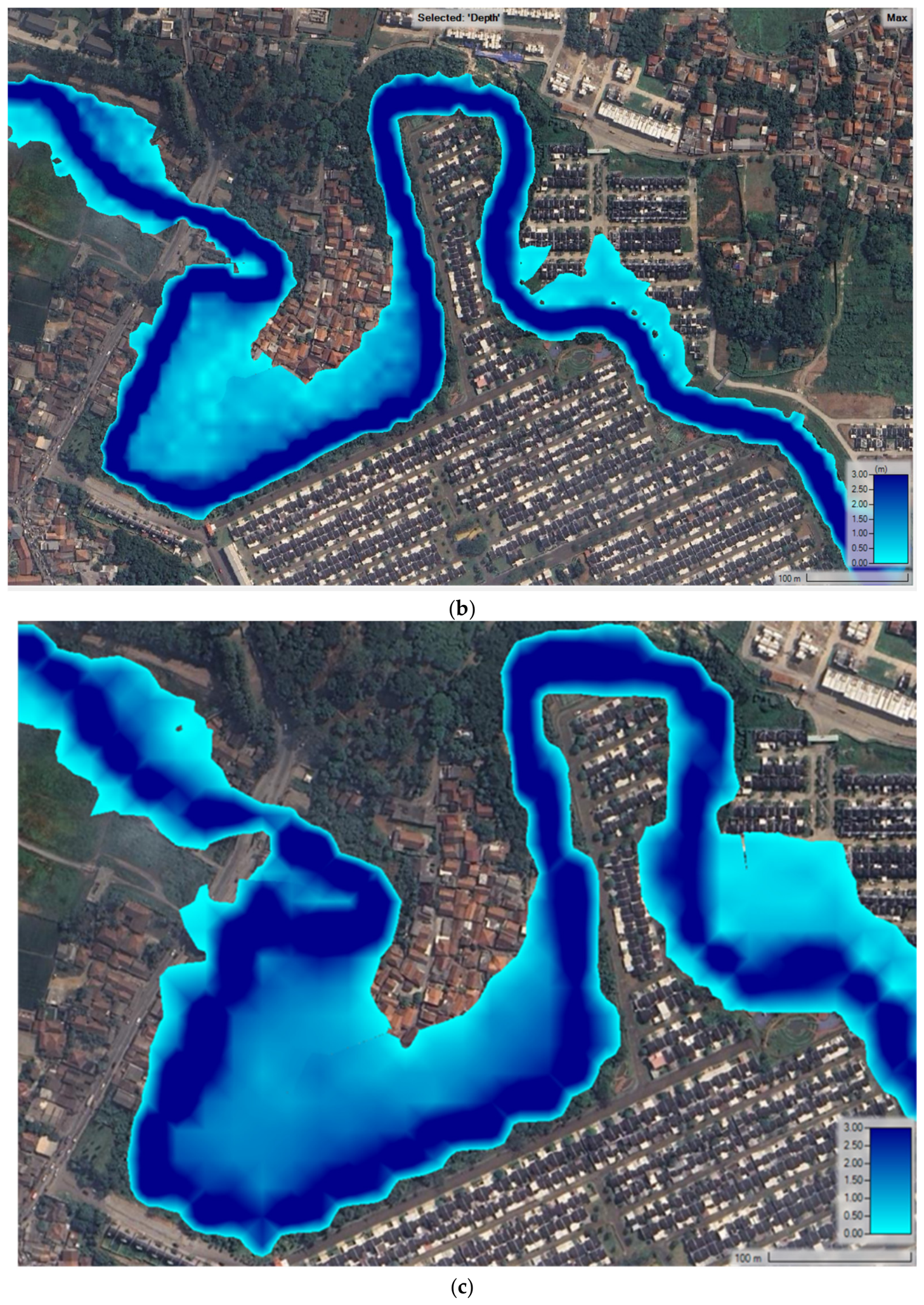
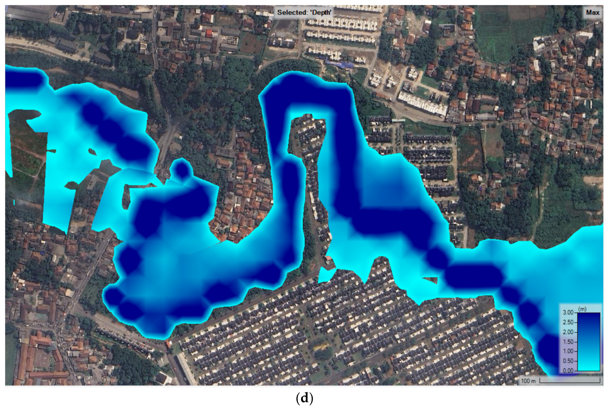
In the 1D modelling framework, the flood inundation extent was derived from simulated water surface elevation profiles along river cross-sections. The computed water surface elevation was laterally interpolated between adjacent cross-sections, and areas where the water level exceeded ground elevation were classified as inundated using the floodplain mapping tool in RAS Mapper. The total inundation area was then calculated from the generated flood polygon as shown in Figure 10. Because the 1D model represents flow using cross-sectional geometry rather than fully distributed terrain cells, variations in DEM resolution influence the extracted cross-section shape. Coarser DEMs tend to smooth channel and floodplain topography, resulting in wider and shallower effective cross-sections that may produce larger simulated inundation extents. This trend is reflected in

Table 3. Evaluation of 1D Modelling Performance and Inundation Area Overlay with Observations.

LiDAR’s Resolution (m) (a)	Computation Time (s) (b)	Inundation Area 1D (ha) (c)	Inundation Area Overlay (ha) (d)	Inundation Area Observation (ha) (e)	∆ (ha) (c–e)	FIT (%) (f) [(c + e)/d]
1	5	0.99	6.14	0.23	0.76	0.20
2	5	0.97	6.18	0.19	0.78	0.19
5	5	1.08	6.25	0.12	0.96	0.19
8	5	1.12	6.25	0.12	1.00	0.20
10	4	1.19	6.25	0.12	1.08	0.21
20	4	1.91	6.24	0.13	1.78	0.33
25	4	2.39	6.27	0.10	2.30	0.40
30	4	2.69	6.17	0.20	2.50	0.47

, where the simulated flood area increases progressively with decreasing DEM resolution. The 1D modelling approach is computationally efficient for analyzing longitudinal water surface profiles and channel flow behavior, and computation time remains relatively short and stable across all DEM scenarios. However, despite its efficiency, the 1D approach has limitations in representing complex floodplain dynamics, particularly in urban environments, which may contribute to deviations between simulated and observed inundation areas.

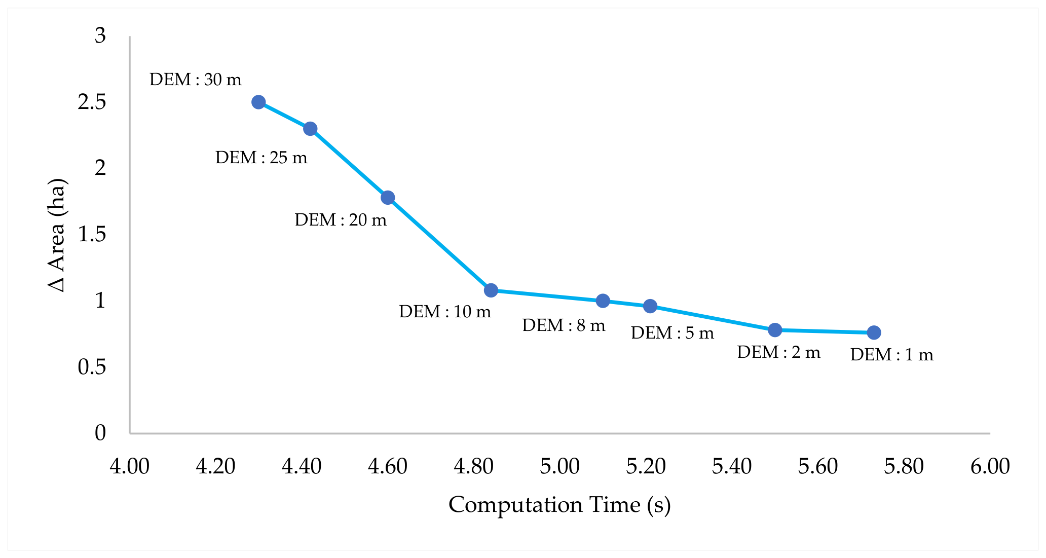
Figure 11 shows the relationship between inundation area deviation (ΔA) and computational time in the 1D simulations. The computation time remains relatively stable across all DEM resolutions (approximately 4–5 s) indicating that the 1D model is computationally robust and not strongly affected by terrain resolution. However, ΔA increases progressively as DEM resolution becomes coarser, reflecting the gradual loss of spatial detail. A noticeable inflection point appears around the 10 m resolution, where deviation remains moderate while computation time is already low and stable. Beyond this point, deviation increases more substantially without significant computational benefit. Therefore, the 10 m DEM represents the most balanced compromise between acceptable accuracy and computational efficiency in the 1D framework.

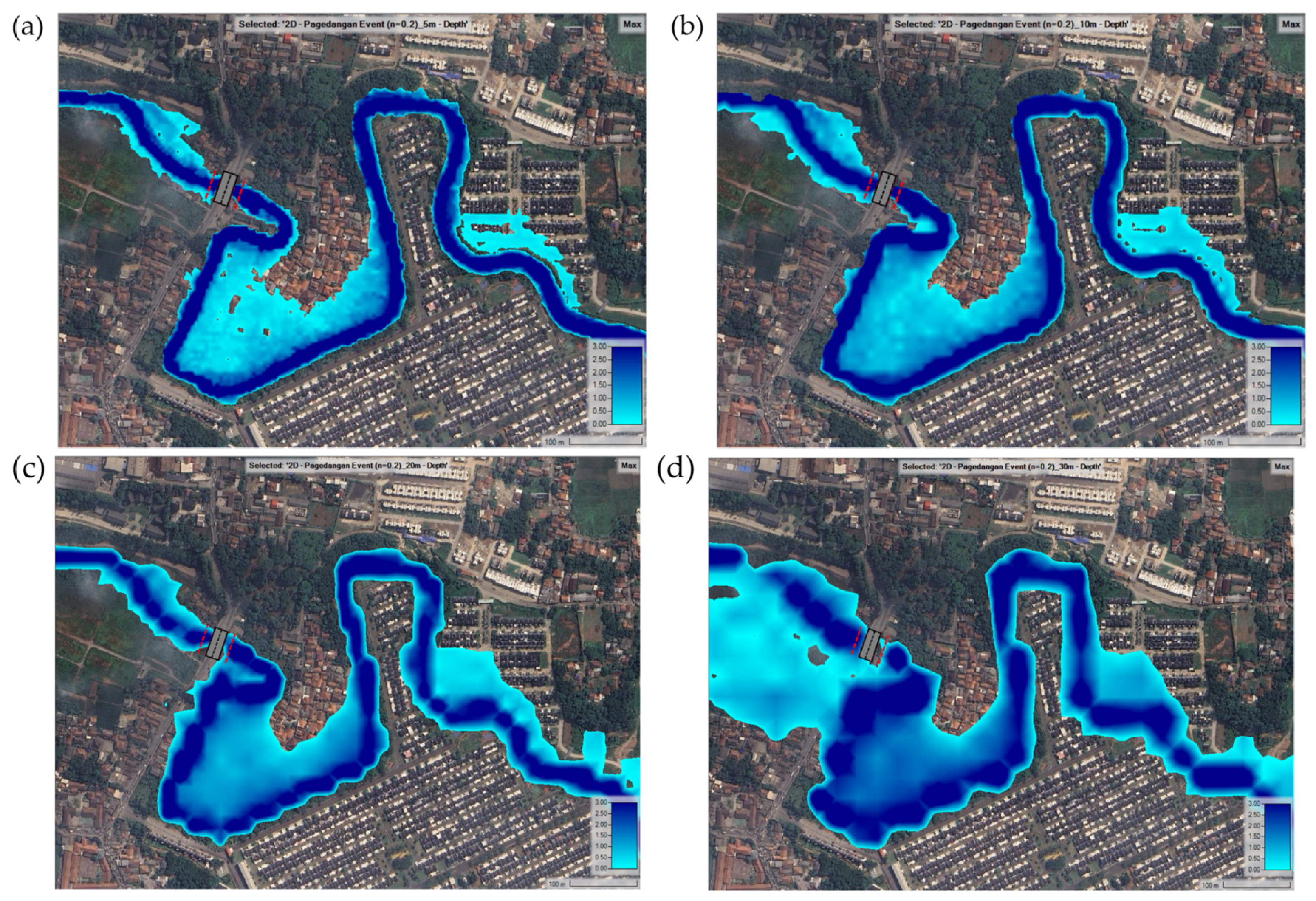
A similar pattern is observed in the 2D simulations. Although computation time decreases progressively as DEM resolution becomes coarser, the deviation from observed inundation increases at a faster rate beyond the 10 m resolution. The curve indicates a transitional point around 10 m, where deviation remains relatively moderate (0.63 ha) while computational time has already been substantially reduced compared to finer resolutions.

The 2D simulations demonstrate higher sensitivity to DEM resolution. Although computation time decreases from 20:34 at 1 m to 13:54 at 30 m, it remains substantially higher than that of the 1D model. Deviation from observed inundation increases as DEM resolution becomes coarser, rising from 0.33 ha at 1 m to 3.12 ha at 30 m (

Table 4. Evaluation of 2D Modelling Performance and Inundation Area Overlay with Observations.

LiDAR’s Resolution (m) (a)	Computation Time (min:s) (b)	Inundation Area 2D (ha) (c)	Inundation Area Overlay (ha) (d)	Inundation Area Observation (ha) (e)	∆ (ha) (c–e)	FIT (%) (f) [(c + e)/d]
1	20:34	0.71	5.99	0.38	0.33	18.20
2	17:49	0.71	6.01	0.36	0.34	17.80
5	15:56	0.76	6.07	0.30	0.46	17.50
8	15:47	0.79	6.10	0.27	0.52	17.40
10	15:44	0.88	6.11	0.26	0.63	18.70
20	14:43	1.38	5.92	0.45	0.92	31.00
25	14:21	1.67	6.16	0.21	1.46	30.50
30	13:54	3.48	6.01	0.36	3.12	0.64

). Nevertheless, the 2D model consistently produces smaller deviations than the 1D model for resolutions up to 20 m, indicating its superior ability to represent spatial floodplain flow.

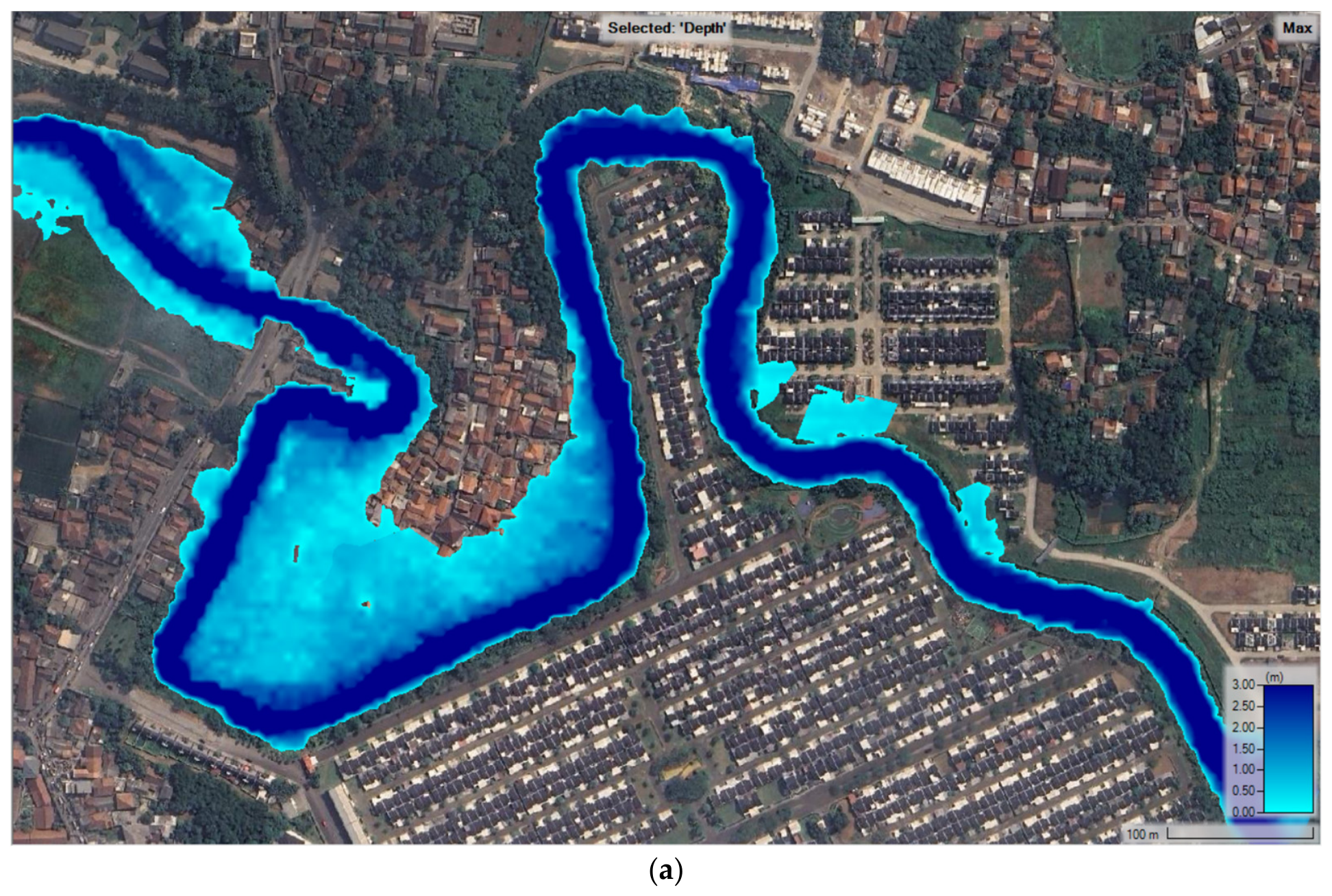
Beyond this threshold, particularly at 20 m and coarser resolutions, deviation increases sharply without proportional gains in computational efficiency. This suggests diminishing returns in model performance as terrain detail becomes overly generalized. Therefore, consistent with the 1D findings, the 10 m DEM also represents the most balanced compromise between spatial accuracy and computational demand in the 2D framework. Therefore, consistent with the 1D findings, the 10 m DEM also represents the most balanced compromise between spatial accuracy and computational demand in the 2D framework (Figure 12).

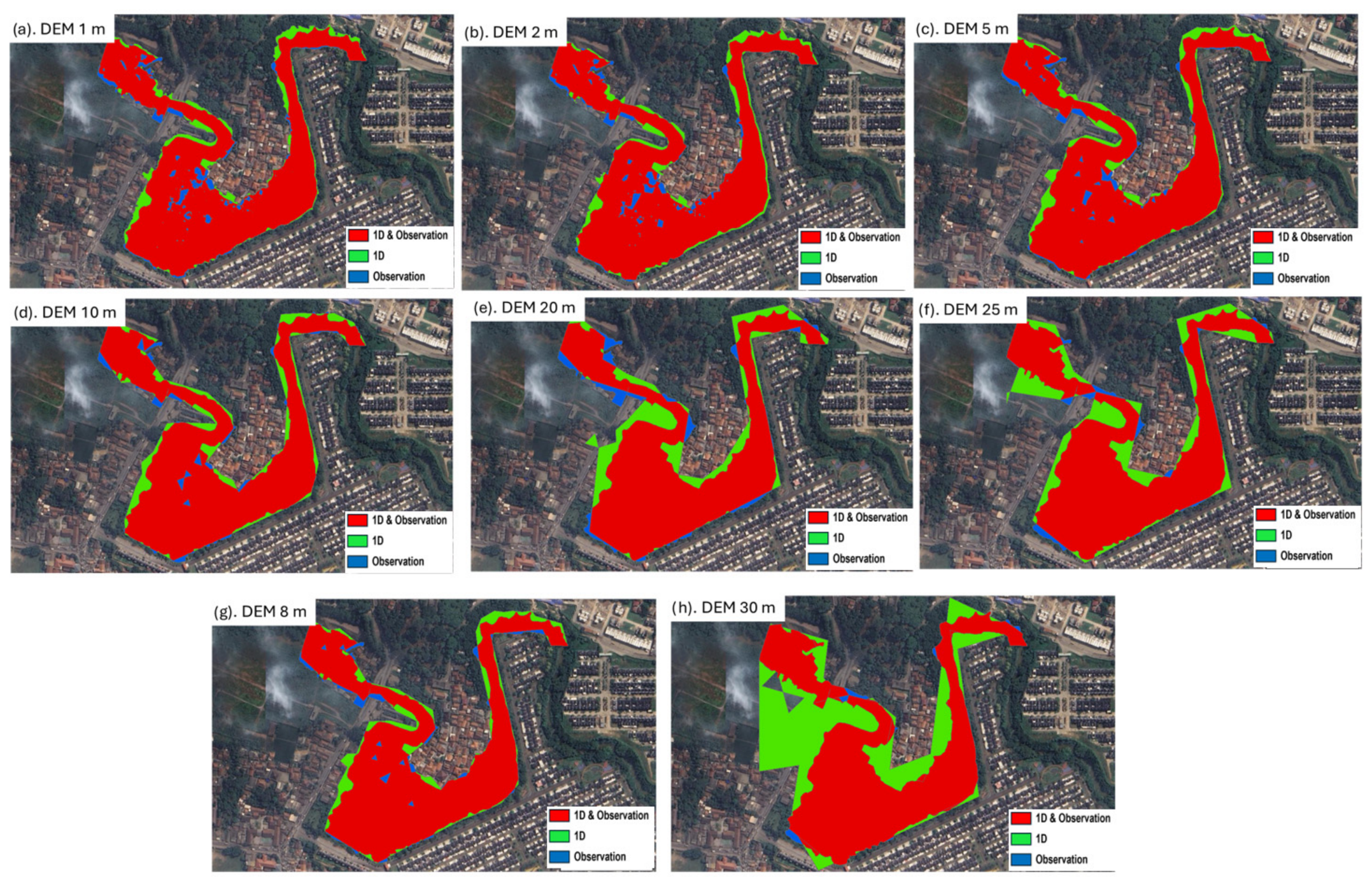
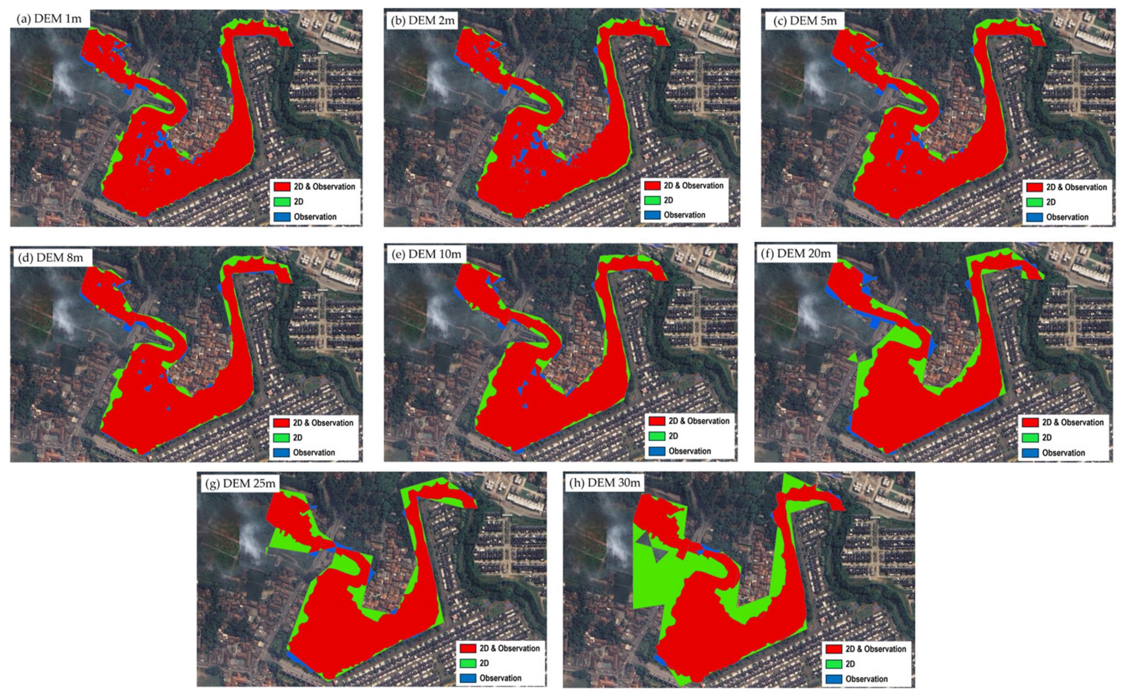
When comparing both approaches, a clear overlap in performance can be observed at intermediate resolutions. For example, at a 10 m resolution, the 1D model shows a deviation of 1.08 ha, whereas the 2D model yields 0.63 ha. Although the 2D model remains more accurate, the difference becomes less pronounced compared to very fine resolutions. This indicates that at moderate resolutions, particularly 10 m, both modelling approaches provide reasonably comparable inundation extents, with 2D offering improved spatial detail and 1D maintaining high computational efficiency (Table 3 and Table 4; Figure 13 and Figure 14).

The overlay analysis further confirms that DEM resolution influences both modelling frameworks, although the magnitude of its impact differs. Changes in DEM resolution directly affect the representation of terrain features, where finer resolutions preserve detailed channel and floodplain topography, while coarser resolutions tend to smooth elevation variability. This smoothing effect alters flow pathways and floodplain connectivity, which can lead to differences in simulated inundation extent and water depth distribution. Despite variations in the total simulated inundation area, the overlapping inundation extent between the 1D and 2D models remains relatively stable across resolutions, indicating that the core flooded zone is consistently captured by both modelling approaches.

The 2D model demonstrates higher sensitivity to terrain detail because flow dynamics are computed across distributed grid cells that directly depend on terrain representation. As DEM resolution becomes coarser, the loss of topographic detail leads to greater deviation from observed inundation patterns. In contrast, the 1D model is less sensitive to DEM resolution because it represents flow primarily through cross-sectional geometry, making it computationally more stable but inherently limited in representing complex floodplain flow dynamics.

Overall, the results highlight a clear trade-off between model accuracy and computational efficiency. While high-resolution DEMs improve the representation of terrain and flood processes, they significantly increase computational time, particularly for 2D simulations. Conversely, coarser DEMs reduce simulation time but may decrease inundation accuracy due to simplified terrain representation. Based on the results, a DEM resolution of approximately 10 m provides a practical balance between accuracy and computational efficiency, particularly for the 1D modelling framework. This finding provides practical guidance for flood modelling applications, indicating that moderate-resolution DEMs can support reliable flood inundation assessment while maintaining efficient simulation performance, which is particularly beneficial for rapid flood analysis, early warning systems, and operational flood risk management. However, the identified optimal DEM resolution of 10 m should be interpreted within the context of the Cimanceuri Basin, which is characterized by relatively flat topography and urban floodplain conditions. In steeper or more hydraulically complex catchments, finer DEM resolutions may be required.

The findings of this study are consistent with previous research highlighting the significant influence of DEM resolution on hydraulic modelling accuracy. Several studies have reported that higher-resolution DEMs generally improve the representation of channel geometry and floodplain features, leading to more accurate inundation mapping [24,33]. The results of this study confirm that finer DEM resolutions produce more detailed cross-sectional geometry and improved inundation extent agreement, as reflected by lower ΔA values.

However, in line with previous findings, increasing DEM resolution also leads to higher computational demand, particularly in 2D hydraulic simulations [25]. This trade-off between model accuracy and computational efficiency was also observed in this study, where finer resolutions improved inundation accuracy but significantly increased simulation time.

Compared to previous studies, this research provides a more comprehensive evaluation by integrating both 1D and 2D hydraulic models under identical hydrological inputs and systematically quantifying model performance using inundation area deviation (ΔA). This allows for a more robust assessment of how DEM resolution influences not only accuracy but also computational efficiency within a consistent modelling framework.

4. Conclusions

This study evaluated the influence of DEM spatial resolution on the accuracy and computational efficiency of HEC-RAS 1D and 2D flood inundation modelling using a LiDAR-derived DEM resampled into eight spatial resolutions. The results confirm that DEM resolution significantly affects inundation accuracy and computational demand, with different levels of sensitivity observed between the two modelling frameworks.

The 1D model demonstrated stable computational performance across all resolutions but showed increasing deviation from observed inundation areas as DEM resolution became coarser. In contrast, the 2D model exhibited higher sensitivity to terrain detail, producing a more accurate spatial representation of flood extent at finer resolutions but requiring substantially longer computation time. Deviation in the 2D simulations increased markedly from 0.33 ha at 1 m resolution to 3.12 ha at 30 m, highlighting the strong dependence of distributed modelling on terrain quality.

Although the 1 m DEM provided the highest accuracy, the 10 m resolution offered the most balanced performance, maintaining acceptable deviation (1D: 1.08 ha; 2D: 0.63 ha) while significantly reducing computational time. This resolution represents an effective compromise between modelling reliability and efficiency.

Overall, the findings indicate that DEM resolution selection should be aligned with modelling objectives. For detailed flood risk assessment, finer resolutions are preferable. However, for rapid assessment, event-based analysis or operational flood management requiring timely results, a 10 × 10 m DEM remains sufficiently representative and computationally efficient. These results provide practical guidance for optimizing terrain data usage in hydraulic flood modelling applications.

However, several limitations should be acknowledged. This study was based on a single observed flood event, which may not fully represent the variability of hydrological conditions across different flood scenarios. This limitation was primarily due to the availability of observed inundation data derived from aerial imagery, which is essential for model validation.

Future studies should incorporate multiple rainfall events and continuous streamflow observations to enable more robust hydrological model evaluation and reduce uncertainty in discharge estimation.

In addition, the Manning’s roughness coefficient was assumed to be spatially uniform along the channel and floodplain, which may simplify the representation of natural surface heterogeneity. Therefore, future research should evaluate DEM resolution performance using multiple flood events with varying hydrological characteristics. Further studies are also recommended to investigate the influence of heterogeneous Manning’s roughness distributions on flood inundation modelling accuracy, particularly in hydraulic simulations.

This study contributes to the growing body of knowledge on flood modelling by demonstrating that DEM resolution plays a critical role not only in determining inundation accuracy but also in influencing computational efficiency. The integrated evaluation of 1D and 2D hydraulic models under identical conditions provides a clearer understanding of model behavior across different spatial scales.

Furthermore, the findings highlight that while higher-resolution DEMs improve the representation of channel and floodplain features, the associated computational cost must be carefully considered, particularly for large-scale or real-time applications. The use of ΔA as a quantitative performance indicator also provides a practical metric for evaluating model accuracy in data-limited environments.

References

1. Rahman, M.M.; Kamruzzaman, M.; Deb, L.; Islam, H.M.T. Flood mapping, damage assessment, and susceptibility zonation in northeastern Bangladesh in 2022 using geospatial datasets. Prog. Disaster Sci. 2025, 25, 100402. [Google Scholar] [CrossRef]
2. Avand, M.; Kuriqi, A.; Khazaei, M.; Ghorbanzadeh, O. DEM resolution effects on machine learning performance for flood probability mapping. J. Hydro-Environ. Res. 2022, 40, 1–16. [Google Scholar] [CrossRef]
3. Dávila-Hernández, S.; González-Trinidad, J.; Júnez-Ferreira, H.E.; Bautista-Capetillo, C.F.; Morales de Ávila, H.; Cázares Escareño, J.; Ortiz-Letechipia, J.; Robles Rovelo, C.O.; López-Baltazar, E.A. Effects of the Digital Elevation Model and Hydrological Processing Algorithms on the Geomorphological Parameterization. Water 2022, 14, 2363. [Google Scholar] [CrossRef]
4. Wijaya, T.; Wijayanti, Y. Flood Mapping Using HEC-RAS and HEC-HMS: A Case Study of Upper Citarum River at Dayeuhkolot District, Bandung Regency, West Java. IOP Conf. Ser. Earth Environ. Sci. Inst. Phys. 2024, 1324, 012103. [Google Scholar] [CrossRef]
5. Gharbi, M.; Soualmia, A.; Dartus, D.; Masbernat, L. Comparison of 1D and 2D Hydraulic Models for Floods Simulation on the Medjerda Riverin Tunisia. J. Mater. Environ. Sci. 2016, 7, 3017–3026. [Google Scholar]
6. Sarchani, S.; Seiradakis, K.; Coulibaly, P.; Tsanis, I. Flood inundation mapping in an ungauged basin. Water 2020, 12, 1532. [Google Scholar] [CrossRef]
7. Samarasinghe, J.T.; Basnayaka, V.; Gunathilake, M.B.; Azamathulla, H.M.; Rathnayake, U. Comparing Combined 1D/2D and 2D Hydraulic Simulations Using High-Resolution Topographic Data: Examples from Sri Lanka—Lower Kelani River Basin. Hydrology 2022, 9, 39. [Google Scholar] [CrossRef]
8. Peker, İ.B.; Gülbaz, S.; Demir, V.; Orhan, O.; Beden, N. Integration of HEC-RAS and HEC-HMS with GIS in Flood Modeling and Flood Hazard Mapping. Sustainability 2024, 16, 1226. [Google Scholar] [CrossRef]
9. Fikri, R.M.; Herawati, H.; Pranoto, W.A. Flood Inundation Mapping in the Cimanceuri River. J. Tek. Sipil (JTS) 2025, 25, 2428–2441. [Google Scholar] [CrossRef]
10. Admas, M.; Asrade, T.M.; Cherie, W.D. Application of the HEC-RAS and HEC-HMS Models for Flood Risk Analysis in the Gumara River, Upper Blue Nile Basin, Ethiopia. Adv. Meteorol. 2025, 2025, 5092932. [Google Scholar] [CrossRef]
11. Zhang, K.; Shalehy, M.H.; Ezaz, G.T.; Chakraborty, A.; Mohib, K.M.; Liu, L. An integrated flood risk assessment approach based on coupled hydrological-hydraulic modeling and bottom-up hazard vulnerability analysis. Environ. Model. Softw. 2022, 148, 105279. [Google Scholar] [CrossRef]
12. Bi, H.; Li, X.; Guo, M.; Liu, X.; Li, J. Digital terrain analysis based on DEM. Front. For. China 2006, 1, 54–58. [Google Scholar] [CrossRef]
13. Fereshtehpour, M.; Esmaeilzadeh, M.; Alipour, R.S.; Burian, S.J. Impacts of DEM Type and Resolution on Deep Learning-Based Flood Inundation Mapping. Earth Sci. Inform. 2024, 17, 1125–1145. [Google Scholar] [CrossRef]
14. Ali, A.M.; Solomatine, D.P.; Di Baldassarre, G. Assessing the impact of different sources of topographic data on 1-D hydraulic modelling of floods. Hydrol. Earth Syst. Sci. 2015, 19, 631–643. [Google Scholar] [CrossRef]
15. Zhu, H.; Chen, Y. A Study of the Effect of DEM Spatial Resolution on Flood Simulation in Distributed Hydrological Modeling. Remote Sens. 2024, 16, 3105. [Google Scholar] [CrossRef]
16. Abucay, E.R.; Tseng, Y.H. Assessing landscape visibility using LiDAR, SAR DEM and globally available elevation data: The case of Bongabong, Oriental Mindoro, Philippines. In Proceedings of the 40th Asian Conference on Remote Sensing, ACRS 2019: Progress of Remote Sensing Technology for Smart Future, Daejeon, Republic of Korea, 14–18 October 2019; pp. 1–8. [Google Scholar]
17. Aristizabal, F.; Chegini, T.; Petrochenkov, G.; Salas, F.; Judge, J. Effects of high-quality elevation data and explanatory variables on the accuracy of flood inundation mapping via Height Above Nearest Drainage. Hydrol. Earth Syst. Sci. 2024, 28, 1287–1315. [Google Scholar] [CrossRef]
18. Muhadi, N.A.; Abdullah, A.F.; Bejo, S.K.; Mahadi, M.R.; Mijic, A. The use of LiDAR-derived DEM in flood applications: A review. Remote Sens. 2020, 12, 2308. [Google Scholar] [CrossRef]
19. Alipour, A.; Shafei, B.; Mock, A.; Prajapat, K. Development of a Life-Cycle Cost Analysis Tool for Improved Maintenance and Management of Bridges. 2020. Available online: https://rosap.ntl.bts.gov/view/dot/55485 (accessed on 2 December 2025).
20. Horritt, M.S.; Bates, P.D. Evaluation of 1D and 2D numerical models for predicting river flood inundation. J. Hydrol. 2002, 268, 87–99. [Google Scholar] [CrossRef]
21. Teng, J.; Jakeman, A.J.; Vaze, J.; Croke, B.F.W.; Dutta, D.; Kim, S. Flood inundation modelling: A review of methods, recent advances and uncertainty analysis. Environ. Model. Softw. 2017, 90, 201–216. [Google Scholar] [CrossRef]
22. Amellah, O.; Mignosa, P.; Prost, F.; Aureli, F. Assessment of Flood Hazard Mapping Using a DEM-Based Approach and 2D Hydrodynamic Modeling. Water 2024, 16, 1844. [Google Scholar] [CrossRef]
23. Apel, H.; Benisch, J.; Helm, B.; Vorogushyn, S.; Merz, B. Fast urban inundation simulation with RIM2D for flood risk assessment and forecasting. Front. Water 2024, 6, 1310182. [Google Scholar] [CrossRef]
24. Cook, A.; Merwade, V. Effect of topographic data, geometric configuration and modeling approach on flood inundation mapping. J. Hydrol. 2009, 377, 131–142. [Google Scholar] [CrossRef]
25. Sanders, B.F. Evaluation of on-line DEMs for flood inundation modeling. Adv. Water Resour. 2007, 30, 1831–1843. [Google Scholar] [CrossRef]
26. Shamsuddin, S.A.; Amran, M.J.M. Reference Evapotranspiration (Eto) In Tropical Forested Areas Determined By Penman-Monteith Model In Cropwat Software. J. Teknol. (Sci. Eng.) 2016, 78, 91–97. [Google Scholar] [CrossRef]
27. Minh, N.Q.; Huong, N.T.T.; Khanh, P.Q.; Hien, L.P.; Bui, D.T. Impacts of Resampling and Downscaling Digital Elevation Model and Its Morphometric Factors: A Comparison of Hopfield Neural Network, Bilinear, Bicubic, and Kriging Interpolations. Remote Sens. 2024, 16, 819. [Google Scholar] [CrossRef]
28. Mesa-Mingorance, J.L.; Ariza-López, F.J. Accuracy assessment of digital elevation models (DEMs): A critical review of practices of the past three decades. Remote Sens. 2020, 12, 2630. [Google Scholar] [CrossRef]
29. Gao, G.Y.; Fu, B.J.; Lü, Y.H.; Liu, Y.; Wang, S.; Zhou, J. Coupling the modified SCS-CN and RUSLE models to simulate hydrological effects of restoring vegetation in the Loess Plateau of China. Hydrol. Earth Syst. Sci. 2012, 16, 2347–2364. [Google Scholar] [CrossRef]
30. Chow, V.T. Open-Channel Hydraulics; McGraw-Hill Book Company: New York, NY, USA, 1959. [Google Scholar]
31. Sanjaya, S.; Yudianto, D.; Fitriana, F.; Rusli, S.R. Evaluation and Correction of Satellite-Based Rainfall Products (GPM) in the Upstream Part of Bengawan Solo Basin using MCCV Parameterization. IOP Conf. Ser. Earth Environ. Sci. 2024, 1343, 012008. [Google Scholar] [CrossRef]
32. Tamminga, A.D.; Eaton, B.C.; Hugenholtz, C.H. UAS-based remote sensing of fluvial change following an extreme flood event. Earth Surf. Process. Landf. 2015, 40, 1464–1476. [Google Scholar] [CrossRef]
33. Horritt, M.S.; Bates, P.D. Predicting floodplain inundation: Raster-based modelling versus the finite-element approach. Hydrol. Process. 2001, 15, 825–842. [Google Scholar] [CrossRef]
Figure 1. (a) Location of the Cimanceuri River subbasin in Tangerang Regency, Banten Province, Indonesia; (b) detailed view of the selected study reach in Pagedangan Village, illustrating the observed flood inundation extent; (c) aerial photograph capturing the flood conditions within the study area.
Water 18 01203 g001aWater 18 01203 g001b
Figure 2. Original 1 m LiDAR-derived Digital Elevation Model (DEM) of the study area used as the reference terrain dataset for DEM resampling and hydraulic model development.
Water 18 01203 g002
Figure 3. ESRI Sentinel-2 land cover map (2024) of the study area, showing major land use classes used to assign Curve Number (CN) and Manning’s roughness parameters.
Water 18 01203 g003
Figure 4. Temporal rainfall depth distribution used for rainfall disaggregation of the 3 March 2025 flood event based on corrected GPM rainfall data.
Water 18 01203 g004
Figure 5. HEC-HMS basin model configuration of the Cimanceuri subbasin, showing subbasins, junctions, reaches, and outlet points used for hydrological simulation.
Water 18 01203 g005
Figure 6. Simulated flood discharge hydrograph for the 3 March 2025 event generated using HEC-HMS, showing runoff response and peak discharge timing.
Water 18 01203 g006
Figure 7. (a) River reach alignment and cross-section locations extracted from the 1 m LiDAR terrain; (b) comparison of cross-sectional profiles derived from multiple DEM resolutions.
Water 18 01203 g007
Figure 8. (a) Extracted cross-sections and bank station delineation in the 1D HEC-RAS model; (b) simulated longitudinal water surface profile along the study reach.
Water 18 01203 g008
Figure 9. Inundation area. (a) Aerial imagery on 3 March 2025; (b) 2D Hydraulic Model Configuration in HEC-RAS using 1 m LiDAR DEM and a Manning coefficient of 0.2.
Water 18 01203 g009
Figure 10. Inundation Area 1D Model using a Manning coefficient of 0.2. (a) DEM 5 m; (b) DEM 10 m; (c) DEM 20 m; (d) DEM 30 m.
Water 18 01203 g010aWater 18 01203 g010bWater 18 01203 g010c
Figure 11. Inundation Area Deviation Vs Computational Time in 1D Hydraulic Modelling.
Water 18 01203 g011
Figure 12. Inundation area simulated using the 2D model with a Manning’s roughness coefficient of 0.2. The bridge location within the study reach is indicated by the bridge symbol. (a) DEM 5 m; (b) DEM 10 m; (c) DEM 20 m; (d) DEM 30 m.
Water 18 01203 g012
Figure 13. Inundation area overlay 1D and observation.
Water 18 01203 g013
Figure 14. Inundation area overlay 2D and observation.
Water 18 01203 g014