Machine Learning and SHAP-Based Prediction of Tip Velocity Around Spur Dikes Using a Small-Scale Experimental Dataset

Abstract

River-training structures such as spur dikes are frequently used in the field of river engineering, which play a critical role in flow regulation and stabilization of the riverbank. However, previous studies lack a precise prediction of factors inducing scour and turbulence phenomena, such as tip velocity, for optimal design of the spur dikes. This study addresses a key gap in previous research by predicting tip velocity around spur dikes using advanced and interpretable machine learning models while simultaneously evaluating the influence of key geometric and hydraulic parameters. For this purpose, the current study utilized advanced artificial intelligence (AI) techniques like Gaussian Process Regression (GPR), Categorical Boosting (CatBoost), Random Forest (RF), and Extreme Gradient Boosting (XGBoost), optimized with Particle Swarm Optimization (PSO), to predict tip velocity in the vicinity of the spur dike. In this paper, a small dataset of 69 laboratory-scale experimental trials was collected; therefore, the chosen AI models were selected for their ability to handle such limited data points. In this study, the input parameters included Froude number (Fr), separation length to spur dike length ratio (L/l), and incidence angle (β), while the output parameter was tip velocity. The selected four AI models were trained on 70%, 15%, and 15% of the data for the training, testing, and validation phases, respectively. SHapley Additive exPlanations (SHAP) analysis was used to observe the influence of the critical parameters on the tip velocity. The results demonstrated the superior performance of GPR, followed by the CatBoost model, compared to other models. GPR and CatBoost show greater values of coefficient of determination (R²) (GPR R² = 0.972 and CatBoost R² = 0.970) and lower values of root mean square error (RMSE) (GPR RMSE = 0.0107 and CatBoost RMSE = 0.0236). The result of the heatmap and SHAP analysis indicated a greater influence of Fr and L/l and a lower impact of β on the tip velocity. The results of this study recommend the utilization of GPR and CatBoost for precise and robust performance of the hydrodynamic phenomenon around the spur dikes, supporting scour mitigation strategies in river engineering.

1. Introduction

In river engineering and coastal region management, hydraulic structures such as spur dikes or groynes are used to support navigation, flow regulation, and riverbank stabilization [1,2]. For controlling flow mechanisms along the riverbank, researchers usually utilize spur dikes at various orientations to the flow direction for enhancing sediment control and mitigation of erosive actions [3,4]. The design and maintenance challenges of spur dikes are influenced by the vortex formation, localized scouring, and flow acceleration despite their significant role in riverbank stabilization as reported by [5,6,7]. The long-term performance and structural integrity of spur dikes are influenced by excessive removal of sediment particles during intense flow conditions [8,9,10]. The flow interaction with structures like spur dikes results in three-dimensional patterns in a channel/river. Channel morphology, flow velocity, sediment characteristics, and geometry of spur dikes are the common influencing turbulence characteristics in the vicinity of the spur dikes [11]. The effectiveness of spur dikes is compromised by excessive erosion resulting from high turbulence in the vicinity of the spur dikes, if not managed appropriately [12].

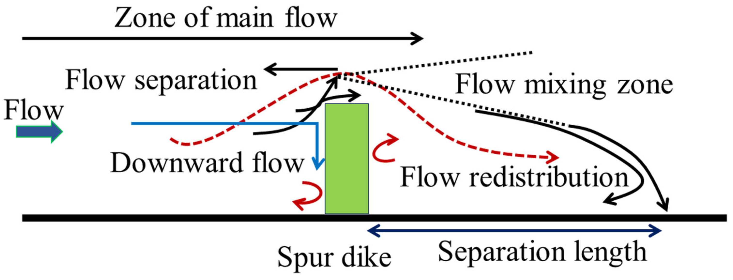
Furthermore, research has reported that scour depth induced by vortices provides critical insight into the complex behavior of flow, which directly contributes to scour development in the vicinity of the spur dikes. Within a channel, vortices of various types are generated as a result of flow interaction with spur dikes [3]. Figure 1 depicts the flow phenomenon around the spur dike. The flow separation and pressure gradient mechanism result in horseshoe vortices required for initiating sediment transport in the vicinity of the spur dike as reported by [13,14]. The sediment transport phenomenon increases through the recirculation zone, and wake vortices form at the downstream of the spur dike [15]. Flow interacting with the spur dike influences the geometrical change in the channel geometry and integrity of the spur dike because of non-uniform scour depth [5,6]. To optimize a spur dike for flood resilience, it is essential to understand the flow mechanism in the vicinity of the spur dike, which ultimately influences the hydraulic and structural efficacy of the dike.

Previously, researchers extended their approach for investigating flow dynamics and characteristics in the vicinity of the spur dike under different flow, hydraulic, and geometrical conditions utilizing computational fluid dynamics (CFD) [6,7]. Minimizing the construction cost and improving the environmental benefits of the spur dike, previously, researchers opted for selecting an optimal spacing between multiple spur dikes [16]. Studies have shown that selecting optimal spacing between multiple spur dikes significantly influences flow dynamics and erosive action in the vicinity of the spur dikes [5]. Therefore, it is essential to consider optimal spacing between spur dikes. If placed too near to one another, an upstream dike can shield the one immediately downstream, diminishing the flow velocities around it [17]. Conversely, if the spur dikes are too far apart, the collective system fails to protect the riverbank adequately [16]. Analytical models point to three major factors affecting threshold spacing: the Froude number (Fr), the ratio of channel width to dike length (B/b), and the ratio of channel width to water depth [18,19]. A limitation of past research is its heavy reliance on empirical data and evaluations of single parameters, which constrains how well the findings can be applied to a wide variety of flow conditions. The conventional approach of scour depth prediction and flow behavior depend on regression or empirical modeling, which often fail to capture nonlinear and complex patterns in the field of river engineering.

For this purpose, researchers have used advanced AI techniques to improve the prediction of various flow phenomena in rivers’ open channels under diverse scenarios [20,21,22,23]. Previously, researchers utilized advanced AI, including Random Forest (RF), Gradient Boosting Decision Tree (GBDT), Extreme Gradient Boosting (XGBoost), and neural network architecture to predict flow phenomenon and sediment erosion in the vicinity of the spur dikes with greater precision compared to traditional approaches [12]. Their findings recommended the superior performance of the RF and XGBoost models in predicting scour mechanisms around the spur dikes. Furthermore, three different advanced machine learning approaches were considered by Pandey et al. [24], who recommended the best predictive power of GBDT compared to other models. The superior performance of the XGBoost model was achieved with R² and RMSE values of 0.99 and 0.012 compared to the RF and neural network for predicting scour depth around the spur dike. A study conducted by Vaghefi et al. [20] utilized an experimental data series of a laboratory setting for training an ANN model for predicting velocity in a channel without and with a spur dike. The findings recommended that the ANN has strong predictive power with an R-value of 0.98, demonstrating its better performance in the prediction of flow velocity. According to Saber and Hassan [25], the AI model provides a more detailed assessment of flow interaction with the spur dike in terms of scour hole formation and the riverbank protection capability of a spur dike. The literature has widely reported the integration of advanced AI models in predicting flow dynamics, sediment erosion, and flow characteristics in the vicinity of spur dikes, enabling more precise, adaptive, and long-term sustainability of river systems [12,24].

Prior studies on the flow and scour patterns around spur dikes have widely used numerical and machine learning modeling to improve predictive precision. Introducing advanced machine learning models, including XGBoost, RF, and Gradient Boosting, signifies their greater accuracy in the prediction of temporal and maximum scour depths, indicating effectiveness in understanding nonlinear hydraulic flow–structure interaction as reported by [23,26]. The critical influence of various input parameters on scour depth was predicted using hybrid and ensembled machine learning techniques [27]. A FLOW-3D-based simulation was conducted using the RNG k-ε turbulence model to replicate laboratory-scaled scour dynamics, resulting in stronger agreement with experimental results [28]. Therefore, in the reported literature, it is evident that data-driven models have the capability of handling complex interactions while being effective in saving time, as computational/numerical modeling often takes longer to analyze such interactions. In the present study, advanced interpretable machine learning models were used to predict the tip velocity around a spur dike.

Conventional techniques, such as regression-based and empirical models, cannot capture a complex and nonlinear relationship between flow-induced variation around the spur dike under diverse hydraulic and geometrical scenarios. However, it is essential to optimize spur dike design for analyzing its critical role in flow regulation, sediment transport, and stabilization of the riverbank. Therefore, in the vicinity of a spur dike, precise prediction of the flow dynamics remains a challenge in the field of river engineering. Numerous studies have been conducted to evaluate turbulence characteristics, flow dynamics, and scour around the spur dike using numerical and experimental methods. However, the prediction of tip velocity around the spur dike utilizing advanced interpretable machine learning and SHAP analysis is underexplored.

Furthermore, prior studies have the prediction of scour depth and the flow field around the spur dike using traditional empirical equations or regression models, which have limited ability to capture the complex hydraulic interactions. Prior research has not considered the relative importance of hydraulic and geometric parameters. Therefore, the present study fills this gap by introducing four advanced interpretable machine learning models, namely GPR, CatBoost, RF, and XGBoost–PSO, for predicting tip velocity around the spur dike. Moreover, the contribution of input parameters was quantified using SHAP analysis to understand flow–structure interactions. This research offers a novel and comprehensive framework that integrates predictive model performance with interpretability across diverse geometric and hydraulic scenarios, particularly when limited laboratory-scale data points are available. The main objectives of the current research are the following: (1) to understand the relationship between input and output variables using a correlation heatmap, (2) to compare and analyze the predictive capability of different AI models using performance metrics, and (3) to analyze the influence of input parameters on the predicted values of tip velocity utilizing SHAP analysis.

2. Methodology

2.1. Experimental Setup and Data Collection

In this study, data points were collected from a study conducted by Yeo et al. [29] in a channel with a length of 40 m, a width of 2 m, and a height of 0.65 m. A discharge of 0.012 to 0.4 m³/s was supplied from the storage tank and measured through a weir of 1.2 m installed in a channel. This laboratory setup was utilized to measure the tip velocity of spur dikes of varying permeability and geometrical conditions. For this purpose, a spur dike was modified by introducing porosity ranging from 0 to 60% and varying l/B (where l: length of spur dike and B: channel width). Tip velocity in a controlled laboratory setting was measured through advanced tools like an Acoustic Doppler Velocimeter (ADV) with a 25 Hz frequency manufactured by Nortek AS. Yeo et al. [30] used ADV for tip velocity measurement because of its ability to measure three-dimensional velocity around the spur dike at 60% water depth. Parameters such as tip velocity and velocity field were measured at a time interval of one minute. However, the velocity field in a channel was computed using CACTUS 3.1. CACTUS 3.1 is a computer-aided calculation for the Time-averaged Underlaying Shear tool that uses the ADV data to calculate the velocity field, developed by Nortek. For investigating the recirculation zone in the vicinity of the spur dike, the LSPIV technique with a digital video camera (DTR-TRV900, Sony Co., Tokyo, Japan) was adopted. LSPIV denotes Large-Scale Particle Image Velocimetry, used to evaluate the pattern of surface velocity by tracking the moment of particles. Yeo et al. [29] implemented LSPIV using a Sony digital tape camcorder (DCR-TRV900) to quantify recirculation zones of flow near the spur dike. Appendix A summarizes the range of experimental and hydraulic parameters considered in an experimental study conducted by Yeo et al. [29].

In this study, a data series was collected from the published literature, where parameters like spur dike length (l), channel width (B), separation length (L), incidence angle (β), and Froude number (Fr) were considered. Previous studies focused on the non-dimensional parameters for developing AI models [30,31]. Therefore, in the current research, three input parameters, including Fr, L/l, β, and tip velocity, were considered as output parameters. These parameters were selected considering their influence on the flow behavior around the spur dike. A total of 69 data points were chosen for developing AI models. Before developing an AI model, a correlation heatmap and the relationship between input and output parameters were assessed. Based on the selected data points, this study used four advanced AI models: Random Forest (RF), Categorical Boosting (CatBoost), Extreme Gradient Boosting (XGBoost) with Particle Swarm Optimization (PSO), and Gaussian Process Regression (GPR). The selected models have the capability of avoiding the risk of overfitting, which may be an issue for such a small data series. Therefore, these four models provide a reliable and accurate prediction of the tip velocity of the spur dike. Once the data series and models were considered, this study assigned the data series into three different phases. The three phases considered in this study were training, testing, and validation, for which 70%, 15%, and 15% of the data were assigned, as adopted by [32,33].

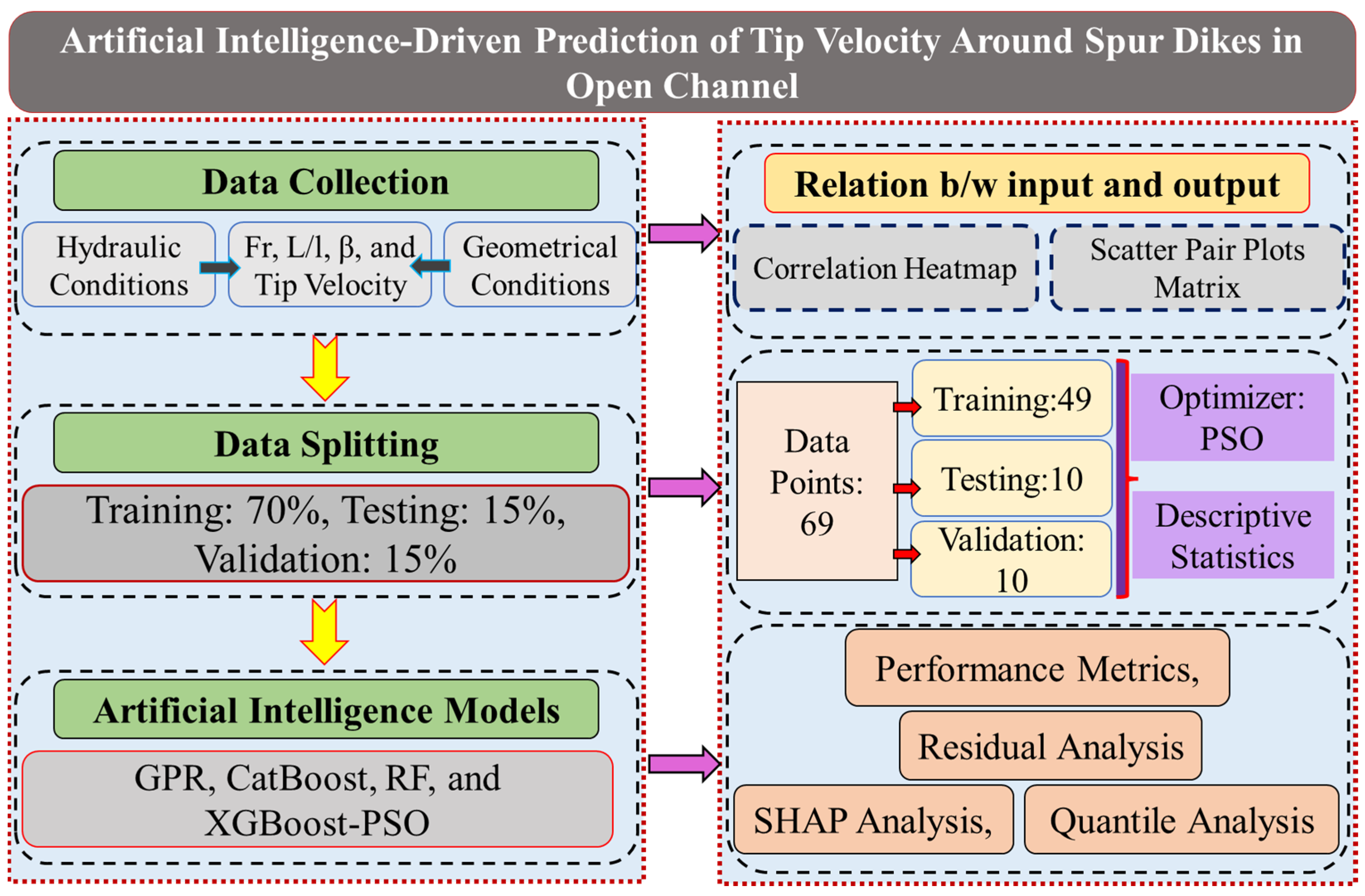
Although this study used minor data points consisting of 69 samples, it reflects the complex interaction of flow structures. However, advanced machine learning such as RF, CatBoost, XGBoost–PSO, and GPR as reported in the previous research have demonstrated superior performance in modeling nonlinear relationships between limited data points [34,35,36]. Algorithms such as Random Forest and Gradient Boosting reduce overfitting through ensemble learning, while Gaussian Process Regression provides probabilistic predictions with uncertainty estimates. In addition, model complexity was controlled through regularization and hyperparameter optimization to mitigate overfitting risks. The small amount of data available creates uncertainty in terms of sampling variability and possible overfitting of the model. Even though cross-validation enhances the strength, results can only be seen as its trends and not an absolute forecast. Gaussian Process Regression is one of the models that gives probabilistic results, which offers the opportunity to estimate the probability limits. More studies on future research ought to use larger sample sizes across several locations to enhance predictive reliability. For evaluating the performance of these AI models, different metrics, including the coefficient of determination (R²) and root mean square error (RMSE), were calculated. Further, to assess the contribution of each parameter to the tip velocity around the spur dike, SHAP analysis was performed. Furthermore, quantile and residual analyses were performed to evaluate the difference between the actual and predicted values of the tip velocity. Figure 2 shows the flowchart of the methodology adopted in this study. The details of selected descriptive statistics, AI models, SHAP analysis, and performance metrics are presented in the subsequent sections.

2.2. Descriptive Statistics

In this study, a descriptive statistics analysis was performed as summarized in

Table 1. Summary of descriptive statistics performed in this study for the collected data points.

Parameter	Mean	Mode	Standard Deviation	Variance	Range	95% CI Lower	95% CI Upper
L/l	6.05	0.00	5.19	26.89	12.50	4.80	7.29
Fr	0.27	0.25	0.05	0.00	0.15	0.25	0.28
β°	7.80	0.00	10.29	105.85	45.00	5.32	10.27
Tip Velocity	0.43	0.31	0.14	0.02	0.65	0.40	0.46

. The obtained descriptive statistics show a comprehensive analysis of the data series collected from the experimental setup, demonstrating the variability and central tendencies of the parameters. The descriptive statistics results are explained in this section concerning the parameters collected. For instance, the ratio L/l has a broader range of 12.50, a mean value of 6.05, a standard deviation of 5.19, and at a 95% confidence interval, the variability was between 4.80 and 7.29, indicating the diverse nature of the structural configuration datasets. In the case of Froude number (Fr), the descriptive statistics show more consistent behavior compared to L/l because the mean, range, and standard deviation values were 0.27, 0.15, and 0.05, respectively. Further, a flow regime was controlled in an experimental study conducted by Yeo et al. [28], as confirmed by the 95% confidence interval (variability 0.25 to 0.28). Meanwhile, in the case of incidence angle (β°), the data series show greater dispersion with a range, mean, and standard deviation of 45°, 7.80°, and 10.29°, respectively. However, the descriptive statistics confirmed the inclusion of both steep and mild scenarios of spur dikes located in a channel. This confirms the diverse nature of the flow interaction with the spur dike. The variability reported at a confidence interval of 95% indicates values between 5.32 to 10.27, demonstrating that the incidence angle ranged within the lower limit, demonstrating greater deflection of flow interacting with the spur dikes. The descriptive statistics of the predicted/targeted variable (tip velocity) have mean, range, and standard deviation values of 0.43 m/s, 0.65 m/s, and 0.14 m/s. In contrast, the variability (0.40 to 0.60 m/s) reported at the confidence interval of 95% confirmed the accuracy of ADV and LSPIV in measuring tip velocity with greater reliability and lower impact of outliers. The descriptive statistics analysis indicates diversity in the structural configuration of the spur dikes. At the same time, stability and reliability of the flow regimes, including Fr and tip velocity, provide a balanced set of data points for further modeling and analysis.

2.3. Artificial Intelligence

2.3.1. Extreme Gradient Boosting (XGBoost) with PSO Model

For predicting tip velocity of the spur dike located in an open channel, in the current study, an Extreme Gradient Boosting (XGBoost) model was adopted by considering the Froude number (Fr), ratio of separation length (L) to spur dike length (l), L/l, and angle of incidence (β°) as input parameters, while the output parameter was tip velocity. Before assigning a dataset to the XGBoost model, it was cleaned and pre-processed, followed by division into three different phases, including training (70%), testing (15%), and validation (15%), to ensure that an assessment could be made based on unseen data series. Extreme Gradient Boosting (XGBoost) is an advanced artificial intelligence model working based on the ensemble learning trees, which builds successive trees, where each tree corrects the error made by the previous trees. The predictive power of the XGBoost model is greatly influenced by hyperparameters such as the learning rate, the number of estimators, and the maximum tree depth. To avoid such issues, in this study, a particle swarm optimization (PSO) was employed to enhance the process. The purpose of introducing PSO was to reduce the value of mean squared error (MSE) in the test data series. For the identification of optimal arrangement, each parameter was assigned specific boundaries so that the PSO algorithm searched for the parameter space using iterations. After the identification of the optimal hyperparameters, the model was trained again, utilizing datasets assigned to the training and testing phases. This methodology adopted for the XGBoost model provides the predicted values of the tip velocity around the spur dike, and the performance was assessed in terms of R² and RMSE.

In this paper, the XGBoost model uses an additive tree-based model for gradient boosting. The second-order Taylor approximation of the loss function was minimized by training each new regression tree with the following model structure.

$$\widehat{y_i}={\displaystyle \sum }_{k=1}^K{f}_k\left(x_i\right), f_kϵ \mathrm{F}$$

(1)

In the above Equation (1), $\widehat{y_i}$: predicted value of the tip velocity at the ith data point; k: total number of trees used in the model; $x_i$: value of input parameter at the ith data point; k: index of tree number; F: space of all possible regression trees; $f_k$: kth function.

The Particle Swamp Optimization (PSO) was used to optimize key hyperparameters, including maximum tree depth, learning rate, and the number of estimators. Individual and global best solutions are used to update the individual and global position.

$${\mathrm{v}}_{\mathrm{i}}^{\mathrm{t}+1}={\mathrm{wv}}_{\mathrm{i}}^{\mathrm{t}}+{\mathrm{c}}_1{\mathrm{r}}_1\left({\mathrm{p}}_{\mathrm{i}}-{\mathrm{x}}_{\mathrm{i}}^{\mathrm{t}}\right)+{\mathrm{c}}_2{\mathrm{r}}_2\left(\mathrm{g}-{\mathrm{x}}_{\mathrm{i}}^{\mathrm{t}}\right)$$

(2)

In Equation (2), ${\mathrm{v}}_{\mathrm{i}}^{\mathrm{t}}$: velocity at iteration t of particle I; ${\mathrm{v}}_{\mathrm{i}}^{\mathrm{t}+1}$: updated velocity particle I; w: inertia weight controlling exploration; c₁, c₂: cognitive and social learning factor; r₁, r₂: random value in (0, 1); p_i, g: best solution by particle i and entire system; ${\mathrm{x}}_{\mathrm{i}}^{\mathrm{t}}$: particle i position at iteration t; t: number of iterations. Mean Squared Error (MSE) worked as an objective function during the validation phase. Therefore, an XGBoost–PSO framework enhances generalization by convergence behavior and automatically regulates the model’s complex nature.

2.3.2. Random Forest (RF) Model

In this study for predicting the tip velocity around the spur dike, a Random Forest (RF) model was used because of its ability to precisely predict the hydraulic and hydrodynamic phenomenon around the structures. Previous research reported that the RF model is the most reliable AI approach, comprising multiple trees and capable of predicting different phenomena [37]. The RF model worked under the mechanism of combining the predictions of multiple trees, out of which the average value of the prediction was considered to avoid the issue of overfitting and generalization enhancement. For developing an RF model, in this study, similar input and output parameters were considered as adopted in the XGBoost–PSO model. In the current paper, the utilized RF consisted of 200 trees as an estimator with a maximum depth of 10 to enable the model to balance the computational efficacy and nonlinearity. In the training, testing, and validation phase of the RF model, a data series of 70%, 15%, and 15% was assigned so that the model could learn the association between hydraulic and geometrical parameters used in this study, influencing tip velocity in the vicinity of the spur dike. The performance of the model was assessed considering its performance metrics after the training phase, explaining how the RF model shows the variance between actual and predicted values of the tip velocity.

An ensemble learning algorithm such as a Random Forest model, consists of several independent decision trees adopting random feature selection and bootstrapped samples. The predicted value of the tip velocity was obtained through ensemble averaging using Equation (3).

$$\widehat{{\mathrm{y}}_{\mathrm{i}}}={\displaystyle \frac{1}{\mathrm{N}}}{\displaystyle \sum }_{\mathrm{j}=1}^{\mathrm{N}}{\mathrm{T}}_{\mathrm{j}}\left(\mathrm{x}\right),$$

(3)

In Equation (3), N: total number of trees; T_j: prediction from the jth decision tree; j: index of tree. The variance of the model was minimized using randomness at both feature and data levels. To avoid the overfitting issue and impurity measure, the tree depth was constrained based on the Mean Squared Error. The RF model was selected considering its realistic approach in the development of the relationship between input and output parameters without needing previous assumptions, making it a greater choice for problems in the field of hydraulic engineering, such as the flow field in the vicinity of the spur dike.

2.3.3. Categorical Boosting (CatBoost) Model

CatBoost is a decision tree-based gradient boosting algorithm that introduces innovations to effectively handle categorical data, minimize overfitting, and perform much faster computations. This study used a CatBoost with 500 iterations, a learning rate of 0.1, and a tree depth of 6. These hyperparameters were selected to be able to balance the complexity of learning and computational cost in such a way that the model would be able to incorporate the complex interaction between input parameters and at the same time avoid unnecessary overfitting. The data were pre-processed before the development of the model to remove inconsistencies and make sure that the predictor and response variables were aligned appropriately. In the case of datasets with a wide range of numerical values, standardization was used for feature scaling because CatBoost optimizes with normalized input values. This pre-processing procedure ensured that all the parameters contributed at the same level to the learning process. The training model was then trained in the scaled dataset, and its predictions were then optimized by targeting the errors recorded in earlier training. Following training, CatBoost was used to forecast the values of the tip velocity of the dataset. The CatBoost model was developed using 70%, 15%, and 15% of the data for training, testing, and validation, respectively. For assessing the performance of the CatBoost model, R² and MSE values were used. The variation in the predicted and observed values of tip velocity was assessed based on R², and the average error between observed and predicted values of the tip velocity was assessed using MSE values. The prediction capability of the CatBoost model was assessed using the above-mentioned steps.

CatBoost consists of a gradient boosting algorithm that uses a symmetric tree structure and an ordered learning process to enhance training stability and minimize bias. CatBoost does not maximize the shift in predictions like traditional methods of boosting, and instead, its internal regularization structure helps reduce prediction shift. The other model parameters, including the learning rate, number of iterations, and the number of tree depths, were adjusted to trade off between learning speed and model complexity. The feature scaling was used to create consistency between input variables. CatBoost is also suitable, especially with small datasets, because it possesses high generalization properties and avoidance of overfitting. The effectiveness of the CatBoost model in evaluating the hydraulic and computational approaches makes it suitable in this study, where it can predict output besides the complex and nonlinear relationship among parameters. The diverse nature of the data series collected from the laboratory experiments also makes it suitable for predicting tip velocity in the vicinity of the spur dike.

2.3.4. Gaussian Process Regression (GPR) Model

A GPR model was adopted as a nonparametric and probabilistic prediction framework to determine the tip velocity near spur dikes. The pre-processing involved cleaning the column names so that they remained consistent and scaling the features in the input by standardization. Gaussian Process Regression was used, in which a radial basis function kernel is multiplied by a constant kernel to estimate the nonlinear association between input variables and tip velocity. Before training, the feature variables were first standardized with a StandardScaler to enhance the numerical stability and efficiency of the kernel. The model was also able to optimize the kernel parameters using marginal likelihood with ten restarts of the optimizer to ensure that it did not converge to the local optima. The coefficient of determination and mean squared error were used to estimate the model’s performance. Feature scaling was a critical stage since GPR is very sensitive to variations in the magnitudes of input features; feature normalization enabled the comparison of each variable on a similar scale using the kernel-based approach. GPR works based on the assumption that data may be modeled as a sample of a multivariate Gaussian distribution, and a kernel function models the covariance structure. The Radial Basis Function (RBF) kernel was used in this paper, and a constant kernel was used to gain flexibility to capture smooth variations and broader trends in the dataset. The algorithm itself performed an internal search based on multiple restarts to optimize the kernel hyperparameters in order to maximize the likelihood and soon arrived at an appropriate solution to the initially given dataset. The standardized dataset was passed through the model to make predictions on all the samples as well. The initial 53 predicted values were removed, and the observed tip velocities were compared to the predicted ones to avoid any inconsistency in the models. R² and MSE were used in determining model performance. R² was used to give insights into what percentage of the predicted variable variance was observed, and the MSE measure was used to gauge the occurrence of an average error in prediction among the variables. The combination of these measures proved the validity and predictability of the model. The GPR methodology turned out to be especially beneficial since the given methodology did not just predict the points but had the inherent element of modeling the uncertainty of the predictions made. Such a more probable character often comes into practice in hydraulic engineering issues, where variability of measurements and uncertainties of experiments are typical. With a well-integrated robust kernel function and a probabilistic framework, GPR proved to be a potent and flexible tool when predicting tip velocity in spur dike flows and an enhancement of ensemble-based methods.

2.4. Model Development

In this study, four different AI models, namely GPR, CatBoost, RF, and XGBoost–PSO, were used to predict tip velocity in the vicinity of the spur dike under the diverse geometrical and hydraulic conditions summarized in

Table 2. Development of four AI model used in this study.

Configuration Item	XGBoost (XGBoost–PSO)	Random Forest (RF)	CatBoost	GPR
Algorithm family	Gradient boosting trees (XGBoost)	Ensemble of decision trees (bagging)	Gradient boosting trees (CatBoost)	Kernel-based probabilistic regression
Input features	`L/l`, `Fr`, `β°`	`L/l`, `Fr`, `β°`	`L/l`, `Fr`, `β°` (scaled)	`L/l`, `Fr`, `β°` (scaled)
Target	Tip Velocity	Tip Velocity	Tip Velocity	Tip Velocity
Data split	Train/Test/Valid split (70/15/15)	Train/Test/Valid split (70/15/15)	Train/Test/Valid split (70/15/15)	Train/Test/Valid split (70/15/15)
Feature scaling	No scaling in code	No scaling in code	`StandardScaler()` applied	`StandardScaler()` applied
Key hyperparameters	`max_depth`, `learning_rate`, `n_estimators`—optimized by PSO	`n_estimators = 200`, `max_depth = 10`	`iterations = 500`, `learning_rate = 0.1`, `depth = 6`	Kernel: C (1.0) RBF (length_scale = 1.0); n_restarts_optimizer = 10
Hyperparameter optimization method	PSO optimizing MSE on test set; bounds: max_depth [2–10], learning_rate [0.01–0.3], n_estimators (50–300); swarmsize = 10, maxiter = 5	No algorithmic tuning in code	No tuning (preset values used)	Hyperparameters optimized by log-marginal likelihood
Objective/loss used for tuning and training	Regression: reg:squarederror (minimize MSE)	Mean squared error minimization	Gradient boosting regression loss (MSE)	Maximizes log-marginal likelihood; predictions include uncertainty
Training procedure notes	PSO loop trains candidate models; final retrained with best params	Trained on X_train, predicts 53-sample test set	Model trained on scaled X, first 53 predictions used	Trained on scaled X; predictions made for all samples
Evaluation metrics reported	R2, Mean Squared Error (MSE)	R2, MSE (prints predictions count = 53)	R2 (first 53), MSE (first 53)	R2 and MSE
Random seed/reproducibility	train_test_split(random_state = 42); no explicit PSO seed	random_state = 42 for reproducibility	random_seed = 42` used for reproducibility	Deterministic, n_restarts_optimizer = 10 to avoid local optima
Practical remarks	PSO adds compute overhead but automates tuning	Balanced configuration with fixed test set for fair comparison	Strong fitting capacity: scaling helps stability	Provides predictive variance; best for smaller datasets

. For instance, the XGBoost–PSO model was utilized to tune the hyperparameters for the required result (

Table 3. Hyperparameter settings used for each machine learning model.

Model	Hyperparameter	Value
XGBoost–PSO	Booster	Gradient Boosted Trees
	Objective Function	reg:squarederror
	max_depth	Optimized (2–10)
	learning_rate	Optimized (0.01–0.30)
	n_estimators	Optimized (50–300)
	Optimization Method	Particle Swarm Optimization (PSO)
	PSO Swarm Size	10
	PSO Iterations	5
	Fitness Function	Mean Squared Error (MSE)
Random Forest	n_estimators	200
	max_depth	10
	Split Criterion	Mean Squared Error
Gaussian Process Regression	Kernel	C (1.0) × RBF (length_scale = 1.0)
	Optimizer Restarts	10
	Input Scaling	StandardScaler
	Prediction Type	Probabilistic
CatBoost Regressor	Iterations	500
	Learning Rate	0.10
	Tree Depth	6
	Loss Function	RMSE
	Feature Scaling	StandardScaler

). During optimization of the XGBoost with PSO, the following were used to reduce the difference between observed and predicted values of the tip velocity: (1) estimator = 50 to 300, maximum tree depth = 2 to 10, and learning rate = 0.01 to 3. The factors utilized for the development of the XGBoost–PSO enhanced the prediction and generalization through the best parameters. Furthermore, the RF model used in this study has a maximum tree depth of 10, and the number of decision trees was 200. The number of decision trees and maximum tree depth utilized for the RF improved the performance of the model and captured a precise relationship between input and output parameters. By obtaining predictions from different decision trees, RF avoids the issue of overfitting.

The learning rate of 0.1 and tree depth of 6 were used to train the CatBoost model (500 iterations), which is a reasonable trade-off between learning capacity and training stability. Before training the models, they were scaled in terms of features so that L/l, Fr, and β° were all treated evenly. The CatBoost gradient boosting system gradually improved its prediction whilst being resistant to overfitting; therefore, it was able to fit the more challenging nonlinear dependencies. In the case of the Gaussian Process Regression (GPR) model, the optimization was based on the choice of the kernel. A composite kernel (that is, a combination of a constant kernel and a Radial Basis Function, RBF) was used to persist both longer-term trends of the data and local smoothness. Numerical stability was obtained with the means of standardization of inputs, and the maximization of hyperparameters was made possible by the repeated likelihood maximization procedure with numerous restarts. This scheme gave precise predictions as well as quantitative uncertainty, which is a clear advantage compared to the traditional ensemble methods. The selected configurations adapted each model to what suited it best to allow a sound comparison to see between machine learning methods in predicting tip velocity around spur dikes.

3. Result and Discussion

3.1. Correlation Heatmap

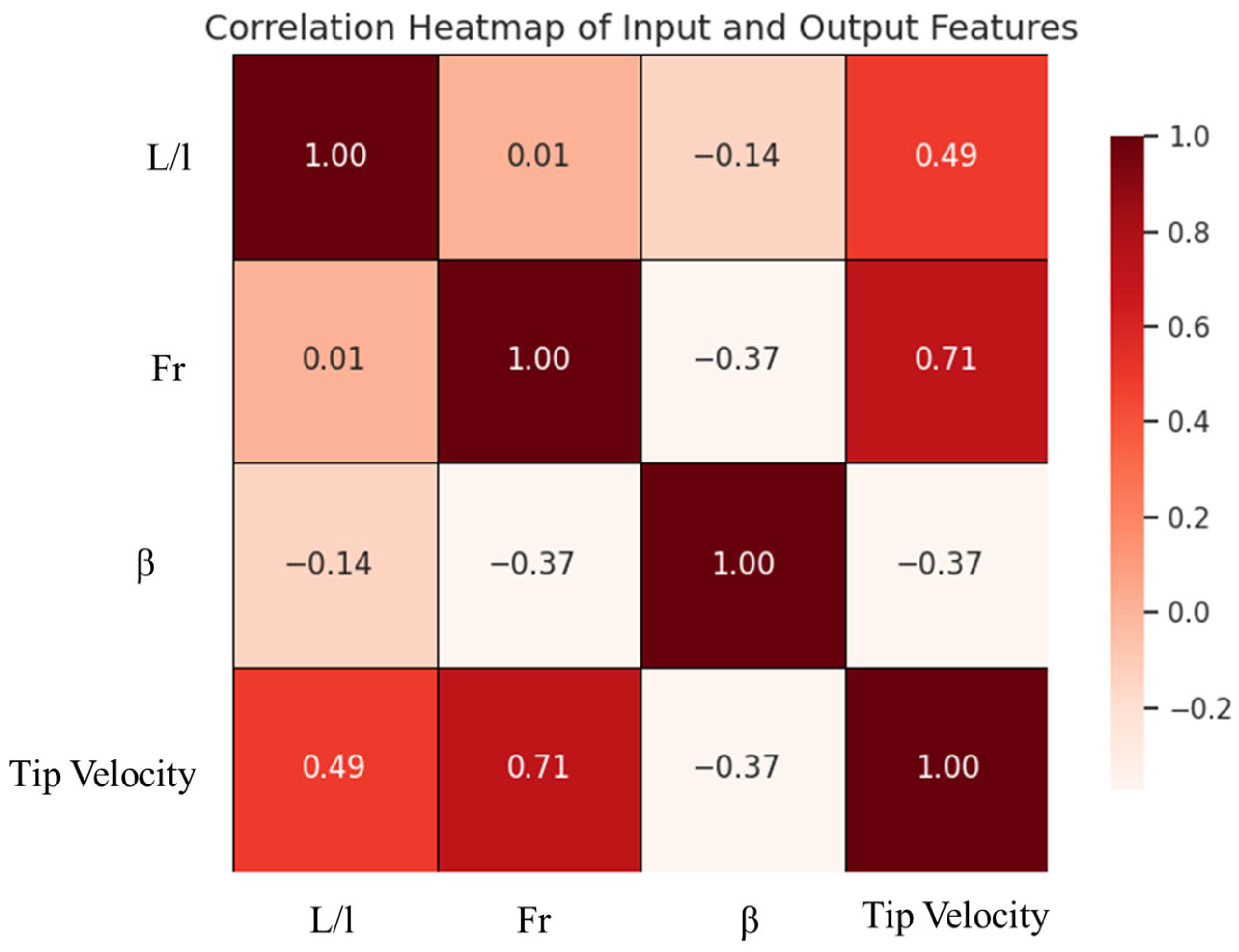
In this paper, the correlation heatmap gives a critical insight into the relationship between separation length ratio (L/l), Froude number (Fr), incidence angle (β°), and tip velocity in the vicinity of the spur dike. The result of the correlation heatmap for input and output parameters utilized in this study is presented in Figure 3. Figure 4 depicts the result of both hydraulic and geometrical parameters on the tip velocity in the vicinity of the spur dike. In this study, a correlation heatmap is presented to show the relationships between three input and one output parameters, which are explained below. Out of the tested input parameters, the correlation heatmap shown in Figure 3 demonstrates a greater influence of the Fr on the tip velocity with a correlation coefficient (R) value of 0.71, aligning with the previously reported results in the literature [38,39].

Furthermore, Vaghefi et al. [40] and Jeon et al. [41] concluded that there is a direct relationship between tip velocity and flow regimes (Fr). The greater influence of Fr on the tip velocity indicated higher variation in the distribution of turbulence and magnitude of velocity around the spur dike. Researchers investigated excessive scour depth around the spur dike under extreme flow regimes, where flow interacts with the spur dike at greater flow velocity, initiating sediment transport [42]. In the case of observing the relationship between tip velocity and (L/l), an R-value of 0.49 was demonstrated, indicating a greater impact of L/l on the tip velocity in the vicinity of the spur dike. A study conducted by Kang et al. [43] and Ho et al. [44] concluded that dike geometrical orientation greatly influenced flow turbulence and redistribution around the spur dikes.

The result of this work demonstrated that intense tip velocity of the spur dike resulted in the generation of separation length, recirculation zones, and velocity gradient on the spur dike tip; thus, the risk of erosion increased around the spur dike. Furthermore, in this study, the influence of the incidence angle (β°) demonstrated a negative correlation with tip velocity, with an R-value of −0.37 as shown in Figure 4. The value of tip velocity was reduced, and flow deflection was enhanced around the spur dike by increasing the incidence angle of the spur dike, which aligns with the result of the study conducted by Li et al. [45] and Jafari and Sui [38]. Studies presented in the literature also investigated the minimization of tip velocity, local turbulence, and hydrodynamic mechanisms around the spur dike by the optimization of incidence angle, which alternately enhanced the habitats of aquatic life and riverbank protection [38,45]. This research recommended that sediment transport pathways and channel geometry (widening of the channel) were significantly altered by increasing the value of the spur dike incidence angle. Furthermore, it is recommended that when designing a spur dike for reducing tip velocity, the hydraulic and geometrical conditions of the spur dike should be considered. Therefore, the potential risk of scour and flow dynamics can be balanced by the optimized geometry and hydraulic conditions of the spur dike.

3.2. Scatter Pair Plots

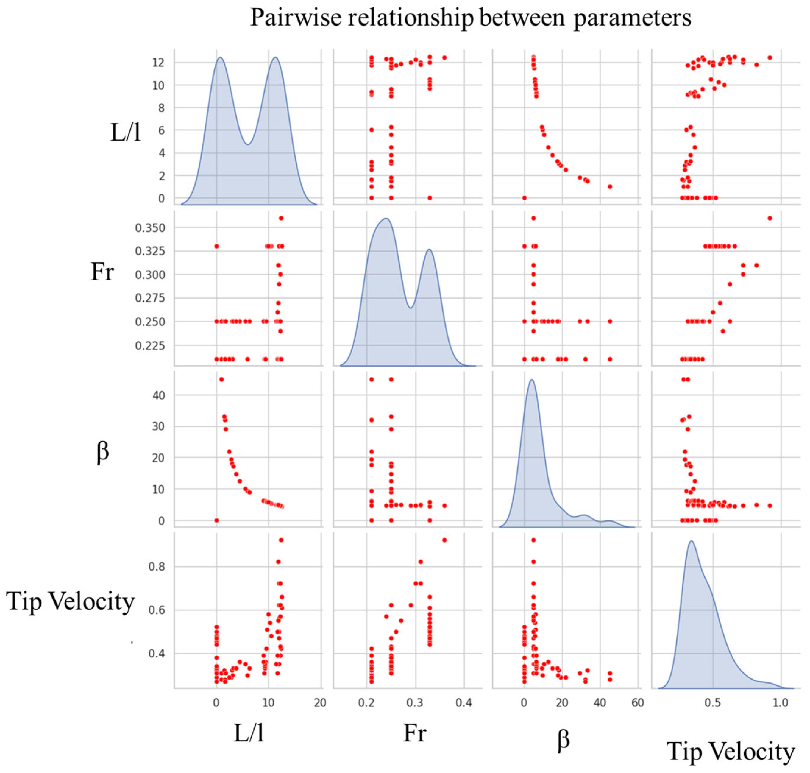
In this paper, a scatter pairwise plot was drawn to observe the relationship between Fr, L/l, β, and tip velocity, as shown in Figure 4. The result in this section is explained considering the kernel density estimate and histogram for each input parameter. The distribution reported for L/l demonstrates bimodal variation, demonstrating the geometrical and flow regimes of the spur dike utilized in this study. In the case of β, most of the tip velocity values clustered around 0.40 and 0.60, demonstrating a positively skewed and unimodal distribution for numerous data points at lower values of the incidence angle (β). The values of L/l and β show an inverse relationship, demonstrating the increasing ratio of flow separation length and spur dike length due to lower incidence angle values. This means that under a lower-value incidence angle, greater flow separation zones are created in the vicinity of spur dikes compared to a higher-value incidence angle. Following the relationship between L/l and β, the value of incidence angle shows a clustered relationship with Fr, indicating that under lower values of β, the flow approaches the spur dike with greater inertial forces compared to higher values of β.

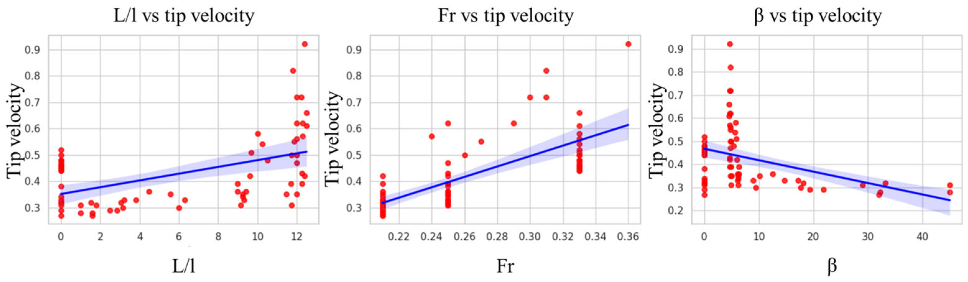
The most vital relationship is that between the input parameters and the output, tip velocity. Based on the scatter plots, the tip velocity is dependent on L/l and Fr. An increased L/l ratio typically signifies more flow impediment by the spur dike, resulting in increased speed of flow around the dike tip. Likewise, with an increase in Fr, inertial forces have the dominant effect over gravitational forces, and the flow constricts more at the tip, producing greater tip velocities. On the other hand, the correlation between β and tip velocity is inversely related. At lower β values, the velocity at the tip is greater so that as the flow hits the spur dike at a smaller angle, it creates a stronger jet around the tip. These results have significant hydraulic consequences. Such high tip velocities have been shown to promote local scour potential at the spur dikes, which is a determinant in the design of river-training works and bank protection. According to the analysis, it might be possible to enhance the tip velocities by reducing the L/l ratio or by developing with larger incidence angles, but this would conflict with the existing goals of reducing flow conveyance and sediment management. Also, in rivers with fluctuating discharge, manipulation of flows to decrease scour risk may be required, as Fr is highly sensitive to the velocity of the tip.

Furthermore, to confirm the relationship between the input (L/l, Fr, and β) and output (tip velocity) parameters, a regression plot was drawn for clear visualization purposes as shown in Figure 5. The regression plots demonstrate how input parameters influence the output parameter. This can be attributed to the increased contribution of flow contraction and acceleration around the tip of the dike in the cases where the structure is longer in comparison to the separation zone. The second plot (Fr vs. tip velocity) shows that the linear relationship is strong and positive. Greater Froude numbers (i.e., inertial forces as compared to gravity) substantially enhance tip velocity. This indicates that the flow regime is the major cause of scouring potential around the dike since the greater the depth, the higher the erosive energy. On the contrary, the third plot (β versus tip velocity) exhibits an inverse relationship. At steeper angles of incidence, the velocity of the tip is increased, with the approaching flow actually striking directly to the dike and thus producing energy close to the tip.

3.3. Five-Fold Cross-Validation

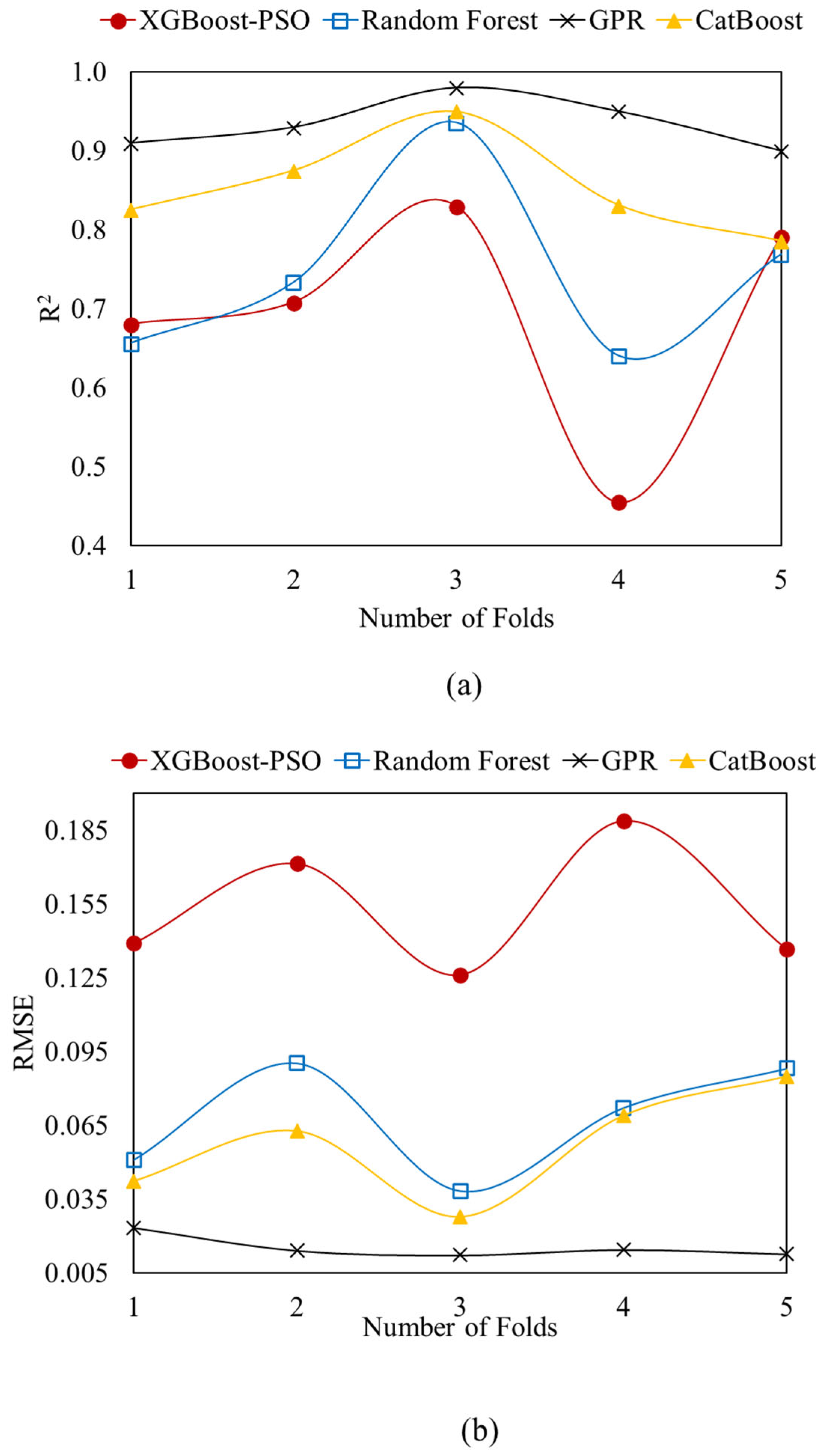
In this study, the robustness of each model was assessed using 5-fold cross-validation, highlighting comparative performance and generalization of the four tested advanced interpretable machine learning models, as shown in Figure 6. Out of the tested models, GPR demonstrated superior performance in terms of accuracy and prediction of tip velocity, with R² and RMSE values of 0.98 and 0.012 in fold number 3, respectively. However, the greater average R² value of 0.934 and the lowest RMSE value of 0.015 demonstrate strong predictive capability across all folds to capture complex relationships in a small number of data points and minimal prediction error. Therefore, the findings of GPR from the 5-fold cross-validation suggest the suitability of this model for smaller to medium-sized data points. Furthermore, in the case of the CatBoost model, the highest value of R² and the lowest value of RMSE achieved were 0.95 and 0.027 across fold number 3. However, the average highest R² and lowest RMSE reported from all five folds were 0.856 and 0.057, indicating stable performance. The relatively higher prediction error across folds 1, 2, and 5 and lower variance in folds 3 and 4 demonstrate its capability for handling nonlinear interaction between input and output parameters.

Random Forest was also fairly well-performing, offering an average R² of 0.747 and an RMSE of 0.068, which is a good predictive power but with a somewhat larger variation and error than CatBoost and GPR. It is possible to note that the performance pattern across folds suggests that the Random Forest can model nonlinearity but is likely to be sensitive to data distribution across splits when bootstrapping aggregation is used with limited datasets. Contrastingly, the XGBoost–PSO represents the lowest results when compared to the other three options: It has an average value of R² = 0.693 and RMSE = 0.151, meaning that XGBoost–PSO has quite high prediction error and lacks relative consistency in cross-folds. Although XGBoost can be considered strong, the tuning of hyperparameters provided by PSO might have been limited by the small sample size of the dataset and resulted in suboptimal generalization. The broader variation in both R² and RMSE between folds is also an indication of sensitivity to fold-wise changes in the data.

The comparison indicates that the model behavior is considerably different between the datasets of different sizes, distribution of features, and the structure of algorithms, with GPR and CatBoost demonstrating better generalization, Random Forest with moderately good results, and XGBoost–PSO that will have to be tuned or trained on a larger scale. Those findings highlight the significance of the choice of algorithms depending on the data properties: smooth models of probabilities like GPR perform better with small datasets, whereas ensemble and boosting algorithms may need richer distributions of data to be at their best.

3.4. Performance Metrics

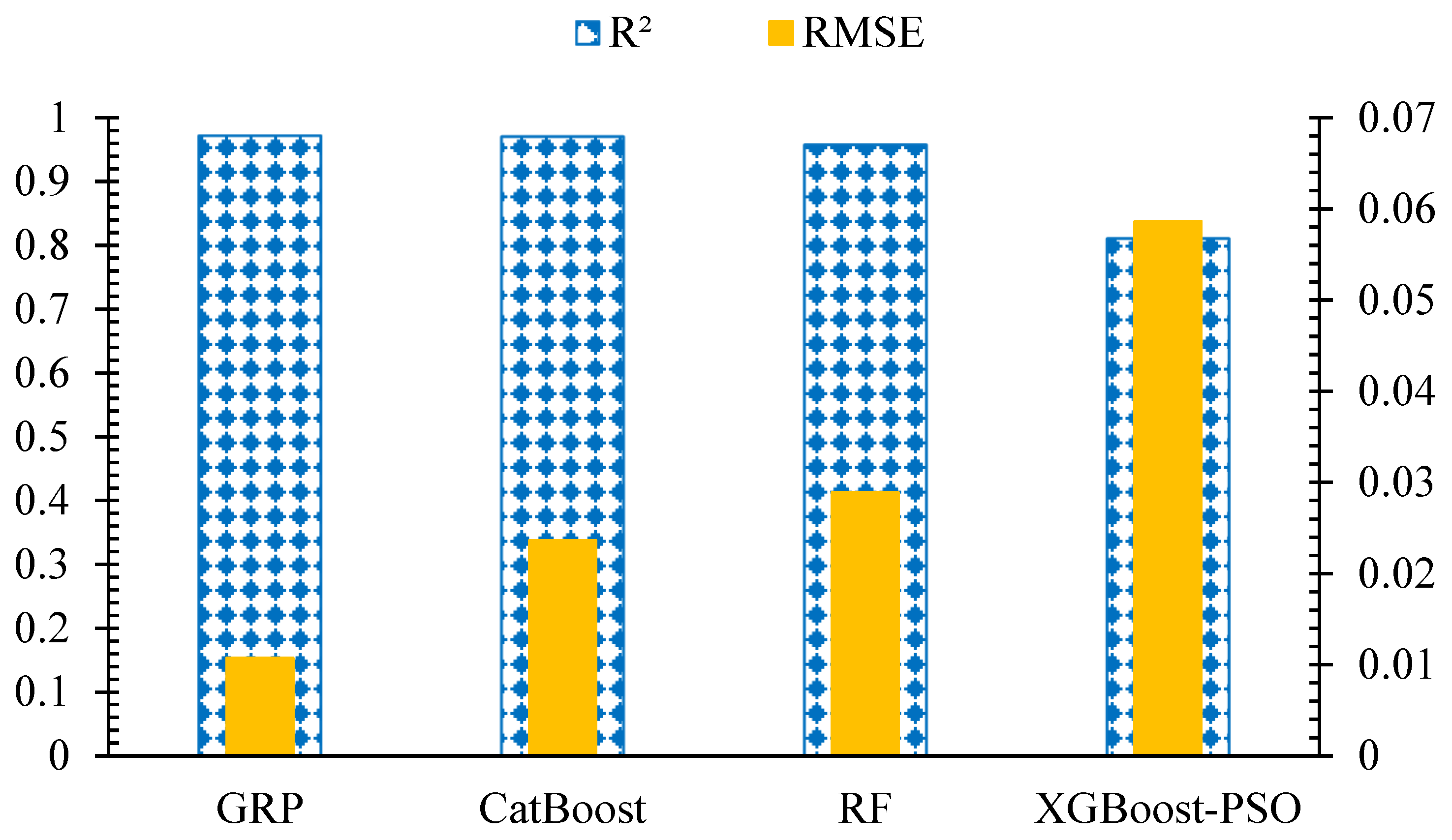
In this section, a detailed assessment of the performance metrics of AI models utilized in this study is provided. The performance metric includes the Coefficient of Determination (R²) and Root Mean Square Error (RMSE), providing critical feedback on the predictive power of the utilized models in predicting tip velocity in the vicinity of the spur dike. Out of the four tested AI models, the performance metrics, such as higher R² and RMSE values of 0.972 and 0.0107, demonstrated the superior performance of the GPR, making it a more reliable approach in predicting tip velocity in the vicinity of the spur dike, as shown in Figure 7. Following the GPR model, the CatBoost model has much closer values of R² (0.9704) and RMSE (0.0236) to the GPR model. However, out of these two models, the lower RMSE value of GPR indicates superior performance compared to CatBoost, with a higher RMSE value. Further, the RF model also provides a prediction of tip velocity with R² and RMSE values of 0.9575 and 0.0289. This highlights that the RF model can handle a nonlinear relationship between input parameters and tip velocity in the vicinity of the spur dike. In contrast, the XGBoost–PSO model demonstrates weaker performance compared to the other three models. The XGBoost–PSO model has R² and RMSE values of 0.8108 and 0.0586, respectively. Although the Particle Swarm Optimization (PSO) algorithm was used in the XGBoost model, this model faced difficulty in capturing complex and nonlinear relationships between input and output parameters. Therefore, the order of models in terms of performance observed in this study was GPR > CatBoost > RF > XGBoost–PSO.

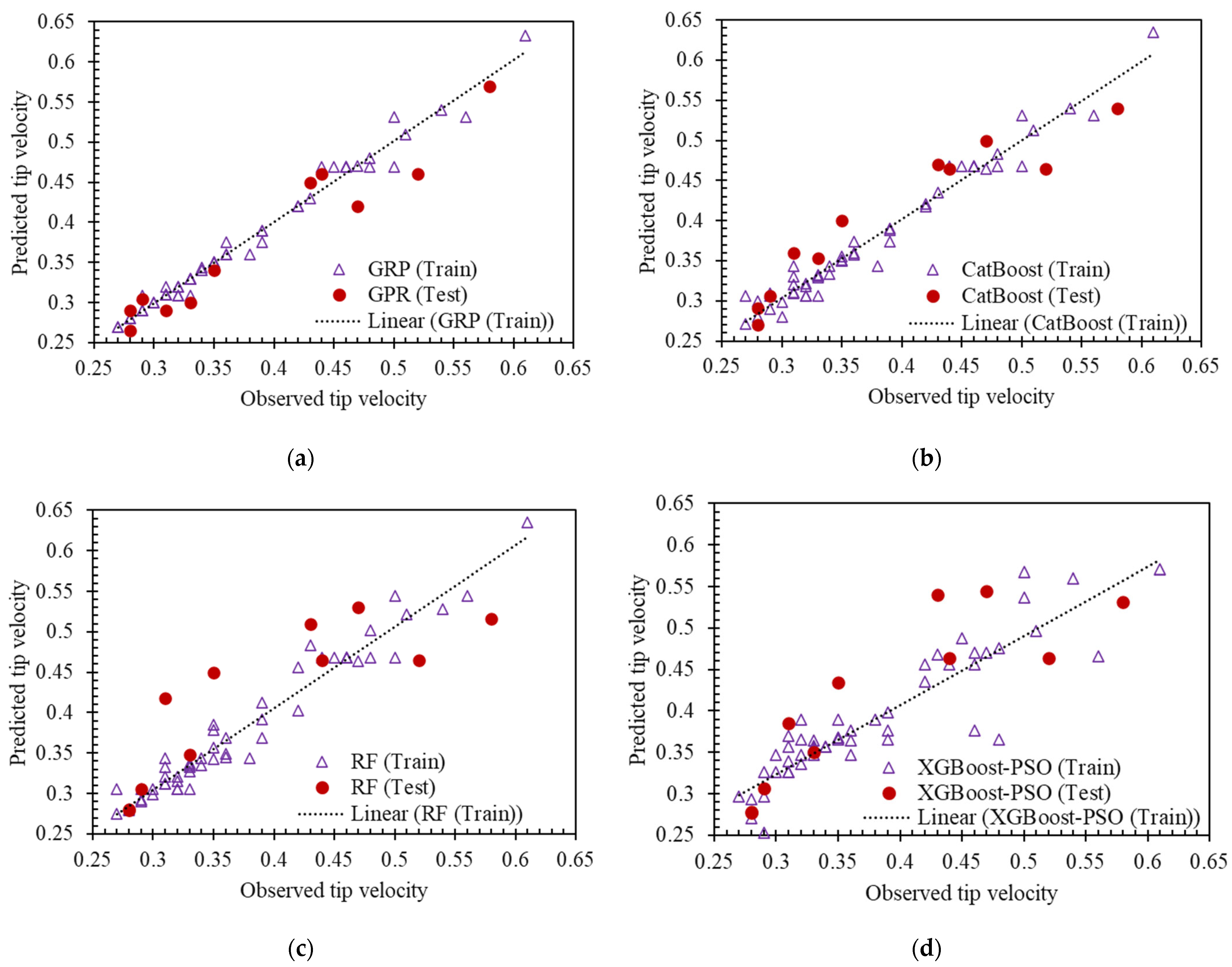
The significant predictive power indicated by GPR models was due to their kernel-based function contribution in the case of small- or medium-sized data points with nonlinearity. The findings align with previous studies [46,47] that concluded that the GPR model can enhance the prediction of hydraulic phenomena because of GPR’s capability for handling uncertainty and adaptation to the fluctuations. Because of categorical features and avoiding the overfitting issue, the predictive performance of the CatBoost model aligns with the study conducted by [48], highlighting its good performance in the prediction of hydrodynamic phenomena with conventional gradient boosting. Thus, the findings of the present paper suggest the utilization of GPR and CatBoost models in the effective prediction of open channel hydraulics, including interactions between geometric and hydraulic circumstances. Although the RF model showed somewhat moderate performance compared to the other two models, in general, its performance was accurate in predicting tip velocity in the vicinity of the spur dike. This aligns with the work of Breiman [37], which highlighted RF’s robustness and noise tolerance, explaining its stable but slightly lower predictive performance compared to boosting and probabilistic models. The poor performance of the RF model compared to the other three models demonstrates that the XGBoost–PSO model gave a weaker performance because of a smaller data series. Previous studies have reported that the XGBoost–PSO model performed well in predicting hydrodynamic phenomena with larger data series and fine-tuned hyperparameters [48,49,50]. The predicted values of the tip velocity using four different AI models are depicted in Figure 8a–d. The findings of this paper recommend the utilization of advanced AI models, including GPR and CatBoost, in the prediction of flow characteristics around a spur dike in an open channel under diverse hydraulic and geometrical configurations.

3.5. Residual Analysis

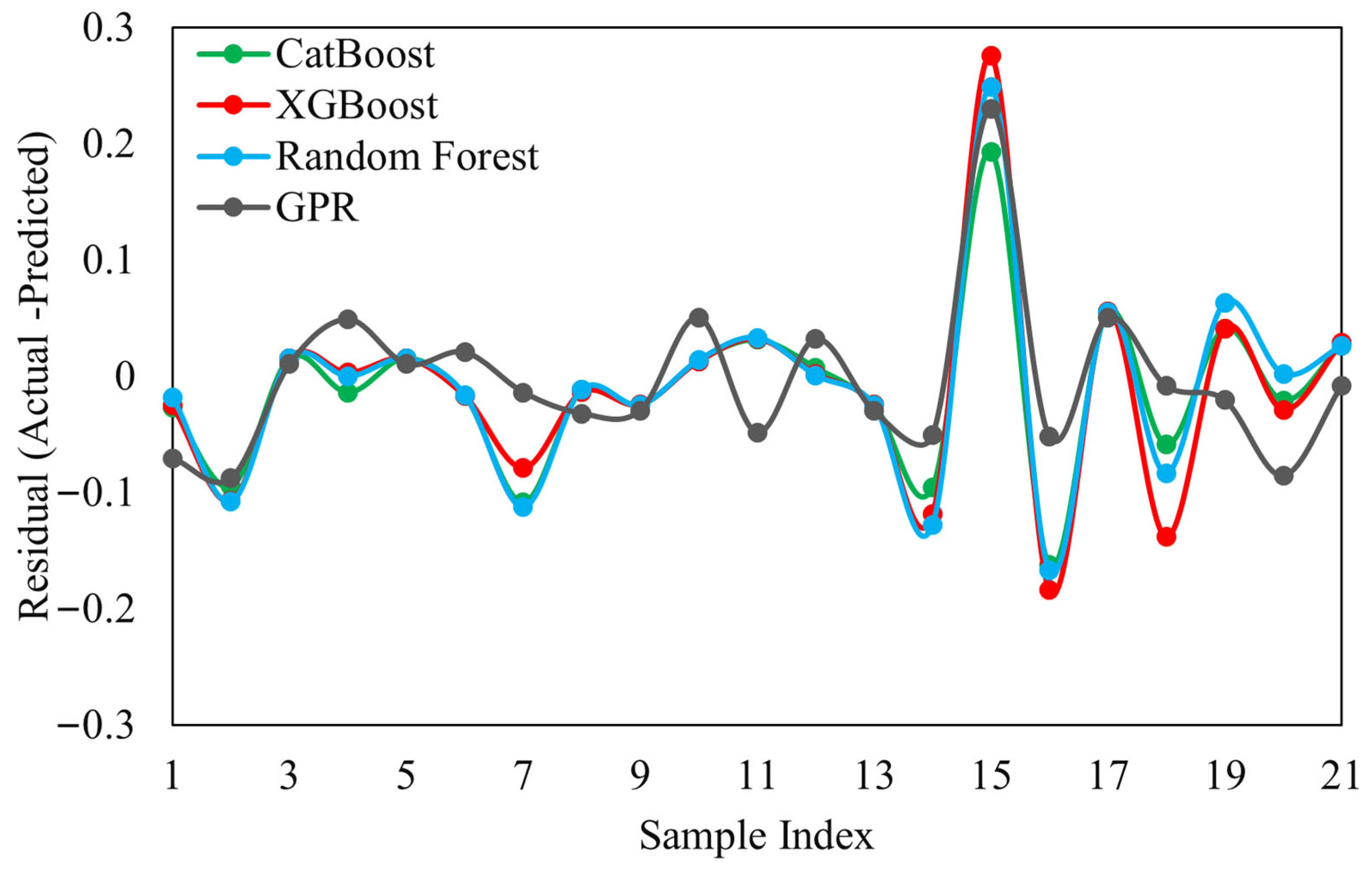
In this study, residual analysis was performed to evaluate the statistical performance by evaluating the error between actual and residual values to point out issues like poor model fit performance, assumptions, nonlinearity, and outliers. The residual analysis of the four tuned CatBoost, XGBoost–PSO, Random Forest, and Gaussian Process Regression (GPR) models gives further insight into the accuracy of predictions and the distribution of error used in estimating the tip velocity around spur dikes (Figure 9). In the best scenario, the residual additionally has to show a non-uniform and importantly random distribution around zero, indicating objective and precise predictions. GPR had the least varied residual pattern in this study, with the most residuals and relatively smooth variability about the zero line across the test samples. This indicates that the nonlinear relationships among the hydraulic parameters were observed with GPR, hence reducing the tendencies of under- and overprediction. CatBoost also showed a high performance, and the values of the residuals were concentrated close to zero values, but when some small deviations in treatment at certain sample identities occurred, they revealed a small sensitivity of CatBoost to the local differentiation of flow conditions.

The Random Forest residuals displayed a moderate distribution of data in contrast to GPR and CatBoost. Although the model predicted evenly, it occasionally oscillated up and down around zero, indicating some overfitting to the local patterns in the training data. However, its residual magnitudes remained acceptable, which attests to the strength of RF as a nonparametric ensemble-based method. Conversely, the biggest residual range of XGBoost–PSO corresponded to greater deviations, which were between sample values of 14 and 16. These spikes resolved to systematic prediction errors, in which the model failed to effectively generalize across some cases of the test but still tuned its parameters. This is consistent with the previously mentioned performance measures, as XGBoost–PSO had a relatively larger error as well as poorer overall predictive accuracy. A more detailed look at the residual trends also reveals that no model exhibited heteroscedasticity because the dispersion of values was relatively stable among test indexes. This supports the predictive stability of the models over the dataset. Nonetheless, all models have outliers, which may suggest that further modeling would benefit from hybridization or further feature engineering to minimize localized variations. The residual analysis proves that GPR gave the most available and stable predictions, closely followed by CatBoost. Random Forest also performed reasonably well with slightly more variability, whereas XGBoost–PSO was not entirely reliable because more frequent occurrences of zero-derived deviations were observed.

3.6. Quantile Analysis

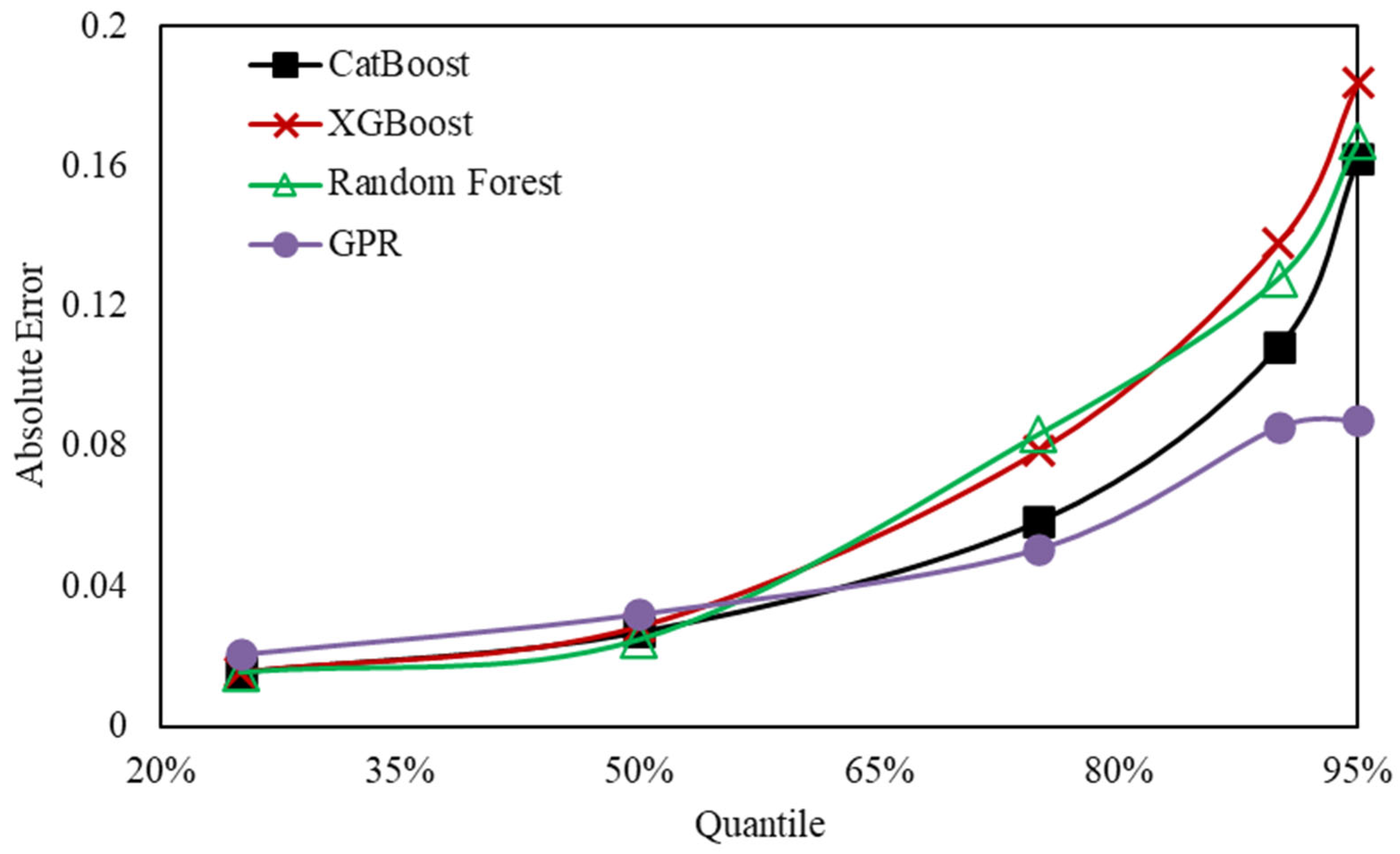
In this study, quantile analysis was performed, which employed statistical techniques for understanding the relationship between input and output parameters across various quantiles rather than relying on the mean value. This analysis gives absolute errors across various levels for a deeper understanding of model performance, robustness, and distribution. Figure 10 depicts the quantile analysis performed in this study. The quantile analysis was performed for four AI models, including GPR, CatBoost, RF, and XGBoost–PSO. Each of the tested models showed different levels of prediction precision across different quantiles. Under lower quantile values of 25% and 50%, the plot of quantile analysis showed smaller values of absolute error, as can be seen from the plot. GPR and CatBoost models showed somewhat more stability compared to RF and XGBoost–PSO models. The result presented in the quantiles analysis depicts most of the predicted values around the median; hence, all models showed precision and accuracy of the targeted parameter with lower deviation from the observed tip velocity in the vicinity of the spur dike. This is, however, different when the quantile goes to 75%, 90%, and 95%. XGBoost reported the highest absolute error change, especially for the 90% and 95% quantile points, where the error exceeded 0.18. The implication is that XGBoost might not have a high level of stability in extreme datasets or tail networks in terms of average performance. Random Forest demonstrated a lower, although steadier growth in error, which topped out at about 0.165 at the 95% quantile, indicating its susceptibility to somewhat overfitting noise in complex data. CatBoost, however, bounded relatively smaller errors to 90 percent and did not increase sharply until the 95 percent mark, indicating superior flexibility and generalization over most of the data, which are also prone to extreme values. GPR showed the most consistent performance at the quantile, and overall, the error growth was comparatively lower at the 95% quantile, which showed that it best represents the underlying functional relationship. Such trends may be attributed to the properties of every algorithm. XGBoost is a highly sensitive algorithm, which in the worst case can exaggerate errors. Random Forest predicts by averaging decision trees and producing lower variance while still collecting errors at the extremes. The gradient boosting model utilized by CatBoost to regulate categorical variables and ordered boosting makes it more stable. Meanwhile, GPR makes use of kernel-based learning, which offers less pointed predictions and is more unsusceptible to noise, as noted by relatively smaller quantile errors. The quantile result supports the idea that although any of the models can be relied on to make average predictions, GPR and CatBoost are more robust, especially when the error is considered to be higher.

3.7. SHAP Analysis

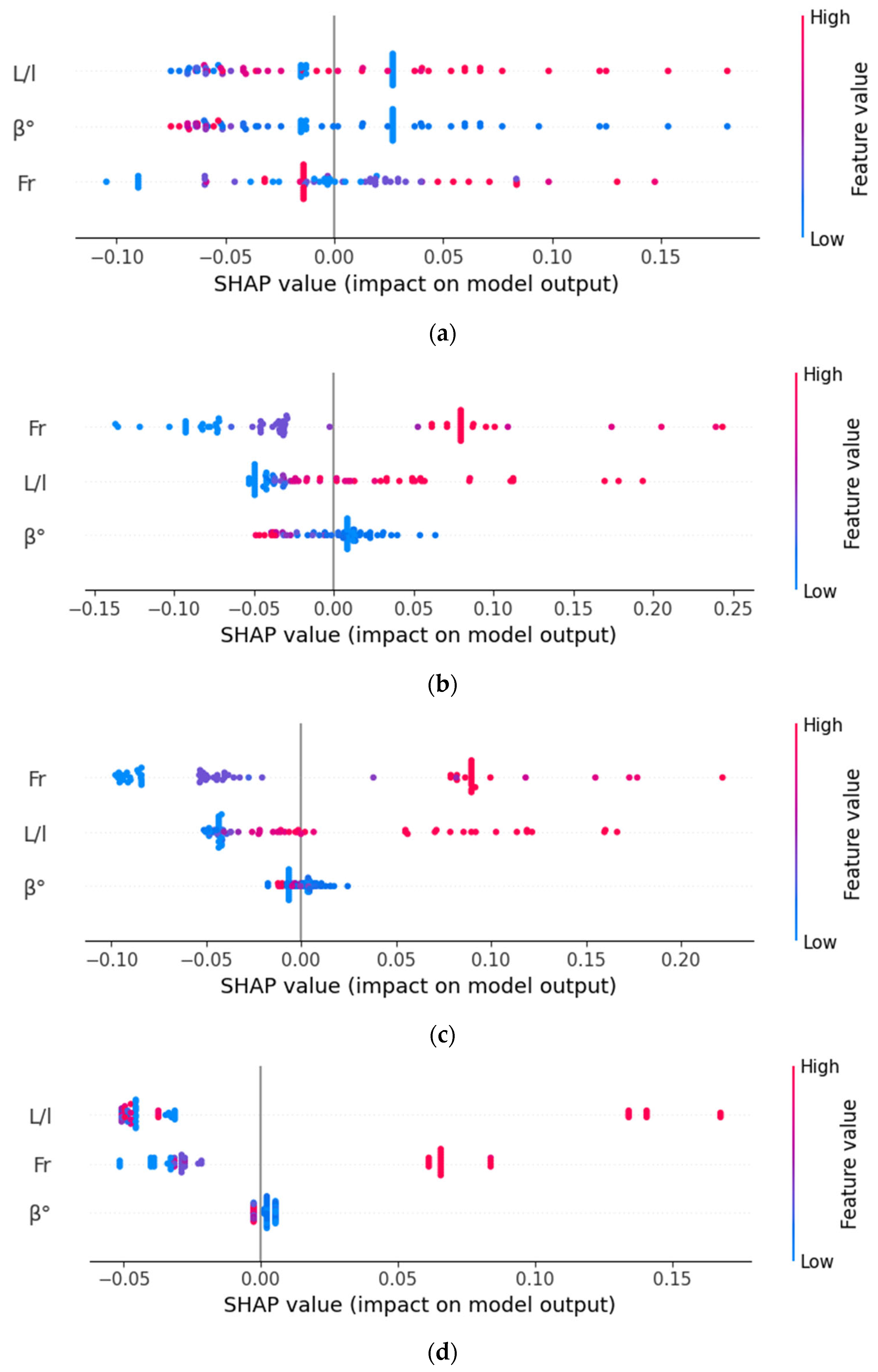
In this section, a detailed assessment of SHAP analysis is presented, which shows the relative impact of various input parameters on the targeted parameter across four different AI models. In this study, a tip velocity in the vicinity of the spur dike was predicted using input parameters like L/l, Fr, and β, as shown in Figure 11. The four AI models utilized in this study were GPR, CatBoost, RF, and XGBoost–PSO. The result presented in Figure 11a indicates that parameters related to flow regimes, especially Fr, show a higher positive impact on the prediction of tip velocity in the vicinity of the spur dike. Figure 11a depicts the result of SHAP analysis in the case of the GPR model, which demonstrated that L/l contributed significantly, with the SHAP value ranging between −0.08 to 0.20. Following L/l, the incidence angle (β) showed almost a similar contribution to the prediction of the tip velocity in the case of the GPR model. However, in the case of Fr, the SHAP value of the predicted tip velocity ranged between −0.11 and 0.15. Further, in the case of the CatBoost model, as shown in Figure 11b, the result demonstrated SHAP values between −0.15 and 0.25, −0.05 and 0.20, and −0.05 and 0.07 for Fr, L/l, and β, respectively. The result presented in Figure 11b demonstrated that in the case of the CatBoost model, flow regimes like Fr had a greater impact on the prediction of tip velocity compared to L/l and β. Following GPR and CatBoost, in this study, the impact of input parameters on the predicted values of tip velocity in the case of RF was evaluated. The results show that in the case of the RF model, Fr had greater influence on the predicted value of tip velocity, with SHAP values ranging between −0.10 and 0.23 (Figure 11c). Meanwhile, the L/l showed a moderate impact on the predicted value of tip velocity in the case of the RF model, with SHAP values ranging between −0.05 to 0.17. The least influence of β was observed on the predicted value of the tip velocity in the case of the RF model, with SHAP value ranging from −0.02 to 0.03. Following the result of the CatBoost model, the RF model also demonstrated that Fr has a greater impact on the predicted values of the tip velocity. Furthermore, in the case of the XGBoost–PSO model, it was noticed that the input parameter (L/l) had a greater impact on the predicted values of tip velocity compared to Fr and β. The order of the input parameters influencing tip velocity in the vicinity of the spur dike is L/l > Fr > β (Figure 11d).

The result of the SHAP analysis confirmed a physical phenomenon where greater flow velocity, represented by Fr, greatly influenced local velocities and turbulence structures, while geometrical consideration of the spur dike and flow separation altered vortex shedding and flow contraction phenomenon along the tip of the dike. In contrast, the incidence angle showed moderate contribution to the flow alteration, acting as a secondary option in the field of river engineering, as in the real-world scenario in which a spur dike is usually installed at a right angle to the flow direction. Furthermore, the result of the SHAP analysis validated the real-world scenarios where flow regimes are greatly influenced by the geometrical configuration of the spur dike. The interpretability of SHAP also further closed the gap between the AI-based modeling and understanding of the hydraulic phenomenon, confirming actual correspondence between the physical principles of spur dike-induced flow change and data-driven knowledge. Therefore, these results provide greater confidence in implementing optimized artificial intelligence models for the prediction of tip velocity in hydraulic engineering and underline that achieving prediction and interpretability can be combined for designing optimized solutions and risk assessment for a spur dike in the field of river engineering.

4. Conclusions

In this paper, a detailed evaluation of different artificial intelligence (AI) methods was performed utilizing laboratory-scale data series collected from the literature to predict tip velocity around the spur dike of different hydraulic and geometrical conditions. In this paper, a total of 69 data points were collected from the literature with the input parameters of Froude number (Fr), separation length ratio (L/l), and incidence angle (β), and tip velocity was considered as a targeted parameter. Based on the collected data points, four various AI models were utilized, including Gaussian Process Regression (GPR), Categorical Boosting (CatBoost), Random Forest (RF), and Extreme Gradient Boosting (XGBoost) with Particle Swarm Optimization (PSO), by assigning 70%, 15%, and 15% data point to the training, testing, and validation phases. Once each model was trained and optimized, the performance was evaluated through the Coefficient of Determination (R2) and Root Mean Square Error (RMSE). Furthermore, model robustness was assessed through residual and quantile analysis, while SHAP analysis was performed to understand the influence of input parameters on the tip velocity in the vicinity of the spur dike. The conclusion of this research is the following:

• The result of the correlation heatmap concluded that Fr demonstrated greater correlation with tip velocity, with a correlation coefficient (R) value of 0.71. This shows that under greater values of Fr, the flow significantly altered the flow acceleration near the tip of the dike, improving the risk of erosion and turbulence. In contrast, incidence angle (β) demonstrated a negative correlation with the R value of −0.37;
• The result of the AI model’s performance demonstrated superior performance of the GPR model compared to others, with an R2 value of 0.972 and an RMSE value of 0.0107. This demonstrated that the GPR model has superior performance because of its flexibility based on the kernel function and its small dataset handling capability. In contrast, the XGBoost–PSO model has a lower value of R² = 0.810 and RMSE = 0.0586, demonstrating weaker performance;
• Residual analysis showed that GPR and CatBoost yielded the most consistent predictions, with the residuals being concentrated on zero, which indicated a low under- or overprediction rate. RF was capable of moderately varying, though it was reliable, whereas XGBoost–PSO had made the highest residual deviations. Quantile-based analysis validated the fact that GPR and CatBoost had a steady performance in accuracy evaluation throughout the distribution of data, whereas RF had a steady but marginally greater errors at heavy quantiles, and XGBoost–PSO had instability when dealing with small data.

The result concluded from this study is only valid for a single-spur-dike system, and future studies should integrate parameters from a series of spur dike systems and their spacing to capture the applicability of the result at a large scale and for complex river-training structures. The dataset has only four input parameters, but these parameters are the key hydraulic variables controlling tip velocity within the experimental settings of Yeo et al. [34]. AI models not only work efficiently in high-dimensional data but also in nonlinear interactions in low-dimensional systems. The interactions between Fr, β, and L/l in the current study were nonlinear enough that AI models had superior predictive power compared to conventional methodologies. The relevance of the methodology to field conditions of more complexity remains to be tested with future datasets that consider other parameters like sediment particles, turbulence measures, and the spacing of dikes and the geometrical changes of a channel. The addition of more parameters in future research will further challenge the suitability and applicability of AI techniques to spur-dike hydraulic analysis.

Future studies should focus on larger data series based on laboratory settings or field observation to enhance the generalization of AI models. Physics-informed models and hybrid physics-informed models (AI) could be improved in terms of interpretability and robustness under a variety of flow conditions. Furthermore, future research should investigate the prediction of tip velocity under diverse sediment particle diameters, unsteady flow conditions, and a group of spur dikes. The application of these models to climate-induced hydrological changes and real-time observation of rivers would be important steps forward concerning the sustainable design and stability of spur dike systems in river engineering.

References

1. Nandhini, D.; Murali, K.; Harish, S.; Schüttrumpf, H.; Heins, K.; Gries, T. A state-of-the-art review of normal and extreme flow interaction with spur dikes and its failure mechanism. Phys. Fluids 2024, 36, 051301. [Google Scholar] [CrossRef] [Scilit]
2. Mostafa, M.M.; Ahmed, H.S.; Ahmed, A.A.; Abdel-Raheem, G.A.; Ali, N.A. Experimental study of flow characteristics around floodplain single groyne. J. Hydro-Environ. Res. 2019, 22, 1–13. [Google Scholar] [CrossRef] [Scilit]
3. Patel, H.K.; Arora, S.; Lade, A.D.; Kumar, B.; Azamathulla, H.M. Flow behaviour concerning bank stability in the presence of spur dike—A review. Water Supply 2023, 23, 237–258. [Google Scholar] [CrossRef] [Scilit]
4. Liu, D.; Lv, S.; Li, C. Impact of Spur Dike Placement on Flow Dynamics in Curved River Channels: A CFD Study on Pick Angle and River-Width-Narrowing Rate. Water 2024, 16, 2236. [Google Scholar] [CrossRef] [Scilit]
5. Chakravarty, S.; Patel, H.K.; Mohanty, B.; Kumar, B. Review on different shapes of spurs and their effects on channel morphology. Water Pract. Technol. 2024, 19, 241–262. [Google Scholar] [CrossRef] [Scilit]
6. Iqbal, S.; Siddique, M.; Hamza, A.; Murtaza, N.; Pasha, G.A. Computational analysis of fluid dynamics in open channel with the vegetated spur dike. Innov. Infrastruct. Solut. 2024, 9, 345. [Google Scholar] [CrossRef] [Scilit]
7. Giglou, A.N.; Mccorquodale, J.A.; Solari, L. Numerical study on the effect of the spur dikes on sedimentation pattern. Ain Shams Eng. J. 2018, 9, 2057–2066. [Google Scholar] [CrossRef] [Scilit]
8. Pandey, M.; Lam, W.H.; Cui, Y.; Khan, M.A.; Singh, U.K.; Ahmad, Z. Scour around Spur Dike in Sand–Gravel Mixture Bed. Water 2019, 11, 1417. [Google Scholar] [CrossRef] [Scilit]
9. Hussein, I.H.; Jamel, A.A.J.; Irzooki, R.H. Environmental and Hydraulic Considerations in Scour Reduction Around Spur Dikes: A Comprehensive Review. Sustain. Mar. Struct. 2025, 7, 117–135. [Google Scholar] [CrossRef] [Scilit]
10. Iqbal, S.; Haider, R.; Pasha, G.A.; Zhao, L.; Abbas, F.M.; Anjum, N.; Murtaza, N.; Abbas, Z. Numerical Investigation of Flow Around Partially and Fully Vegetated Submerged Spur Dike. Water 2025, 17, 435. [Google Scholar] [CrossRef] [Scilit]
11. Pradhan, T.K.; Malasani, G.C.; Reddy, S.K.; Chandra, V. Investigation on scouring and turbulence characteristics around T-head spur dike. J. Appl. Water Eng. Res. 2024, 12, 323–338. [Google Scholar] [CrossRef] [Scilit]
12. Akbar, Z.; Murtaza, N.; Pasha, G.A.; Iqbal, S.; Ghumman, A.R.; Abbas, F.M. Predicting scour depth in a meandering channel with spur dike: A comparative analysis of machine learning techniques. Phys. Fluids 2025, 37, 045158. [Google Scholar] [CrossRef] [Scilit]
13. Koken, M.; Gogus, M. Effect of spur dike length on the horseshoe vortex system and the bed shear stress distribution. J. Hydraul. Res. 2015, 53, 196–206. [Google Scholar] [CrossRef] [Scilit]
14. Koken, M.; Constantinescu, G. Flow and turbulence structure around a spur dike in a channel with a large scour hole. Water Resour. Res. 2011, 47, W12511. [Google Scholar] [CrossRef] [Scilit]
15. Akbar, Z.; Pasha, G.A.; Tanaka, N.; Ghani, U.; Hamidifar, H. Reducing bed scour in meandering channel bends using spur dikes. Int. J. Sediment Res. 2024, 39, 243–256. [Google Scholar] [CrossRef] [Scilit]
16. Gu, Z.; Cao, X.; Gu, Q.; Lu, W.-Z. Exploring Proper Spacing Threshold of Non-Submerged Spur Dikes with Ipsilateral Layout. Water 2020, 12, 172. [Google Scholar] [CrossRef] [Scilit]
17. Iqbal, S.; Pasha, G.A.; Ghani, U.; Ullah, M.K.; Ahmed, A. Flow Dynamics Around Permeable Spur Dike in a Rectangular Channel. Arab. J. Sci. Eng. 2021, 46, 4999–5011. [Google Scholar] [CrossRef] [Scilit]
18. Özyaman, C.; Yerdelen, C.; Eris, E.; Daneshfaraz, R. Experimental investigation of scouring around a single spur under clear water conditions. Water Supply 2022, 22, 3484–3497. [Google Scholar] [CrossRef] [Scilit]
19. Aydogdu, M. CFD technology in innovative spur dike design inspired by the Eğri (curved) Bridge. Sci. Rep. 2025, 15, 21308. [Google Scholar] [CrossRef] [Scilit] [PubMed]
20. Vaghefi, M.; Mahmoodi, K.; Setayeshi, S.; Akbari, M. Application of artificial neural networks to predict flow velocity in a 180° sharp bend with and without a spur dike. Soft Comput. 2020, 24, 8805–8821. [Google Scholar] [CrossRef] [Scilit]
21. Singh, B.; Minocha, V.K. Comparative Study of Machine Learning Techniques for Prediction of Scour Depth around Spur Dikes. In Proceedings of the World Environmental and Water Resources Congress 2024, Milwaukee, WI, USA, 19–22 May 2024; American Society of Civil Engineers: Reston, VA, USA, 2024; pp. 635–651. [Google Scholar] [CrossRef] [Scilit]
22. Wei, X.; Lu, Y.; Wang, Z.; Liu, X.; Mo, S. A Machine Learning Approach to Evaluating the Damage Level of Tooth-Shape Spur Dikes. Water 2018, 10, 1680. [Google Scholar] [CrossRef] [Scilit]
23. Tabassum, R.; Guguloth, S.; Gondu, V.R.; Zakwan, M. Machine learning-based prediction of scour depth evolution around spur dikes. J. Hydroinform. 2024, 26, 2815–2836. [Google Scholar] [CrossRef] [Scilit]
24. Pandey, M.; Jamei, M.; Ahmadianfar, I.; Karbasi, M.; Lodhi, A.; Chu, X. Assessment of scouring around spur dike in cohesive sediment mixtures: A comparative study on three rigorous machine learning models. J. Hydrol. 2022, 606, 127330. [Google Scholar] [CrossRef] [Scilit]
25. Saber, A.I.M.; Hassan, H.T.A. The Impact of Spur Dikes on the Dynamics of Erosion and Deposition Processes in the Nile River in Abnub Area: A Study in Engineering Geomorphology Using Artificial Intelligence. J. Fac. Arts Port Said Univ. 2024, 27, 172–223. [Google Scholar] [CrossRef] [Scilit]
26. Singh, B.; Minocha, V.K. An optimized boosting-based machine learning model for predicting maximum scour depth around spur dikes. Mar. Georesour. Geotechnol. 2025, 1–21. [Google Scholar] [CrossRef] [Scilit]
27. Singh, B.; Minocha, V.K. Approximation in scour depth around spur dikes using novel hybrid ensemble data-driven model. Water Sci. Technol. 2024, 89, 962–975. [Google Scholar] [CrossRef] [Scilit] [PubMed]
28. Gupta, L.K.; Pandey, M.; Raj, P.A. Numerical modeling of scour and erosion processes around spur dike. CLEAN—Soil Air Water 2025, 53, 2300135. [Google Scholar] [CrossRef] [Scilit]
29. Yeo, H.K.; Kang, J.G.; Kim, S.J. An experimental study on tip velocity and downstream recirculation zone of single groynes of permeability change. KSCE J. Civ. Eng. 2005, 9, 29–38. [Google Scholar] [CrossRef] [Scilit]
30. Malekjani, N.; Kharaghani, A.; Tsotsas, E. A comparative study of dimensional and non-dimensional inputs in physics-informed and data-driven neural networks for single-droplet evaporation. Chem. Eng. Sci. 2025, 306, 121214. [Google Scholar] [CrossRef] [Scilit]
31. Zhang, J.; Zhang, S.; Zhang, J.; Wang, Z. Machine Learning Model of Dimensionless Numbers to Predict Flow Patterns and Droplet Characteristics for Two-Phase Digital Flows. Appl. Sci. 2021, 11, 4251. [Google Scholar] [CrossRef] [Scilit]
32. Rezzoug, A.; Khan, A.; Murtaza, N.; Rizvi, S.A.S. Predicting flood energy reduction in vegetated open channel: Comparative assessment of hybrid artificial intelligence techniques. Eng. Appl. Artif. Intell. 2025, 159, 111756. [Google Scholar] [CrossRef] [Scilit]
33. Murtaza, N.; Khan, D.; Rezzoug, A.; Khan, Z.U.; Benzougagh, B.; Khedher, K.M. Scour depth prediction around bridge abutments: A comprehensive review of artificial intelligence and hybrid models. Phys. Fluids 2025, 37, 021306. [Google Scholar] [CrossRef] [Scilit]
34. Eini, N.; Bateni, S.M.; Jun, C.; Heggy, E.; Band, S.S. Estimation and interpretation of equilibrium scour depth around circular bridge piers by using optimized XGBoost and SHAP. Eng. Appl. Comput. Fluid Mech. 2023, 17, 2244558. [Google Scholar] [CrossRef] [Scilit]
35. Liu, C.; Duan, Z.; Zhang, B.; Zhao, Y.; Yuan, Z.; Zhang, Y.; Wu, Y.; Jiang, Y.; Tai, H. Local Gaussian process regression with small sample data for temperature and humidity compensation of polyaniline-cerium dioxide NH3 sensor. Sens. Actuators B Chem. 2023, 378, 133113. [Google Scholar] [CrossRef] [Scilit]
36. Han, S.; Williamson, B.D.; Fong, Y. Improving random forest predictions in small datasets from two-phase sampling designs. BMC Med. Inform. Decis. Mak. 2021, 21, 322. [Google Scholar] [CrossRef] [Scilit]
37. Breiman, L. Random forests. Mach. Learn. 2001, 45, 5–32. [Google Scholar] [CrossRef] [Scilit]
38. Jafari, R.; Sui, J. Velocity Field and Turbulence Structure around Spur Dikes with Different Angles of Orientation under Ice Covered Flow Conditions. Water 2021, 13, 1844. [Google Scholar] [CrossRef] [Scilit]
39. Duan, J.G.; He, L.; Fu, X.; Wang, Q. Mean flow and turbulence around experimental spur dike. Adv. Water Resour. 2009, 32, 1717–1725. [Google Scholar] [CrossRef] [Scilit]
40. Vaghefi, M.; Shakerdargah, M.; Akbari, M. Numerical investigation of the effect of Froude number on flow pattern around a submerged T-shaped spur dike in a 90° bend. Turk. J. Eng. Environ. Sci. 2014, 38, 266–277. [Google Scholar] [CrossRef] [Scilit]
41. Jeon, J.; Lee, J.Y.; Kang, S. Experimental Investigation of Three-Dimensional Flow Structure and Turbulent Flow Mechanisms Around a Nonsubmerged Spur Dike with a Low Length-to-Depth Ratio. Water Resour. Res. 2018, 54, 3530–3556. [Google Scholar] [CrossRef] [Scilit]
42. Li, Y.-T.; Zhan, J.-M.; Wai, W.-H.O. A study of the effect of local scour on the flow field near the spur dike. Theor. Appl. Mech. Lett. 2024, 14, 100510. [Google Scholar] [CrossRef] [Scilit]
43. Kang, J.G.; Yeo, H.-K.; Kim, S.-J. An Experimental Study on Tip Velocity and Downstream Recirculation Zone of Single Groyne Conditions. J. Korea Water Resour. Assoc. 2005, 38, 143–153. [Google Scholar] [CrossRef] [Scilit]
44. Ho, J.; Yeo, H.K.; Coonrod, J.; Ahn, W.-S. Numerical Modeling Study for Flow Pattern Changes Induced by Single Groyne. In Proceedings of the Congress-International Association for Hydraulic Research 2007, Venice, Italy, 1–6 July 2007. [Google Scholar]
45. Li, G.; Sui, J.; Sediqi, S. Turbulent flow structure around a single submerged angled spur dike under ice cover. J. Hydrol. Hydromech. 2024, 72, 522–537. [Google Scholar] [CrossRef] [Scilit]
46. Rastgou, M.; Bayat, H.; Mansoorizadeh, M.; Gregory, A.S. Prediction of soil hydraulic properties by Gaussian process regression algorithm in arid and semiarid zones in Iran. Soil Tillage Res. 2021, 210, 104980. [Google Scholar] [CrossRef] [Scilit]
47. Park, J.; Lechevalier, D.; Ak, R.; Ferguson, M.; Law, K.H.; Lee, Y.-T.T.; Rachuri, S. Gaussian Process Regression (GPR) Representation in Predictive Model Markup Language (PMML). Smart Sustain. Manuf. Syst. 2017, 1, 121–142. [Google Scholar] [CrossRef] [Scilit]
48. Cai, Y.; Yuan, Y.; Zhou, A. Predictive slope stability early warning model based on CatBoost. Sci. Rep. 2024, 14, 25727. [Google Scholar] [CrossRef] [Scilit]
49. Zivkovic, M.; Jovanovic, L.; Ivanovic, M.; Bacanin, N.; Strumberger, I.; Joseph, P.M. XGBoost Hyperparameters Tuning by Fitness-Dependent Optimizer for Network Intrusion Detection. In Communication and Intelligent Systems; Springer: Singapore, 2022; pp. 947–962. [Google Scholar] [CrossRef] [Scilit]
50. Xiong, J.; Gong, Y.; Liu, X.; Li, Y.; Chen, L.; Liao, C.; Zhang, C. A PSO-XGBoost Model for Predicting the Compressive Strength of Cement–Soil Mixing Pile Considering Field Environment Simulation. Buildings 2025, 15, 2740. [Google Scholar] [CrossRef] [Scilit]
Figure 1. Schematic of flow around a spur dike showing separation, vortices, and recirculation zones that control turbulence.
Water 18 00026 g001
Figure 2. Flowchart of the methodology of models for predicting hydraulic behavior near spur dikes.
Water 18 00026 g002
Figure 3. Correlation heatmap representing how Fr, L/l, and β influence tip velocity and key flow interactions around the spur dike.
Water 18 00026 g003
Figure 4. Scatter pair plots illustrating nonlinear relationships among hydraulic/geometric variables and their effect on tip velocity.
Water 18 00026 g004
Figure 5. Regression plots showing how each input parameter (Fr, L/l, and β) affects tip velocity near the spur dike.
Water 18 00026 g005
Figure 6. Performance metrics were reported from the 5-fold cross-validation for four different tested models in this study. (a) R2 values across 5-fold cross-validation for the four tested models, (b) Root Mean Square Error (RMSE) values across 5-fold cross-validation for the four tested models.
Water 18 00026 g006
Figure 7. Performance metrics of various artificial intelligence models demonstrating the accuracy of AI models in capturing flow behavior near the spur dike.
Water 18 00026 g007
Figure 8. Relationship between observed and predicted values of the tip velocity under different hydraulic and geometrical configurations using four different models (a) GPR; (b) CatBoost; (c) RF; (d) XGBoost–PSO.
Water 18 00026 g008
Figure 9. Result of residual analysis for different AI models.
Water 18 00026 g009
Figure 10. Result of quantile analysis for different AI models.
Water 18 00026 g010
Figure 11. SHAP analysis showing the relative importance of Fr, L/l, and β in influencing tip velocity predictions (a) GPR; (b) CatBoost; (c) RF; (d) XGBoost–PSO.
Water 18 00026 g011