Study on the Influence Mechanism of Extreme Precipitation on Rice Yield in Hunan from 2000 to 2023 and the Countermeasures of Agricultural Production

Abstract

Hunan Province from 2000 to 2023 is the study area. Based on NOAA precipitation data and county-level rice yield statistics in Hunan Province, the Mann–Kendall test, extreme precipitation indices, and wavelet analysis examine the spatial and temporal evolution characteristics of extreme precipitation and its multi-scale impact on rice yield. The results show that the extreme precipitation in Hunan Province showed a stable pattern of fluctuation, and the main extreme precipitation indexes had no significant change trend. The spatial distribution showed a pattern of “high value in central-northern Hunan and stable in southern Hunan”, and the precipitation was concentrated in June–August. The rice yield showed the characteristics of “stable increase in the core area, intensified fluctuation in the transition area, and continuous shrinkage in the marginal area”, and the Dongting Lake Plain was a high-yield and stable area. Multi-scale analysis shows significant coupling between extreme precipitation and yield: in the 4–8-year cycle, the peak value of precipitation lags behind the response of 1–2 years, and changes synchronously in a short period. The response of rice to extreme precipitation showed a threshold-type nonlinear characteristic. Moderate wetting was beneficial to stable yield, while the yield decreased significantly when the intensity or continuous precipitation exceeded the threshold. Hunan’s rice system has strong climate resilience but requires a multi-scale climate-adaptive agricultural system via engineering, technology, and policy for long-term stability and sustainable grain production.

1. Introduction

In the context of global climate change, the frequency and intensity of extreme climatic events have become major challenges to the sustainable development of agriculture worldwide [1,2,3]. According to the Sixth Assessment Report of the Intergovernmental Panel on Climate Change (IPCC), extreme precipitation has shown an increasing trend in most land regions, particularly in the East Asian monsoon zone [4,5,6]. Hunan Province, located in the transitional zone between the middle–lower Yangtze River Basin and South China, is characterized by complex terrain and strong monsoon precipitation. Interannual fluctuations in hydrometeorological conditions substantially influence agricultural production in this typical humid rice-growing area [7,8,9]. In recent years, short-duration heavy rainfall, concentrated rainstorms, and persistent Meiyu processes have intensified, posing potential risks to rice yield stability [10,11,12].

As one of the largest rice production regions in China, Hunan contributes nearly 10% of the national rice cultivation area, and its total output has ranked first nationwide for many years [13,14,15]. Because the rice growth period overlaps strongly with the rainy season, the rice yield is highly sensitive to precipitation variability [16,17,18]. Moderate wetting conditions promote tillering and grain filling, whereas excessive or prolonged precipitation may cause waterlogging, lodging, root hypoxia, and the proliferation of pests and diseases, ultimately leading to yield reduction risks [19,20,21]. Accurately identifying the variation characteristics of extreme precipitation and clarifying its multi-scale influence mechanism on rice yield therefore has important implications for evaluating the climate resilience of rice-cropping systems and formulating adaptive management strategies [22,23,24].

Although numerous studies have analyzed precipitation trends and crop responses at national or Yangtze River Basin scales, regional climatic regimes, topographic features, and agricultural infrastructure conditions result in considerable spatial heterogeneity in crop sensitivity to extreme precipitation [25,26,27]. The existing research on Hunan Province mainly focuses on the climatic background or crop simulation [28,29,30], but systematic and quantitative investigations on the multi-scale coupling relationship between extreme precipitation patterns and rice yield, particularly regarding threshold identification, lag effects, and spatial heterogeneity, remain insufficient [31,32,33].

To address these gaps, this study uses NOAA daily precipitation data and county-level rice yield statistics in Hunan Province during 2000–2023. The Mann–Kendall (MK) trend test, extreme precipitation indices, and wavelet analysis are applied to examine the following: the long-term temporal and spatial variation characteristics of extreme precipitation in Hunan Province; the magnitude, scale, and lag features of its impacts on rice yield; multi-scale adaptation strategies to enhance regional agricultural resilience and food security under increasing climate risks.

The main contributions of this study are threefold: A comprehensive depiction of extreme precipitation characteristics in Hunan Province is provided using multi-index, long-term observations [34,35]. A multi-scale lag-coupling mechanism between precipitation extremes and rice yield is revealed using wavelet analysis [36,37]. Based on statistical findings, a conceptual framework integrating “mechanism cognition–risk identification–adaptation strategy” is proposed to support climate-adaptive agricultural development in humid rice-growing regions [38,39].

2. Data and Methods

2.1. Overview of the Research Area

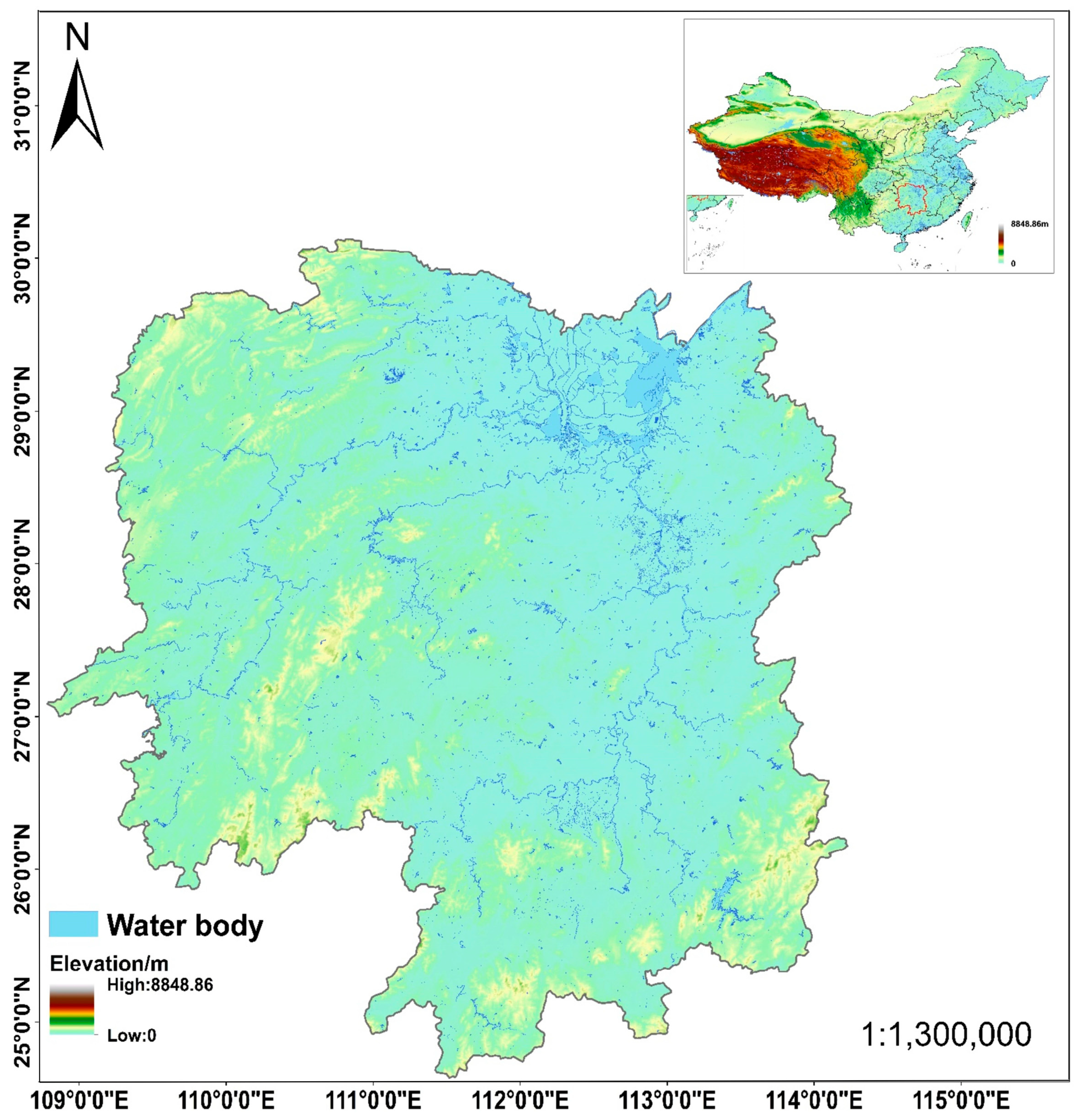
Hunan Province (24°38′–30°08′ N, 108°47′–114°15′ E) lies in the middle reaches of the Yangtze River, characterized by a subtropical monsoon humid climate. Annual precipitation averages between 1200 and 1700 mm, exhibiting uneven spatial and temporal distribution with concentrated summer rainfall and frequent extreme downpours. Its topography presents “mountains encircling three sides, opening northwards” configuration, with the Xiang, Zi, Yuan, and Li rivers converging into Dongting Lake, forming a complex water network. As a major rice-producing region nationally, it boasts over 4 million hectares of rice cultivation, accounting for 12–15% of China’s total output, with a high proportion of double-cropping rice. From 2000 to 2023, extreme precipitation intensity and frequency increased significantly, severely impacting rice yields through flood inundation, soil erosion, and exacerbated pest and disease outbreaks. This poses particular threats to production safety during the grain-filling to heading stages. This study aims to elucidate the underlying mechanisms and provide evidence for agricultural response strategies (Figure 1).

2.2. Data

To rigorously characterize spatiotemporal precipitation variability, we utilized daily observational records from the National Oceanic and Atmospheric Administration (NOAA) Global Historical Climatology Network (GHCN-Daily), covering the period from 2000 to 2023 (https://www.ncei.noaa.gov/data, accessed on 1 July 2025) [40]. While focusing on the 21st century, this archive is underpinned by a historical baseline spanning over 70 years, a temporal continuity that far surpasses the capabilities of most satellite-based products [41]. The robustness of the NOAA dataset stems from its stringent quality assurance protocols, including multi-site collaborative cross-checks and high-density spatial redundancy, which effectively mitigate single-source observational uncertainties [42]. Such standardized, high-fidelity records are indispensable for precise attribution analysis—specifically in quantifying the frequency, intensity, and spatiotemporal evolution of extreme weather anomalies [43,44]. Furthermore, this observational ground truth provides the critical physical boundary conditions necessary to validate numerical model simulations and assess climate-induced disaster risks with high confidence [45]. Daily precipitation data were obtained from the National Centers for Environmental Information (NCEI, NOAA). The original archive provides one comma-separated file (CSV) per station and year, where each record corresponds to the daily total precipitation (variable PRCP) for that station. The number of days with records per year is often less than 365 because many stations do not report continuously.

To construct a consistent dataset for analysis, we first merged all station–year CSV files and reorganized them into annual global files covering 1929–2024. For each year, we compiled the daily PRCP series for all available stations into a single table, so that each row corresponds to a station and each column to a calendar day. When a given station did not report on a particular day (i.e., there was no record in the original CSV), that station–day entry was treated as missing and stored as an empty cell in the tabular (Excel) version of the dataset.

The original PRCP values are reported in inches. All precipitation amounts were converted to millimeters using the standard factor 1 inch = 25.4 mm prior to any analysis.

The number of stations varies substantially over time, with many more stations operating in recent decades than in the early part of the record. For example, in 2024 the raw NCEI archive contains 12,159 stations with precipitation records. Stations with missing geographic coordinates (latitude and/or longitude) were retained in the attribute tables (Excel files), where their coordinates are stored as empty values, but were excluded from the spatial point datasets (shapefiles). As a result, the corresponding shapefile for 2024 contains 12,121 stations. All analyses that require spatial referencing (e.g., mapping, spatial statistics) are based only on stations with valid coordinates.

In the original NCEI CSV files, missing PRCP values are encoded as the numeric flag 99.99. During preprocessing, we handled missing values differently for tabular and spatial datasets. In the Excel files, 99.99 was replaced by an empty cell to explicitly represent missing data. In contrast, most GIS software automatically converts empty numeric fields to zero, which would make it impossible to distinguish “no precipitation” from “no observation”. Therefore, in the shapefiles we retained the value 99.99 as a sentinel code for missing precipitation and excluded these flagged values from all statistical and spatial analyses.

It is important to distinguish between zero precipitation and missing data. In our dataset, a PRCP value of 0 mm indicates that the station reported no precipitation for that day (and no precipitation was recorded in any sub-daily observation) according to the NCEI archive. However, we note that unreported precipitation events cannot be entirely ruled out. By contrast, missing values arise when a station has no daily record for a given calendar day in the original archive; such station–day combinations become empty (missing) entries when all stations are aligned on a common daily calendar. All analyses treat these missing entries as “no data” rather than zero rainfall.

Spatially explicit grain yield data were systematically compiled from the county-level Statistical Yearbooks of Hunan Province (2000–2023), constituting a comprehensive socio-economic panel dataset [46]. This inventory offers high administrative granularity and statistical integrity, capturing the complete production dynamics across county-level units with rigorous accuracy [47]. By integrating these agronomic records with meteorological variables, this study aims to disentangle the complex drivers governing yield variability [48]. Specifically, this coupled analysis provides an empirical basis for optimizing regional food security policies, ensuring resilience against shifting precipitation patterns and intensifying extreme events [49].

2.3. Method

2.3.1. Mann–Kendall and FDR

The UF and UB statistics in the Mann–Kendall (MK) trend test are key indicators for detecting mutation points in time series [50,51]. UF (forward sequence statistics) is used to identify the possible mutation points of the sequence from the starting point, while UB (reverse sequence statistics) verifies the reliability of the mutation points by reversing the sequence [52].

For time series X₁, X₂, ..., Xn of length n, the calculation steps for the UF statistic are as follows:

(1)

Calculate the sequence S_k:

$$S_k={\displaystyle \sum _{i=1}^k{s}_i}\hspace{1em}(k=2,3,\dots ,n)$$

(1)

where S_i is the comparative statistic, defined as

$$s_i={\displaystyle \sum _{j=1}^{i-1}\mathrm{sign}}\left(x_i-x_j\right),\hspace{1em}\mathrm{sign}(a)=\left\{\begin{array}{ll}1\hfill & \mathrm{if} a>0\hfill \\ 0\hfill & \mathrm{if} a=0\hfill \\ -1\hfill & \mathrm{if} a<0\hfill \end{array}\right.$$

(2)

(2)

Calculate the mean and variance of UF:

$$E\left[S_k\right]={\displaystyle \frac{k(k-1)}{4}}$$

(3)

$$\mathrm{Var}\left(S_k\right)={\displaystyle \frac{k(k-1)(2k+5)}{72}}$$

(4)

(3)

Standardization yields the UF statistic:

$${\mathrm{UF}}_k={\displaystyle \frac{S_k-E\left[S_k\right]}{\sqrt{\mathrm{Var}\left(S_k\right)}}}\hspace{1em}(k=2,3,\dots ,n)$$

(5)

UF1 is typically defined as 0.

Formula for calculating the UB statistic (reverse sequence):

UB is obtained by inverting the original sequence (i.e., y_i = x_{n + 1 − i}) and repeating the UF computation process, but ultimately requires adjustment of the sign and temporal order:

(1)

Reverse sequence: Let y = {x_n, x_{n − 1}, ..., x₁}.

(2)

Calculate the UF* statistic for the reversed sequence: Apply the UF formula to y to obtain UF_k^*.

(3)

Transform to obtain UB:

$${\mathrm{UB}}_k=-{\mathrm{UF}}_{n+1-k}^{*}\hspace{1em}(k=1,2,\dots ,n)$$

(6)

This conversion ensures that the UB is aligned with the original sequence’s timeline.

• Mutation point determination rules are as follows:

(1)

Significance test: Should |UF| or |UB| exceed the critical value, this indicates a significant trend change.

(2)

Inflection point identification: When the UF and UB curves intersect and the intersection point lies within the significance threshold range, the time corresponding to this intersection point constitutes the inflection point.

(3)

Trend direction: UF > 0 denotes an upward trend, while UF < 0 signifies a downward trend.

The role of UB is to validate the reliability of mutation points, thereby avoiding false positives.

Different from the traditional MK trend test, the UF–UB method is used to detect structural breaks rather than trend significance, so it does not provide a single Z value and p value, but judges the possibility of mutations through the change characteristics of UF and UB sequence curves.

FDR (false discovery rate) control is usually implemented by Benjamini–Hochberg (BH) program, which is a widely used statistical method for controlling the proportion of false discovery in multiple hypothesis testing [53,54,55].

(1)

Core Concept Definition

FDR (false discovery rate): Defined as the expected proportion of erroneous rejections (i.e., false discoveries) among all rejected null hypotheses (i.e., “discoveries”). Its mathematical expression is

$$\mathrm{FDR}=E\left[{\displaystyle \frac{V}{\max (R,1)}}\right]$$

(7)

where V denotes the number of false positives, and R denotes the total number of detections.

Benjamini–Hochberg (BH) procedure: Proposed by Yoav Benjamini and Yosef Hochberg in 1995, it is the most classical and widely applied method for controlling the false discovery rate (FDR). By adjusting the significance threshold, it balances discovery power and error control in multiple testing scenarios.

(2)

Operational steps for the BH program

Consider m independent hypothesis tests yielding m p-values. Given a target FDR level q, the BH procedure proceeds as follows:

• Sorting: Arrange the m p-values in ascending order, denoted as p₍₁₎ ≤ p₍₂₎ ≤ ... ≤ p_(m).
• Calculate the threshold: For each sorted p-value p(i), compute its corresponding BH threshold:

$${\displaystyle \frac{i}{m}}\cdot q$$

(8)

Comparison and determination: Find the largest index k such that

$$p_{(k)}\le {\displaystyle \frac{k}{m}}\cdot q$$

(9)

Then, reject all null hypotheses H₍₁₎, H₍₂₎, ..., H_(K).

Interpretation of results: All tests corresponding to P₍₁₎ through P_(k) were deemed statistically significant, and the FDR for this decision process was controlled below q.

2.3.2. Extreme Precipitation Index

This study aims to describe the seasonal characteristics of extreme precipitation in Hunan Province, China [56]. The extreme precipitation index system proposed by the International Panel on Climate Change Detection and Indices (IPCC) is widely used in this field. The system contains 11 core indicators (

Table 1. Classification of 11 extreme precipitation indices.

Classification	Index Code	Descriptive Metric	Mathematical Definition/Threshold	Unit
Duration and Quantity	CDD	Number of continuous drying days	The maximum continuous days of daily precipitation p < 1 mm	d
	CWD	Persistent wet days	The maximum continuous days of daily precipitation p ≥ 1 mm	d
	PRCPTOT	Total wet day precipitation	The cumulative sum of precipitation on wet days (p ≥ 1 mm)	mm
Frequency (Absolute)	R10	Number of moderate rain days	Days of daily precipitation p ≥ 10 mm	d
	R20	Days of heavy rain	Days of daily precipitation p ≥ 20 mm	d
	R50	Days of torrential rain	Days of daily precipitation p ≥ 50 mm	d
Extremes (Relative)	R95p	heavy rainfall	The cumulative sum of daily precipitation exceeding the 95th percentile	mm
	R99p	Extremely strong precipitation	The cumulative sum of daily precipitation exceeding the 99th percentile	mm
Intensity	Rx1day	Maximum daily precipitation	The maximum daily precipitation in the statistical period	mm
	RX5day	Maximum 5-day precipitation	The maximum value of the sum of any continuous 5-day precipitation	mm
	SDII	Simple precipitation intensity	Total wet day precipitation/wet day days	mm/d

) [57]. These indices cover the dimensions of precipitation intensity index, duration index and threshold index, which can fully reflect the intensity characteristics and frequency of seasonal extreme precipitation [58].

2.3.3. Single-Indicator Wavelet Cycle

To elucidate the inherent oscillatory modes embedded within the temporal datasets, we employed the Single-factor Wavelet Analysis method [59]. This technique facilitates a hierarchical decomposition of time series, effectively unmasking the latent periodic structures that govern both extreme precipitation anomalies and grain yield variability across diverse temporal scales [60]. Distinguished by its superior time–frequency localization capabilities, the wavelet transform serves as a rigorous diagnostic framework for detecting transient periodicities within non-stationary systems, overcoming the limitations of traditional spectral analysis [61]. The governing equation is defined as follows:

$$T=s\times t\times C$$

(10)

2.3.4. Wavelet Transform Coherence (WTC)

Wavelet transform coherence (WTC) provides a framework for assessing the time–frequency co-variability between two non-stationary time series. By characterizing correlations simultaneously in time and across spectral scales, WTC allows localized and scale-specific relationships to be identified, offering insights that conventional stationary analyses often miss [62,63]. The fundamental formulation is given as follows:

$$R_{xy}^2(s,\tau )={\displaystyle \frac{{\left|S\left[s^{-1}{W}_{xy}(s,\tau )\right]\right|}^2}{S\left[s^{-1}{\left|W_x(s,\tau )\right|}^2\right]\cdot S\left[s^{-1}{\left|W_y(s,\tau )\right|}^2\right]}}$$

(11)

2.3.5. Cross-Wavelet Transform (XWT)

Cross-wavelet transform (XWT) is a signal processing technology that analyzes the relationship between two time series in the time–frequency domain. By combining continuous wavelet transform and cross spectrum analysis, it can reveal the localization correlation characteristics and phase relationship of signals at multiple scales [64,65,66,67]. The core formula is as follows:

$$W_{xy}(s,\tau )=W_x(s,\tau )\cdot W_y^{\ast }(s,\tau )$$

(12)

2.3.6. Pearson Correlation Analysis

Pearson correlation analysis is a statistical method used to quantify the strength and direction of the linear relationship between two continuous variables [68,69]. It was proposed by British statistician Karl Pearson at the end of the 19th century [68,70]. The core of this method is to evaluate the correlation between variables by calculating the Pearson correlation coefficient [69,71]. Its core formula is as follows:

$$r={\displaystyle \frac{{\displaystyle \sum _{i=1}^n\left(X_i-\overline{X}\right)}\left(Y_i-\overline{Y}\right)}{\sqrt{{\displaystyle \sum _{i=1}^n{\left(X_i-\overline{X}\right)}^2}}\sqrt{{\displaystyle \sum _{i=1}^n{\left(Y_i-\overline{Y}\right)}^2}}}}$$

(13)

In the Pearson correlation analysis, this study used a two-tailed test, and the statistical significance level was set to α = 0.05.

When the t statistic corresponding to the calculated correlation coefficient r satisfies

$$\left|t\right|>t_{\alpha /2,df}$$

(14)

and when the corresponding p value is less than 0.05, it is considered that the linear relationship between extreme precipitation and rice yield is statistically significant.

The calculation formula of t value is

$$t=r\sqrt{{\displaystyle \frac{n-2}{1-r^2}}}$$

(15)

Degree of Freedom

According to the standard setting of Pearson correlation test, the degree of freedom (df) of this study is calculated as follows:

df = n − 2

where n is the number of sample pairs (years) involved in the relevant calculation.

The definition of this degree of freedom comes from the t distribution model of the correlation coefficient significance test, which is an international common treatment.

Data Alignment Method—Seasonal Synchronization

In order to ensure the comparability and consistency of the correlation between extreme precipitation and rice yield, this study used seasonal synchronization data alignment method.

The extreme precipitation index is calculated according to the four seasons of spring, summer, autumn, and winter (such as RX1day, RX5day, SDII, etc.). The rice yield data were paired according to the agricultural production season of the same year (represented by the annual yield of the county). The seasonal precipitation index of the same year is one-to-one corresponding to the rice yield of the year to ensure that the climatic variables and agricultural yield are analyzed at the same time scale.

3. Results

3.1. Spatial–Temporal Patterns of Extreme Precipitation Across Hunan Province

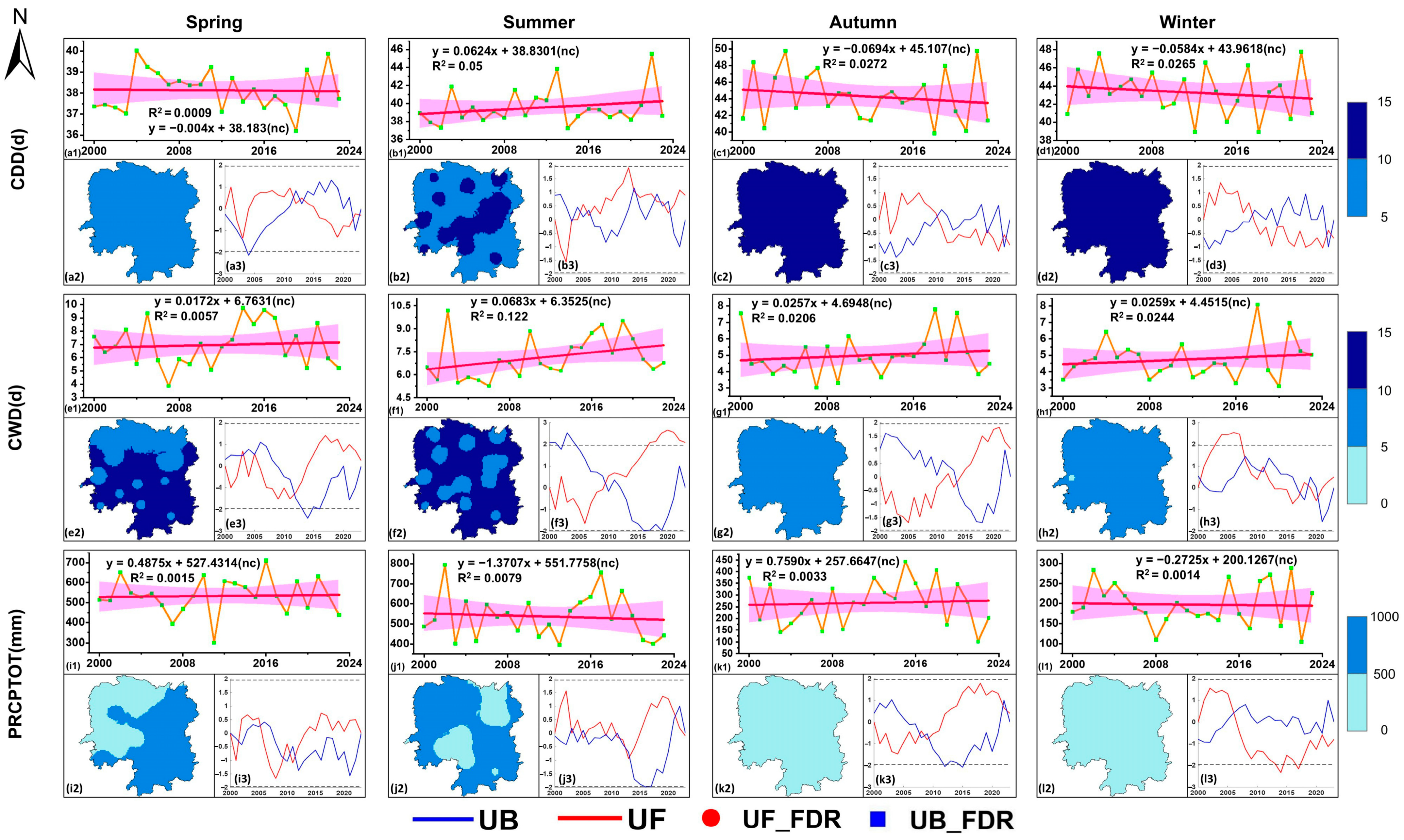
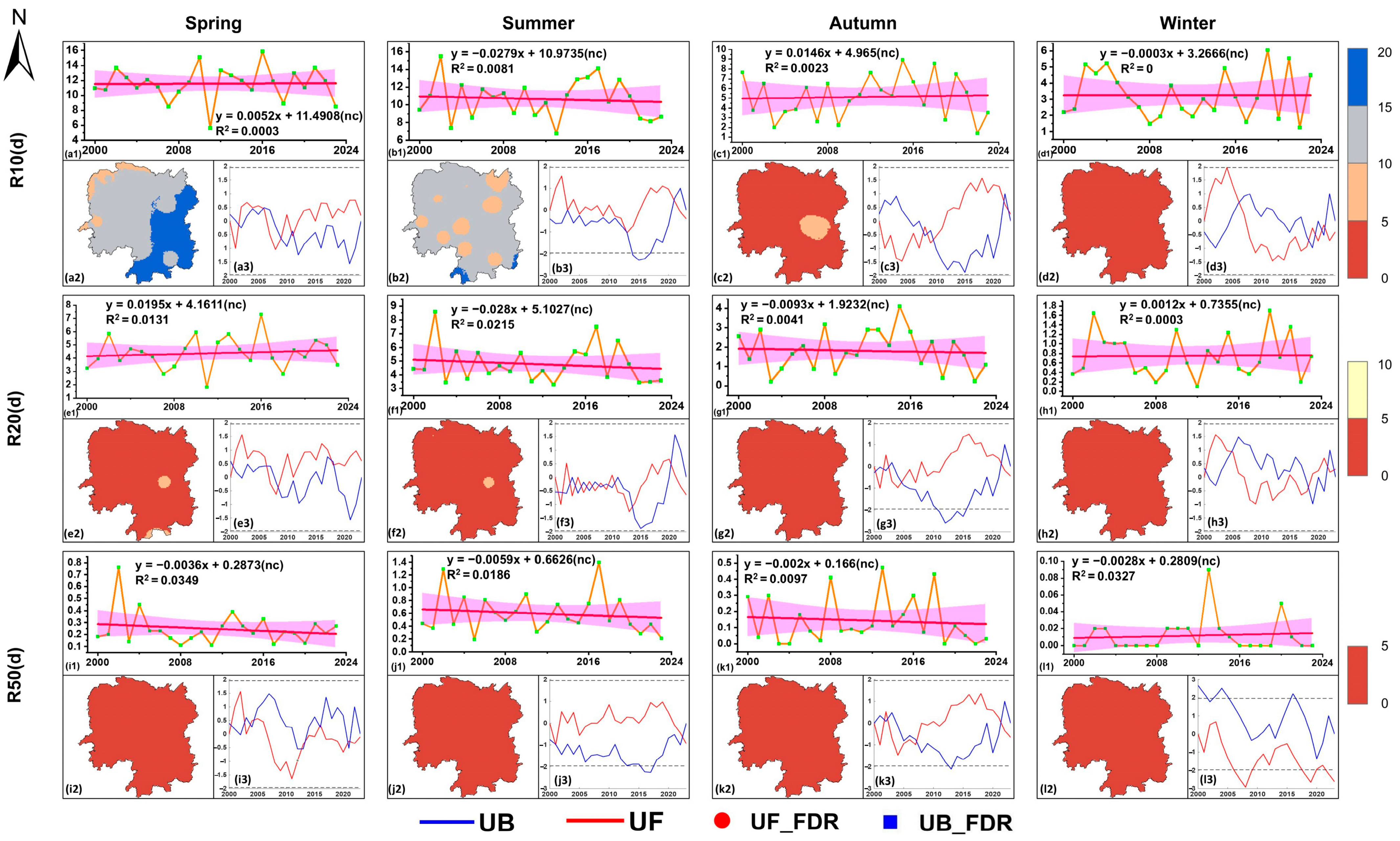
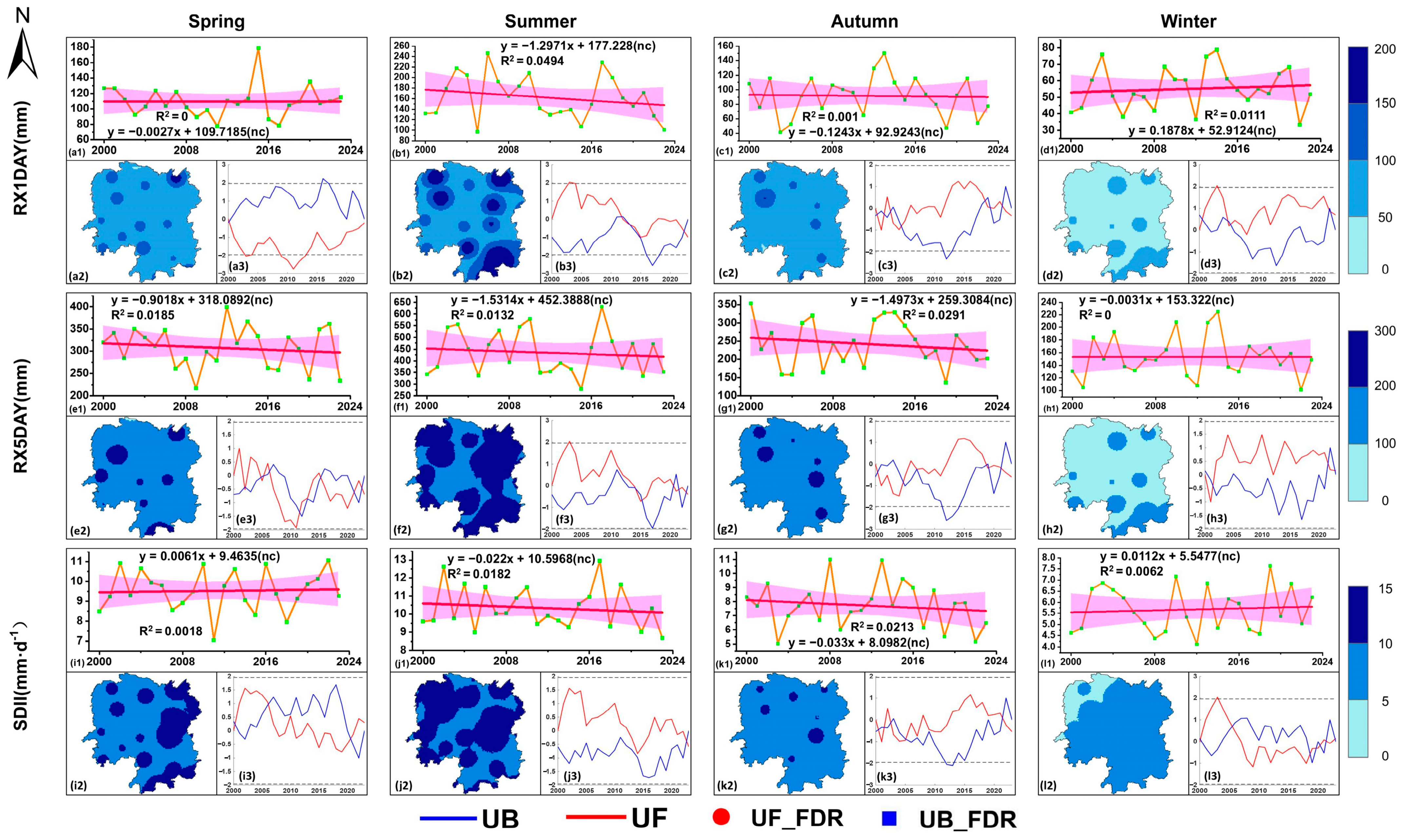
Based on the analysis results of 11 extreme precipitation indices in Hunan Province from 2000 to 2023, it can be seen that all kinds of extreme precipitation processes show obvious seasonal differences and regional inhomogeneity in time and space, but the overall trend is not significant. The linear fitting slope of each index was small; the coefficient of determination R² was generally lower than 0.05, and did not pass the significance test (nc). The Mann–Kendall (MK) trend test results further showed that the UF and UB curves of all indicators did not exceed the confidence interval (±1.96), and there was no obvious crossover point, indicating that there was no statistical mutation or trend transition in the extreme precipitation process in Hunan Province from 2000 to 2023. On the whole, the extreme precipitation showed fluctuating and stable temporal characteristics, and the spatial pattern remained stable, forming an overall distribution trend of “strong in the north and weak in the south, high in the west and low in the east”.

From the perspective of time variation characteristics, the interannual fluctuation range of consecutive dry days (CDDs) in each season is indeed limited. Taking spring as an example, its multi-year average state is about 38 days, the slope of the linear fitting equation is −0.004, and the coefficient of determination R² is as low as 0.0009, indicating that the downward trend is extremely weak and statistically insignificant. The CDDs in summer and winter showed a slight increase, with slopes of 0.0624 and 0.0683, respectively, but the corresponding R² was only 0.05 and 0.0272, which did not pass the significance test. The Mann–Kendall mutation test results further support the judgment of trend stability. The UF and UB statistics curves of all seasons are smoothly intertwined within the confidence interval, and there is no mutation point exceeding the critical value. At the same time, continuous wet days (CWDs) showed a relatively more obvious increasing trend in summer and autumn, with a slope of about 0.06–0.07. However, its determination coefficient was also at a low level and failed to constitute a statistically significant trend. The time series of seasonal total precipitation (PRCPTOT) is more stable. For example, the linear trend slope of autumn is only 0.0257 mm/year, and the UF and UB curves almost completely coincide, which systematically confirms that there has been no statistically significant trend change in total precipitation over the past two decades (Figure 2).

In terms of time variation characteristics, the number of days with annual precipitation ≥ 10 mm (R10) and ≥20 mm (R20) showed a high degree of stability throughout the study period. The slope value of the linear fitting trend line is extremely low, and the corresponding determination coefficient R² of each season is less than 0.03, which confirms that its trend with time is not statistically significant. The results of the Mann–Kendall mutation test were consistent with this. The UF and UB statistics curves of all seasons remained within the critical line of the significant level, and there was no clear crossover point across the critical value, indicating that there was no statistical mutation in the sequence. In contrast, the number of days with annual precipitation ≥ 50 mm (R50) showed a slight downward trend in most seasons, and the linear fitting slope was negative, ranging from −0.002 to −0.006 days/year. Although there is this tendency, the trend intensity is also weak, and R² in each season is lower than 0.04. The MK test curve further reveals the details of R50 changes. For example, in some seasons, the UF statistics may show a slight increase and then a decrease around 2010, but they have not broken through the significant boundary, which systematically confirms that although there are interannual fluctuations in the number of heavy precipitation days, the overall reduction trend is not statistically significant (Figure 3).

In the spatial distribution pattern, the chart shows that there are differences in the spatial patterns of precipitation days with different intensities. The distribution of R10 and R20 days in the whole province is relatively uniform, and there is no large-scale, continuous high-value or low-value concentration area. In contrast, the spatial heterogeneity of R50 days is more obvious, and its high value area is not concentrated and contiguous, but is distributed in a decentralized manner, mainly in the central and northern regions of Hunan Province. This spatial pattern indicates that the occurrence of extreme heavy precipitation days has stronger local characteristics.

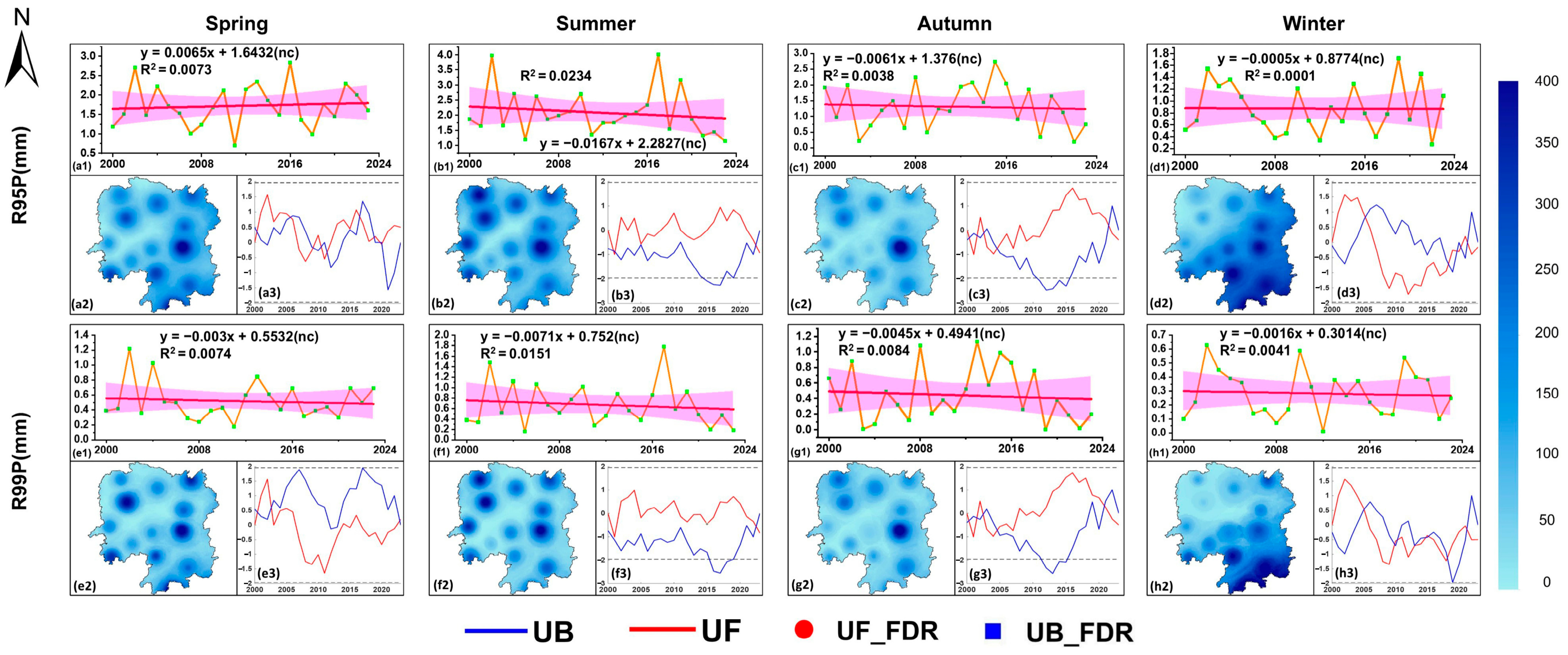
In terms of time trend, the heavy precipitation index R95P shows a weak seasonal difference. In spring, R95P showed a slight upward trend, and its linear fitting slope was +0.0065, but the explanatory power of this trend was very limited, and the coefficient of determination R² was only 0.0073. The R95P in summer and autumn turned to a slight decline, with slopes of −0.0061 and −0.0045, respectively, and the corresponding R² was also at a very low level (0.0038 and 0.0084, respectively), indicating that these trends were not statistically significant. For the extremely heavy precipitation index R99P, all seasons showed a consistent weak decreasing trend, and the linear fitting slope was between −0.0016 and −0.0071, among which the decreasing trend in summer was relatively obvious (slope was −0.0061, R² = 0.0234). Mann–Kendall mutation test results further support the conclusion that the trend is not significant. The UF and UB statistical curves of all seasonal series always fluctuate within the critical line of the significance level, and there is a significant intersection between the two, but it does not form a significant intersection beyond the confidence interval. Although there are some fluctuations in the curve during some periods (such as 2008–2015), the variation range is always controlled within the confidence interval, which systematically indicates that there is no statistical mutation in the extreme precipitation intensity during the study period (Figure 4).

In the spatial distribution pattern, R95P and R99P showed a highly consistent and stable spatial structure. The high-value areas are mainly concentrated in the central and northern plains of Hunan Province, while the low-value areas are stable in the hilly and mountainous areas in the south of Hunan and the south of the Yangtze River. This spatial distribution pattern of “high in the north-central and low in the south” clearly indicates that extreme precipitation events do not occur uniformly in space, but are relatively concentrated in the central and northern plains.

In terms of time trend, the maximum daily precipitation (RX1DAY) and the maximum five-day precipitation (RX5DAY) showed smooth fluctuations in each season, and did not show a significant linear trend. RX1DAY showed a weak downward trend in summer and autumn, and the linear fitting slopes were negative, but the trend intensity was extremely weak. The determination coefficient R² was lower than 0.05 (for example, R² = 0.001 for autumn RX1DAY), indicating that it was not statistically significant; the RX1DAY in spring and winter remained basically stable, and R² was close to 0.00. The change pattern of RX5DAY is similar. The downward trend in summer and autumn is relatively obvious. The linear fitting slope is about−1.5 mm/year, but its corresponding R² is also less than 0.05 (for example, R² = 0.0185 in spring RX5DAY), which does not reach the statistical significance level. The Mann–Kendall mutation test results are consistent with the above analysis. The UF and UB statistics curves of all seasonal series fluctuate within the confidence interval, and no crossover beyond the critical value occurs, which confirms that there is no significant mutation point during the study period. At the same time, the UF and UB curves of the precipitation intensity index (SDII) almost completely coincide and closely fit near the horizontal axis, which systematically confirms that the precipitation intensity of each season has remained highly stable over the past two decades, and no trend change or mutation signal has been detected (Figure 5).

In the spatial distribution pattern, the chart clearly shows the spatial differentiation characteristics of extreme precipitation. The high-value areas of the maximum daily precipitation (RX1DAY) and the maximum five-day precipitation (RX5DAY) (as shown in the blue scale) are significantly concentrated in the north-central and northwest regions of Hunan Province. For example, the high value of RX5DAY in summer can reach more than 500 mm, indicating that the region is the main place for short-term heavy rainfall and persistent extreme precipitation events. In contrast, other precipitation types are more dispersed.

3.2. Effects of Extreme Precipitation on Rice Yield in Hunan Province in This Study

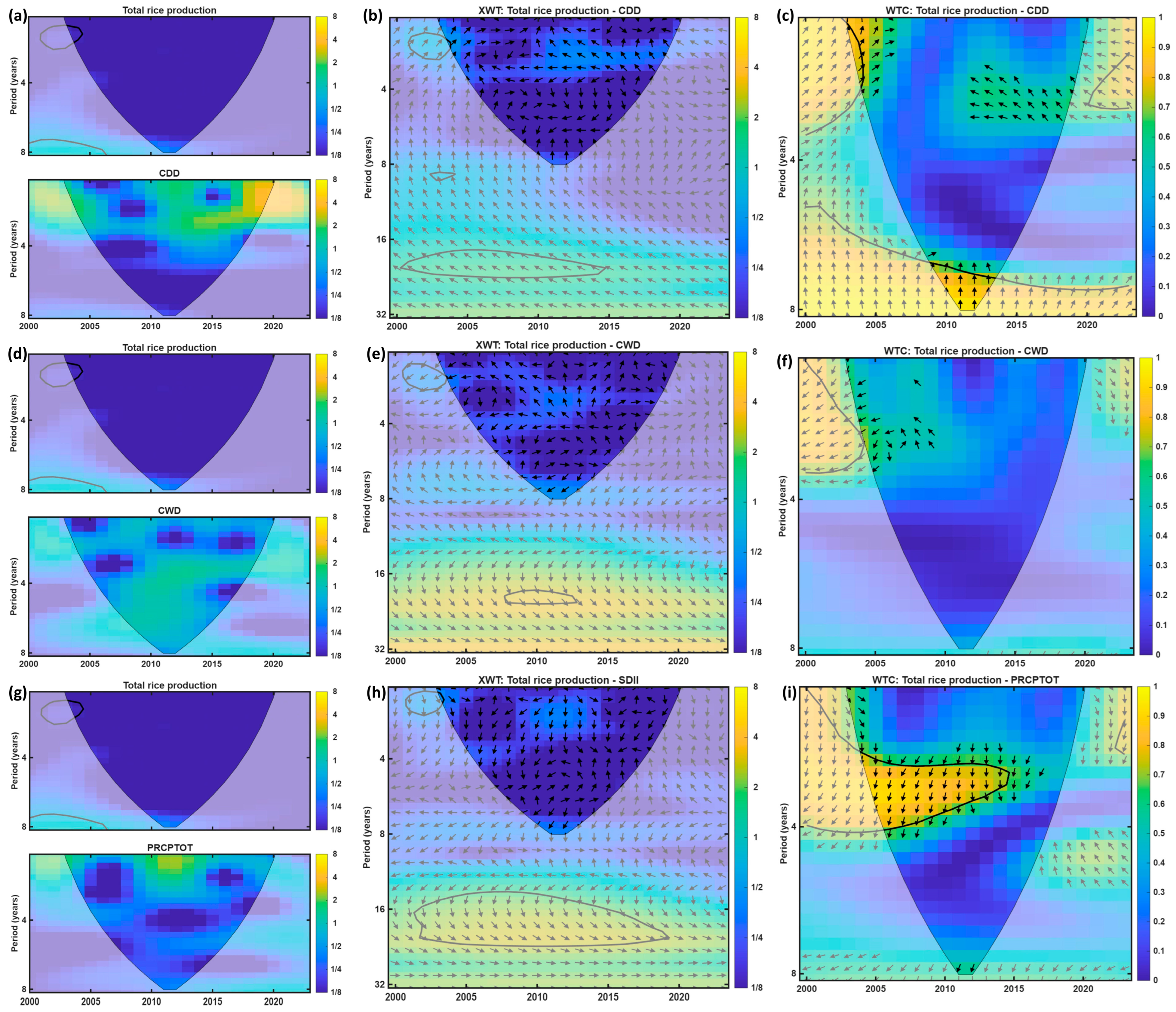
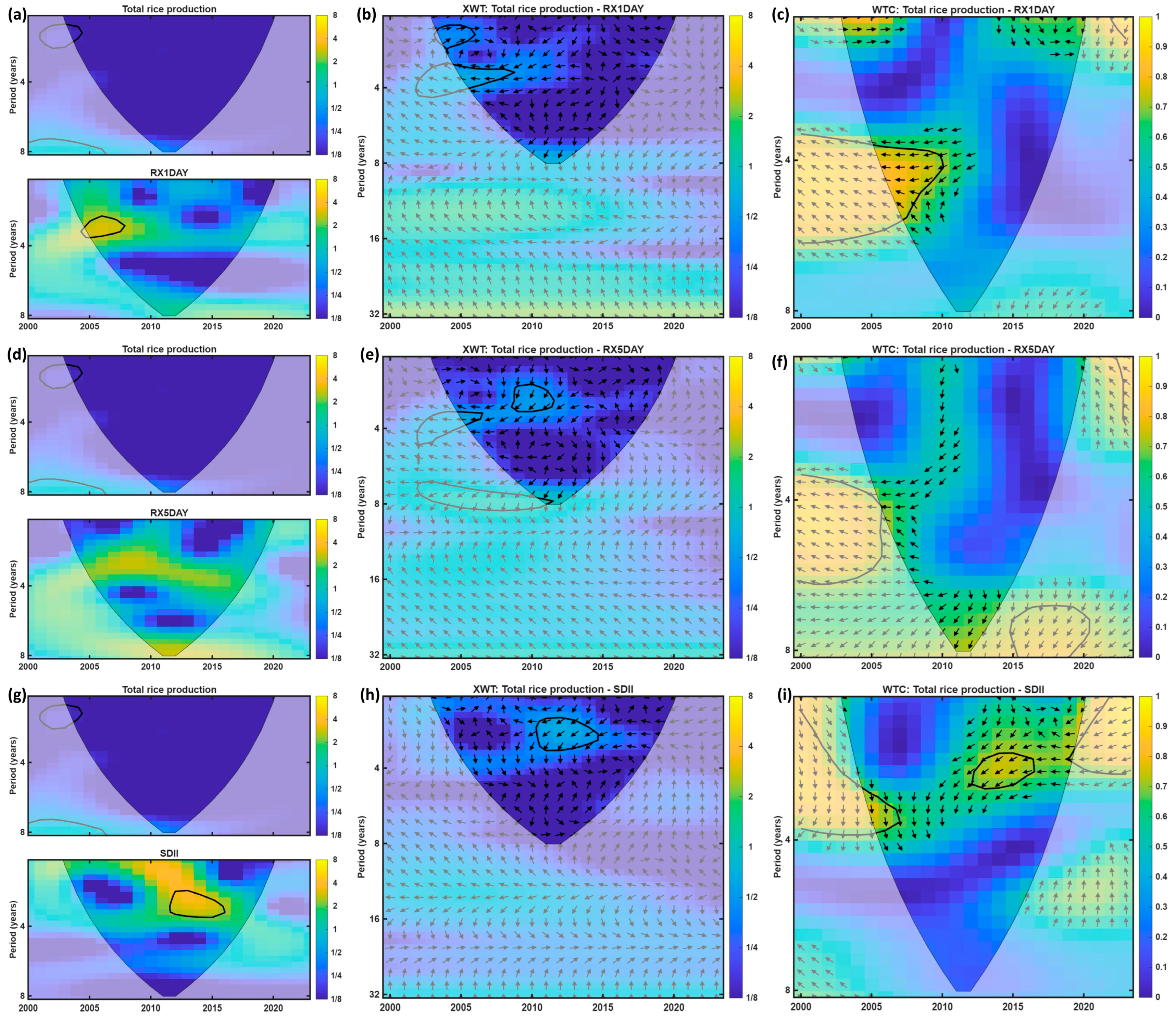
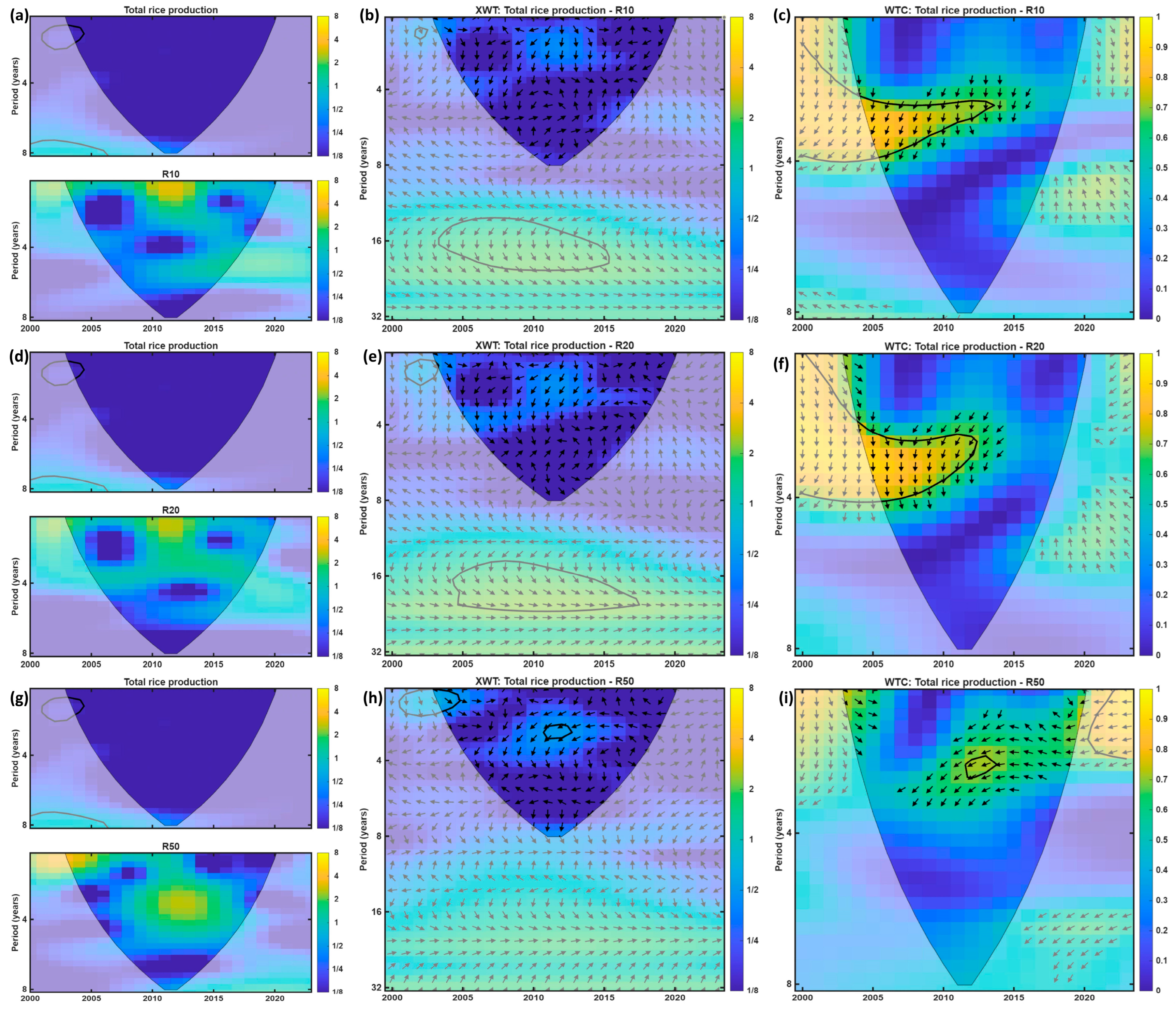
The Morlet mother wavelet is used for continuous wavelet transform (CWT), cross-wavelet spectral analysis (XWT), and wavelet coherence analysis (WTC). The central angular frequency is set to ω0 = 6 to ensure a good time–frequency resolution balance. The scale sequence is constructed according to the binary logarithmic interval, which can cover the typical climate cycle range of 2–32 years. The Monte Carlo random resampling method based on the AR (1) red noise background spectrum was used for the significance test, and the regions below the 95% significance level were drawn out with black solid coils. CWT reflects the periodic characteristics of the single sequence, XWT is used to identify the common high-energy region between the rice yield and extreme precipitation index, and WTC is used to evaluate the local coherence degree and the phase relationship between them.

The results of the wavelet analysis showed that there was a significant negative correlation between continuous drought days (CDDs) and rice yield in the 4–8-year cycle, especially in 2000–2005, and the persistence of drought showed obvious negative coherence (XWT diagram showed dark area). This result is consistent with Pearson correlation analysis (r = −0.38, p < 0.05), indicating that the inhibition of long-term drought on yield has a lag effect on the time scale (lag about 1–2 years). At the same time, the correlation of continuous wet days (CWDs) showed a positive relationship in the 8-year cycle, reflecting the promoting effect of the wet environment on rice yield. Especially during 2010–2015, wavelet analysis showed that the positive phase of the wet period was consistent with yield fluctuation, indicating that the wet period had a direct promoting effect on yield (right arrow in XWT). For the total precipitation (PRCPTOT), it showed a positive correlation (r = 0.29, p < 0.05) in a long period (about 4–8 years), which was consistent with the wavelet analysis, indicating that moderate precipitation contributed to the stable growth of rice (Figure 6).

Through XWT analysis, there was a significant negative correlation between R50 (number of days with daily precipitation ≥ 50 mm) and yield, especially during the period of 2008–2015; the lag effect of the heavy precipitation events on the yield was particularly prominent (XWT diagram shows dark areas and lag arrows), and this relationship was further confirmed by Pearson correlation (r = −0.44, p < 0.05). In contrast, the correlation between R10 (the number of days with precipitation ≥ 10 mm) and R20 (the number of days with precipitation ≥ 20 mm) is weak, and mainly concentrated in the short period (2–4 years), showing a lower negative impact. This indicates that the increase in the number of extreme precipitation days has a significant short-term effect on rice yield, while the number of days with less precipitation has a limited effect on yield (Figure 7).

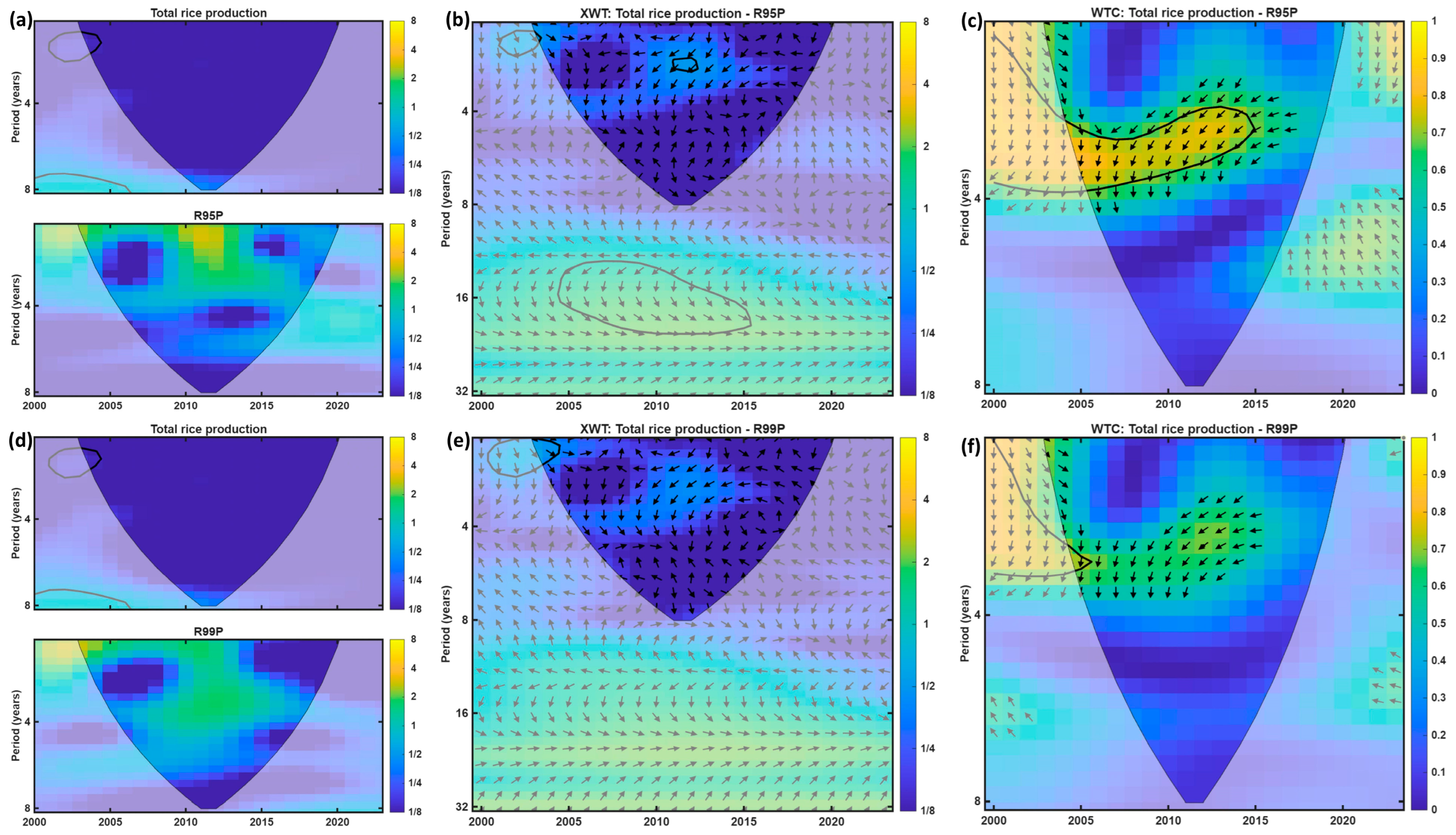
The analysis of R95P (the first 5% extreme precipitation events) and R99P (the first 1% extreme precipitation events) showed that the impact of these extreme precipitation events on rice yield was particularly prominent in the lag period. The wavelet analysis showed that the phase relationship between R99P and rice yield gradually showed a strong negative correlation between 2010 and 2020 (the arrows in the XWT diagram were shifted to the right), indicating that the lag inhibitory effect of extreme precipitation on yield became more obvious during this period (r = −0.42, p < 0.05). This result is consistent with Pearson correlation analysis, indicating that the long-term impact of frequent extreme precipitation events on yield is intensifying (Figure 8).

In the wavelet analysis, the correlation between the daily maximum precipitation (RX1DAY) and the five-day maximum precipitation (RX5DAY) on rice yield showed a significant negative correlation in the 4–8-year cycle, especially in the period of 2000–2023, and the lag effect is obvious (XWT dark area). The precipitation intensity index (SDII) showed a short-term positive correlation (0.5–2-year cycle), especially in 2010–2015; the immediate impact of precipitation intensity on yield fluctuations was particularly prominent (r = 0.35, p < 0.05). Wavelet analysis further confirmed this, indicating that the increase in extreme precipitation intensity events had an immediate promoting effect on rice yield (Figure 9).

4. Discussion

4.1. Extreme Precipitation Pattern and Its Coupling Background with Rice Production in Hunan Province

The sensitivity of rice systems to extreme precipitation has received increasing attention worldwide [72,73]. Evidence for China indicates that extreme rainfall has reduced national rice yield over recent decades [73]. In southern China, frequent and intense heavy rainfall may influence rice yield through both immediate damage and lagged effects, including nutrient loss and root hypoxia [74,75].

This study shows that extreme precipitation in Hunan Province during 2000–2023 is overall stable in trend, but highly concentrated in time and space. This “stable baseline with concentrated extremes” implies that rice production can remain relatively resilient under current conditions, likely supported by the local double-cropping system and management improvements [76,77]. However, resilience under today’s baseline does not eliminate future risks, especially when extremes overlap with sensitive growth stages.

Mechanistically, heavy rainfall impacts rice via two main pathways. The first is immediate impacts, such as lodging, panicle damage, and delayed grain filling, which have been reported in field and experimental studies [78,79,80]. The second is a delayed response pathway, where post-event water retention and slow drainage can lead to prolonged root oxygen deficiency and subsequent yield penalties [80,81]. Consistent with this, our wavelet results indicate that, within the 4–8-year high-energy coupling band, precipitation anomalies tend to lead yield variability by about 1–2 years, supporting a lagged response signal [82,83].

Although no significant linear trend is detected in Hunan’s extreme precipitation over 2000–2023, multi-model projections under the East Asian summer monsoon background suggest that short-duration high-intensity precipitation may increase in both frequency and intensity [84,85]. In addition, compound extremes relevant to rice production are increasingly discussed in South China, and severe convection-related events are also notable in Hunan [86,87]. Given Hunan’s complex terrain and lake–plain–hill mosaic, exposure and waterlogging risk are spatially heterogeneous [88,89], and regional differentiation in precipitation-related impacts is widely recognized [90,91,92]. Therefore, risk management should focus not only on mean-state stability but also on threshold exceedance and spatial hotspots.

4.2. Horizontal Comparison with Grain Producing Areas in North China and the Middle and Lower Reaches of the Yangtze River

A comparison with winter wheat regions highlights crop- and region-specific sensitivity to precipitation extremes. Studies report substantial winter wheat yield losses under waterlogging in major grain areas (e.g., Henan) [93,94], and satellite-based assessments also confirm strong waterlogging-related yield impacts in the middle and lower Yangtze River wheat region [95]. In contrast, rice in Hunan does not show significant yield reduction in years with higher extreme precipitation indices, indicating a higher tolerance threshold under comparable extreme intensity categories.

This difference is consistent with the physiological and ecological traits of rice. Rice can better tolerate short-term ponding due to its semi-aquatic adaptations (e.g., aerenchyma formation and anaerobic metabolism), which help maintain function under temporary waterlogging [96,97,98]. However, tolerance is not unlimited: prolonged flooding/submergence can sharply suppress photosynthesis and accelerate yield loss [99]. For wheat, critical-stage waterlogging (e.g., near anthesis) is widely reported to be highly damaging [100,101,102,103]. Overall, these comparisons support a nonlinear, threshold-like response rather than a simple linear accumulation of precipitation impacts, and emphasize the need for crop-specific warning thresholds under increasingly rare and intense events [104,105,106].

4.3. Climate Adaptation Strategies and Policy Implications

Given the potential risk from extreme precipitation, adaptation in Hunan should target the risk chain “heavy rainfall → waterlogging exposure and recovery delay → yield volatility (including lagged effects)”. At the governance and investment level, research on high-standard farmland and related policy impacts supports the importance of strengthening field infrastructure and management capacity [107,108,109,110,111,112,113,114]. At the household level, evidence from Hunan indicates that natural hazards influence agricultural decision-making, supporting the need for practical and timely services [115,116,117].

Three directions are most actionable. First, in the operational dimension, improve rapid drainage and post-event recovery capacity, including coordinated machinery and service response, which is crucial for preventing short-term ponding from turning into damaging waterlogging [81,118,119,120,121,122,123,124,125,126]. Second, in the technical dimension, strengthen agrometeorological and hydrological monitoring and early warnings, and translate forecasts into field-level guidance. The demonstrated lagged relationships between precipitation and soil moisture anomalies and the progress in remote sensing-based flood/waterlogging monitoring provide feasible technical support for earlier interventions [127,128,129,130,131,132,133,134]. Third, in the institutional dimension, improve risk-compensation and insurance mechanisms and explore index-triggered designs (e.g., weather/yield triggers) to shorten the response delays when extreme indices exceed thresholds [85,135,136,137,138,139,140]. More broadly, adaptive governance approaches and climate-smart agriculture frameworks provide directions for integrating finance, services, and technology into resilience building [141,142,143,144,145,146]. In practice, thresholds should be calibrated to local drainage capacity and spatial heterogeneity to ensure feasibility and effectiveness [85,147].

5. Conclusions

From 2000 to 2023, extreme precipitation in Hunan Province exhibited fluctuating stability with no significant trends in major indices (RX1DAY, RX5DAY, R95P, R99P, CWD, PRCPTOT), as confirmed by Mann–Kendall tests. Spatially, extremes concentrated in the central Dongting Lake Plain and surrounding hills with high intensity, while southern mountainous areas showed high frequency but low intensity. Seasonal concentration in June–August aligned with East Asian monsoon activity, characterizing an “overall stability–seasonal concentration–spatial inequality” pattern.

Rice yield displayed a “core–transition–marginal” gradient differentiation. Core production zones (central Hunan, Dongting Lake Plain) achieved steady yield gains; transition zones (southern hills, western low mountains) showed high volatility; marginal areas experienced continuous decline in both acreage and yield, forming a “core stability–transition fluctuation–marginal contraction” pattern.

Extreme precipitation’s impacts on rice yield were multi-scale, lagged, and region-specific. Significant negative correlations occurred at 4–8-year cycles (e.g., R50 vs. yield r = −0.44) with 1–2-year lags; short-cycle (0.5–2-year) precipitation intensity (SDII) synchronized with yield $\mathrm{r}=0.35$. Core zones demonstrated strong flood resistance due to adequate drainage, while transition zones showed the highest correlation and sensitivity. The relationship was nonlinear–threshold: moderate wetting stabilized yields, but intensity/duration exceeding ecological thresholds caused sharp declines.

Based on these findings, climate adaptation strategies include the following: (1) Enhancing high-standard farmland “storage–drainage–infiltration–retardation” coordination; (2) Building multi-threshold precipitation monitoring and early-warning systems; (3) Promoting waterlogging-tolerant varieties and optimizing sowing dates; (4) Establishing “threshold-triggered” insurance compensation mechanisms.

References

1. Arias, P.; Bellouin, N.; Coppola, E.; Jones, R.; Krinner, G.; Marotzke, J.; Naik, V.; Palmer, M.; Plattner, G.-K.; Rogelj, J.; et al. Climate Change 2021: The Physical Science Basis. Working Group I Contribution to the Sixth Assessment Report of the Intergovernmental Panel on Climate Change. Available online: https://www.ipcc.ch/report/ar6/wg1/downloads/report/IPCC_AR6_WGI_FullReport.pdf (accessed on 17 June 2025).
2. Alexander, L.V.; Zhang, X.; Peterson, T.C.; Caesar, J.; Gleason, B.; Klein Tank, A.M.G.; Haylock, M.; Collins, D.; Trewin, B.; Rahimzadeh, F.; et al. Global observed changes in daily climate extremes of temperature and precipitation. J. Geophys. Res. Atmos. 2006, 111. [Google Scholar] [CrossRef]
3. Lesk, C.; Rowhani, P.; Ramankutty, N. Influence of extreme weather disasters on global crop production. Nature 2016, 529, 84–87. [Google Scholar] [CrossRef]
4. Donat, M.G.; Lowry, A.L.; Alexander, L.V.; O’Gorman, P.A.; Maher, N. More extreme precipitation in the world’s dry and wet regions. Nat. Clim. Change 2016, 6, 508–513. [Google Scholar] [CrossRef]
5. Zhang, B.; Song, S.; Wang, H.; Guo, T.; Ding, Y. Evaluation of the performance of CMIP6 models in simulating extreme precipitation and its projected changes in global climate regions. Nat. Hazards 2025, 121, 1737–1763. [Google Scholar] [CrossRef]
6. He, S.; Takemi, T. Future Changes of Extreme Precipitation and Related Atmospheric Conditions in East Asia under Global Warming Projected in Large Ensemble Climate Prediction Data. J. Clim. 2024, 37, 5171–5186. [Google Scholar] [CrossRef]
7. Zeng, X.; Li, Z.; Zeng, F.; Caputo, F.; Chin, T. Spatiotemporal evolution and antecedents of rice production efficiency: From a geospatial approach. Systems 2023, 11, 131. [Google Scholar] [CrossRef]
8. Zeng, Y.; Huang, C.; Tang, Y.; Peng, J. Precipitation variations in the flood seasons of 1910–2019 in hunan and its association with the PDO, AMO, and ENSO. Front. Earth Sci. 2021, 9, 656594. [Google Scholar] [CrossRef]
9. Hu, X.; Wang, M.; Liu, K.; Gong, D.; Kantz, H. Using climate factors to estimate flood economic loss risk. Int. J. Disaster Risk Sci. 2021, 12, 731–744. [Google Scholar] [CrossRef]
10. Sun, S.; Zhao, Y.; He, Y.; Xia, Z.; Chen, S.; Zhang, Y.; Sun, Q. Exacerbated climate risks induced by precipitation extremes in the Yangtze River basin under warming scenarios. Front. Ecol. Evol. 2023, 11, 1127875. [Google Scholar] [CrossRef]
11. Shi, W.; Wang, M.; Liu, Y. Crop yield and production responses to climate disasters in China. Sci. Total Environ. 2021, 750, 141147. [Google Scholar] [CrossRef]
12. Liu, W.; Sun, W.; Huang, J.; Wen, H.; Huang, R. Excessive rainfall is the key meteorological limiting factor for winter wheat yield in the middle and lower reaches of the Yangtze River. Agronomy 2021, 12, 50. [Google Scholar] [CrossRef]
13. Wang, C.; Zhang, Z.; Zhang, J.; Tao, F.; Chen, Y.; Ding, H. The effect of terrain factors on rice production: A case study in Hunan Province. J. Geogr. Sci. 2019, 29, 287–305. [Google Scholar] [CrossRef]
14. Lipper, L.; Thornton, P.; Campbell, B.M.; Baedeker, T.; Braimoh, A.; Bwalya, M.; Caron, P.; Cattaneo, A.; Garrity, D.; Henry, K.; et al. Climate-smart agriculture for food security. Nat. Clim. Change 2014, 4, 1068–1072. [Google Scholar] [CrossRef]
15. Lobell, D.B.; Schlenker, W.; Costa-Roberts, J. Climate trends and global crop production since 1980. Science 2011, 333, 616–620. [Google Scholar] [CrossRef]
16. Auffhammer, M.; Hsiang, S.M.; Schlenker, W.; Sobel, A. Using weather data and climate model output in economic analyses of climate change. Rev. Environ. Econ. Policy 2013, 7, 181–198. [Google Scholar] [CrossRef]
17. Rosenzweig, C.; Elliott, J.; Deryng, D.; Ruane, A.C.; Müller, C.; Arneth, A.; Folberth, C.; Glotter, M.; Khabarov, N.; Neumann, K.; et al. Assessing agricultural risks of climate change in the 21st century in a global gridded crop model intercomparison. Proc. Natl. Acad. Sci. USA 2014, 111, 3268–3273. [Google Scholar] [CrossRef]
18. Burke, M.; Hsiang, S.M.; Miguel, E. Global non-linear effect of temperature on economic production. Nature 2015, 527, 235–239. [Google Scholar] [CrossRef]
19. Howden, S.M.; Soussana, J.F.; Tubiello, F.N.; Chhetri, N.; Dunlop, M.; Meinke, H. Adapting agriculture to climate change. Proc. Natl. Acad. Sci. USA 2007, 104, 19691–19696. [Google Scholar] [CrossRef] [PubMed]
20. Phukan, U.J.; Jindal, S.; Laldinsangi, C.; Singh, P.K.; Longchar, B. A microscopic scenario on recovery mechanisms under waterlogging and submergence stress in rice. Planta 2024, 259, 9. [Google Scholar] [CrossRef]
21. Carleton, T.A.; Hsiang, S.M. Social and economic impacts of climate. Science 2016, 353, aad9837. [Google Scholar] [CrossRef]
22. Lobell, D.B.; Hammer, G.L.; McLean, G.; Messina, C.; Roberts, M.J.; Schlenker, W. The critical role of extreme heat for maize production in the United States. Nat. Clim. Change 2013, 3, 497–501. [Google Scholar] [CrossRef]
23. Dell, M.; Jones, B.F.; Olken, B.A. What do we learn from the weather? The new climate-economy literature. J. Econ. Lit. 2014, 52, 740–798. [Google Scholar] [CrossRef]
24. Doi, T.; Sakurai, G.; Iizumi, T. Seasonal predictability of four major crop yields worldwide by a hybrid system of dynamical climate prediction and eco-physiological crop-growth simulation. Front. Sustain. Food Syst. 2020, 4, 84. [Google Scholar] [CrossRef]
25. Knox, J.; Hess, T.; Daccache, A.; Wheeler, T. Climate change impacts on crop productivity in Africa and South Asia. Environ. Res. Lett. 2012, 7, 034032. [Google Scholar] [CrossRef]
26. Deschênes, O.; Greenstone, M. The economic impacts of climate change: Evidence from agricultural output and random fluctuations in weather. Am. Econ. Rev. 2007, 97, 354–385. [Google Scholar] [CrossRef]
27. Diffenbaugh, N.S.; Hertel, T.W.; Scherer, M.; Verma, M. Response of corn markets to climate volatility under alternative energy futures. Nat. Clim. Change 2012, 2, 514–518. [Google Scholar] [CrossRef] [PubMed]
28. Zhang, J.; Zhang, Z.; Wang, C.; Tao, F. Double-rice system simulation in a topographically diverse region—A remote-sensing-driven case study in Hunan Province of China. Remote Sens. 2019, 11, 1577. [Google Scholar] [CrossRef]
29. Mendelsohn, R. (Ed.) Agriculture: A Ricardian Analysis; Edward Elgar Publishing: Cheltenham, UK, 2001; pp. 32–53. [Google Scholar]
30. Jägermeyr, J.; Müller, C.; Ruane, A.C.; Elliott, J.; Balkovic, J.; Castillo, O.; Foster, I.; Folberth, C.; Franke, J.A.; Fuchs, K.; et al. Climate impacts on global agriculture emerge earlier in new generation of climate and crop models. Nat. Food 2021, 2, 873–885. [Google Scholar] [CrossRef] [PubMed]
31. Moore, F.C.; Baldos, U.; Hertel, T.; Diaz, D. New science of climate change impacts on agriculture implies higher social cost of carbon. Nat. Commun. 2017, 8, 1607. [Google Scholar] [CrossRef] [PubMed]
32. Ortiz-Bobea, A.; Ault, T.R.; Carrillo, C.M.; Chambers, R.G.; Lobell, D.B. Anthropogenic climate change has slowed global agricultural productivity growth. Nat. Clim. Change 2021, 11, 306–312. [Google Scholar] [CrossRef]
33. Porter, J.; Xie, L.; Challinor, A.J.; Howden, M.; Iqbal, M.M.; Lobell, D.B.; Travasso, M.I. Food Security and Food Production Systems; Cambridge University Press: Cambridge, UK, 2014. [Google Scholar]
34. Schmidhuber, J.; Tubiello, F.N. Global food security under climate change. Proc. Natl. Acad. Sci. USA 2007, 104, 19703–19708. [Google Scholar] [CrossRef] [PubMed]
35. Li, M.F.; Luo, W.; Li, H.; Liu, E.; Li, Y. Daily extreme precipitation indices and their impacts on rice yield—A case study over the tropical island in China. Theor. Appl. Climatol. 2018, 132, 503–513. [Google Scholar] [CrossRef]
36. Abramoff, R.Z.; Ciais, P.; Zhu, P.; Hasegawa, T.; Wakatsuki, H.; Makowski, M. Adaptation strategies strongly reduce the future impacts of climate change on simulated crop yields. Earth’s Future 2023, 11, e2022EF003190. [Google Scholar] [CrossRef]
37. Tack, J.; Barkley, A.; Nalley, L.L. Effect of warming temperatures on US wheat yields. Proc. Natl. Acad. Sci. USA 2015, 112, 6931–6936. [Google Scholar] [CrossRef] [PubMed]
38. Huang, J.; Islam, A.T.; Zhang, F.; Hu, Z. Spatiotemporal analysis the precipitation extremes affecting rice yield in Jiangsu province, southeast China. Int. J. Biometeorol. 2017, 61, 1863–1872. [Google Scholar] [CrossRef]
39. Deng, Q.; Xie, W.; Wang, K. Impact of extreme temperatures on production of different rice types: A county-level analysis for China. Appl. Econ. Perspect. Policy 2023, 45, 1097–1133. [Google Scholar] [CrossRef]
40. Menne, M.J.; Durre, I.; Vose, R.S.; Gleason, B.E.; Houston, T.G. An overview of the global historical climatology network-daily database. J. Atmos. Ocean. Technol. 2012, 29, 897–910. [Google Scholar] [CrossRef]
41. Durre, I.; Menne, M.J.; Gleason, B.E.; Houston, T.G.; Vose, R. Comprehensive automated quality assurance of daily surface observations. J. Appl. Meteorol. Climatol. 2010, 49, 1615–1631. [Google Scholar]
42. Donat, M.G.; Alexander, L.V.; Yang, H.; Durre, I.; Vose, R.; Caesar, J. Global land-based datasets for monitoring climatic extremes. Bull. Am. Meteorol. Soc. 2013, 94, 997–1006. [Google Scholar] [CrossRef]
43. Huang, B.; Wang, Z.; Yin, X.; Arguez, A.; Graham, G.; Liu, C.; Smith, T.; Zhang, H.M. Prolonged marine heatwaves in the Arctic: 1982−2020. Geophys. Res. Lett. 2021, 48, e2021GL095590. [Google Scholar] [CrossRef]
44. Stojanovski, P.; Dong, W.; Wang, M.; Ye, T.; Li, S.; Mortgat, C.P. Agricultural risk modeling challenges in China: Probabilistic modeling of rice losses in Hunan Province. Int. J. Disaster Risk Sci. 2015, 6, 335–346. [Google Scholar] [CrossRef]
45. Yu, D.; Hu, S.; Tong, L.; Xia, C.; Ran, P. Dynamics and determinants of the grain yield gap in major grain-producing areas: A case study in Hunan Province, China. Foods 2022, 11, 1122. [Google Scholar] [CrossRef] [PubMed]
46. Huang, K.; Tang, W.; Zhou, F. Agricultural Productive Services and Ecological Efficiency of Cultivated Land Use: Evidence from Hunan Province, China. Pol. J. Environ. Stud. 2024, 33, 5127–5140. [Google Scholar] [CrossRef]
47. Li, S.; Luo, H. Competitiveness of Rice Industry in Hunan Province—A Diamond Model. In Proceedings of the IOP Conference Series: Earth and Environmental Science, Paris, France, 7–9 November 2018; IOP Publishing: Bristol, UK, 2018; Volume 189, p. 042005. [Google Scholar]
48. Huang, G.; Wen, G. Spatial and temporal variations of light rain events over China and the mid-high latitudes of the Northern Hemisphere. Chin. Sci. Bull. 2013, 58, 1402–1411. [Google Scholar] [CrossRef]
49. Groisman, P.Y.; Knight, R.W.; Zolina, O.G. Recent trends in regional and global intense precipitation patterns. Clim. Vulnerability 2013, 5, 25–55. [Google Scholar]
50. Chen, X.; Wang, H.; Lyu, W.; Xu, R. The Mann-Kendall-Sneyers test to identify the change points of COVID-19 time series in the United States. BMC Med. Res. Methodol. 2022, 22, 233. [Google Scholar] [CrossRef]
51. Nicolakopoulos, S.; Cator, E.; Janssen, M.P. Extending the Mann–Kendall test to allow for measurement uncertainty. Statistics 2023, 57, 577–596. [Google Scholar] [CrossRef]
52. Collaud Coen, M.; Andrews, E.; Bigi, A.; Martucci, G.; Romanens, G.; Vogt, F.P.; Vuilleumier, L. Effects of the prewhitening method, the time granularity, and the time segmentation on the Mann–Kendall trend detection and the associated Sen’s slope. Atmos. Meas. Tech. 2020, 13, 6945–6964. [Google Scholar] [CrossRef]
53. Armstrong, T.B. False discovery rate adjustments for average significance level controlling tests. arXiv 2022, arXiv:2209.13686. [Google Scholar] [CrossRef]
54. Yang, L.; Wang, P.; Chen, J. 2dGBH: Two-dimensional group Benjamini–Hochberg procedure for false discovery rate control in two-way multiple testing of genomic data. Bioinformatics 2024, 40, btae035. [Google Scholar] [CrossRef]
55. Pournaderi, M.; Xiang, Y. Communication-efficient distributed multiple testing for large-scale inference. In Proceedings of the 2022 IEEE International Symposium on Information Theory (ISIT), Espoo, Finland, 26 June–1 July 2022; IEEE: New York, NY, USA, 2022; pp. 1477–1482. [Google Scholar]
56. Zhou, H.; Zhu, J.; Xiao, H.; Wang, X. Singular value decomposition (SVD) based correlation analysis of climatic factors and extreme precipitation in Hunan Province, China, during 1960–2009. J. Water Clim. Change 2021, 12, 3602–3616. [Google Scholar] [CrossRef]
57. Dunn, R.J.; Donat, M.G.; Alexander, L.V. Comparing extremes indices in recent observational and reanalysis products. Front. Clim. 2022, 4, 989505. [Google Scholar] [CrossRef]
58. Liu, S.; Chang, G. Spatial-temporal analysis of precipitation extremes over China during 1961–2019. Discov. Atmos. 2025, 3, 24. [Google Scholar] [CrossRef]
59. Addou, R.; Hanchane, M.; Krakauer, N.Y.; Kessabi, R.; Obda, K.; Souab, M.; Achir, I.E. Wavelet analysis for studying rainfall variability and regionalizing data: An applied study of the Moulouya watershed in Morocco. Appl. Sci. 2023, 13, 3841. [Google Scholar] [CrossRef]
60. Ahmadi, F.; Mirabbasi, R.; Kumar, R.; Gajbhiye, S. Prediction of precipitation using wavelet-based hybrid models considering the periodicity. Neural Comput. Appl. 2024, 36, 16345–16364. [Google Scholar] [CrossRef]
61. Khan, A.; Hassan, D.; Raza, S.M.M.; Amjad, M.; Mian, K. Applications of wavelet transform in climatic time series: A case study of Gilgit-Baltistan, Pakistan. Int. J. Environ. Sci. Technol. 2025, 22, 13749–13768. [Google Scholar] [CrossRef]
62. Hu, W.; Si, B. Improved partial wavelet coherency for understanding scale-specific and localized bivariate relationships in geosciences. Hydrol. Earth Syst. Sci. 2021, 25, 321–331. [Google Scholar] [CrossRef]
63. Alsubih, M.; Mallick, J.; Alqadhi, S.; Hang, H.T. Spatiotemporal analysis of drought severity and vegetation health using wavelet coherence: A case study in arid regions of Saudi Arabia. Theor. Appl. Climatol. 2025, 156, 1–32. [Google Scholar] [CrossRef]
64. Grinsted, A.; Moore, J.C.; Jevrejeva, S. Application of the cross wavelet transform and wavelet coherence to geophysical time series. Nonlinear Process. Geophys. 2004, 11, 561–566. [Google Scholar] [CrossRef]
65. Maraun, D.; Kurths, J. Cross wavelet analysis: Significance testing and pitfalls. Nonlinear Process. Geophys. 2004, 11, 505–514. [Google Scholar] [CrossRef]
66. Torrence, C.; Compo, G.P. A practical guide to wavelet analysis. Bull. Am. Meteorol. Soc. 1998, 79, 61–78. [Google Scholar] [CrossRef]
67. Torrence, C.; Webster, P.J. Interdecadal changes in the ENSO–monsoon system. J. Clim. 1999, 12, 2679–2690. [Google Scholar]
68. Magnello, M.E. Karl Pearson and the origins of modern statistics: An elastician becomes a statistician. New Zealand J. Hist. Philos. Sci. Technol. 2005, 1, 010107. [Google Scholar]
69. Cohen, J.; Cohen, P.; West, S.G.; Aiken, L.S. Applied Multiple Regression/Correlation Analysis for the Behavioral Sciences; Routledge: Abingdon, UK, 2013. [Google Scholar]
70. Pearson, K., VII. Mathematical contributions to the theory of evolution.—III. Regression, heredity, and panmixia. Philos. Trans. A Math. Phys. Eng. Sci. 1896, 253–318. [Google Scholar] [CrossRef]
71. Lee Rodgers, J.; Nicewander, W.A. Thirteen ways to look at the correlation coefficient. Am. Stat. 1988, 42, 59–71. [Google Scholar] [CrossRef]
72. Zhao, W.; Chou, J.; Li, J.; Xu, Y.; Li, Y.; Hao, Y. Impacts of extreme climate events on future rice yields in global major rice-producing regions. Int. J. Environ. Res. Public Health 2022, 19, 4437. [Google Scholar] [CrossRef]
73. Fu, J.; Jian, Y.; Wang, X.; Li, L.; Ciais, P.; Zscheischler, J.; Wang, Y.; Tang, Y.; Müller, C.; Webber, H.; et al. Extreme rainfall reduces one-twelfth of China’s rice yield over the last two decades. Nat. Food 2023, 4, 416–426. [Google Scholar] [CrossRef] [PubMed]
74. Aslam, A.; Mahmood, A.; Ur-Rehman, H.; Li, C.; Liang, X.; Shao, J.; Negm, S.; Moustafa, M.; Aamer, M.; Hassan, M.U. Plant Adaptation to Flooding Stress under Changing Climate Conditions: Ongoing Breakthroughs and Future Challenges. Plants 2023, 12, 3824. [Google Scholar] [CrossRef] [PubMed]
75. Jian, Y.; Fu, J.; Zhou, F. A review of studies on the impacts of extreme precipitation on rice yields. Prog. Geogr. 2021, 40, 1746–1760. [Google Scholar] [CrossRef]
76. Li, S.; Shi, X.; Lu, J.; Chen, F.; Chu, Q. Climate warming and crop management: A comprehensive analysis of changes on distribution of suitable areas for double rice. Agronomy 2022, 12, 993. [Google Scholar] [CrossRef]
77. Wang, X.; Han, J.; Li, R.; Qiu, L.; Zhang, C.; Lu, M.; Huang, R.; Wang, X.; Ouyang, X. Gradual daylength sensing coupled with optimum cropping modes enhances multi-latitude adaptation of rice and maize. Plant Commun. 2023, 4, 100433. [Google Scholar] [CrossRef]
78. Agusta, H.; Santosa, E.; Dulbari, D.; Guntoro, D.; Zaman, S. Continuous heavy rainfall and wind velocity during flowering affect rice production. Agrivita J. Agric. Sci. 2022, 44, 290–302. [Google Scholar]
79. Ohe, M.; Matsuo, H. Changes in yield components of paddy rice due to short-term flooding at the panicle developmental stage and the ripening stage. Jpn. J. Crop Sci. 2020, 89, 98–101. [Google Scholar]
80. Zhen, B.; Li, H.; Niu, Q.; Qiu, H.; Tian, G.; Lu, H.; Zhou, X. Effects of combined high temperature and waterlogging stress at booting stage on root anatomy of rice (Oryza sativa L.). Water 2020, 12, 2524. [Google Scholar] [CrossRef]
81. Qi, B.; Yang, S.; Li, D.; Qin, D.; Zheng, X.; Hu, J.; Zhou, X.; Liu, H. Effects of Drainage Technology on Waterlogging Reduction and Rice Yield in Mid-Lower Reaches of Yangtze River. Agronomy 2025, 15, 905. [Google Scholar] [CrossRef]
82. Liu, J.; Xu, H.; Deng, J. Projections of East Asian summer monsoon change at global warming of 1.5 and 2 C. Earth Syst. Dyn. 2018, 9, 427–439. [Google Scholar] [CrossRef]
83. Wu, F.T.; Wang, S.Y.; Fu, C.B.; Qian, Y.; Gao, Y.; Lee, D.K.; Cha, D.-H.; Tang, J.-P.; Hong, S.Y. Evaluation and projection of summer extreme precipitation over East Asia in the Regional Model Inter-comparison Project. Clim. Res. 2016, 69, 45–58. [Google Scholar] [CrossRef]
84. Shrestha, B.B.; Rasmy, M.; Ushiyama, T.; Acierto, R.A.; Kawamoto, T.; Fujikane, M.; Ito, H.; Shinya, T. Assessment of flood damage to agricultural crops under climate change scenarios using MRI-AGCM outputs in the Solo River basin of Indonesia. Proc. IAHS 2024, 386, 127–132. [Google Scholar]
85. Maiti, A.; Hasan, M.K.; Sannigrahi, S.; Bar, S.; Chakraborti, S.; Mahto, S.S.; Chatterjee, S.; Pramanik, S.; Pilla, F.; Auerbach, J.; et al. Optimal rainfall threshold for monsoon rice production in India varies across space and time. Commun. Earth Environ. 2024, 5, 302. [Google Scholar] [CrossRef]
86. Sun, R.; Ye, T.; Liu, Y.; Liu, W.; Chen, S. Spatiotemporal variation of growth-stage specific compound climate extremes for rice in South China: Evidence from concurrent and consecutive compound events. Earth Syst. Dyn. Discuss. 2024, 2024, 1–25. [Google Scholar]
87. Tang, J.; Xu, L.; Yao, R.; Ou, X.; Long, Q.; Wang, X. Characteristics of Environmental Parameters of Compound and Single Type Severe Convection in Hunan. Atmosphere 2022, 13, 1870. [Google Scholar] [CrossRef]
88. Liu, N.; Jiang, W.; Huang, L.; Li, Y.; Zhang, C.; Xiao, X.; Huang, Y. Evolution of sustainable water resource utilization in Hunan Province, China. Water 2022, 14, 2477. [Google Scholar] [CrossRef]
89. Huang, J.; Sun, S.; Xue, Y.; Zhang, J. Spatial and temporal variability of precipitation indices during 1961–2010 in Hunan Province, central south China. Theor. Appl. Climatol. 2014, 118, 581–595. [Google Scholar] [CrossRef]
90. Liu, L.; Sun, J.; Lin, B. A large-scale waterlogging investigation in a megacity. Nat. Hazards 2022, 114, 1505–1524. [Google Scholar] [CrossRef]
91. Tong, J.; Gao, F.; Liu, H.; Huang, J.; Liu, G.; Zhang, H.; Duan, Q. A study on identification of urban waterlogging risk factors based on satellite image semantic segmentation and XGBoost. Sustainability 2023, 15, 6434. [Google Scholar] [CrossRef]
92. Liu, Y.; Yan, J.; Cen, M.; Fang, Q.; Liu, Z.; Li, Y. A graded index for evaluating precipitation heterogeneity in China. J. Geogr. Sci. 2016, 26, 673–693. [Google Scholar] [CrossRef]
93. Li, X.; Song, N.; Shen, X.; Sun, J.; Dang, H. Influence of irrigation mode on winter wheat production and moisture changes of wheat fields under extreme rainfall patterns. In Proceedings of the E3S Web of Conferences, Tallinn, Estonia, 6–9 September 2020; EDP Sciences: Les Ulis, France, 2020; Volume 144, p. 01005. [Google Scholar]
94. Liu, W.; Chen, Y.; Sun, W.; Huang, R.; Huang, J. Mapping Waterlogging Damage to Winter Wheat Yield Using Downscaling–Merging Satellite Daily Precipitation in the Middle and Lower Reaches of the Yangtze River. Remote Sens. 2023, 15, 2573. [Google Scholar] [CrossRef]
95. Sheng, K.; Li, R.; Zhang, F.; Chen, T.; Liu, P.; Hu, Y.; Li, B.; Song, Z. Response of Grain Yield to Extreme Precipitation in Major Grain-Producing Areas of China Against the Background of Climate Change—A Case Study of Henan Province. Water 2025, 17, 2342. [Google Scholar] [CrossRef]
96. Tang, L.; Long, H.; Aldrich, D.P. Putting a Price on Nature: Ecosystem Service Value and Ecological Risk in the Dongting Lake Area, China. Int. J. Environ. Res. Public Health 2023, 20, 4649. [Google Scholar] [CrossRef]
97. Fang, J.; Li, Y.; Wang, D.; Xie, S. Modified Hydrological Regime on Irrigation and Water Supply in Lake Areas: A Case Study of the Yangtze River–Dongting Lake. Front. Earth Sci. 2022, 10, 888729. [Google Scholar] [CrossRef]
98. Myhre, G.; Alterskjær, K.; Stjern, C.W.; Hodnebrog, Ø.; Marelle, L.; Samset, B.H.; Sillmann, J.; Schaller, N.; Stohl, A. Frequency of extreme precipitation increases extensively with event rareness under global warming. Sci. Rep. 2019, 9, 16063. [Google Scholar] [CrossRef]
99. Hosokawa, N.; Doi, Y.; Kim, W.; Iizumi, T. Contrasting area and yield responses to extreme climate contributes to climate-resilient rice production in Asia. Sci. Rep. 2023, 13, 6219. [Google Scholar] [CrossRef]
100. Langan, P.; Bernád, V.; Walsh, J.; Henchy, J.; Khodaeiaminjan, M.; Mangina, E.; Negrão, S. Phenotyping for waterlogging tolerance in crops: Current trends and future prospects. J. Exp. Bot. 2022, 73, 5149–5169. [Google Scholar] [CrossRef] [PubMed]
101. Hu, L.Y.; Yang, Y.; Wu, H.; Tang, M.J.; Xie, X.G.; Dai, C.C. Phomopsis liquidambaris increases rice mineral uptake under waterlogging condition via the formation of well-developed root aerenchyma. J. Plant Growth Regul. 2022, 41, 1758–1772. [Google Scholar] [CrossRef]
102. Ding, J.; Liang, P.; Wu, P.; Zhu, M.; Li, C.; Zhu, X.; Guo, W. Identifying the critical stage near anthesis for waterlogging on wheat yield and its components in the Yangtze River Basin, China. Agronomy 2020, 10, 130. [Google Scholar] [CrossRef]
103. Arya, K.V.; Shylaraj, K.S. Physiological and antioxidant responses associated with Sub1 gene introgressed rice (Oryza sativa L.) lines under complete submergence. Physiol. Mol. Biol. Plants 2023, 29, 1763–1776. [Google Scholar] [CrossRef] [PubMed]
104. Tian, L.X.; Zhang, Y.C.; Chen, P.L.; Zhang, F.F.; Li, J.; Yan, F.; Yan, Y.; Dong, B.; Feng, B.L. How does the waterlogging regime affect crop yield? A global meta-analysis. Front. Plant Sci. 2021, 12, 634898. [Google Scholar] [CrossRef]
105. Wang, X.; Qian, L.; Dong, C.; Tang, R. Evaluating the impacts of waterlogging disasters on wheat and maize yields in the middle and lower Yangtze River Region, China, by an agrometeorological index. Agronomy 2023, 13, 2590. [Google Scholar] [CrossRef]
106. Mishra, A.K.; Dinesh, A.S.; Kumari, A.; Pandey, L.K. Precipitation extremes over India in a coupled land–atmosphere Regional Climate Model: Influence of the Land Surface Model and Domain Extent. Atmosphere 2023, 15, 44. [Google Scholar] [CrossRef]
107. Kumar, H.; Karwariya, S.K.; Kumar, R. Google earth engine-based identification of flood extent and flood-affected paddy rice fields using Sentinel-2 MSI and Sentinel-1 SAR data in Bihar state, India. J. Indian. Soc. Remote Sens. 2022, 50, 791–803. [Google Scholar]
108. O’Leary, G.J.; Christy, B.; Nuttall, J.; Huth, N.; Cammarano, D.; Stöckle, C.; Basso, B.; Shcherbak, I.; Fitzgerald, G.; Luo, Q.; et al. Response of wheat growth, grain yield and water use to elevated CO2 under a Free-Air CO2 Enrichment (FACE) experiment and modelling in a semi-arid environment. Glob. Change Biol. 2015, 21, 2670–2688. [Google Scholar]
109. Alexandridis, T.K.; Ovakoglou, G.; Cherif, I.; Gómez Giménez, M.; Laneve, G.; Kasampalis, D.; Kartsios, S.; Karypidou, M.C.; Katragkou, E.; García, S.H.; et al. Designing AfriCultuReS services to support food security in Africa. Trans. GIS 2021, 25, 692–720. [Google Scholar] [CrossRef]
110. Yang, S.; Xu, W.; Xie, Y.; Sohail, M.T.; Gong, Y. Impact of natural hazards on agricultural production decision making of peasant households: On the basis of the micro survey data of Hunan Province. Sustainability 2023, 15, 5336. [Google Scholar] [CrossRef]
111. Li, Z.; Zheng, K.; Zhong, Q. Comprehensive evaluation and spatial-temporal pattern of green development in Hunan Province, China. Sustainability 2022, 14, 6819. [Google Scholar] [CrossRef]
112. Chen, J.; Ma, H.; Yang, S.; Zhou, Z.; Huang, J.; Chen, L. Assessment of urban resilience and detection of impact factors based on spatial autocorrelation analysis and geodetector model: A case of Hunan Province. ISPRS Int. J. Geo-Inf. 2023, 12, 391. [Google Scholar] [CrossRef]
113. Liu, Y.; Liang, T.; Cheng, J. A Study on the Influence Factors of Agricultural Carbon Emissions in Hunan Province Based on Random Forest Model. In E3S Web of Conferences; EDP Sciences: Les Ulis, France, 2024; Volume 520, p. 02032. [Google Scholar]
114. Ye, F.; Wang, L.; Razzaq, A.; Tong, T.; Zhang, Q.; Abbas, A. Policy impacts of high-standard farmland construction on agricultural sustainability: Total factor productivity-based analysis. Land 2023, 12, 283. [Google Scholar]
115. Xiong, Y.; Li, Y. Study on water-saving irrigation for high standard farmland construction. Acad. J. Environ. Earth Sci. 2021, 3, 1–5. [Google Scholar] [CrossRef]
116. Cui, Y.; Jin, J.; Bai, X.; Ning, S.; Zhang, L.; Wu, C.; Zhang, Y. Quantitative evaluation and obstacle factor diagnosis of agricultural drought disaster risk using connection number and information entropy. Entropy 2022, 24, 872. [Google Scholar] [CrossRef]
117. Zhang, Y. Drought and flood control of agricultural lands and optimization method of planting structure to avoid disasters. Earth Sci. Res. J. 2022, 26, 303–311. [Google Scholar] [CrossRef]
118. McKenzie, D.K.; Joyce, J.; Zander, K.K.; Wurm, P.A.; Caudwell, K.M. Eastern Australian farmers managing and thinking differently: Innovative adaptation cycles. Environ. Manag. 2024, 73, 51–66. [Google Scholar]
119. Bonfante, A.; Monaco, E.; Vitale, A.; Barbato, G.; Villani, V.; Mercogliano, P.; Rianna, F.G.; Mileti, A.; Terribile, F. A geospatial decision support system to support policy implementation on climate change in EU. Land Degrad. Dev. 2024, 35, 2046–2057. [Google Scholar] [CrossRef]
120. Wang, Y.; Li, G.; Wang, S.; Zhang, Y.; Li, D.; Zhou, H.; Yu, W.; Xu, S. A comprehensive evaluation of benefit of high-standard farmland development in China. Sustainability 2022, 14, 10361. [Google Scholar] [CrossRef]
121. Li, X.; He, Y.; Fu, Y.; Wang, Y. Analysis of the carbon effect of high-standard basic farmland based on the whole life cycle. Sci. Rep. 2024, 14, 3361. [Google Scholar] [CrossRef]
122. Shanfeng, H.E.; Chen, C.; Zheng, L.I.; Feng, C.; Yan, J.; Wu, S. Characteristics of extreme precipitation and its sensitivity to regional climate change in the upper and middle reaches of the Yellow River Basin. Ziyuan Kexue 2024, 46, 524–537. [Google Scholar] [CrossRef]
123. Gong, Y.; Zhang, Y.; Chen, Y. The impact of high-standard farmland construction policy on grain quality from the perspectives of technology adoption and cultivated land quality. Agriculture 2023, 13, 1702. [Google Scholar] [CrossRef]
124. Yan, M.; Yang, B.; Sheng, S.; Fan, X.; Li, X.; Lu, X. Evaluation of cropland system resilience to climate change at municipal scale through robustness, adaptability, and transformability: A case study of hubei province, China. Front. Ecol. Evol. 2022, 10, 943265. [Google Scholar] [CrossRef]
125. Li, M.; Zhang, T.; Tu, Y.; Ren, Z.; Xu, B. Monitoring Post-Flood Recovery of Croplands Using the Integrated Sentinel-1/2 Imagery in the Yangtze-Huai River Basin. Remote Sens. 2022, 14, 690. [Google Scholar] [CrossRef]
126. Paman, U.; Sutriana, S. Investigating farm machinery breakdowns and service support system conditions in Rainfed Rice areas in Riau Province, Indonesia. Asian J. Agric. Rural Dev. 2022, 12, 182–191. [Google Scholar] [CrossRef]
127. Shen, D.; Shi, W.F.; Tang, W.; Wang, Y.; Liao, J. The agricultural economic value of weather forecasting in China. Sustainability 2022, 14, 17026. [Google Scholar] [CrossRef]
128. Zhang, W.; Peng, L.; Ge, X.; Yang, L.; Chen, L.; Li, W. Spatio-temporal knowledge graph-based research on agro-meteorological disaster monitoring. Remote Sens. 2023, 15, 4403. [Google Scholar] [CrossRef]
129. Li, X.; Jiang, J.; Cifuentes-Faura, J. Coordinated development and sustainability of the agriculture, climate and society system in China: Based on the PLE analysis framework. Land 2023, 12, 617. [Google Scholar] [CrossRef]
130. Cammalleri, C.; McCormick, N.; Spinoni, J.; Nielsen-Gammon, J.W. An analysis of the lagged relationship between anomalies of precipitation and soil moisture and its potential role in agricultural drought early warning. J. Appl. Meteorol. Climatol. 2024, 63, 339–350. [Google Scholar] [CrossRef]
131. Yang, W.; Xia, Q. Research and Design of Agrometeorological Disaster Monitoring and Early Warning and Intelligent Service System Based on Data Mining. In Proceedings of the International Conference on Big Data and Security, Shenzhen, China, 26–28 November 2021; Springer: Singapore, 2021; pp. 726–737. [Google Scholar]
132. Su, P.; Li, S.; Wang, J.A.; Liu, F. Vulnerability assessment of maize yield affected by precipitation fluctuations: A northeastern united states case study. Land 2021, 10, 1190. [Google Scholar] [CrossRef]
133. Zhang, M.; Liu, D.; Wang, S.; Xiang, H.; Zhang, W. Multisource remote sensing data-based flood monitoring and crop damage assessment: A case study on the 20 July 2021 extraordinary rainfall event in Henan, China. Remote Sens. 2022, 14, 5771. [Google Scholar] [CrossRef]
134. den Besten, N.; Steele-Dunne, S.; de Jeu, R.; van der Zaag, P. Towards monitoring waterlogging with remote sensing for sustainable irrigated agriculture. Remote Sens. 2021, 13, 2929. [Google Scholar] [CrossRef]
135. Barral, S. Risk management in the Common Agricultural Policy: The promises of data and finance in the face of increasing hazards. Rev. Agric. Food Environ. Stud. 2023, 104, 67–76. [Google Scholar] [CrossRef]
136. Severini, S.; Zinnanti, C.; Borsellino, V.; Schimmenti, E. EU income stabilization tool: Potential impacts, financial sustainability and farmer’s risk aversion. Agric. Food Econ. 2021, 9, 34. [Google Scholar] [CrossRef]
137. Qiu, H.; Feng, M.; Chi, Y.; Luo, M. Agricultural machinery socialization service adoption, risks, and relative poverty of farmers. Agriculture 2023, 13, 1787. [Google Scholar] [CrossRef]
138. Liao, Y.; Zhang, B.; Kong, X.; Wen, L.; Yao, D.; Dang, Y.; Chen, W. A cooperative-dominated model of conservation tillage to mitigate soil degradation on cultivated land and its effectiveness evaluation. Land 2022, 11, 1223. [Google Scholar] [CrossRef]
139. Xiao, Y.; Yao, J. Double trigger agricultural insurance products with weather index and yield index. China Agric. Econ. Rev. 2019, 11, 299–316. [Google Scholar] [CrossRef]
140. Cesarini, L.; Figueiredo, R.; Monteleone, B.; Martina, M. Near real-time identification of extreme events for weather index insurance using machine learning algorithms. In Proceedings of the EGU General Assembly Conference Abstracts, Online, 19–30 April 2021; p. EGU21-12930. [Google Scholar]
141. Manevska-Tasevska, G.; Petitt, A.; Larsson, S.; Bimbilovski, I.; Meuwissen, M.P.; Feindt, P.H.; Urquhart, J. Adaptive governance and resilience capacity of farms: The fit between farmers’ decisions and agricultural policies. Front. Environ. Sci. 2021, 9, 668836. [Google Scholar] [CrossRef]
142. Iqbal, K.M.J.; Akhtar, N.; Amir, S.; Khan, M.I.; Shah, A.A.; Tariq, M.A.U.R.; Ullah, W. Multi-variable governance index modeling of government’s policies, legal and institutional strategies, and management for climate compatible and sustainable agriculture development. Sustainability 2022, 14, 11763. [Google Scholar] [CrossRef]
143. Wong, H.L.; Wei, X.; Kahsay, H.B.; Gebreegziabher, Z.; Gardebroek, C.; Osgood, D.E.; Diro, R. Effects of input vouchers and rainfall insurance on agricultural production and household welfare: Experimental evidence from northern Ethiopia. World Dev. 2020, 135, 105074. [Google Scholar] [CrossRef]
144. Su, R.; Guo, E.; Wang, Y.; Yin, S.; Bao, Y.; Sun, Z.; Mandula, N.; Bao, Y. Vegetation dynamics and its response to extreme climate on the inner mongolian plateau during 1982–2020. Remote Sens. 2023, 15, 3891. [Google Scholar] [CrossRef]
145. Ma, W.; Rahut, D.B. Climate-smart agriculture: Adoption, impacts, and implications for sustainable development. Mitig. Adapt. Strateg. Glob. Change 2024, 29, 44. [Google Scholar] [CrossRef]
146. Villalba, R.; Joshi, G.; Daum, T.; Venus, T.E. Financing climate-smart agriculture: A case study from the Indo-Gangetic plains. Mitig. Adapt. Strateg. Glob. Change 2024, 29, 33. [Google Scholar] [CrossRef]
147. Dumrongrojwatthana, P.; Lacombe, G.; Trébuil, G. Increased frequency of extreme rainfall events threatens an emblematic cultural coastal agroecosystem in Southeastern Thailand. Reg. Environ. Change 2022, 22, 36. [Google Scholar] [CrossRef]
Figure 1. Hunan Province elevation and water body map.
Water 18 00120 g001
Figure 2. The temporal and spatial variation characteristics of continuous dry days (CDDs), continuous wet days (CWDs) and total precipitation (PRCPTOT) in spring, summer, autumn, and winter from 2000 to 2023. Top line chart (a1l1) represents the interannual trends of these indicators. The red solid line is a linear regression fitting line, the pink shadow area represents the confidence interval, and the formula and R2 in the figure represent the linear fitting equation and the coefficient of determination. The lower left corner map (a2l2) shows the spatial distribution characteristics of these indicators in the study area. The lower right corner curve (a3l3) shows the Mann–Kendall (MK) mutation test results of these indicators (UF and UB statistics curves), which are used to detect the mutation points of the time series. In each subgraph 1, the orange line represents the actual value of the index year by year, the red line is its linear regression fitting trend line, and the fitting equation and the coefficient of determination (R2) are marked. The pink band area represents the 95% confidence interval.
Water 18 00120 g002
Figure 3. The temporal and spatial variation characteristics of precipitation days (R10, R20, R50) in four seasons from 2000 to 2023. Top line chart (a1l1) represents the interannual trends of these indicators. The red solid line is a linear regression fitting line, the pink shadow area represents the confidence interval, and the formula and R2 in the figure represent the linear fitting equation and the coefficient of determination. The lower left corner map (a2l2) shows the spatial distribution characteristics of these indicators in the study area. The lower right corner curve (a3l3) shows the Mann–Kendall (MK) mutation test results of these indicators (UF and UB statistics curves), which are used to detect the mutation points of the time series. In each subgraph 1, the orange line represents the actual value of the index year by year, the red line is its linear regression fitting trend line, and the fitting equation and the coefficient of determination (R2) are marked. The pink band area represents the 95% confidence interval.
Water 18 00120 g003
Figure 4. The spatial and temporal variation characteristics of extreme precipitation indices R95P (strong precipitation) and R99P (extremely strong precipitation) in four seasons from 2000 to 2023. Top line chart (a1h1) represents the interannual trends of these indicators. The red solid line is a linear regression fitting line, the pink shadow area represents the confidence interval, and the formula and R2 in the figure represent the linear fitting equation and the coefficient of determination. The lower left corner map (a2h2) shows the spatial distribution characteristics of these indicators in the study area. The lower right corner curve (a3h3) shows the Mann–Kendall (MK) mutation test results of these indicators (UF and UB statistics curves), which are used to detect the mutation points of the time series. In each subgraph 1, the orange line represents the actual value of the index year by year, the red line is its linear regression fitting trend line, and the fitting equation and the coefficient of determination (R2) are marked. The pink band area represents the 95% confidence interval.
Water 18 00120 g004
Figure 5. The temporal and spatial variation characteristics of maximum daily precipitation (RX1DAY), maximum five-day precipitation (RX5DAY), and precipitation intensity (SDII) in four seasons from 2000 to 2023. Top line chart (a1l1) represents the interannual trends of these indicators. The red solid line is a linear regression fitting line, the pink shadow area represents the confidence interval, and the formula and R2 in the figure represent the linear fitting equation and the coefficient of determination. The lower left corner map (a2l2) shows the spatial distribution characteristics of these indicators in the study area. The lower right corner curve (a3l3) shows the Mann–Kendall (MK) mutation test results of these indicators (UF and UB statistics curves), which are used to detect the mutation points of the time series. In each subgraph 1, the orange line represents the actual value of the index year by year, the red line is its linear regression fitting trend line, and the fitting equation and the coefficient of determination (R2) are marked. The pink band area represents the 95% confidence interval.
Water 18 00120 g005
Figure 6. Wavelet power spectrum, cross-wavelet transform (XWT), and wavelet transform coherence (WTC) between total rice production and extreme precipitation indices (CDD, CWD, and PRCPTOT) during 2000–2023. The left panels (a,d,g) show the continuous wavelet power spectra of total rice production and each extreme precipitation index: (a) CDD (Consecutive Dry Days), (d) CWD (Consecutive Wet Days), and (g) PRCPTOT (annual total precipitation). The middle panels (b,e,h) display the cross-wavelet transform (XWT), identifying common power and relative phase in time-frequency space: (b) rice production vs. CDD, (e) rice production vs. CWD, and (h) rice production vs. PRCPTOT. The right panels (c,f,i) show wavelet transform coherence (WTC), revealing localized and scale-dependent coherence between the two series: (c) rice production vs. CDD, (f) rice production vs. CWD, and (i) rice production vs. PRCPTOT. Black contours denote statistically significant regions at the 95% confidence level, and the cone of influence marks areas affected by edge effects. Phase arrows indicate the relative phase relationship: rightward arrows denote in-phase, leftward arrows denote anti-phase, downward arrows indicate rice production lagging by 90°, and upward arrows indicate rice production leading by 90°.
Water 18 00120 g006
Figure 7. Wavelet power spectrum, cross-wavelet transform (XWT), and wavelet transform coherence (WTC) between total rice production and extreme precipitation day indices (R10, R20, and R50) during 2000–2023. The left panels (a,d,g) show the continuous wavelet power spectra of total rice production and each extreme precipitation day index: (a) R10 (number of days with precipitation ≥ 10 mm), (d) R20 (number of days with precipitation ≥ 20 mm), and (g) R50 (number of days with precipitation ≥ 50 mm). The middle panels (b,e,h) display the cross-wavelet transform (XWT), identifying common power and relative phase in time-frequency space: (b) rice production vs. R10, (e) rice production vs. R20, and (h) rice production vs. R50. The right panels (c,f,i) show wavelet transform coherence (WTC), revealing localized and scale-dependent coherence between the two series: (c) rice production vs. R10, (f) rice production vs. R20, and (i) rice production vs. R50. Black contours denote statistically significant regions at the 95% confidence level, and the cone of influence marks areas affected by edge effects. Phase arrows indicate the relative phase relationship: rightward arrows denote in-phase, leftward arrows denote anti-phase, downward arrows indicate rice production lagging by 90°, and upward arrows indicate rice production leading by 90°.
Water 18 00120 g007
Figure 8. Wavelet power spectrum, cross-wavelet transform (XWT), and wavelet transform coherence (WTC) between total rice production and extreme precipitation percentile indices (R95P and R99P) during 2000–2023. The left panels (a,d) show the continuous wavelet power spectra of total rice production and each extreme precipitation percentile index: (a) R95P (total precipitation from days exceeding the 95th percentile), and (d) R99P (total precipitation from days exceeding the 99th percentile). The middle panels (b,e) display the cross-wavelet transform (XWT), identifying common power and relative phase in time-frequency space: (b) rice production vs. R95P, and (e) rice production vs. R99P. The right panels (c,f) show wavelet transform coherence (WTC), revealing localized and scale-dependent coherence between the two series: (c) rice production vs. R95P, and (f) rice production vs. R99P. Black contours denote statistically significant regions at the 95% confidence level, and the cone of influence marks areas affected by edge effects. Phase arrows indicate the relative phase relationship: rightward arrows denote in-phase, leftward arrows denote anti-phase, downward arrows indicate rice production lagging by 90°, and upward arrows indicate rice production leading by 90°.
Water 18 00120 g008
Figure 9. Wavelet power spectrum, cross-wavelet transform (XWT), and wavelet transform coherence (WTC) between total rice production and extreme precipitation intensity indices (RX1DAY, RX5DAY, and SDII) during 2000–2023. The left panels (a,d,g) show the continuous wavelet power spectra of total rice production and each extreme precipitation intensity index: (a) RX1DAY (maximum 1-day precipitation), (d) RX5DAY (maximum consecutive 5-day precipitation), and (g) SDII (Simple Daily Intensity Index). The middle panels (b,e,h) display the cross-wavelet transform (XWT), identifying common power and relative phase in time-frequency space: (b) rice production vs. RX1DAY, (e) rice production vs. RX5DAY, and (h) rice production vs. SDII. The right panels (c,f,i) show wavelet transform coherence (WTC), revealing localized and scale-dependent coherence between the two series: (c) rice production vs. RX1DAY, (f) rice production vs. RX5DAY, and (i) rice production vs. SDII. Black contours denote statistically significant regions at the 95% confidence level, and the cone of influence marks areas affected by edge effects. Phase arrows indicate the relative phase relationship: rightward arrows denote in-phase, leftward arrows denote anti-phase, downward arrows indicate rice production lagging by 90°, and upward arrows indicate rice production leading by 90°.
Water 18 00120 g009