Numerical Modeling of the Three-Dimensional Wave-Induced Current Field

Abstract

This paper showcases the results of three-dimensional numerical modeling of coastal zone hydrodynamics, based on a recently developed three-dimensional analytical model incorporating a three-dimensional formulation of radiation stress. The study examines the influence of cross-shore and alongshore bathymetric variability on hydrodynamic model results, focusing on internal volumetric current transport, bottom friction, free surface elevation, and velocity distributions. Using coastal zone cases with increasing complexity and wave datasets, we analyze differences between 2D and 3D model solutions, as well as theoretical calculations based on analytical solutions. Results indicate that in idealized, homogeneous bathymetric conditions, 2D and 3D models yield similar outputs. However, increased bathymetric complexity introduces significant variations, particularly in velocity fields and transport dynamics. Alongshore variability further modifies these distributions, emphasizing the role of lateral gradients often neglected in simplified models. The study demonstrates that neglecting alongshore bathymetric heterogeneity can lead to underestimation of key hydrodynamic variables, affecting model accuracy in coastal applications. Two-dimensional current transport fields reveal circulation patterns and possible rip current formations, suggesting that the proposed model framework provides improved insights into real-world coastal hydrodynamics. These findings highlight the necessity of incorporating three-dimensional bathymetric variability in predictive models to enhance accuracy in coastal engineering and environmental management applications.

1. Introduction

In coastal zones, the transfer of energy from the atmosphere to the ocean and seafloor is primarily driven by wave-induced currents, which are fundamental to nearshore hydrodynamic processes. Undertow and longshore currents play a key role in sediment transport and coastal topography evolution. Combined with wave-induced orbital velocities and seabed turbulence, they drive continuous coastal changes. Understanding their dynamics is crucial for predicting erosion and deposition, optimizing coastal protection, and ensuring navigational safety [1].

Comprehensive ocean circulation models, such as the MITgcm [2], Princeton Ocean Model (POM) [3], and the Regional Ocean Modeling System (ROMS) [4], offer advanced multi-scale representations of hydrodynamic processes but rarely capture the intricacies of fully three-dimensional, wave-induced nearshore flows in a manner fully integrated with wave dynamics. Instead, these models typically rely on external coupling modules (e.g., dedicated wave models) or simplified parameterizations of wave effects, limiting their ability to accurately simulate the complex interactions between waves and currents in the coastal zone. For example, while MITgcm can incorporate wind forcing, it generally applies wind-induced momentum as a surface boundary condition rather than resolving the detailed physics of wave generation, propagation, and breaking. POM, in its classic form, also does not include a fully integrated wind-wave module, instead applying wind stress at the sea surface without explicitly modeling wave dynamics. Similarly, the standard ROMS framework lacks explicit wind-wave generation and breaking processes, although it can be coupled with external wave models (e.g., SWAN [5]) to achieve more comprehensive wave–current simulations.

A thorough examination of currents generated by waves demands a fully 3D analytical framework. While early two-dimensional models examined longshore currents and undertow separately [6,7], a fully three-dimensional framework integrates all velocity components governing coastal hydrodynamics. Although depth-integrated models have been widely employed, they inherently lack the capability to capture the full complexity of wave-induced flow fields [8].

In the late 1980s, it was recognized that accurately capturing wave-induced currents required a three-dimensional approach. Quasi-three-dimensional models were developed to unify longshore and undertow currents within a single framework [9,10]. However, these models relied on two-dimensional approximations, leading to significant discrepancies in velocity field predictions, particularly in complex bathymetric environments such as regions near islands or irregular coastlines [11]. These limitations underscored the need for fully three-dimensional models capable of accurately representing velocity distributions and wave–current interactions.

One of the primary challenges in developing three-dimensional numerical models lies in the accurate representation of depth-dependent radiation stress, a key driving force of wave-induced currents. Various methodologies have been proposed to address this issue, including the pioneering work of Mellor [12,13,14], who formulated a comprehensive framework incorporating three-dimensional wave–current interactions. Advances in numerical techniques have further refined the representation of three-dimensional radiation stress [15], enhancing the precision of forecasts for wave-driven currents and rip currents in surf zones.

Recent research has increasingly integrated wave dynamics with hydrodynamic models to simulate complex nearshore interactions, including sediment transport [16,17]. These numerical approaches have been extensively applied in estuaries and semi-enclosed coastal regions to elucidate the interplay between waves, currents, and seabed morphology. Additionally, studies investigating the influence of submerged structures on wave-induced currents have contributed to the enhancement of sediment transport models [18].

Despite significant advancements, the full resolution of three-dimensional wave-induced currents in numerical models remains an ongoing challenge. The application of machine learning techniques to hydrodynamic modeling [19] has introduced new possibilities for predictive analytics. However, these approaches continue to face limitations, particularly in resolving nearshore turbulence and sediment transport processes.

An essential aspect of numerical modeling is the accurate representation of vertical variations in radiation stress. Previous studies have explored various formulations, including depth-dependent excess horizontal momentum flux [20]. Alternative analytical approaches [21] have also been proposed to provide simplified representations of vertical variations in wave-induced forces. Moreover, ongoing debates concerning the theoretical distinction between “radiation stress” and “vortex force” [22] continue to shape advancements in coastal hydrodynamics.

The proposed numerical model builds on prior analytical findings [1] by offering a computationally efficient method for simulating three-dimensional wave-induced currents. By integrating advanced numerical schemes and turbulence modeling techniques, this work provides a significant step toward accurate representation of sediment transport in coastal environments. The model has potential applications in coastal engineering, shoreline management, and environmental impact assessments.

2. Analytical Model

A rigorous analytical examination of the three-dimensional wave-driven current field is necessary before implementing numerical modeling. This section presents the fundamental assumptions, governing equations, and the analytical solution derived in previous work [1].

The numerical modeling approach adopted here is based on the following key hypotheses and simplifications:

• Exclusion of higher-order interaction terms. All contributions of order higher than $O\left(a^2\right)$—including wave–current and current–current interaction terms—are omitted to ensure consistency and closure of the governing equations [23]. While this choice streamlines the analytical derivation, it may limit fidelity in highly energetic, non-linear surf zones. Future model extensions will explore the retention of selected higher-order coupling terms (e.g., third- and fourth-order Stokes expansions) to better represent momentum exchange under breaking-wave conditions.
• Linear wave theory. Wave motion is described by inviscid, irrotational Airy theory, neglecting viscosity, capillarity, and non-linear wave–wave interactions. Although standard for radiation-stress calculations, this assumption omits the mean products of orthogonal velocity components emphasized by Rivero and Arcilla [24], as well as the “roller”, defined as the water mass that travels between the trough and the crest of a breaking wave at the phase speed [25]—which is an attempt to incorporate wave non-linearity in the near-shore zone. It is important to highlight, however, that Svendsen and Lorenz [26] calculated that the roller accounts for approximately 9% of the total computed flow velocities, which supports the decision to exclude it from the prototype stage of the developing three-dimensional model. Incorporating higher-order or fully non-linear wave theories (e.g., Stokes series or Boussinesq-type formulations) could improve predictions in shallow, strongly non-linear zones.
• Turbulence closure via eddy viscosity. Turbulent stresses are parameterized through a zero-equation model with distinct horizontal (${\nu }_h$) and vertical (${\nu }_v$) eddy viscosity coefficients under the Boussinesq hypothesis. This practical approach captures first-order mixing but may underrepresent the intense, localized variability of turbulence in stratified or near-breaking regions [27]. More advanced closures—such as k–$\epsilon$, k–$\omega$, or Reynolds-stress transport models—could dynamically adjust to local shear and buoyancy, thereby refining velocity and stress predictions in future implementations (see, e.g., [28,29]).
• Distribution-theory formulation of momentum transport. By employing the theory of distributions, we derive a quasi-turbulent stress tensor whose vertical integral recovers the classical radiation stresses of Longuet-Higgins and Stewart [30]. Concentrating the distributive terms at the free surface permits the use of standard partial-differential equations in the interior, with modified boundary conditions immediately above and below the mean water level.

All analysis is conducted in a right-handed Cartesian coordinate system $(x,y,z)$ with z positive upward. We assume constant density ($\rho =\mathrm{const}$) and decompose the total velocity field into an oscillatory (wave) component and a mean (current) component.

The velocity of wave-driven currents in nearshore areas is determined using a three-dimensional model formulated from the following set of equations:

• Volume transport equation:

  $$𝛁·\mathit{U}+{\partial }_{z}W=0,$$

  (1)

  where $𝛁=\left({\partial }_x,{\partial }_y\right)$, $\mathit{U}$—horizontal vector of averaged velocity: $\mathit{U}=\left(U,V\right)$, W—vertical component of averaged velocity.
• Momentum transport equation:

  $${\partial }_t\mathit{U}+{\rho }^{-1}𝛁·\mathit{R}=-g𝛁Z+\mathbf{\Gamma }·\mathit{U}.$$

  (2)

  where $\rho$—water density, $\mathit{R}$—internal radiation stress, Z—mean surface level, g—vertical component of gravitational acceleration, and:

  $$\mathbf{\Gamma }={\Gamma }_{ij}=∥\begin{array}{cc}{\partial }_y\left({\nu }_h{\partial }_y\dots \right)+{\partial }_z\left({\nu }_v{\partial }_z\dots \right)& 0\\ \\ 0& {\partial }_x\left({\nu }_h{\partial }_x\dots \right)+{\partial }_z\left({\nu }_v{\partial }_z\dots \right)\end{array}∥.$$

Together with the boundary conditions below, this system forms the three-dimensional model for wave-induced currents in the coastal zone.

$$\begin{array}{ccc}\hfill W={\partial }_{t}Z,& \hfill & \hfill z=Z,\end{array}$$

(3)

$$\begin{array}{ccc}\hfill W=-\mathit{U}·𝛁D,& \hfill & \hfill z=-D,\end{array}$$

(4)

$$\begin{array}{ccc}\hfill {\tau }_b={\left.\left(\rho {\nu }_v{\partial }_z\mathit{U}\right)\right|}_{-D}=\varphi \left({\mathit{U}}_b\right),& \hfill & \hfill z=-D,\end{array}$$

(5)

$$\begin{array}{ccc}\hfill {\tau }_s={\left.\left(\rho {\nu }_v{\partial }_z\mathit{U}\right)\right|}^0=-{\displaystyle \frac{1}{2}}𝛁E,& \hfill & \hfill z=Z,\end{array}$$

(6)

$$\begin{array}{c}\hfill {\partial }_{t}Z+𝛁·\left(\mathit{Q}+\mathit{q}\right)=0,\mathrm{where}:\mathit{Q}=\underset{-D}{\overset{0^{-}}{\int }}\mathit{U}dz,\mathit{q}={\mathit{k}}^0{\left(\rho c\right)}^{-1}E,\end{array}$$

(7)

$$\begin{array}{c}\hfill \rho {\partial }_t\left(\mathit{Q}+\mathit{q}\right)+𝛁·\mathbf{S}=-\rho gD𝛁Z+\rho \mathbf{G}·\mathit{Q}-{\tau }_b.\end{array}$$

(8)

where $\mathit{q}$ denotes wave-generated volumetric transport, $\mathit{Q}$—depth-integrated internal current-generated volumetric transport, $\mathbf{S}$—depth-integrated total radiation stress (classical radiation stress tensor), $\varphi$—generic function, D—local depth, E—wave energy, ${\tau }_b$—bottom stress, and:

$$\mathbf{G}=G_{ij}=∥\begin{array}{cc}{\partial }_y\left({\nu }_h{\partial }_y\dots \right)& 0\\ \\ 0& {\partial }_x\left({\nu }_h{\partial }_x\dots \right)\end{array}∥$$

The analytical solutions for the proposed equations, both special and general, are provided in [1].

3. Methods

3.1. Model Coefficients and Their Influence on Computations

The accuracy of numerical simulations of wave-driven currents in coastal areas depends on three key coefficients. The first is the bottom friction coefficient f, which appears in the formulation of bottom stress. The second and third are the coefficients of kinematic turbulent viscosity: $N_h$ in the horizontal plane and $N_v$ in the vertical direction. The selection of these coefficients is particularly challenging, even in conventional two-dimensional models, due to the incomplete mathematical characterization of both bottom friction and turbulent momentum diffusion.

In this study, given the novel formulation of the flow-generating force and the lack of extensive empirical data for full verification, determining the appropriate values for these coefficients proved particularly difficult. Their selection was thus informed by values adopted in previous studies on wave-induced currents, particularly those addressing quasi-three-dimensional models.

3.1.1. Bottom Stress

The hydrodynamics of the coastal zone lack a fully established and precise formulation of bottom stress because of the intricate nature of the processes involved. These complexities arise from the interaction of wave motion—often involving breaking waves—with wave-induced currents in areas characterized by intricate bathymetry. Existing formulations, typically based on bottom velocity or the depth-averaged wave-induced current velocity, are often simplified and approximate [31].

In reality, bottom friction is anisotropic, depending on both the wave propagation direction and the direction of the mean bottom velocity. When these directions align, bottom friction is twice as high as when they are perpendicular [32]. The mean bottom stress is commonly expressed using a classical quadratic empirical relation [33]:

$${\tau }_b=f\rho 〈|{\mathit{U}}_b+{\mathit{u}}_b|({\mathit{U}}_b+{\mathit{u}}_b)〉,$$

(9)

where f is a dimensionless friction coefficient dependent on seabed roughness. In specific limiting cases, such as when the orbital velocities at the seabed ${\mathit{u}}_b$ dominate over the mean flow velocity components ${\mathit{U}}_b$, a relatively simple linear relationship between stress magnitude and both ${\mathit{U}}_b$ and the maximum orbital velocity at the seabed $u_{bmax}$ emerges. If it is further assumed that the bottom orbital velocity and mean bottom velocity vectors are either parallel or perpendicular, then bottom stress remains aligned with ${\mathit{U}}_b$.

In the general case, however, bottom stress exhibits a tensorial nature [34]:

$${\tau }_b={\displaystyle \frac{2}{\pi }}f\rho u_{bmax}\left(\mathbf{I}+{\mathit{k}}^0{\mathit{k}}^0\right)·{\mathit{U}}_b.$$

(10)

When ${\mathit{u}}_b$ and ${\mathit{U}}_b$ are comparable in magnitude, the bottom stress formulations become significantly more complex, complicating their practical implementation.

In numerical modeling of wave-induced currents, simplified formulations—often linear and neglecting the tensorial nature of bottom stress—are commonly employed. This simplification is justified in two-dimensional longshore current models, particularly when waves approach the shore nearly perpendicularly [7]. Some studies have explored arbitrary values of the ratio $U_b$/$u_b$ and the effects of non-linear formulations, considering various wave–current interaction angles [35].

A rigorous three-dimensional representation of wave-induced currents necessitates accounting for arbitrary angles between the current direction and wave propagation. Consequently, bottom stress should be formulated as a tensor. As a first-order approximation, linear expressions for weak-current conditions ($U_b/u_b\ll 1$) can be employed, producing stress components dependent on the vector ${\mathit{U}}_b$.

3.1.2. Turbulent Stresses

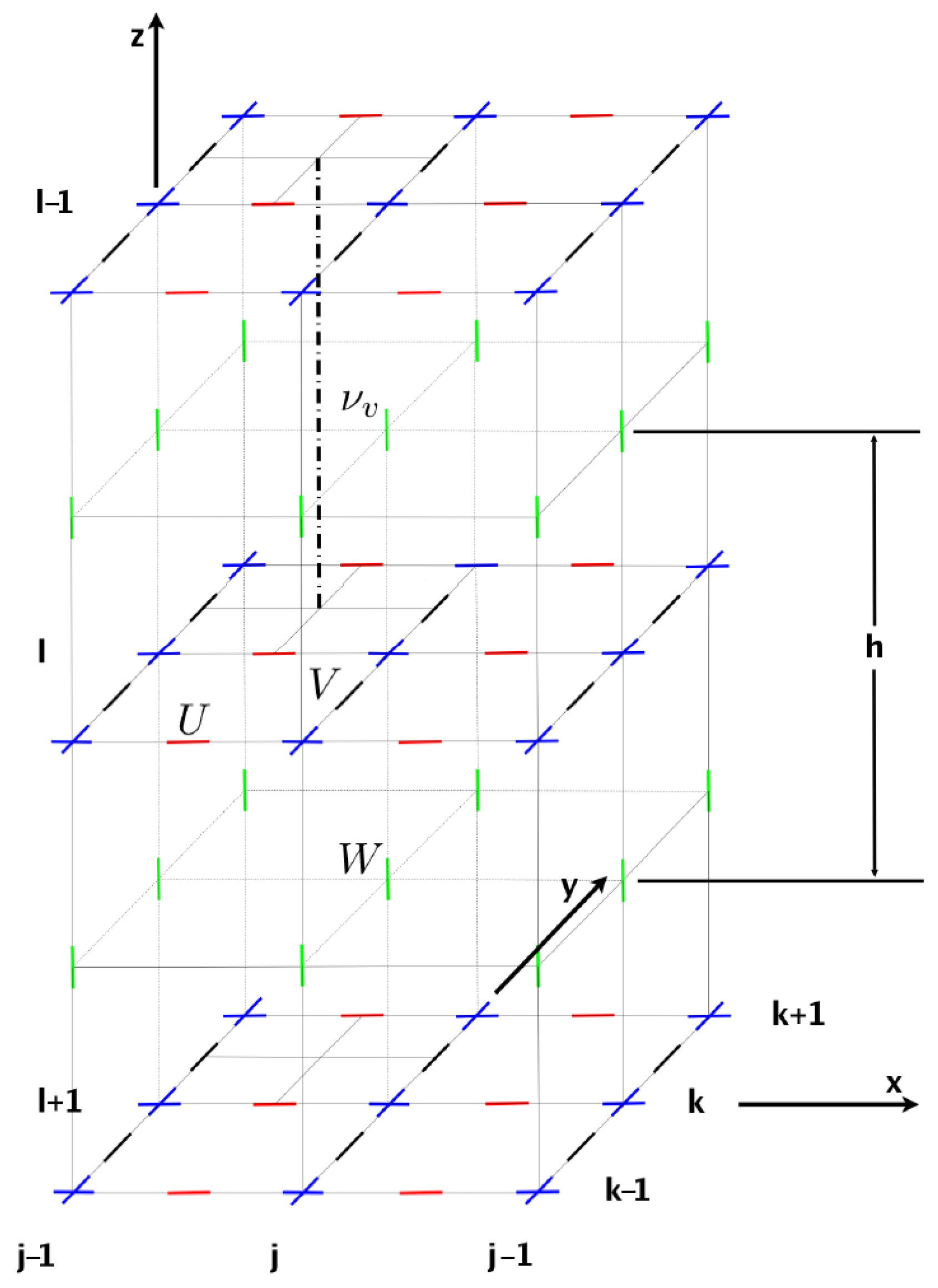
The existence of turbulent velocity fluctuations (Reynolds stresses) introduces additional complexity into the governing equations of motion, rendering the system undetermined. As a result, Reynolds stresses must be modeled. The simplest approach, known as the algebraic (zero-equation) model, expresses turbulent viscosity coefficients as a function of local velocity, while Reynolds stresses are approximated using Boussinesq’s hypothesis:

$$-\ll {\underline{\mathit{u}}}^{\prime }{\underline{\mathit{u}}}^{\prime }\gg =\mathbf{N}·\left[\underline{𝛁}\underline{\mathbf{U}}+{\left(\underline{𝛁}\underline{\mathbf{U}}\right)}^T\right].$$

(11)

Here, the fourth-order tensor $\mathbf{N}=N_{ijkl}$ assigns appropriate turbulent viscosity coefficients ${\nu }_T$ to individual stress terms. These coefficients are not intrinsic properties of the fluid but are instead flow-dependent parameters linked to turbulence characteristics. The precise formulation of ${\nu }_T$ remains a topic of active discussion [36].

In coastal flow modeling, several simplifications are typically applied to turbulence representation, partly due to computational challenges and partly due to limited understanding of turbulence effects on wave-induced currents. It is well established that horizontal turbulent diffusion plays a secondary role, whereas vertical turbulent diffusion is dominant. Consequently, as in quasi-three-dimensional models, the turbulent viscosity coefficient is treated differently in the horizontal (${\nu }_h$) and vertical (${\nu }_v$) directions.

Turbulent viscosity is parameterized using the turbulent velocity scale $\mathcal{U}$ and the mixing length $\mathcal{L}$, as per Prandtl’s hypothesis:

$${\nu }_T\sim \mathcal{U}\mathcal{L}.$$

(12)

However, determining appropriate values for ${\nu }_T$ remains challenging due to limited empirical data on turbulence in the coastal zone [37].

The horizontal turbulent viscosity coefficient ${\nu }_h$ governs velocity smoothing in the cross-shore direction and influences the shift in maximum velocity relative to the wave-breaking location. Among various formulations, this study adopts the expression proposed by Longuet-Higgins [7]:

$${\nu }_h=N_{h}x\sqrt{gD},$$

(13)

where $N_h$ is a dimensionless coefficient (typically in the range 0.0–0.016) and x is the distance from the shore. Here, x serves as the mixing length scale, while the turbulent velocity scale is represented by ${\left(gD\right)}^{1/2}$, corresponding to the maximum orbital velocity at the seabed $u_{bmax}$.

Regarding vertical turbulence, two primary sources are wave breaking and bottom shear stresses. The vertical turbulent viscosity coefficient ${\nu }_v$ controls velocity uniformity along vertical profiles, though observed variations tend to be relatively minor.

While no universal consensus exists on the parameterization of ${\nu }_v$, a widely used zero-equation model by Svendsen and Buhr-Hansen [38] defines it as follows:

$${\nu }_v=N_{v}D\sqrt{gD},$$

(14)

where $N_v$ ranges from $0.01$ to $0.03$. The choice of D as the mixing length scale and wave phase velocity as the turbulent velocity scale is based on experimental studies and applied in real-world conditions.

3.2. Numerical Grid

The numerical solution of the 3D model of wave-generated currents in coastal areas, presented in the previous section, requires the representation of all variables in a discrete form. The space ($x,y,z,t$) is replaced by a grid of evenly spaced points, and each function $f(x,y,z,t)$ is approximated by a discrete multidimensional variable:

$$f_{j,k,l}^m=(x_j,y_k,z_l,t_m),$$

(15)

and each partial derivative is expressed using a finite difference quotient. Naturally, the accuracy increases as the spacing between grid points decreases.

In this study, a staggered numerical grid of the Arakawa C type is employed, as shown in Figure 1 (see, e.g., [39,40]). Staggered grids (also known as decoupled grids), are characterized by the separation of points where different variables are defined, which allows for a straightforward application of central difference schemes and thus enhances the accuracy of the numerical model. The C-type grid is naturally linked to the conservation law scheme, according to which changes in a quantity within a bounded region result from the fluxes of that quantity through the bounding surfaces. The vertical velocity, depth, free surface displacement, and wave parameters are defined at the center of the grid cell, while the velocity components in the x- and y-directions are shifted by half a grid cell width westward and northward, respectively (i.e., they are defined on the cell edges). The velocity component in the vertical direction is shifted by half a grid cell width in the vertical direction. Such grids are commonly used in numerical solutions of hydrodynamic problems.

Staggered grids have become a mainstay of computational fluid dynamics (CFD), supporting applications that range from global ocean general-circulation models to high-resolution simulations of atmospheric acoustics and coastal processes (e.g., [41]). The grid employed here follows this well-established paradigm but is tailored to the specific requirements of wave–current interactions in shallow, breaking-wave environments. This staggering eliminates spurious pressure oscillations and delivers greater numerical stability and accuracy.

The overall finite-difference scheme employed in this study is second-order accurate in space and first-order accurate in time.

The coordinate plane $\mathit{x}=(x,y)$ is placed on the bathymetric map such that the x-axis is perpendicular and the y-axis is parallel to the aligned shoreline. All model data, including depth D and wave parameters (height H, length L, period T, incidence angle $\alpha$), are functions of the position vector $\mathit{x}$. Consequently, all quantities used in the model (scalar, vector, and tensor) are also functions of the position vector. All vectors and tensors are expressed in terms of their components (each of which must be expressed using the variable (15)).

According to the adopted definition of the wave propagation direction $\alpha$ (see Figure 2), the unit vector in the wave propagation direction has the form:

$${\mathit{k}}^0=\left(cos\alpha ,sin\alpha \right).$$

(16)

Similarly, the components of all other vectors are defined, for example:

$$\mathit{q}={\mathit{k}}^0{\left(\rho c\right)}^{-1}E=\left[{\left(\rho c\right)}^{-1}Ecos\alpha ,{\left(\rho c\right)}^{-1}Esin\alpha \right].$$

(17)

In the formulas defining the radiation stress tensor $\mathbf{S}$, which generates flow in the two-dimensional momentum balance equation, the quasi-turbulent stress tensor $\mathit{R}$, which plays a similar role in three-dimensional equations, and the bottom stress tensor ${\tau }_b$, the dyadic (outer) product of the vector ${\mathit{k}}^0$ is used:

$${\mathit{k}}^0{\mathit{k}}^0=∥\begin{array}{cc}{cos}^2\alpha & sin\alpha cos\alpha \\ sin\alpha cos\alpha & {sin}^2\alpha \end{array}∥=∥\begin{array}{cc}{cos}^2\alpha & \frac{1}{2}sin2\alpha \\ \frac{1}{2}sin2\alpha & {sin}^2\alpha \end{array}∥.$$

(18)

Thus, we obtain:

$$\mathbf{S}={\displaystyle \frac{1}{2}}E\left[2\beta {\mathit{k}}^0{\mathit{k}}^0+\left(2\beta -1\right)\mathbf{I}\right]=$$

(19)

$$=E∥\begin{array}{cc}\beta \left(1+{cos}^2\alpha \right)-{\displaystyle \frac{1}{2}}& {\displaystyle \frac{1}{2}}\beta sin2\alpha \\ \\ {\displaystyle \frac{1}{2}}\beta sin2\alpha & \beta \left(1+{sin}^2\alpha \right)-{\displaystyle \frac{1}{2}}\end{array}∥,$$

$$\mathit{R}=\left(2\beta -1\right)D^{-1}E\left[\mathbf{I}-\left(\mathbf{I}-{\mathit{k}}^0{\mathit{k}}^0\right){cosh}^{2}k\left(z+D\right)\right]=$$

$$=K∥\begin{array}{cc}1-\left(1-{cos}^2\alpha \right){cosh}^{2}k\left(z+D\right)& sin\alpha cos\alpha {cosh}^{2}k\left(z+D\right)\\ \\ sin\alpha cos\alpha {cosh}^{2}k\left(z+D\right)& 1-\left(1-{sin}^2\alpha \right){cosh}^{2}k\left(z+D\right)\end{array}∥,$$

where $\beta =c_g/c=\raisebox{1ex}{$1$}\!\left/ \!\raisebox{-1ex}{$2$}\right.\left[1+2kD{\sinh }^{-1}\left(2kD\right)\right]$, $K=\left(2\beta -1\right)D^{-1}E$,

$${\tau }_b={\displaystyle \frac{2}{\pi }}f\rho u_{bmax}\left(\mathbf{I}+{\mathit{k}}^0{\mathit{k}}^0\right)·{\mathit{U}}_b=$$

$$={\displaystyle \frac{2}{\pi }}f\rho u_{bmax}∥\begin{array}{c}{U}_b\left(1+{cos}^2\alpha \right)+V_{b}sin\alpha cos\alpha \\ \\ +U_{b}sin\alpha cos\alpha +V_b\left(1+{sin}^2\alpha \right)\end{array}∥.$$

The solution of the model also requires defining the bottom velocity ${\mathit{U}}_b$, which is a function of the bottom stress tensor. This is done by inverting Equation (10):

$${\mathit{U}}_b={\left({\displaystyle \frac{2}{\pi }}f\rho u_{bmax}\right)}^{-1}{\left(\mathbf{I}+{\mathit{k}}^0{\mathit{k}}^0\right)}^{-1}·{\tau }_b=$$

$$=\pi {\left(4f\rho u_{bmax}\right)}^{-1}∥\begin{array}{cc}1+{sin}^2\alpha & -sin\alpha cos\alpha \\ \\ -sin\alpha cos\alpha & 1+{cos}^2\alpha \end{array}∥·∥\begin{array}{c}{\tau }_{bx}\\ \\ {\tau }_{by}\end{array}∥.$$

(20)

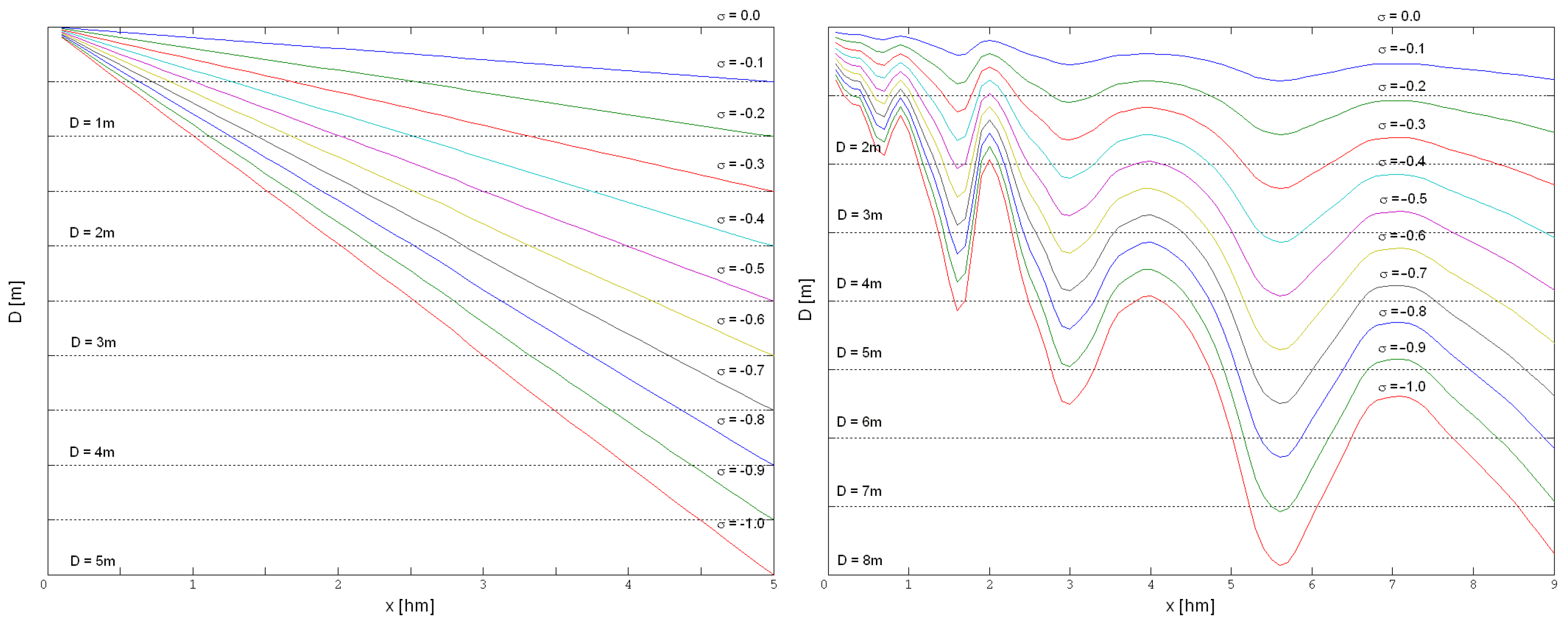
3.3. Sigma Coordinate System

Modeling flows in shallow-water areas necessitates transforming the coordinate system from ($\mathit{x},z$) to ($\mathit{x},\sigma$), where the vertical distance is expressed as a fraction of the total depth. This avoids situations where numerical grid nodes fall outside the study area—i.e., below the seabed, which would occur with a constant water layer thickness in the ($\mathit{x},z$) system (see, e.g., [42]). The “new” coordinate is typically defined as follows:

$$\sigma ={\displaystyle \frac{z-Z(\mathit{x},t)}{D\left(\mathit{x}\right)+Z(\mathit{x},t)}}.$$

(21)

Since the mean free surface displacement Z is a small quantity (relative to other variables in the presented model), a simplified definition of the $\sigma$ coordinate is used in this study:

$$\sigma ={\displaystyle \frac{z}{D\left(\mathit{x}\right)}}.$$

(22)

where D denotes local depth.

The vertical coordinate in the $\sigma$ system varies from 0 at the surface to $-1$ at the seabed. Figure 3 shows the isolines of this coordinate in the ($x,z$) and ($x,\sigma$) systems for a region with a flat sloped bottom and a real bathymetric profile.

As is evident from Equation (22), the vertical coordinate $\sigma$ also depends on the horizontal coordinates. Consequently, derivatives in the ($\mathit{x},z$) system undergo modifications in the ($\mathit{x},\sigma$) system. The partial derivatives of any physical quantity transform as follows:

$${\partial }_z=D^{-1}{\partial }_{\sigma },$$

(23)

$${𝛁=𝛁|}_{\sigma }-D^{-1}\sigma 𝛁D{\partial }_{\sigma },$$

(24)

where ${|}_{\sigma }$ indicates differentiation at $\sigma =const$. Given the previously adopted assumptions (mainly small vertical variability and a gentle bottom slope), the second term on the right-hand side of Equation (24) is omitted in numerical computations. In analytical solutions of the model equations, transformation to the $\sigma$ system primarily serves for better visualization of results.

3.4. Computation Algorithm

All model procedures were coded in the Python 3.11 programming language. The algorithm consists of two blocks: data input and the calculation of quantities directly dependent on them, as well as the simultaneous solution of the two-dimensional and three-dimensional (2D + 3D) model equations.

As mentioned earlier, the model data include wave height, length, period, and approach angle relative to the shore, as well as water depth. Each of these quantities must be stored in a separate text file (ASCII) in columns corresponding to the respective grid rows along the x-axis and rows corresponding to the respective grid rows along the y-axis (see Figure 1). In the specific scenario where all isobaths in the coastal area run parallel to the shoreline, data can be stored in a single-column format. The data from the files are then assigned to the following functions:

$$H\left(\mathit{x}\right),L\left(\mathit{x}\right),T\left(\mathit{x}\right),\alpha \left(\mathit{x}\right),D\left(\mathit{x}\right).$$

Next, all quantities that directly depend on the input data are computed. These include wave energy, coefficient $\beta$, components of wave-induced volumetric transport, the classical radiation stress tensor, and the quasi-turbulent stress tensor:

$$E\left(\mathit{x}\right),\beta \left(\mathit{x}\right),{\nu }_h\left(\mathit{x}\right),{\nu }_v\left(\mathit{x}\right),q_x\left(\mathit{x}\right),q_y\left(\mathit{x}\right),S_{xx}\left(\mathit{x}\right),S_{xy}\left(\mathit{x}\right),S_{yy}\left(\mathit{x}\right),$$

$$R_{xx}(\mathit{x},\sigma ),R_{xy}(\mathit{x},\sigma ),R_{yy}(\mathit{x},\sigma )$$

along with all its further applied integrals. Turbulent viscosity is computed using the modified Formulas (13) and (14):

$${\nu }_h=N_h\left(x\sqrt{gD}+x_2\sqrt{g{D}_2}\right)$$

(25)

$${\nu }_v=N_v\left(D\sqrt{gD}+D_2\sqrt{g{D}_2}\right)$$

(26)

where the index 2 denotes the second grid row parallel to the y-axis (the first corresponds to the shoreline).

The computational block, involving the solution of the two-dimensional model equations, as well as the three-dimensional model equations, begins by initializing the first approximations of bottom friction and the mean free surface displacement:

$${\tau }_{bx}\left(\mathit{x}\right)=0,{\tau }_{by}\left(\mathit{x}\right)=0,Z\left(\mathit{x}\right)=0,\mathrm{for}t=0.$$

(27)

The next step is solving the equations:

$${\partial }_t{Q}_x=-gD{\partial }_{x}Z-{\rho }^{-1}\left({\partial }_x{S}_{xx}+{\partial }_y{S}_{xy}+{\tau }_{bx}\right)+{\left[{\partial }_y{\nu }_h{\partial }_y{Q}_x\right]}_p,$$

(28)

$${\partial }_t{Q}_y=-gD{\partial }_{y}Z-{\rho }^{-1}\left({\partial }_x{S}_{xy}+{\partial }_y{S}_{yy}+{\tau }_{by}\right)+{\left[{\partial }_x{\nu }_h{\partial }_x{Q}_y\right]}_p,$$

(29)

$${\partial }_{t}Z=-\left[{\partial }_x\left(Q_x+q_x\right)+{\partial }_y\left(Q_y+q_y\right)\right],$$

(30)

The bottom friction in subsequent approximations for the 2D model equations is determined according to the formula:

$${\tau }_{bx2D}={\displaystyle \frac{2}{\pi }}f\rho u_{bmax}\left[{\displaystyle \frac{Q_x}{D}}\left(1+{cos}^2\alpha \right)+{\displaystyle \frac{Q_y}{D}}sin\alpha cos\alpha \right],$$

(31)

$${\tau }_{by2D}={\displaystyle \frac{2}{\pi }}f\rho u_{bmax}\left[{\displaystyle \frac{Q_x}{D}}sin\alpha cos\alpha +{\displaystyle \frac{Q_y}{D}}\left(1+{sin}^2\alpha \right)\right].$$

(32)

where $\mathit{Q}=(Q_x;Q_y)$ denotes depth-integrated internal current-generated volumetric transport.

The computations conclude when the maximum difference between ${\tau }_b$ and ${\tau }_{b3}$ is less than 25

Additionally, the following boundary conditions are applied in the 2D + 3D loop:

• At the shoreline:

  $$Q_x+q_x=0,$$

  (33)

  $$Q_y=0,$$

  (34)

  $$U=U_2{Q}_x{D}_2/\left(Q_{x2}D\right),$$

  (35)

  $$V=0;$$

  (36)
• At other boundaries—no gradients in directions perpendicular to these boundaries.

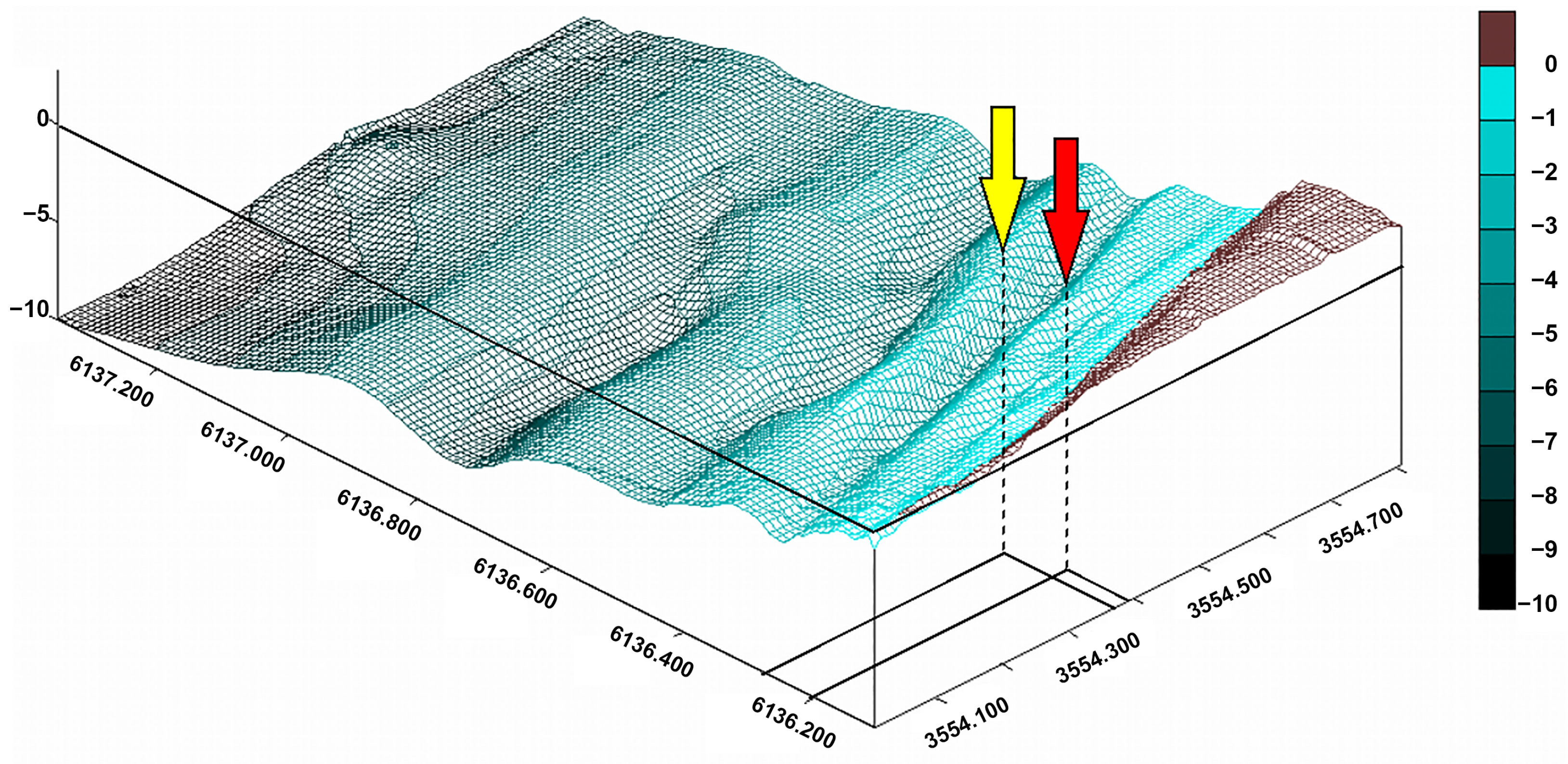
3.5. Input Data

Three sets of bathymetric data were prepared: the first, labeled as I, represents a flat seabed with a constant slope; the second (II) is a multibar profile maintaining alongshore homogeneity; and the third (III) corresponds to the actual seabed topography of the coastal zone in the Lubiatowo region. The depth values corresponding to these datasets are presented in Figure 4 and Figure 5.

The SWAN (Simulating WAves Nearshore) numerical wave model [5] was used for wave modeling in coastal zones I–III. This model describes the frequency-directional wave spectrum and computes approximate wave parameters in coastal areas. The input data for this model include seabed topography, deep-water wave conditions, and wind fields.

The calculations in this study utilized actual deep-water wave conditions recorded by a WR directional wave buoy placed 4600 m offshore at about 20 m depth during the “Lubiatowo 2002” field campaign, and 1850 m offshore at roughly 15 m depth during the “Lubiatowo 2006” campaign. Furthermore, the following data were incorporated:

• Bathymetric data measured during both field campaigns (in addition to depth values, these data also varied in their alongshore extent),
• Homogeneous wind fields measured at the shoreline, including both speed and direction, throughout the field campaigns.

The calculations were conducted in two phases:

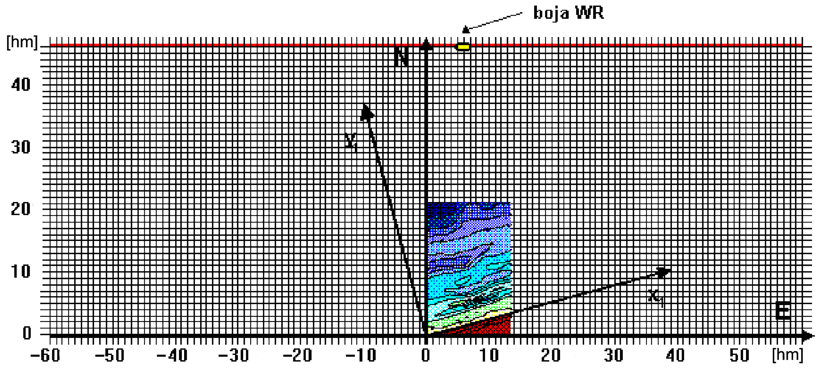
• Using an external grid with a spatial resolution of 100 m × 100 m, spanning a 4600 meter-wide area for the “Lubiatowo 2002” campaign or a 1850 meter-wide area for the “Lubiatowo 2006” campaign, characterized by a flat seabed with a uniform slope,
• Using an internal (smaller) grid with a spatial resolution of 10 m × 10 m, covering the region with detailed seabed topography (cases I–III).

The configuration of both grids for case III, corresponding to real conditions (“Lubiatowo 2002”), is presented in Figure 6. The external grid was defined in a coordinate system where the axes represented geographic directions: east and north (E and N). The seabed was assumed to be flat, sloping so that the offshore boundary depth was 20 m for the “Lubiatowo 2002” data and 15 m for the “Lubiatowo 2006” data. At the offshore boundary, wave conditions were assumed to match those measured by the WR buoy. The values used are presented in

Table 1. Wave parameters in deep water collected during the 2006 Lubiatowo field study.

	H [m]	T [s]	$\alpha$ [°]
A	2.54	6.40	253.13
B	1.75	6.20	233.44
C	2.64	5.33	156.00
D	2.42	5.26	208.41
E	1.80	4.88	202.99
F	1.32	3.96	183.07

.

Seabed topography within the internal grid was defined in the coordinate system of the larger grid. For case III, the computational grid coordinate system was rotated counterclockwise by 17° to align the shoreline with the $x_1$ axis. At the open boundaries of the internal grid, boundary conditions were imposed in the form of a frequency-directional wave spectrum, obtained from calculations on the external grid. All model parameters were selected based on previous studies on SWAN model applications in the coastal zone of the southern Baltic [43].

The simulations were advanced with a constant time step of $\Delta t=2$ s, which satisfies the Courant–Friedrichs–Lewy (CFL) condition (maximum Courant number $\approx 0.55$) for the entire domain. Sensitivity tests with $\Delta t=1$ s and 4 s altered the peak significant-wave-height results by <0.5%, indicating that the chosen time step is sufficiently small for temporal convergence.

4. Results and Discussion

The differential equations of the wave-induced current model in the coastal zone of the sea, presented in [1], along with the proposed solution methods described in the previous section, have a largely prototype-exploratory character due to the inclusion of several novel elements. Consequently, all calculations performed in this study and the results obtained serve primarily as preliminary tests and provide only a very general verification of the model and its solutions. Owing to the model’s limited calibration, difficulties in accurately parameterizing turbulent viscosity—stemming from the insufficient understanding of turbulence in coastal environments—alongside a lack of supporting literature and comparative observational data, the computational outcomes presented in this study should be regarded as indicative.

This section specifically highlights the computational results for two representative bathymetric setups: (I) a coastal area featuring a flat seabed with a constant slope, and (II) a coastal area characterized by a multiple-bar bathymetric profile. For both cases, we assume that all isobaths are parallel to the shoreline, meaning that there are no changes in the y-direction. Additionally, this chapter includes the results of computations for a coastal zone under real conditions (denoted as III). The input data for the model were prepared based on measurements conducted during the measurement expeditions “Lubiatowo 2002” and “Lubiatowo 2006”, carried out at the Marine Coastal Laboratory of the Institute of Hydro-Engineering of the Polish Academy of Sciences in Lubiatowo. Detailed information of the study area is provided in [43,44].

Both surveys employed an identical instrument suite: a Directional Waverider buoy moored, three pressure/velocity tripods, and bottom-mounted ADCPs. The arrays were redeployed along the same cross-shore transect with a positional repeatability better than $\pm 5$ m, and the raw records were processed with a common quality-control and spectral-analysis protocol, yielding a methodologically homogeneous dataset [45,46].

The 2002 record, representative of mild-to-moderate conditions ($H_s=0.3$–$2.6$ m), served mostly for calibration of the bottom-friction coefficient f and the horizontal/vertical eddy viscosities $N_h$ and $N_v$. These parameters were applied to the independent 2006 data, which extended the energy envelope to severe autumn storms ($H_s$ up to $4.7$ m; $H_{max}=7.2$ m). The model performance for 2006 therefore constitutes a reliable test, confirming that the scheme reproduces nearshore hydrodynamics across a wide energy range. Combining the two campaigns thus enhances, rather than compromises, the internal consistency of the study by providing a single-site, rigorously uniform observational continuum embracing both low- and high-energy Baltic conditions.

4.1. Key Notations

• Uppercase letters A–D denote the individual cases of deep-water wave conditions considered in this study.
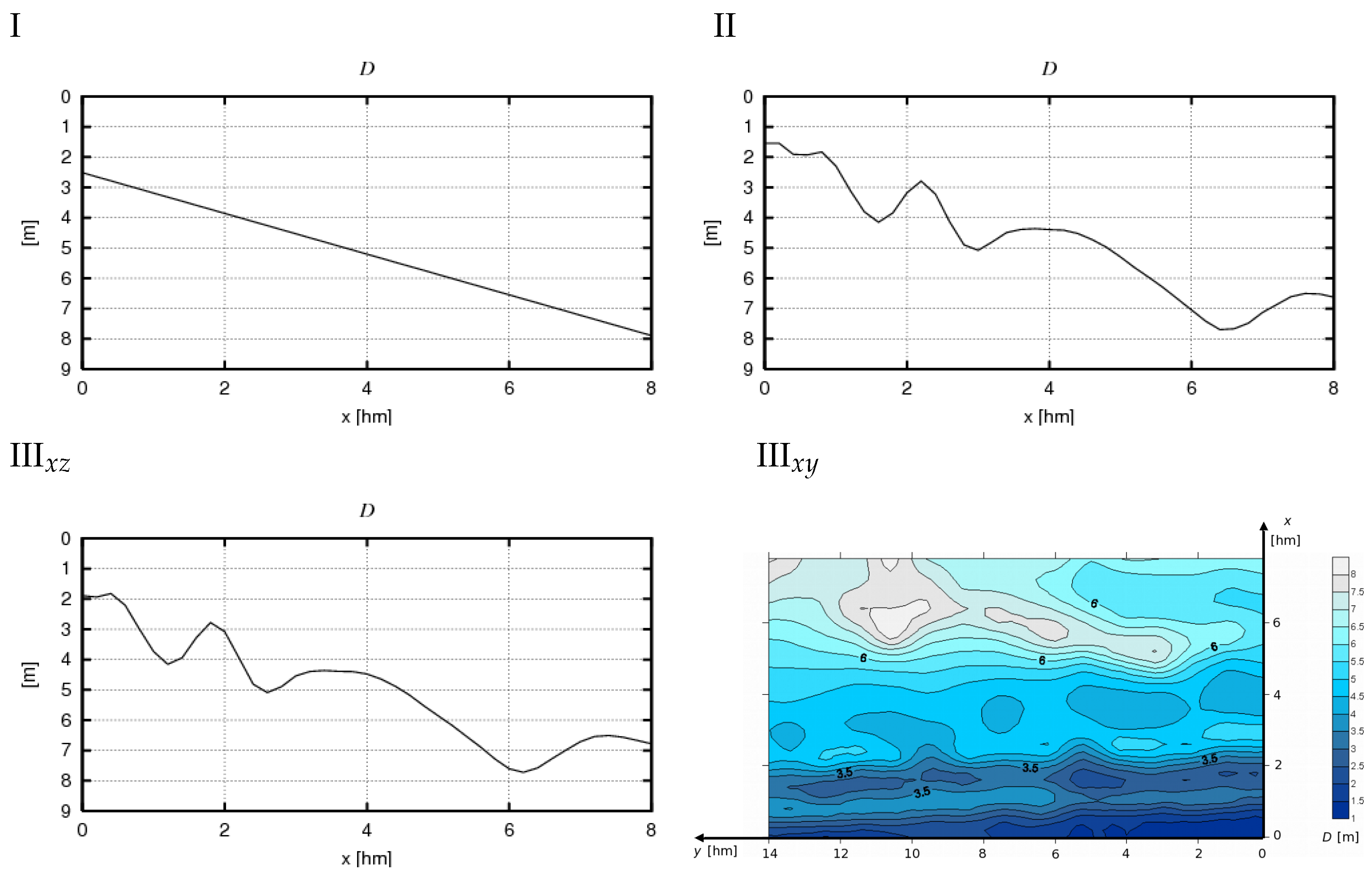
• Roman numerals I–III indicate specific bathymetric cases (ranging from a flat seabed with a constant slope and isobaths parallel to the shoreline to the actual seabed topography in the Lubiatowo region).
• Uppercase calligraphic letters $\mathcal{A}$ and $\mathcal{B}$ distinguish different types of computational procedures used in this study to solve the equations of the three-dimensional model:
  • $\mathcal{A}$—using an analytical solution for general conditions;
  • $\mathcal{B}$—using an analytical solution for specific conditions.
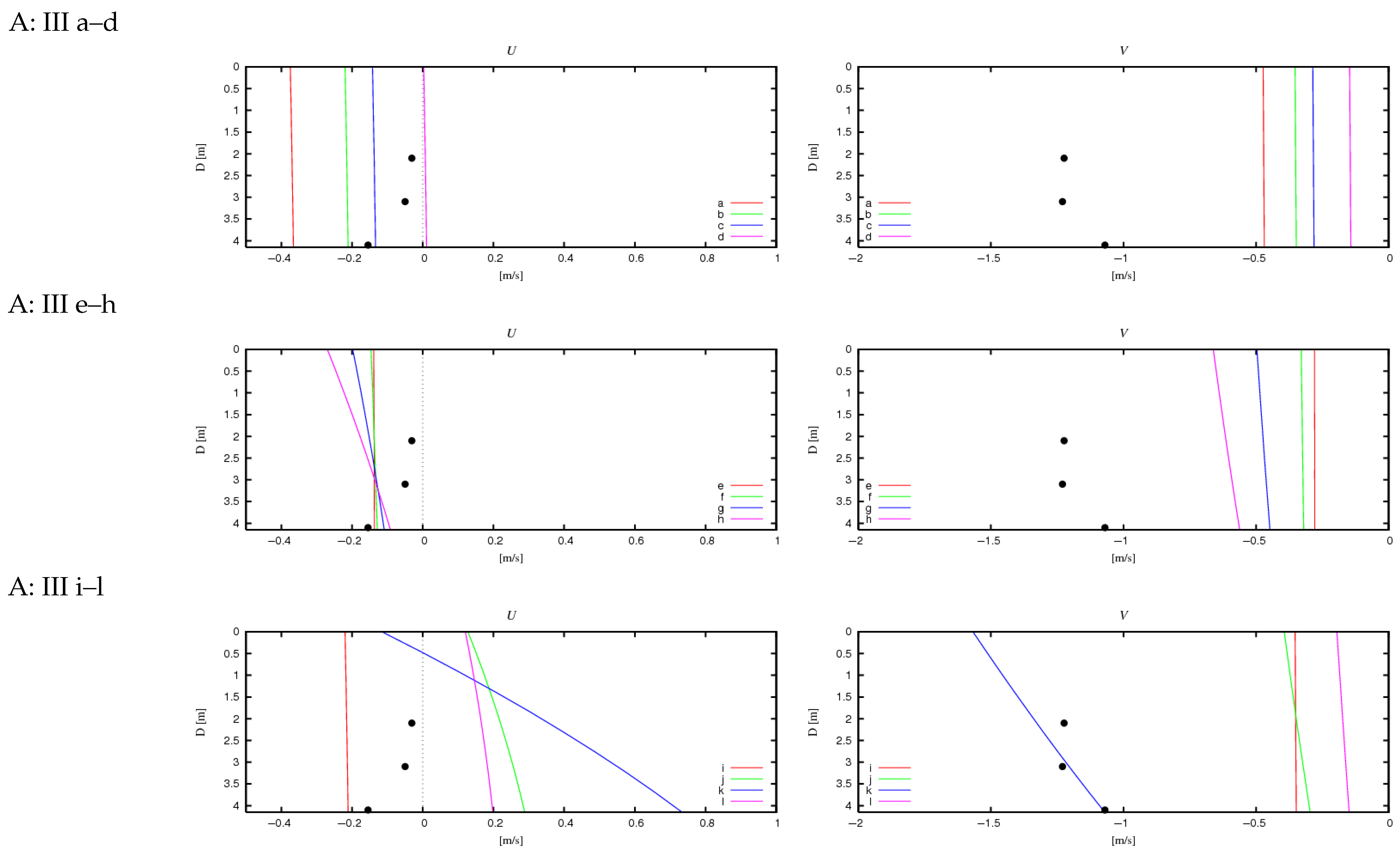
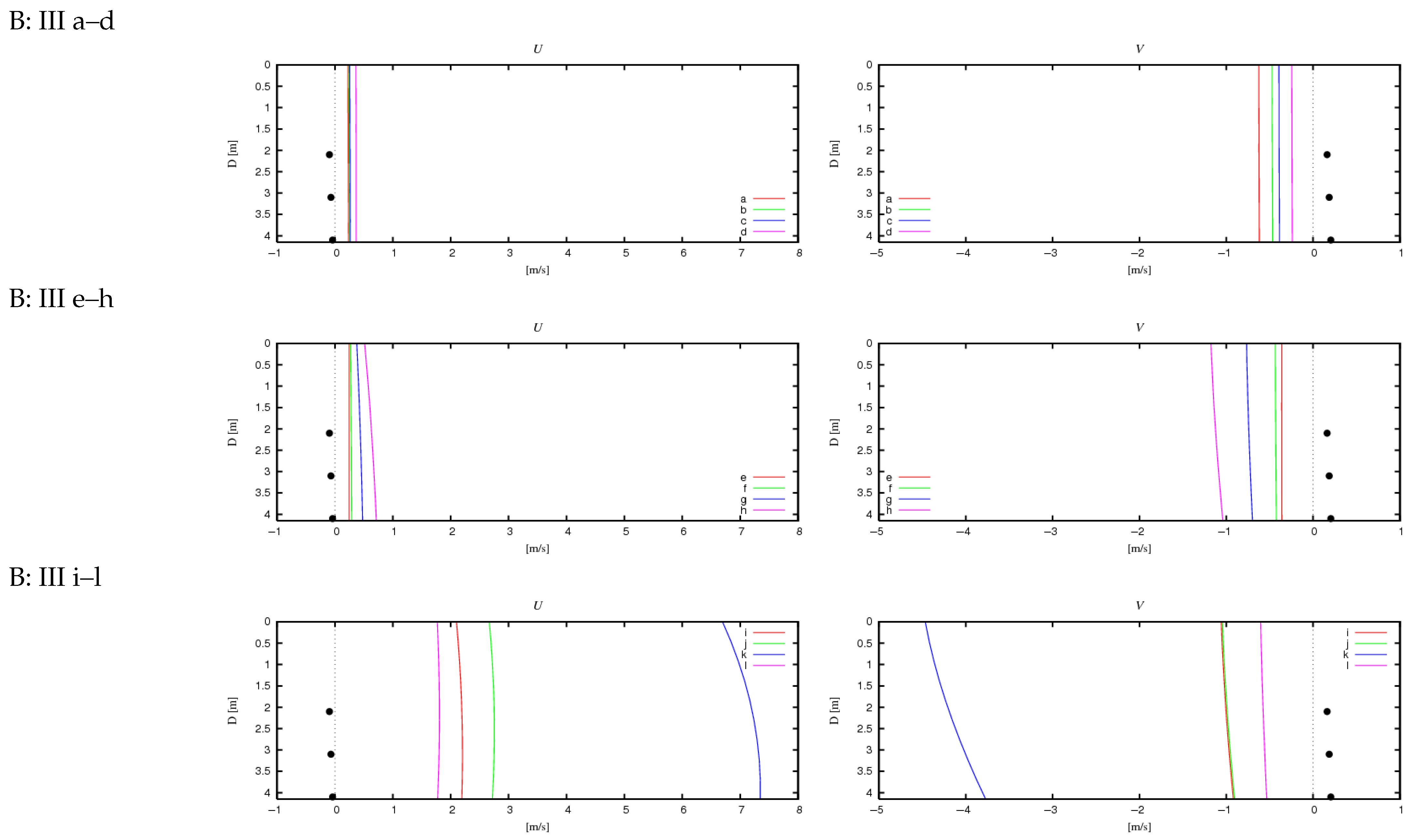
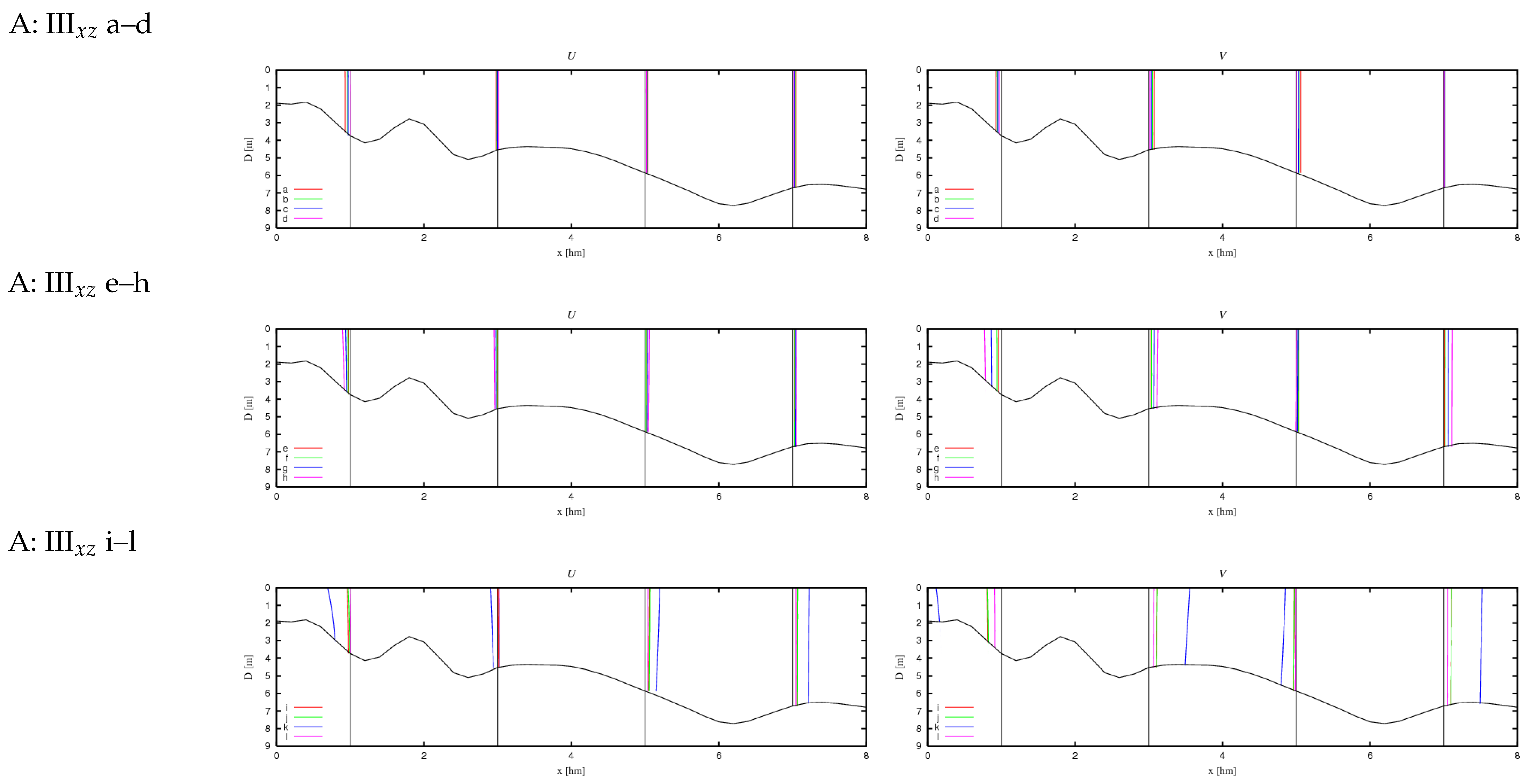
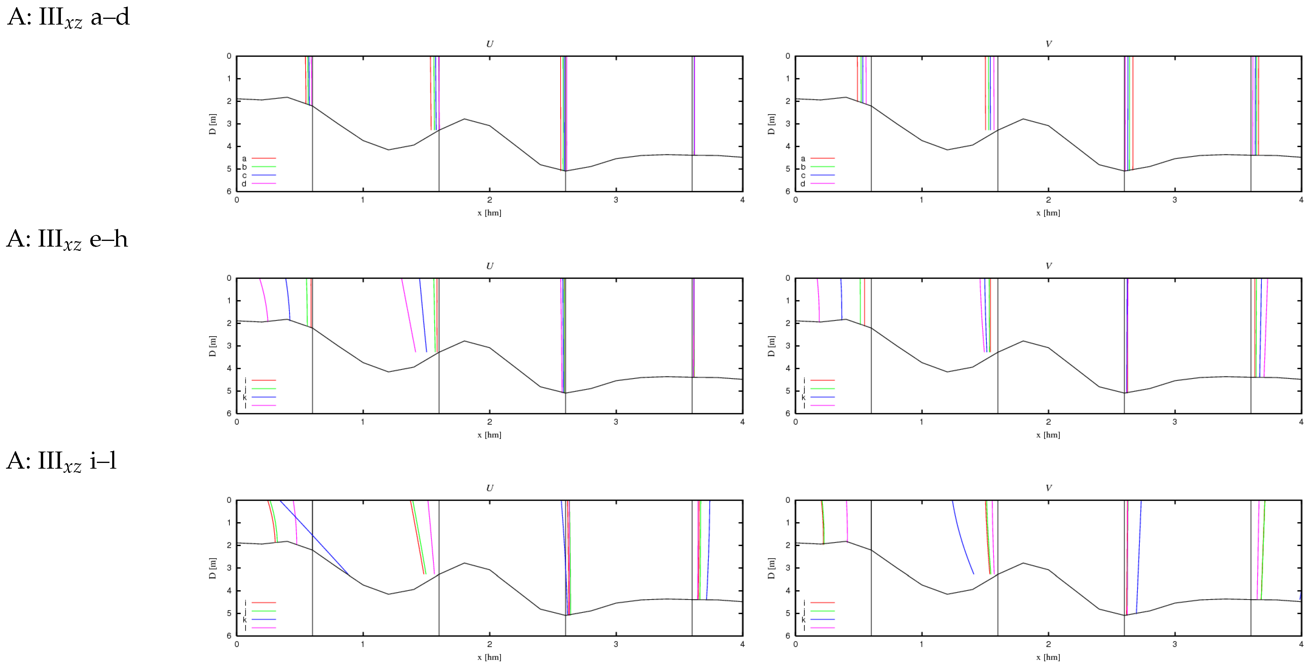
• Lowercase letters a–l denote individual “sets” of coefficients used for computations:

  a:	$f=0.005$	$N_h=0.001$	$N_v=0.01$
  b:	$f=0.0075$	$N_h=0.001$	$N_v=0.01$
  c:	$f=0.01$	$N_h=0.001$	$N_v=0.01$
  d:	$f=0.025$	$N_h=0.001$	$N_v=0.01$
  e:	$f=0.01$	$N_h=0.001$	$N_v=0.05$
  f:	$f=0.01$	$N_h=0.0005$	$N_v=0.005$
  g:	$f=0.01$	$N_h=0.0001$	$N_v=0.001$
  h:	$f=0.01$	$N_h=0.00005$	$N_v=0.0005$
  i:	$f=0.025$	$N_h=0.00005$	$N_v=0.0005$
  j:	$f=0.03$	$N_h=0.0001$	$N_v=0.0005$
  k:	$f=0.02$	$N_h=0.00005$	$N_v=0.0001$
  l:	$f=0.035$	$N_h=0.001$	$N_v=0.001$

4.2. Dependence of Obtained Values on Model Coefficients

In a coastal area featuring a flat seafloor with a consistent slope and uniform conditions along the shore, the calculated average free surface elevation (Z) should align with common variations seen in phenomena like wave set-up and set-down [1]. Therefore, the initial key test of the model involved checking the calculation outcomes for bathymetric case I and related wave conditions (C–F). Furthermore, a spectrum of bottom friction coefficient (f) values was employed in these computations to determine its impact on the resulting values.

The computational findings are presented in Figure 7. The values of the mean free surface elevation allow for the identification of wave set-down and set-up regions, which are located just before the wave breaking line and near the shoreline, respectively. This pattern is consistent across all deep wave conditions. When the bottom friction coefficient is $f=0.01$, the set-down magnitude is close to zero, but it increases as the value of f decreases. These results generally agree with the results of Longuet-Higgins [6], which assume no bottom friction, as well as with findings reported by other researchers (e.g., [47]).

The values of Z for cases C and D are comparable, reflecting the similarity in $H\left(x\right)$ between these cases. The pronounced influence of the wave height function on Z is evident from the results for wave conditions E and F. In these instances, there is both a decrease in surface elevation and a shoreward shift of the minimum values (set-down). The calculations showed that the direction from which the waves approach does not significantly affect Z.

Figure 8 and Figure 9 present a comparison of the computed and measured flow velocity values obtained under real-world conditions during the “Lubiatowo 2006” measurement expedition using an ADCP profiling current meter. The calculations were performed using parameter sets a–l and wave datasets A (Figure 8) and B (Figure 9). The results demonstrate a strong dependence of the computed velocity values on the selection of these coefficients. Notably, certain choices of the parameters f, $N_v$, and $N_h$ can even lead to a reversal in the direction of the cross-shore flow (see Figure 8i–l). This observation underscores the significant influence of parameter selection on the obtained results and highlights the potential for erroneous outcomes if inappropriate values are used.

This finding reinforces the well-known fact that model calibration—an inherently complex task—plays a crucial role in determining the model’s applicability. The velocity values computed for wave dataset A (under certain parameter values) exhibit a reasonable agreement with the measurements; however, different parameter values were required for the alongshore velocity component V and the cross-shore component U. This discrepancy may result from excessive simplifications made in formulating the adopted relationships describing turbulent viscosity in the horizontal and vertical planes. Simultaneously, the computed flow velocity values for wave dataset B differ to some extent from the measured values, with the computed velocity components V and U exhibiting directions opposite to those observed in the measurements—though the measured values are close to zero. It is important to emphasize that naturally occurring currents, unlike the model outputs, exhibit non-stationary behavior. The values presented in Figure 8 and Figure 9 represent measurements averaged over a 30 min period (all ADCP profiles were binned into 30 min averages to suppress high-frequency wave-orbital velocities and instrument noise while retaining wave-driven mean flow).

Additional factors that may contribute to discrepancies between computed and measured values include rip currents, edge waves, infragravity oscillations (surf beats), and potentially certain perturbations associated with turbulence levels, seiches (both surface and internal), and internal waves, which were not accounted for in this study.

Beyond the variability of velocity values within the vertical measurement profile, the analysis also considers the variability of the functions $U\left(z\right)$ and $V\left(z\right)$ as a function of the distance from the shore and the values of the coefficients f, $N_v$, and $N_h$. The results presented in Figure 10 and Figure 11 are intended for illustrative purposes; however, they clearly indicate the significant impact of the parameter values on the computed velocities.

Furthermore, they allow for an assessment of how these coefficients influence flow velocity as a function of distance from the shore (and depth), showing that this influence increases as x decreases, which aligns with expectations. Additionally, the obtained velocity values $U\left(z\right)$ and $V\left(z\right)$ for depths shallower than 2 m raise certain concerns regarding their accuracy. These concerns are directly linked to uncertainties in the wave model results within such shallow regions of the nearshore zone (Zone III).

4.3. Influence of Cross-Shore and Alongshore Bathymetric Variability on the Obtained Results

To assess how variations in bathymetry both across and along the shore affect the calculated values of internal volumetric current transport, bottom friction, free surface elevation, and velocity, the following results are provided for coastal zones I–III and wave datasets A and B.

In general, the following regularities can be observed:

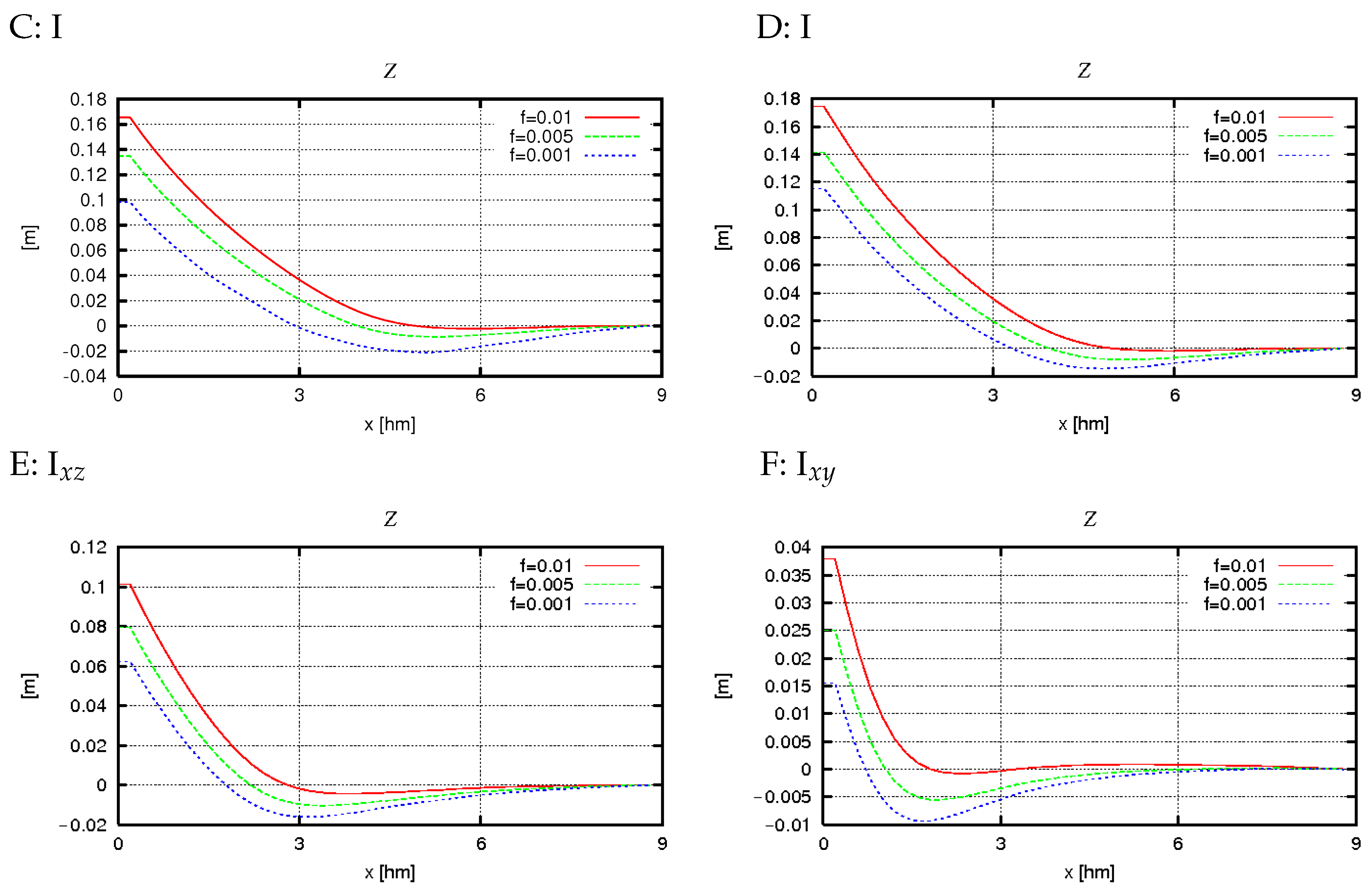
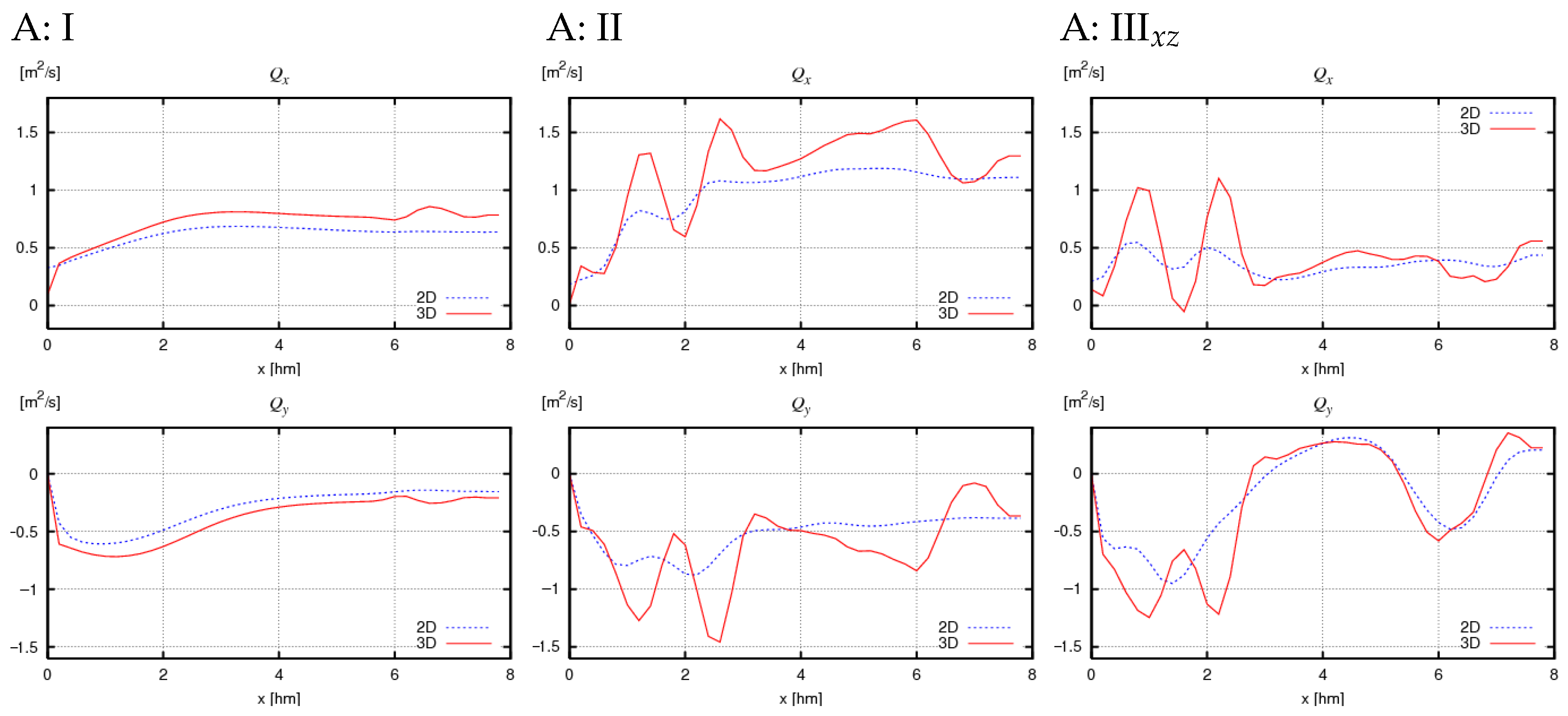
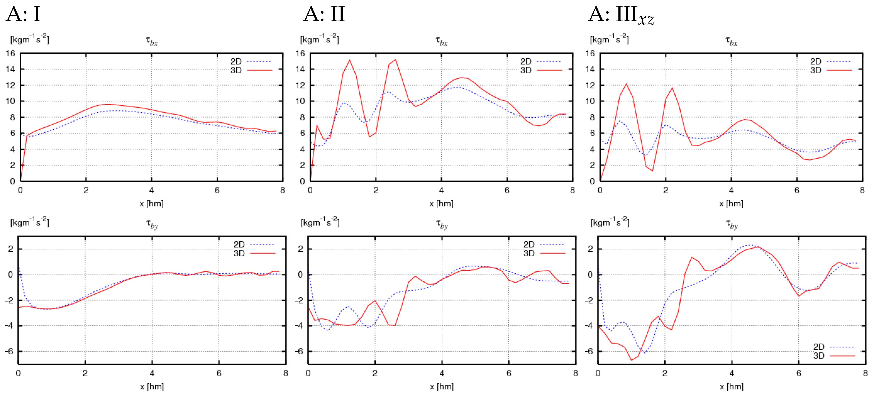
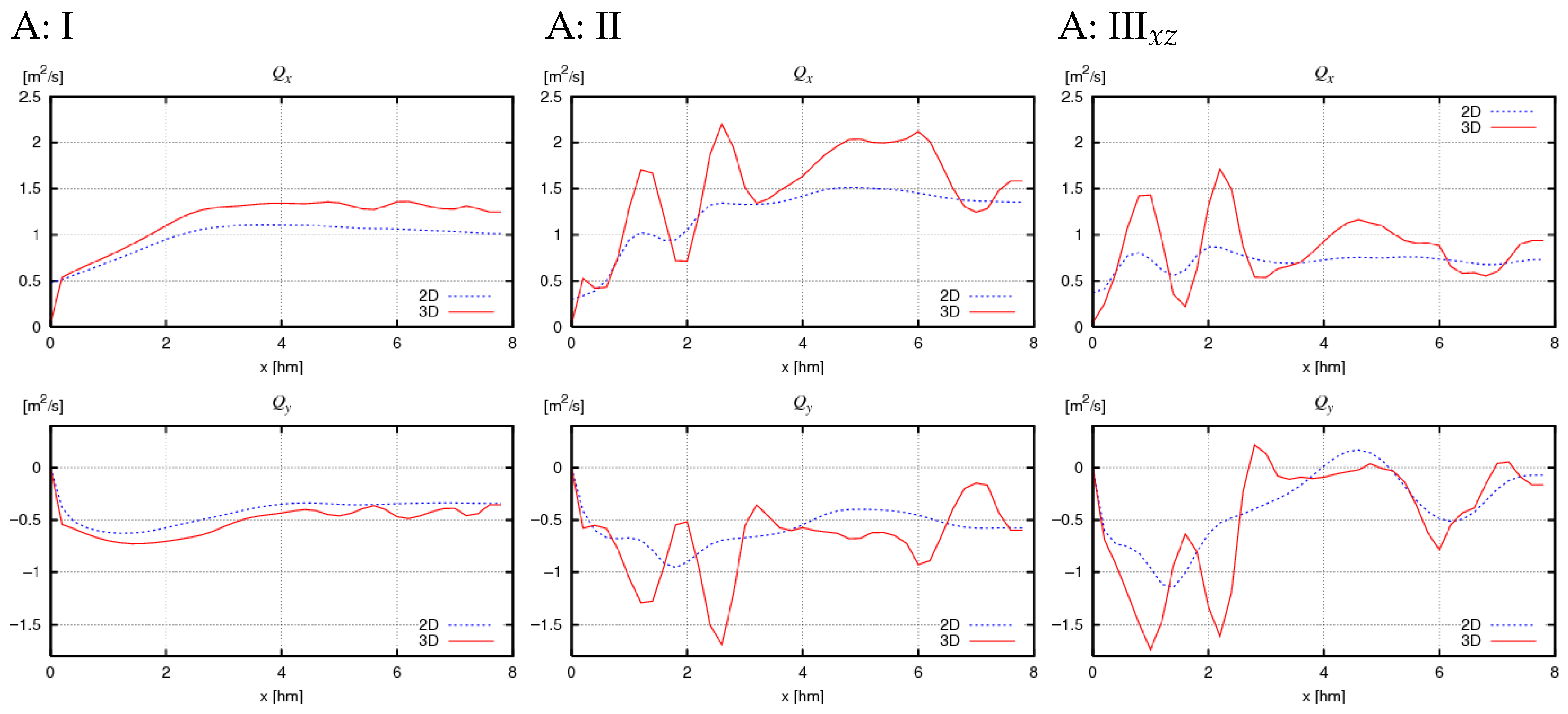
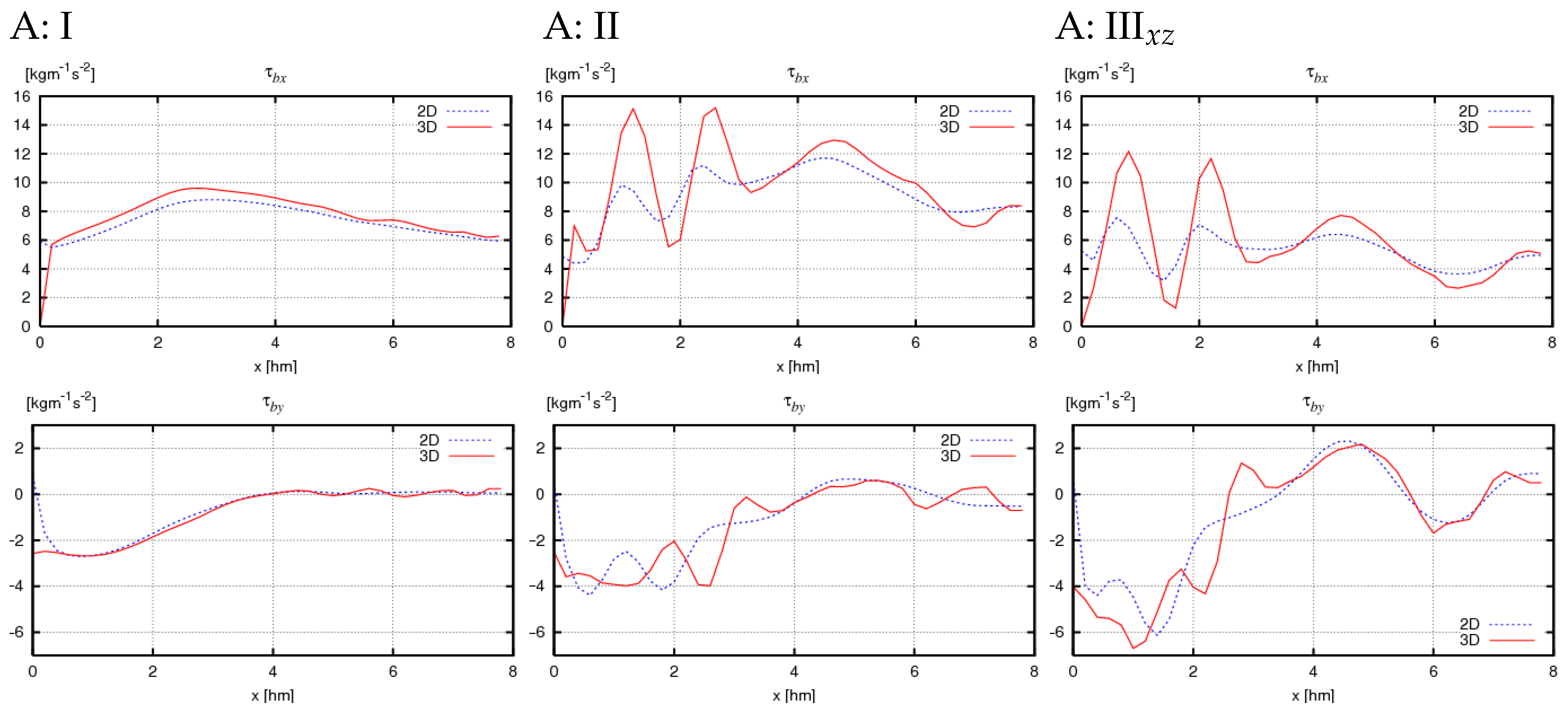
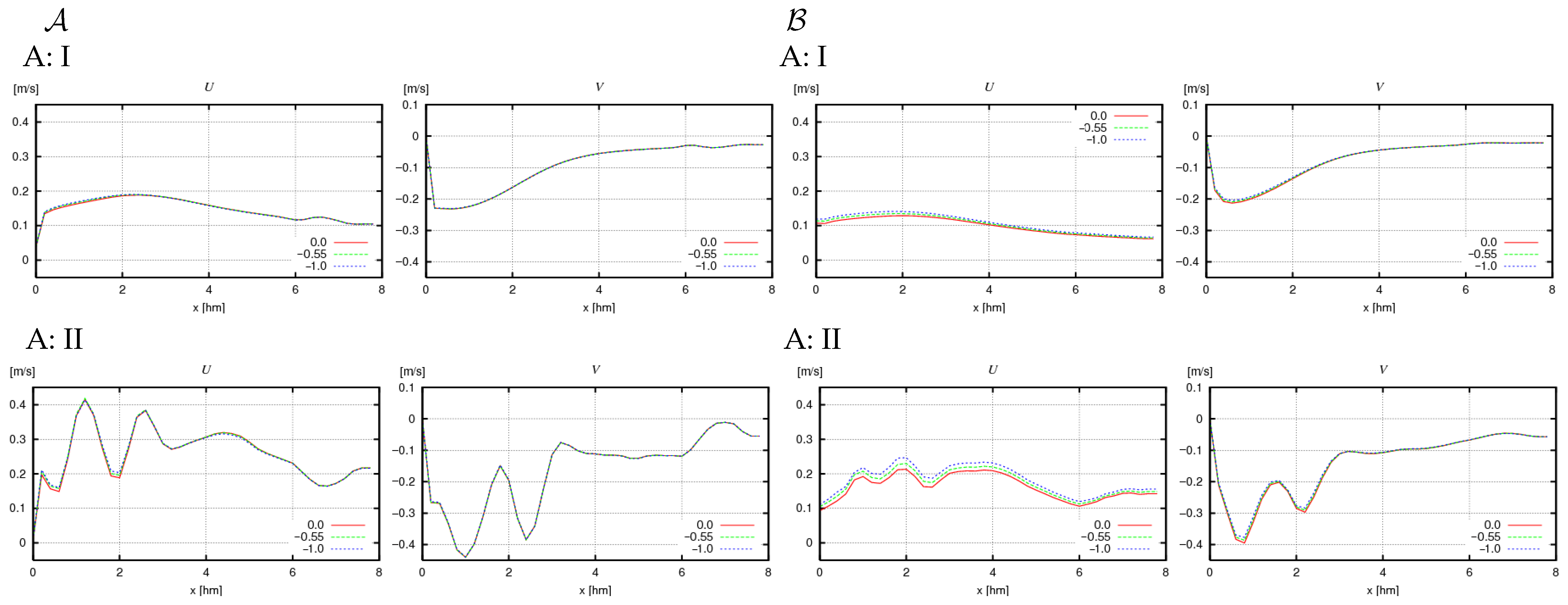
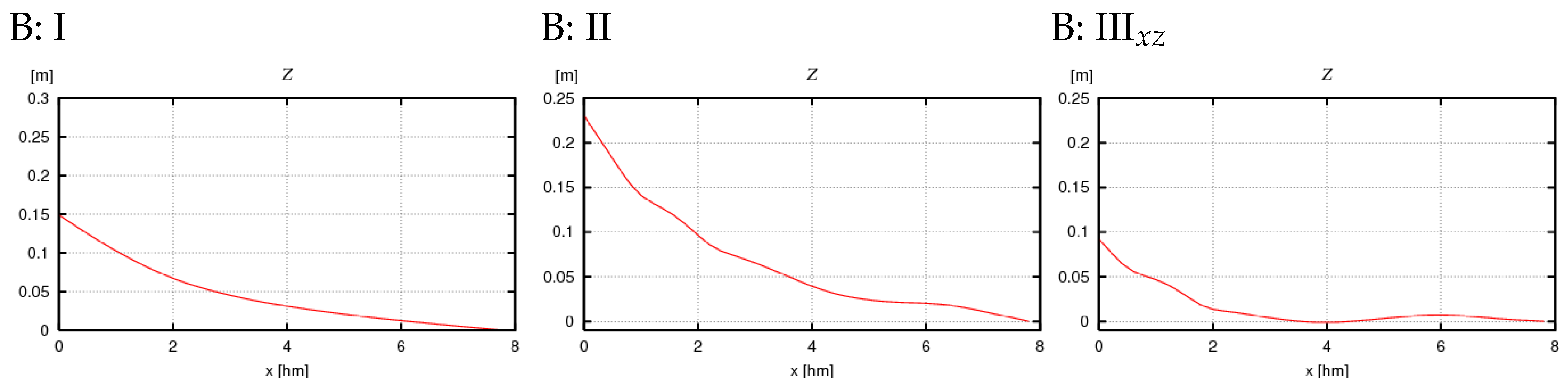
• In the simplest theoretical case (I), the greatest consistency is achieved between the results of the 2D and 3D model equations (values of $\mathit{Q}$ and ${\tau }_b$, see Figure 12, Figure 13, Figure 14 and Figure 15: I). Simultaneously, in this case, as expected, very similar values are obtained for calculations of types $\mathcal{A}$ and $\mathcal{B}$, which utilize analytical solutions for general and specific conditions, respectively (Figure 16 and Figure 17: I).
• Increasing the complexity of the bathymetric profile as a function of distance from the shore, while maintaining alongshore homogeneity (case II), results in increased differences between the 2D and 3D model results and a significant increase in all computed quantities ($\mathit{Q}$, ${\tau }_b$, Z, $\mathit{U}$, Figure 12, Figure 13, Figure 14, Figure 15, Figure 16 and Figure 17: II) relative to case I. Both factors appear to be due to greater variability of wave data in the cross-shore profile while maintaining their variability limits, leading to larger values of derivatives ${\partial }_x$. The discrepancy between the 2D and 3D values for case II arises from the assumptions of both models and may indicate that the 2D model is less sensitive to cross-shore variability, leading to some underestimation of $\mathit{Q}$ and ${\tau }_b$ in coastal zones with real, multi-bar bathymetric profiles and isobaths parallel to the shoreline. The velocity differences obtained for case II from calculations $\mathcal{A}$ and $\mathcal{B}$ (Figure 16 and Figure 17: II) are small (especially in the alongshore component) but noticeably larger than in case I. The results obtained from the analytical solution for specific conditions tend to be lower than those for general conditions.
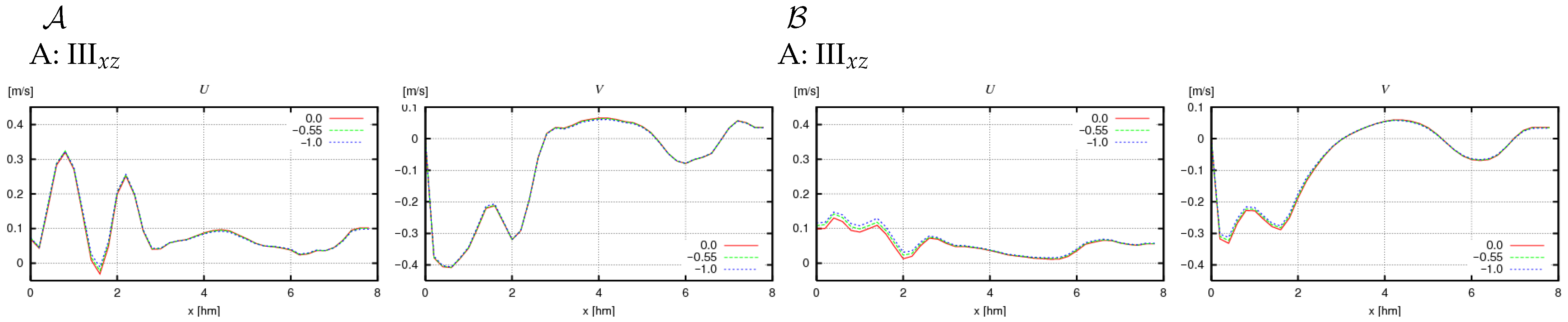
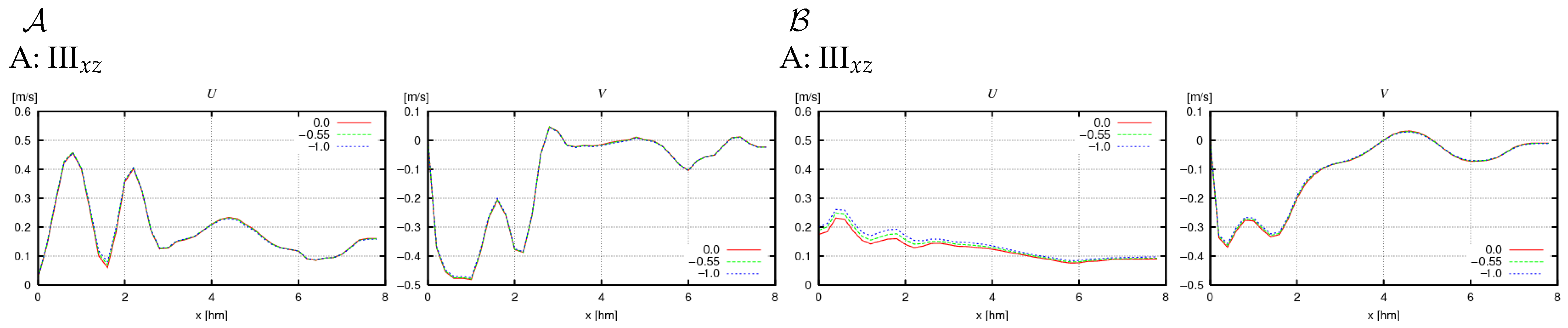
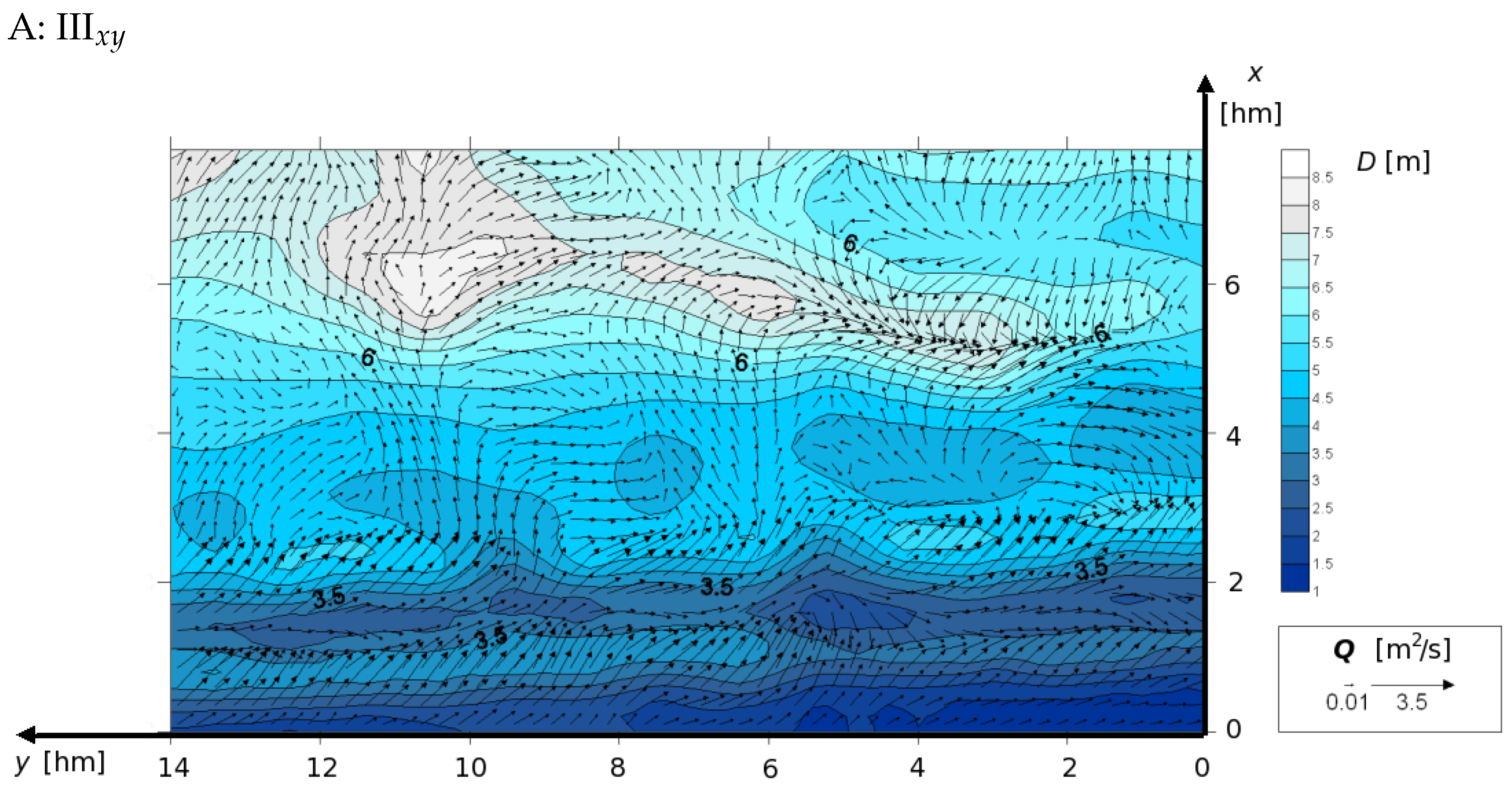
• The presence of nonzero derivatives with respect to the y coordinate in the real case (III) significantly modifies the obtained cross-shore profiles compared to case II. This primarily concerns the change in direction of the alongshore components of volumetric current transport (Figure 12 and Figure 14: III_xz), bottom friction (Figure 13 and Figure 15: III_xz), and velocity (Figure 18 and Figure 19), as well as the values of free surface elevation (Figure 20 and Figure 21: III_xz). The differences between the values obtained using the 2D and 3D model equations are similar to those observed in case II. The velocity results obtained from calculations $\mathcal{A}$ and $\mathcal{B}$ can be used as a preliminary assessment of the influence of the ${\partial }_y$ derivative on the velocity values (since it is not included in $\mathcal{B}$).

The results presented for wave data A and B were obtained for the coefficient values $f=0.01$, $N_v=0.01$, and $N_h=0.001$. Given the resemblance between wave fields A and B, and because the coefficients—which significantly influence the results—were set to the same values, the resulting values for all quantities examined were also similar. The values derived for case B are slightly higher, particularly for the cross-shore components of $\mathit{Q}$, ${\tau }_b$, $\mathit{U}$, and free surface elevation, likely due to a smaller angle of wave approach.

The Z-values obtained (for wave fields A and B) align with both theoretical predictions and field measurements. The absence of the set-down phenomenon for wave data B (Figure 21) and its minimal values for wave data A (Figure 20) across cases I–III can be explained by the assigned bottom friction coefficient, whose influence on Z is discussed in more detail on page 16. Of particular interest is the difference in free surface elevation values between coastal zones II and III. This difference suggests that the derivative with respect to y, often omitted in many Q3D models, significantly impacts the obtained values (not only Z, but also other quantities).

The velocity results (for conditions A and B) indicate that there is minimal variation with depth (Figure 16, Figure 18, Figure 17 and Figure 19). This outcome results from the chosen vertical turbulent viscosity coefficient and corresponds closely with observed velocity profiles in the coastal zone. In coastal zones I and II, velocities U are positive and V are negative, which is due to both the assumed alongshore homogeneity and the wave approach direction ($\alpha >190$°). Additionally, the results obtained for these cases (I and II) from calculations $\mathcal{A}$ and $\mathcal{B}$ do not differ substantially. This implies that the analytical solution can be effectively used in areas where isobaths run parallel to the shoreline under certain conditions. The velocity values obtained for real conditions (III) exhibit high variability—not only in magnitude but also in direction. Due to the lack of sufficient measurement data, it is not yet possible to assess whether the shape of the $\mathit{U}\left(x\right)$ function is accurate. However, given the significant impact of the y-derivative, which is included in the presented model, it appears plausible.

To demonstrate the capabilities of the presented model, two-dimensional fields of internal volumetric current transport are shown for wave data A (Figure 22) and B (Figure 23). These figures indicate that the difference between values obtained for data A and B is much greater than inferred from cross-shore profiles alone. The obtained vector fields exhibit substantial variability in both the cross-shore and alongshore directions. These fields allow the identification of certain circulation zones and even regions where rip currents may occur. However, it appears that the advantages of the presented model compared to Q3D models would be more pronounced in more complex coastal areas, such as around islands or peninsulas.

5. Conclusions

The results obtained from the presented three-dimensional model, specifically the averaged free surface elevation and velocity field distributions, are generally in good agreement with both theoretical values (for particular conditions) and measured data in natural conditions (in the coastal zone of the Coastal Research Laboratory, Institute of Hydro-Engineering of the Polish Academy of Sciences, Lubiatowo). This consistency confirms the model’s applicability. Although these findings represent preliminary results, they appear promising and encourage further exploration of the proposed mathematical modeling approach for coastal zone dynamics. The demonstrated ability of the model to capture essential hydrodynamic processes, including the effects of three-dimensional bathymetric variability and radiation stress formulation, underscores its potential utility for more advanced coastal engineering applications. Future research will aim to refine model resolution and validate results under a broader range of real-world conditions, ensuring its robustness in predictive modeling for coastal management and infrastructure development.

Critical Assumptions and Recommendations for Future Work

While the present model successfully captures three-dimensional wave–current interactions, it relies on several simplifying assumptions whose impacts merit closer scrutiny. In particular:

• Linear wave theory and omission of the surf-zone roller. By using Airy theory and neglecting roller dynamics, non-linear wave breaking effects and short-wave energy fluxes are only crudely represented. Future studies should evaluate the sensitivity of nearshore currents to higher-order wave kinematics and explicit roller models.
• Turbulence closure. The zero-equation eddy-viscosity approach, with constant coefficients $N_h$ and $N_v$, enforces a fixed vertical mixing structure. It will be important to compare against the more advanced two-equation or Reynolds-stress closures, especially under energetic, barred profiles.
• Bottom stress formulation. We employed a linearized tensorial form valid for weak currents. Extensions to fully quadratic, direction-dependent drag laws should be tested in strong flood–ebb and oblique wave conditions.

Addressing these assumptions through targeted field measurements, laboratory experiments, and alternative turbulence and wave-breaking parameterizations will strengthen the model’s predictive capability across diverse coastal settings.

References

1. Gic-Grusza, G. The Three-Dimensional Wave-Induced Current Field: An Analytical Model. Water 2024, 16, 1165. [Google Scholar] [CrossRef]
2. Hill, C.; Marshall, J. Application of a Parallel Navier-Stokes Model to Ocean Circulation in Parallel Computational Fluid Dynamics. In Parallel Computational Fluid Dynamics: Implementations and Results Using Parallel Computers; Elsevier Science B.V.: New York, NY, USA, 1995; pp. 545–552. [Google Scholar]
3. Blumberg, A.F.; Mellor, G.L. A description of a three-dimensional coastal ocean circulation model. In Three Dimensional Coastal Ocean Models 4; Heaps, N., Ed.; American Geophysical Union: Washington, DC, USA, 1987; pp. 1–16. [Google Scholar]
4. Shchepetkin, A.F.; McWilliams, J.C. The Regional Oceanic Modeling System (ROMS): A split-explicit, free-surface, topography-following-coordinate oceanic model. Ocean Model. 2005, 9, 347–404. [Google Scholar] [CrossRef]
5. Booij, N.; Holthuijsen, L.H.; Ris, R.C. A third-generation wave modelfor coastal regions. J. Geophys. Res. 1999, 104, 7649–7666. [Google Scholar] [CrossRef]
6. Longuet-Higgins, M.S. Longshore currents generated by obliquely incident sea waves (1). J. Geophys. Res. 1970, 75, 6778–6789. [Google Scholar] [CrossRef]
7. Longuet-Higgins, M.S. Longshore currents generated by obliquely incident sea waves (2). J. Geophys. Res. 1970, 75, 6790–6801. [Google Scholar] [CrossRef]
8. De Vriend, H.J.; Stive, M.J.F. Quasi-3d modelling of nearshore currents. Coast. Eng. 1987, 11, 565–601. [Google Scholar] [CrossRef]
9. Sánchez-Arcilla, A.; Collado, F.; Lemos, M.; Rivero, F. Another quasi-3d model for surf-zone flows. In Proceedings of the 22nd International Conference on Coastal Engineering, ASCE, Delft, The Netherlands, 2–6 July 1990; pp. 316–329. [Google Scholar]
10. Garcez-Faria, A.F.; Thornton, E.B.; Stanton, T. A quasi-3d model of longshore currents. In Proceedings of the Coastal Dynamics’95—International Conference of Coastal Research in terms of large scale experiments, ASCE, Gdansk, Poland, 4–8 September 1995; pp. 389–400. [Google Scholar]
11. Nobuoka, H.; Mimura, N.; Kato, H. Three-dimensional nearshore currents model based on vertical distribution of radiation stress. In Proceedings of the 26th International Conference on Coastal Engineering, ASCE, Copenhagen, Denmark, 22–26 June 1998; pp. 829–842. [Google Scholar]
12. Mellor, G.L. The three-dimensional current and surface wave equations. J. Phys. Oceanogr. 2003, 33, 1978–1989. [Google Scholar] [CrossRef]
13. Mellor, G.L. Some consequences of the three-dimensional currents and surface wave equations. J. Phys. Oceanogr. 2005, 35, 2291–2298. [Google Scholar] [CrossRef]
14. Mellor, G.L. The depth-dependent current and wave interaction equations: A revision. Phys. Oceanogr. 2008, 38, 2587–2596. [Google Scholar] [CrossRef]
15. Kumar, N.; Voulgaris, G.; Warner, J.C. Implementation and modification of a three-dimensional radiation stress formulation for surf zone and rip-current applications. Coast. Eng. 2011, 58, 1097–1117. [Google Scholar] [CrossRef]
16. Chou, Y.-J.; Holleman, R.C.; Fringer, O.B.; Stacey, M.T.; Monismith, S.G.; Koseff, J.R. Three-dimensional wave-coupled hydrodynamics modeling in South San Francisco Bay. Comput. Geosci. 2015, 85, 10–21. [Google Scholar] [CrossRef]
17. Marin, F.; Vah, M. Cross-Shore Sediment Transport in the Coastal Zone: A Review. Water 2024, 16, 957. [Google Scholar] [CrossRef]
18. Ranasinghe, R.S. Modelling of waves and wave-induced currents in the vicinity of submerged structures under regular waves using nonlinear wave-current models. Ocean Eng. 2022, 247, 110707. [Google Scholar] [CrossRef]
19. Tang, S.; Yang, Y.; Zhu, L. Directing Shallow-Water Waves Using Fixed Varying Bathymetry Designed by Recurrent Neural Networks. Water 2023, 15, 2414. [Google Scholar] [CrossRef]
20. Xia, H.; Xia, Z.; Zhu, L. Vertical variation in radiation stress and wave-induced current. Coast. Eng. 2004, 51, 309–321. [Google Scholar] [CrossRef]
21. Kołodko, J.; Gic-Grusza, G. A note on the vertical distribution of momentum transport in water waves. Oceanol. Hydrobiol. Stud. 2015, 44, 563–568. [Google Scholar] [CrossRef]
22. Mellor, G.L. On theories dealing with the interaction of surface waves and ocean circulation. J. Geophys. Res. Oceans 2016, 121, 4474–4486. [Google Scholar] [CrossRef]
23. Svendsen, I.A.; Putrevu, U. Surf-zone hydrodynamics. In Advances in Coastal and Ocean Engineering; Liu, P.L., Ed.; World Scientific: Singapore, 1996; pp. 1–78. [Google Scholar]
24. Rivero, F.J.; Arcilla, A.S. On the vertical distribution of u ~ w ~ . Coast. Eng. 1995, 25, 137–152. [Google Scholar] [CrossRef]
25. Svendsen, I.A. Wave heights and set-up in a surf zone. Coast. Eng. 1984, 8, 303–329. [Google Scholar] [CrossRef]
26. Svendsen, I.A.; Lorenz, R.S. Velocities in combined undertow and longshore currents. Coast. Eng. 1989, 13, 55–79. [Google Scholar] [CrossRef]
27. Bradford, S.F. Numerical simulation of surf zone dynamics. J. Waterw. Port Coast. Ocean Eng. 2000, 126, 1–13. [Google Scholar] [CrossRef]
28. Marino, M.; Faraci, C.; Jensen, B.; Musumeci, R.E. Turbulent features of nearshore wave–current flow. Ocean Sci. 2024, 20, 1479–1493. [Google Scholar] [CrossRef]
29. Peruzzi, C.; Vettori, D.; Poggi, D.; Blondeaux, P.; Ridolfi, L.; Manes, C. On the influence of collinear surface waves on turbulence in smooth-bed open-channel flows. J. Fluid Mech. 2021, 924, A6. [Google Scholar] [CrossRef]
30. Longuet-Higgins, M.S.; Stewart, R.W. Radiation stress in water waves; a physical discussion with applications. Deep-Sea Res. 1964, 11, 529–562. [Google Scholar]
31. Liu, C.; Clark, A. Analysing the impact of bottom friction on shallow water waves over idealised bottom topographies. Geophys. Astrophys. Fluid Dyn. 2023, 117, 107–129. [Google Scholar] [CrossRef]
32. Jonsson, I.G. Wave boundary layers and friction factors. In Proceedings of the 10th International Conference on Coastal Engineering, ASCE, Tokyo, Japan, 5–8 September 1966; pp. 127–148. [Google Scholar]
33. Whitford, D.J.; Thornton, E.B. Bed shear stress coefficients for longshore currents over a barred profile. Coast. Eng. 1996, 27, 243–262. [Google Scholar] [CrossRef]
34. Kołodko, J. The Tensorial Nature of Bottom Friction in the Coastal Zone of the Sea; Institute of Hydro-Engineering of the Polish Academy of Sciences: Gdańsk, Poland, 1999; internal materials. [Google Scholar]
35. Svendsen, I.A.; Putrevu, U. Nearshore circulation with 3-D profiles. In Proceedings of the 22nd International Conference on Coastal Engineering, ASCE, Delft, The Netherlands, 2–6 July 1990; pp. 241–254. [Google Scholar]
36. Elsner, J.W. Turbulencja przepływów; Państwowe Wydawnictwo Naukowe PWN: Warszawa, Poland, 1987. (In Polish) [Google Scholar]
37. Lozier, M.; Deshpande, R.; Zarei, A.; Lindic, L.; Abu Rowin, W.; Marusic, I. Defining the mean turbulent boundary layer thickness based on streamwise velocity skewness. arXiv 2025, arXiv:2502.00157. [Google Scholar]
38. Svendsen, I.A.; Buhr-Hansen, J. Cros-shore currents in surf zone modelling. Coast. Eng. 1987, 12, 23–42. [Google Scholar] [CrossRef]
39. Middlecoff, J.; Yu, Y.; Govett, M. Performance comparison of the A-grid and C-grid shallow-water models on icosahedral grids. Int. J. High Perform. Comput. Appl. 2022, 37, 197–208. [Google Scholar] [CrossRef]
40. Brodeau, L.; Rampal, P.; Olason, E.; Dansereau, V. Implementation of a brittle sea ice rheology in an Eulerian, finite-difference, C-grid modeling framework: Impact on the simulated deformation of sea ice in the Arctic. Geosci. Model Dev. 2024, 17, 6051–6082. [Google Scholar] [CrossRef]
41. Gilbert, R.P.; Guyenne, P.; Li, J. Simulation of a mixture model for ultrasound propagation through cancellous bone using staggered-grid finite differences. J. Comput. Acoust. 2013, 21, 1250017. [Google Scholar] [CrossRef]
42. Li, Y.; Wang, D.; Wang, B. A New Approach to Implement Sigma Coordinate in a Numerical Model. Commun. Comput. Phys. 2012, 12, 1033–1050. [Google Scholar] [CrossRef]
43. Dudkowska, A.; Boruń, A.; Malicki, J.; Schönhofer, J.; Gic-Grusza, G. Rip currents in the non-tidal surf zone withsandbars: Numerical analysis versus field measurements. Oceanologia 2020, 62, 291–308. [Google Scholar] [CrossRef]
44. Halicki, A.; Dudkowska, A.; Gic-Grusza, G. Short-term wave forecasting for offshore wind energy in the Baltic Sea. Ocean Eng. 2025, 315, 119700. [Google Scholar] [CrossRef]
45. Ostrowski, R.; Pruszak, Z.; Różyński, G.; Szmytkiewicz, M.; Pham Van Ninh, P.; Do Ngoc Quynh, D.; Nguyen Thi Viet Lien, N. Coastal Processes at Selected Shore Segments of South Baltic Sea and Gulf of Tonkin (South China Sea). Arch. Hydro-Eng. Environ. 2009, 56, 3–28. [Google Scholar]
46. Ostrowski, R.; Pruszak, Z.; Skaja, M.; Szmytkiewicz, M.; Trifonova, E.; Keremedchiev, S. Hydrodynamics and lithodynamics of dissipative and reflective shores in view of field investigations. Arch. Hydro-Eng. Environ. 2010, 57, 219–241. [Google Scholar]
47. Mendes, S. A continuous non-ergodic theory for the wave set-up. Eur. J. Mech. B Fluids 2024, 106, 78–88. [Google Scholar] [CrossRef]
Figure 1. Numerical grid of Arakawa C type in space. h—vertical grid step, j—grid row index along the x-axis, k—grid column index along the y-axis, l—layer index.
Water 17 01336 g001
Figure 2. Illustrative representation of the wave incidence angle ( α ).
Water 17 01336 g002
Figure 3. Bottom profile of sloped plane bottom (on the left) and real coastal zone (on the right) resolved by z coordinate (dash line) and by σ coordinate (coloured line).
Water 17 01336 g003
Figure 4. Input data for the model: water depth. (I)—flat-bottom, with constant slope, (II)—multibar profile with isobaths parallel to the shoreline, (III)—realistic bottom topography, specifically: (IIIxz—central) profile of the analyzed area, (IIIxy)—the entire computational area.
Water 17 01336 g004
Figure 5. Bottom topography of Lubiatowo with the layout of current meters during the “Lubiatowo 2002” field campaign.
Water 17 01336 g005
Figure 6. Computational grids in the SWAN model defined for case III.
Water 17 01336 g006
Figure 7. The mean free surface elevation Z derived from calculations A for wave conditions (CF) and bathymetric profile I. These calculations were conducted using various values of the bottom friction coefficient f.
Water 17 01336 g007
Figure 8. Comparison of measured (during the “Lubiatowo 2006” field campaign) current velocities (black dots) with velocity profiles obtained from calculations A for wave parameters A and different values of coefficients f, N v , and N h (Uleft, Vright).
Water 17 01336 g008
Figure 9. Comparison of measured (during “Lubiatowo 2006” field campaign) current velocities (black dots) with the velocity profiles obtained from calculations A for wave parameters B and different values of coefficients f, N v and N h (Uleft, Vright).
Water 17 01336 g009
Figure 10. Cross-shore variability of velocity profiles obtained from calculations A for wave parameters A and different values of coefficients f, N v and N h .
Water 17 01336 g010
Figure 11. Cross-shore variability of velocity profiles U (left) and V (right) obtained from calculations A for wave parameters A and different values of coefficients f, N v and N h (surf zone).
Water 17 01336 g011
Figure 12. Internal mean volume transport Q x (top) and Q y (bottom) obtained from calculations A for wave parameters A and bathymetric data (I)–(III).
Water 17 01336 g012
Figure 13. Bottom friction τ b x (top) and τ b y (bottom) obtained from calculations A for wave parameters A and bathymetric data (I)–(III).
Water 17 01336 g013
Figure 14. Internal mean volume transport Q x (top) and Q y (bottom) obtained from calculations A for wave parameters B and bathymetric data (I)–(III).
Water 17 01336 g014
Figure 15. Bottom friction τ b x (top) and τ b y (bottom) obtained from calculations A for wave parameters B and bathymetric data (I)–(III).
Water 17 01336 g015
Figure 16. Current velocity U and V for different values of σ , obtained from calculations ( A ) (left) and ( B ) (right), corresponding to the wave parameters A and the bathymetric data (I)–(II).
Water 17 01336 g016
Figure 17. Current velocity U and V for different values of σ , obtained from calculations ( A ) (left) and ( B ) (right), corresponding to the wave parameters B and the bathymetric data (I)–(II).
Water 17 01336 g017
Figure 18. Current velocity U and V for different values of σ , obtained from calculations ( A ) (left) and ( B ) (right), corresponding to the wave parameters A and the bathymetric (III).
Water 17 01336 g018
Figure 19. Current velocity U and V for different values of σ , obtained from calculations A (left) and B (right), corresponding to the wave parameters B and the bathymetric data (III).
Water 17 01336 g019
Figure 20. The mean free surface elevation Z derived from calculations ( A ) for wave conditions A and bathymetric data (I)–(III).
Water 17 01336 g020
Figure 21. Mean free surface elevation Z obtained from calculations ( A ) for wave parameters B and bathymetric data (I)–(III).
Water 17 01336 g021
Figure 22. Internal mean volume transport Q obtained from calculations ( A ) for wave parameters A and bathymetric data (III).
Water 17 01336 g022
Figure 23. Internal mean volume transport Q obtained from calculations ( A ) for wave parameters B and bathymetric data (III).
Water 17 01336 g023