On the Origin of Sediment Ripples

Abstract

As soon as a granular sediment has been set in motion by the currents of droppable fluids or by wind, sand waves form as smaller ripples or larger dunes. The relevance of this phenomenon lies in the roughness effect against the currents and the influence on sediment loads. Likewise, their physical understanding helps us to estimate past flow conditions by means of fossilized sand waves, as well as those on distant planets with proven ripples and dunes, such as Mars and Titan. In the literature, diagrams exist based on observations for the conditions under which the various forms of sand waves develop. However, the cause of their formation is unclear. Various theories have been discussed regarding the further development of ripples once they have formed, but none of them explains the fundamental mechanism that generates the very first ripples. These occur simultaneously over a large area and almost instantly, with a fairly even distance from crest to crest. This contribution presents a solution for how this is possible based on hydrodynamic instability.

1. Introduction

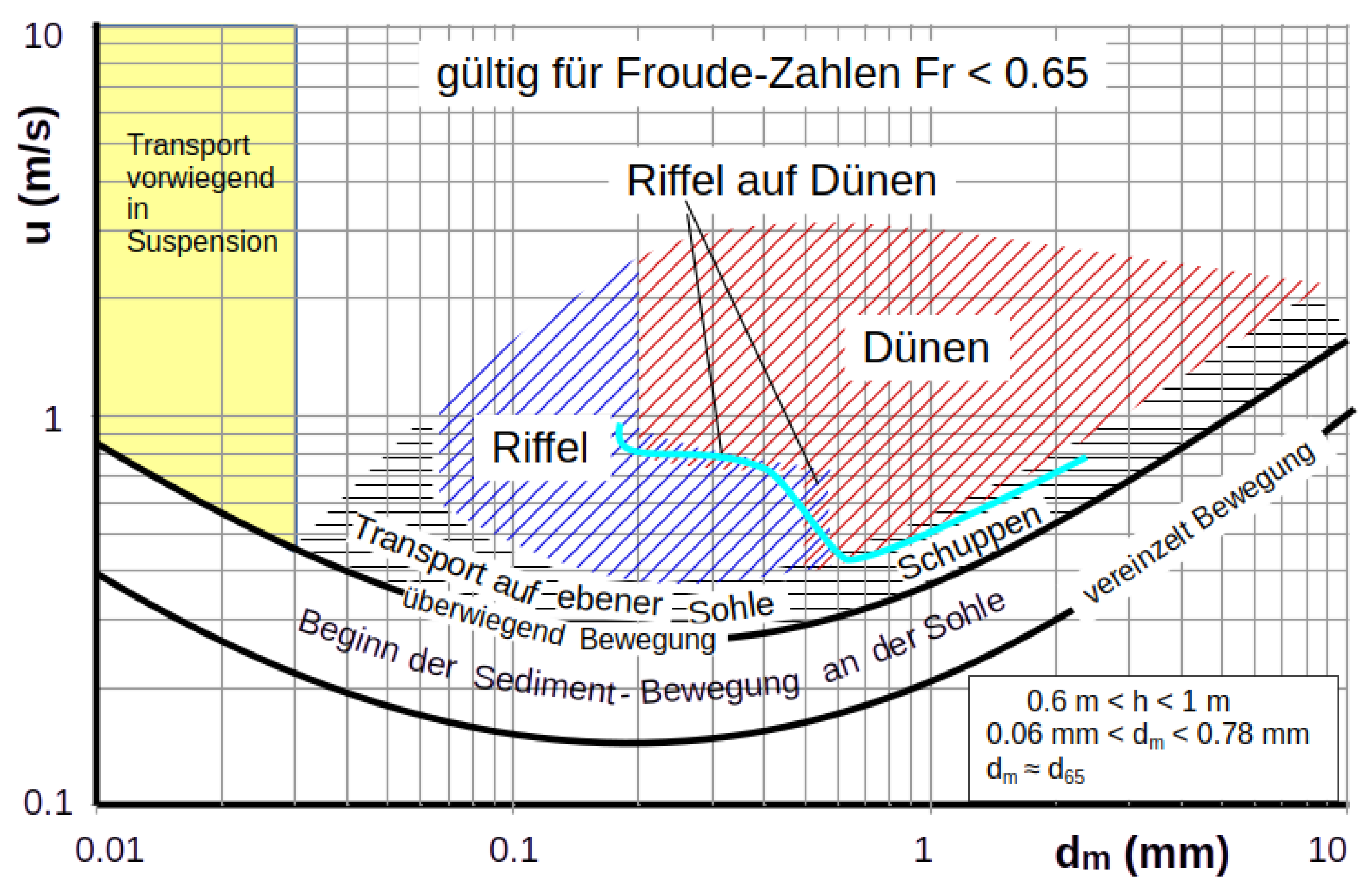
On Earth and other planets, sand waves in the form of ripples and dunes are observed in granular sediments. While dunes can grow to considerable heights (H) and lengths (L), which obviously depend on the available flow depth (h), the size of fully grown ripples is not observed to be influenced by the water depth (as long as $h⪆3H$), but by the grain size (d). On Earth, ripples form in sandy sediments with grain sizes of about $0.06<d\left(\mathrm{mm}\right)<0.6$. They can reach fully developed dimensions of a few centimeters in height and a few decimeters in length. For sand grains $d⪅0.2$ mm, only ripples form, while for $d⪆0.2$ mm, ripples transform into dunes when the flow velocity exceeds a critical value. This critical value is about 2.5 times the velocity at which the sediment movement begins. On Earth, in sand with a diameter of $d⪆0.6$ mm, only dunes form. These can grow under water to heights of about 1/3 of the water depth and, under the influence of wind, can reach heights of more than 100 m. There is thus a clear physical difference between ripples and dunes.

The majority of publications on sand waves deal with their final size and the estimation of the conditions under which ripples or dunes migrate (see, e.g., the diagrams of Chabert and Chauvin 1963 [1], Bonnefille/Pernecker 1963 [2], Vollmers and Giese [2], extended form Wieprecht [3], Zanke 1976/1982 [4,5], Flemming 1988/2019/2022 [6,7,8], Southard and Boguchwal 1990 [9], v.d. Berg and v. Gelder 1993 [10], Baas 1999 [11], Kleinhans 2005 [12], Lamb, Grotzinger, Southard and Tosca 2012 [13], Naqshband and Hulscher 2014 [14] Lapotre, Lamb and McElroy 2017 [15]). These diagrams are essentially based on observations of the sand–water system on Earth. As an example, the dimensioned phase diagram from Zanke 1976/82 [4,5]) is shown here with Figure 1.

The cause behind why ripples occur is unable to be determined from these diagrams, and there is comparatively little literature on this question. In this paper, a theory for the origin of ripples is presented, and is verified using the results of the extensive laboratory experiments conducted by Hardtke 1979 [16] and Venditti et al. 2005 [17].

2. Observations on How Ripples Arise

Hardtke 1979 [16] conducted experiments on the emergence of ripples with sand of $d=0.15$ mm at various flow velocities. He carried out experiments on ripple formation at the Institute for Hydromechanics at the University of Karlsruhe in a closed rectangular laboratory channel of approx. 7 m in length and 0.745 m in width. The channel was operated in a circuit using pumps. The actual test section of 2.1 m at the end of the channel length should thus be free of secondary currents and be fully developed, as Hardtke states. Furthermore, small depth to width ratios (depths of 5 cm and 10 cm) were intended to ensure that the flow had a two-dimensional character. A sand of $d=0.15$ mm is used. In the experiments, both fairly two-dimensional embryonic ripples and those with zigzag crests arise from the first moment of visibility. The latter are referred to by Hardtke as “nose formations”. In the former case, this points to the two-dimensional Tollmien–Schlichting waves (TS) as the trigger, while in the latter case, the $\Lambda$ vortices that follow the TS waves come into question as the cause.

Venditti, Church, and Bennet 2005 [17]) conducted their experiments at the National Sedimentation Laboratory, United States Department of Agriculture, Oxford, Mississippi. They used a tilting recirculating flume with a length of 15.2 m, a width of 1 m, and a depth of 0.30 m, which recirculates both sediment and water. The authors investigate the emergence of ripples in a sand bed with a grain size of $d=0.5$ mm. The authors describe rows of “chevrons” from which the first ripples form. These chevrons obviously correspond to Hardtke’s “nose formations”.

Both authors report that the first ripples or their zigzag precursors arise during the acceleration phase of the flow.

Hardtke starts his experiments by first setting a flow state just below the beginning of the sediment movement. Then, the flow rate is increased as quickly as possible to the setpoint value of the respective experiment. The start of the experiment is thus defined by the moment the sediment movement begins. In the final state of his Experiment IV, for example, $u_m=0.348$ m/s, $u^{★}=0.0188$ m/s, $\nu =1.08$${\mathrm{m}}^2$/s and ${\tau }^{★}=0.145$. Here, $u_m$ is the mean flow velocity, $u^{★}$ denotes the shear velocity, $\nu$ the kinematic viscosity, and

$${\tau }^{★}=\tau /\left(({\rho }_s-\rho )gd\right)=u^{★2}/\left({\rho }^{\prime }gd\right)$$

(1)

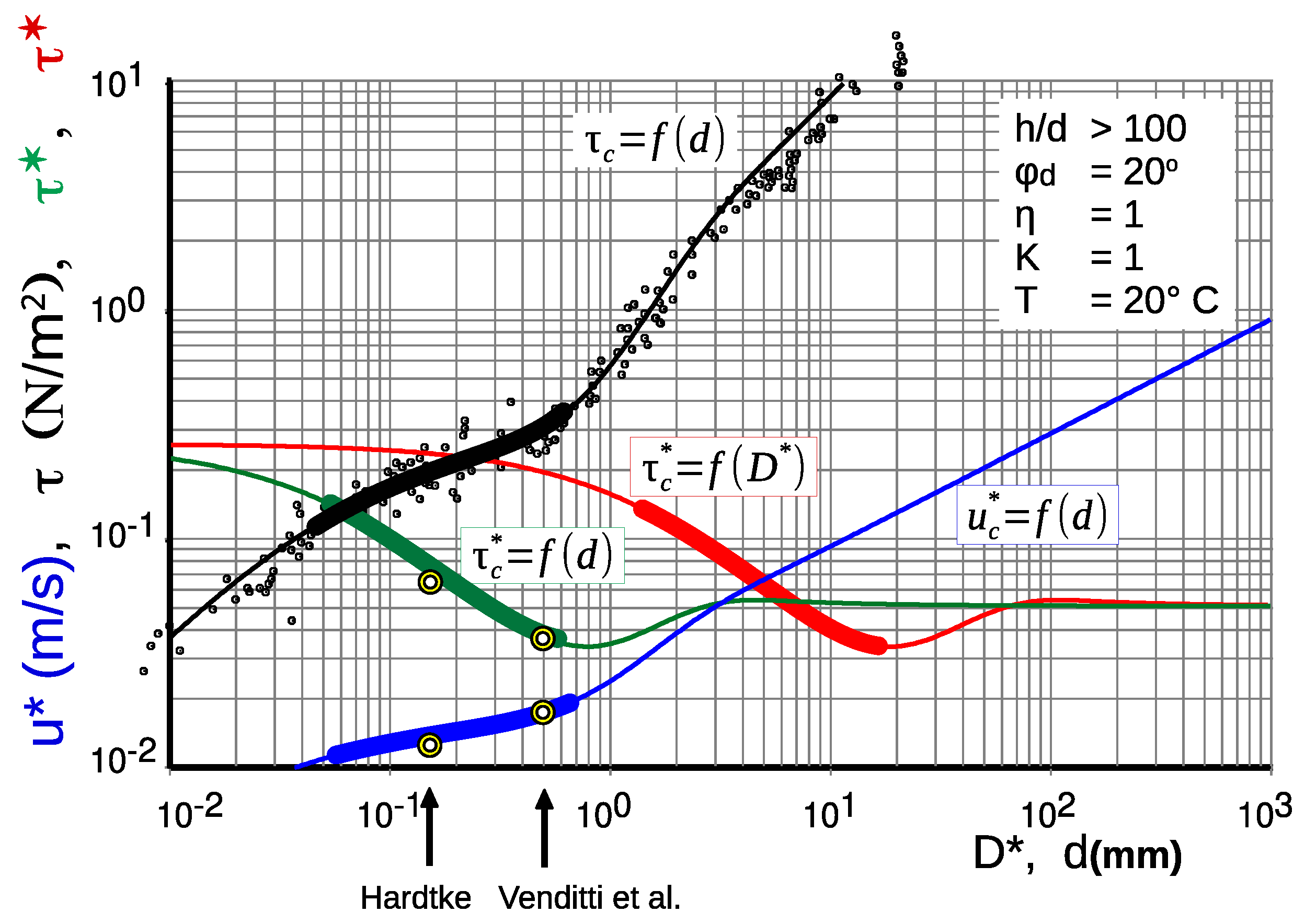
The critical shear stress (i.e., the Shields-curve) can be determined by

$$\begin{array}{|c|}\hline {\tau }_c^{★}=\zeta tan{\phi }_d·K·\eta \\ \hline\end{array}$$

(2)

with

$$\zeta ={\displaystyle \frac{0.714}{1+0.65D^{★}}}+0.14\left(1-EXP(-0.004D^{★1.5})\right).$$

(3)

and

$$D^{★}={\left({\displaystyle \frac{{\rho }^{\prime }g}{{\nu }^2}}\right)}^{1/3}d.$$

(4)

Here, g is the acceleration due to gravity, ${\rho }_s,\rho$ are the densities of sediment and fluid, with the relative density ${\rho }^{\prime }=({\rho }_s-\rho )/\rho )$. K takes into account a cohesiveness (cohesion is assumed not to be present here, i.e., $K=1$) and $\eta$ takes into account a slope effect (a flat bed with $\eta =1$ is assumed here). Furthermore, ${\phi }_d$ is the dynamic angle of the internal friction of the moved sediment, here set to 20 to ${22}^{°}$. The critical shear stress computed in this way corresponds to the Shields curve corrected according to newer measurement data in the fine-grain range. The critical values for the beginning of movement resulting from this calculation are shown in Figure 2. For the purposes of the questions discussed here, this easy-to-solve formulation is fully sufficient. A more in-depth solution for the critical shear stress can be found in e.g., Zanke 2002 [18].

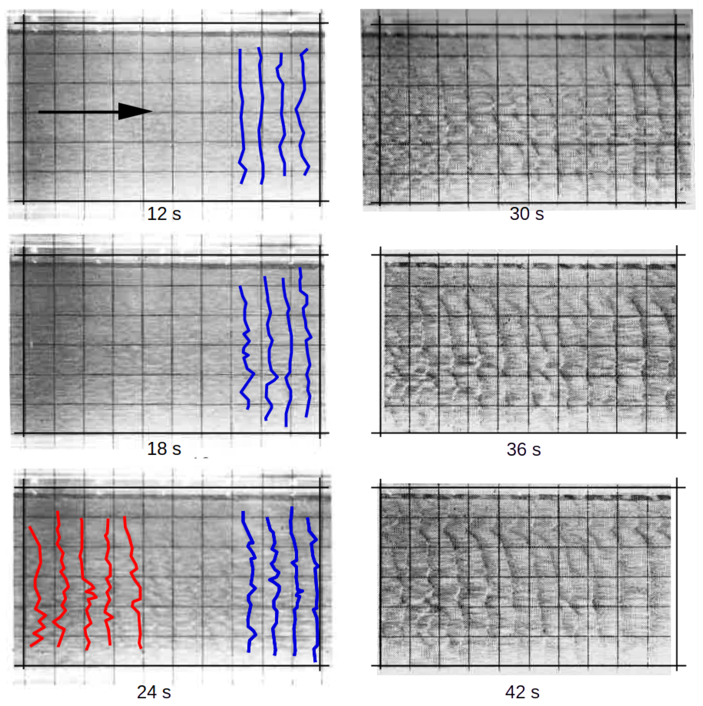
In Hardtke’s Experiment IV, the first ripple crests can be seen in his photos after just 6 s, i.e., soon after the flow starts to accelerate. After 12 s, they have recognizably migrated a little further in the direction of flow (Figure 3; blue positions of the approximate course of the crest).

These initial ripples occurred at the downstream end of the photo section, and were about $L_i=0.035$ m long. After 24 s, initially only vaguely recognizable due to the images not being particularly sharp, further ripple crests with a spacing of $L_i\approx 0.05$ m occurred at the upper end of the photo section (shown in red). At 30 s after the start of the experiment, the first ripples, $L\approx 0.035$ m long, run out of the observation section, and are dominated by the ripples that appeared a little later, with $L\approx 0.05$ m.

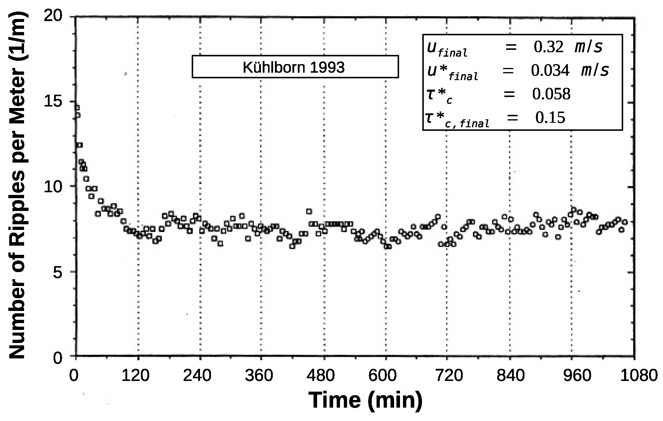
Further results on the length of initial ripples $L_i$ are provided by the evaluations of Kühlborn 1993 [27]. Kühlborn carries out laboratory tests on final ripple dimensions with sand of $d=0.16$ mm, from which the lengths in the state of origin can also be taken. Figure 4 shows the initial number of ripples per meter at around 15. That is, in this experiment, the initial length $L_i\approx 0.06\dots 0.07$ m. Kühlborn gives the mean value of his entire experiments as $L_i\approx 0.075$ m.

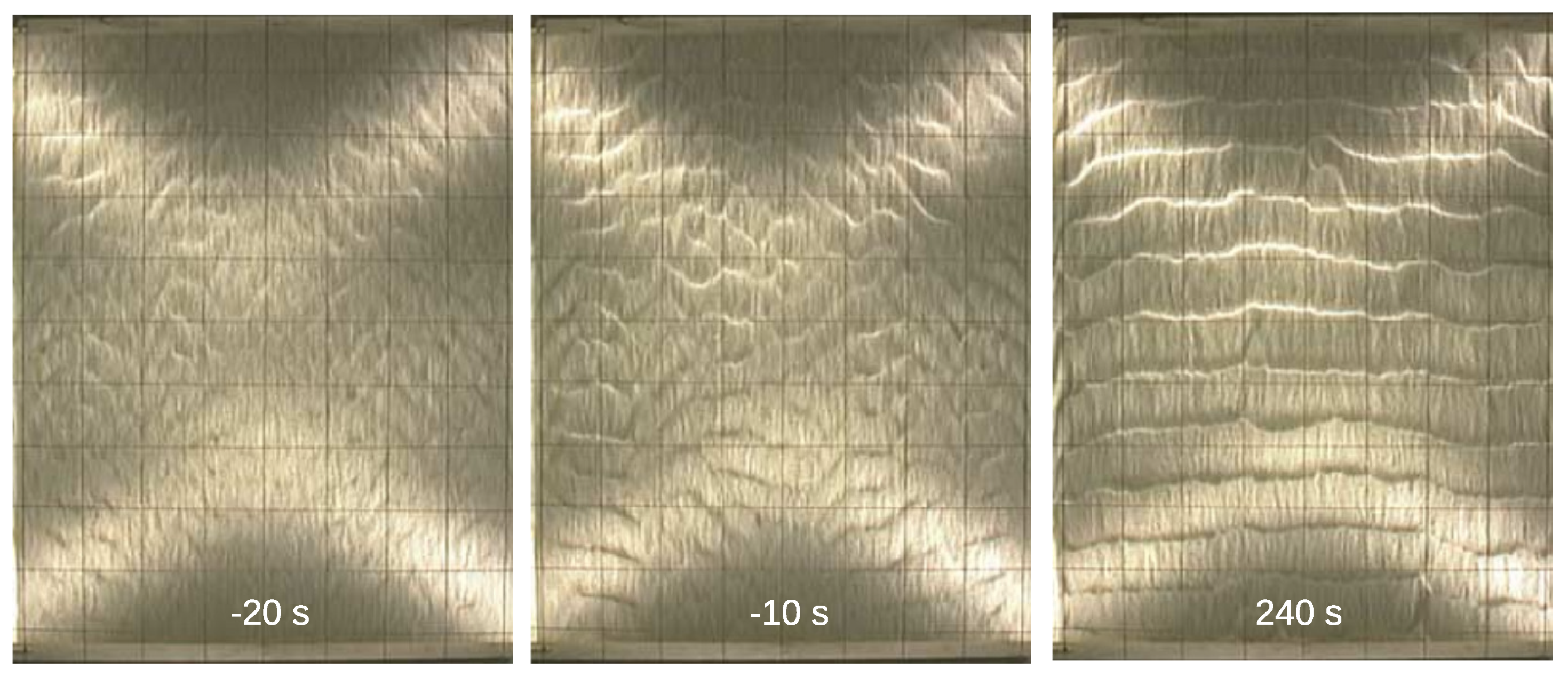
In the experiments by Venditti, Church, and Bennet 2005 [17], with sand of $d=0.5$ mm, the first ripples appear on the previously flat sediment bed even before the intended final flow velocity of the experiment is reached. For their experiment A with the highest flow velocity of $u_m=0.5$ m/s, the ripples already emerge during the ramp-up of the flow, as in Hardtke 1979. Figure 5 shows the initial stage. At −60 s, the bed is still flat, so that the duration until the ripple appears is $t_i<40$. Crests that are largely parallel, as seen in Figure 3 after 42 s, can be seen here after about 240 s.

Table 1. Dominant initial lengths according to laboratory tests with quartz sand in water ( ${\rho }^{\prime }$ = 1.65) and the observed development times $t_i$. Critical shear stresses according to the authors. $u_{c,i}^{★}=1.4u_c^{★}$ is the critical shear stress velocity for the formation of a ripple (see Section 5).

	d	${\mathit{u}}_{\mathit{m}}$	$\mathit{\nu }·{10}^6$	${\mathit{\tau }}_{\mathit{c}}^{\mathit{★}}$	${\mathit{\tau }}_{\mathbf{ci}}^{\mathit{★}}$	${\mathit{u}}_{\mathbf{ci}}^{\mathit{★}}$	${\mathit{L}}_{\mathit{i}}$	${\mathit{L}}_{\mathit{i}}{\mathit{u}}_{\mathit{c},\mathit{i}}^{\mathit{★}}/\mathit{\nu }$	${\mathit{t}}_{\mathit{i}}$
	mm	m/s	m2/s	-	-	m/s	cm	-	s
Hardtke	$0.15$	0.348	$1.08$	$0.065$	$0.13$	0.0176	$3.5$	570	6–12
Hardtke	$0.15$	0.348	$1.08$	$0.065$	$0.13$	0.0176	5	815	15
Kühlborn *	$0.16$	0.321	$1.03$	$0.058$	$0.116$	0.0173	7–8	1260	n.a.
Venditti et al.	$0.5$	0.501	1 **	$0.037$	$0.074$	0.024	$8.5$	1970	<40

Note: * Kühlborn primarily examines the final ripple size. However, one can also extract initial lengths from his plots. ** Venditti’s experiment A, assumed for $\nu$ because it is not explicitly stated.

summarizes the essential data of the measurements of the initial ripples listed here. As numerous observations show, the sediment particles suspended at the ripple forming shear stress of ${\tau }_{ci}^{★}$ do not hinder ripple formation. In the range of the ripple-forming grain size $0.06$ mm $<d<0.6$ mm, this only becomes evident at significantly higher flow velocities, as can be seen in Figure 1.

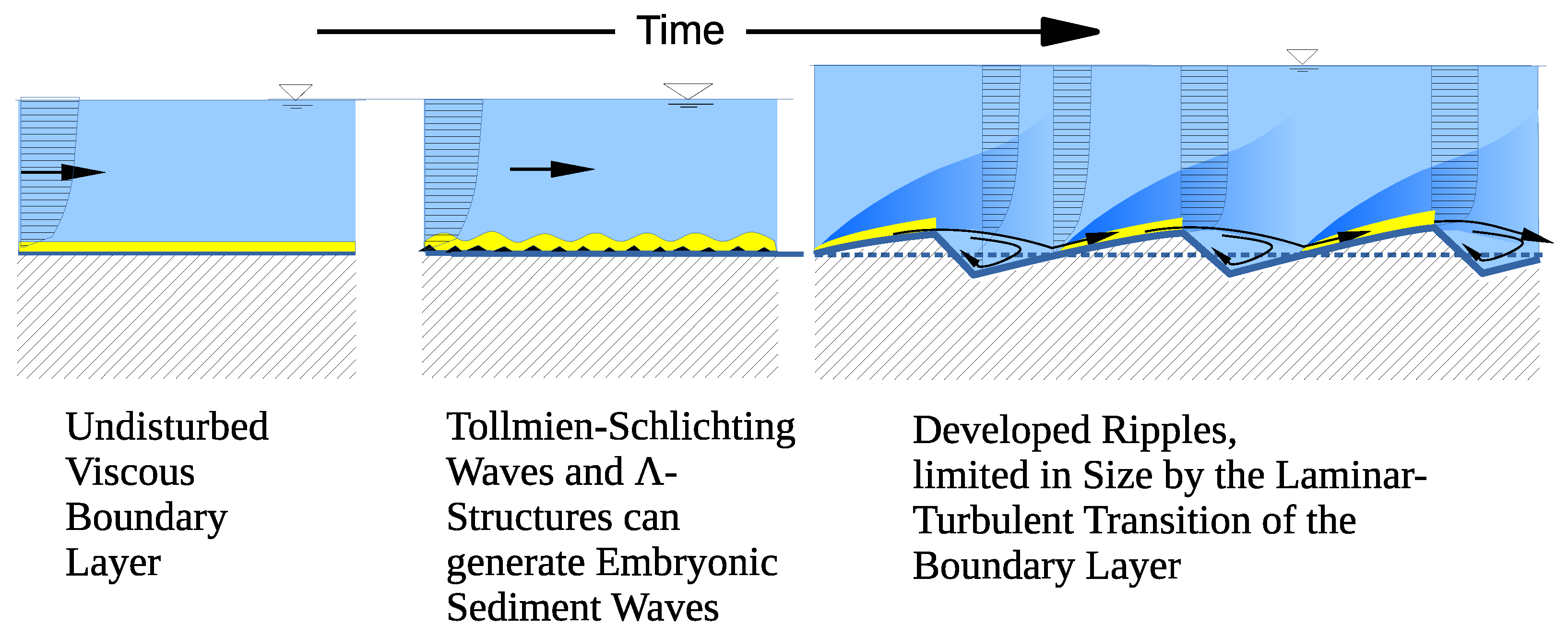
3. Rhythmic Structures of the Viscous Boundary Layer

In view of the widespread simultaneous occurrence of embryonic ripples in a developing ripple field with a uniform wavelength from a flat, even bed, wave-like instabilities of the fluid boundary layer, such as Kelvin–Helmholtz (KH) waves and Tollmien–Schlichting (TS) waves, can be considered as possible causes.

KH waves are generated at the shear plane of two parallel fluid streams (with different densities) that move at different speeds. An (effective) inflection point is present in the plane-normal profile of the plane-parallel velocity component, causing so-called inviscid (KH) instability, i.e., no viscosity is needed for disturbance growth in the given base flow. Even for the base flow, viscosity is just needed to slightly smooth the speed discontinuity between the streams to keep the shear finite. The fundamental KH-instability case of a ‘free shear layer’ has no limiting wall with no-slip condition, and thus can occur only at sufficient distance to a wall. For KH-instability to dominate, the shear layer must be thin, but this does not hold here because the distance between the bed and the moving sediment grains is distributed during their motion. Furthermore, observations show that the formation of ripples and their further development is definitely linked to viscous boundary-layer conditions with a wall, but we will show that inviscid instability plays an additional role during the very first ripple onset phase.

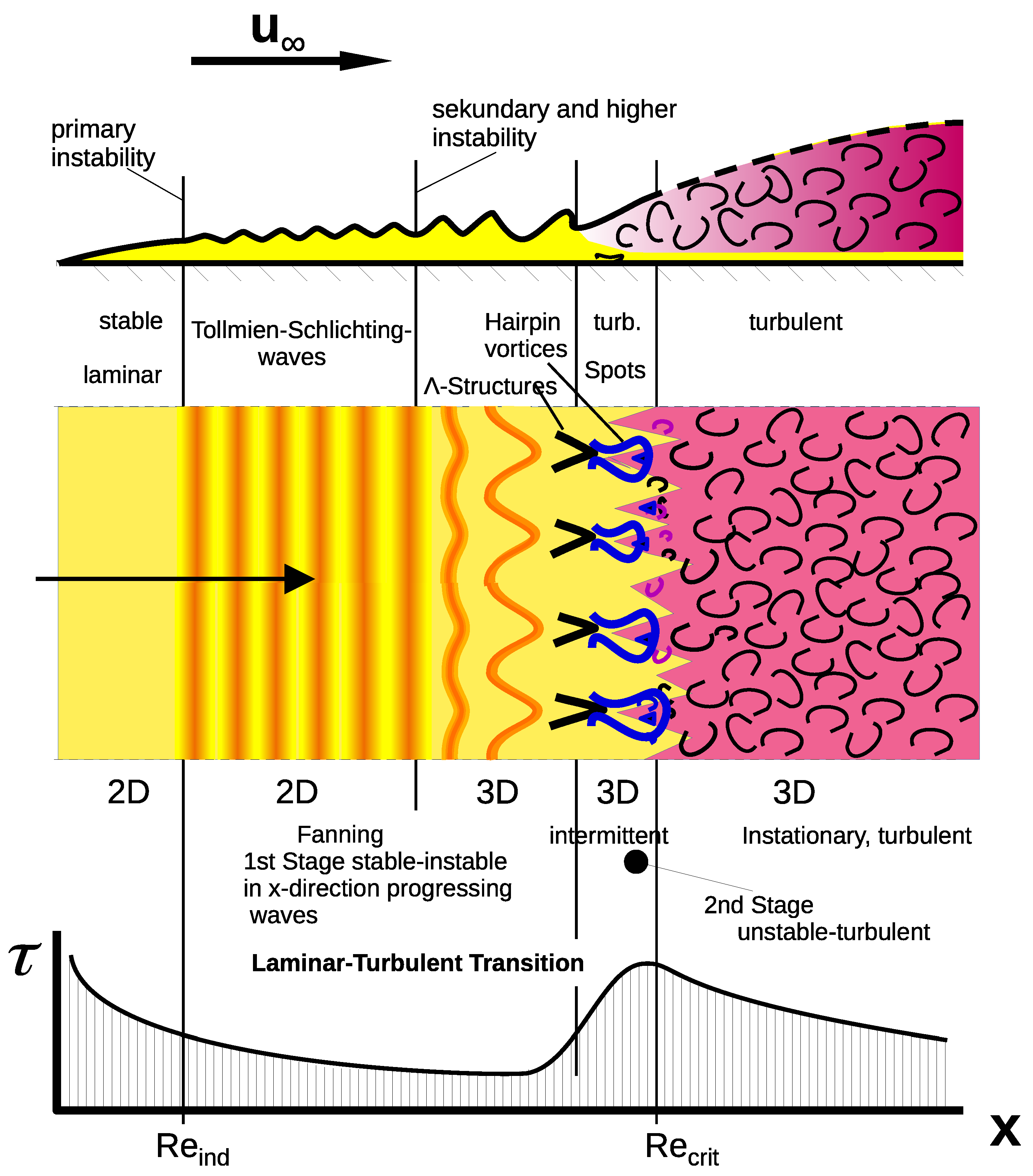
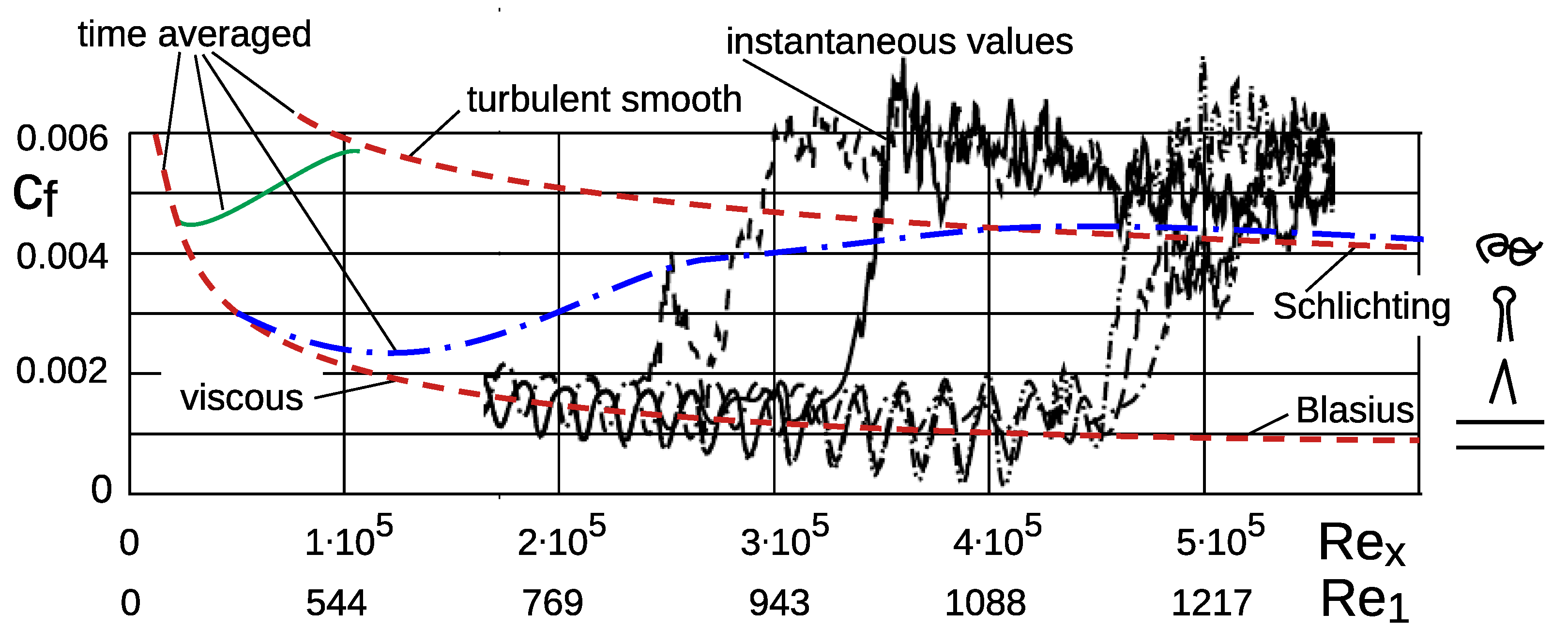
The Tollmien–Schlichting waves, on the other hand, are a phenomenon of the inherently viscous boundary layer. In 1929, Tollmien [28] recognized that instabilities can grow in the flat-plate boundary layer after a certain downstream distance, and Schlichting 1933 [29] and 1935 [30] (in [31]) carried out fundamental calculations. The base-flow velocity profile has no inflection point and, thus, inviscid instability is, for the standard flat-plate flow with constant flow speed, completely absent. The cause of instability is viscous effects within the disturbance flow. The waves, named after their discoverers, mark the beginning of the transition to turbulence in the boundary-layer flow. Their amplitude increases (exponentially) in streamwise direction. With increasing running length they become three-dimensionally deformed by secondary instability, i.e., they take on a serpentine-like course in the transverse direction and then develop into the so-called $\mathsf{\Lambda }$ vortices, from which the irregular turbulence finally emerges via the further intermediate step of hairpin-shaped vortices (see Figure 6).

The experimental proof of the two-dimensional TS waves was provided by Schubauer and Skramstad in 1947 [33].

TS waves occur on plates as well as in pipe and channel flows, and they progress in the direction of flow. In addition to the local Reynolds number, the transition is also influenced by whether the bed is flat, decreasing or increasing, i.e., whether the pressure is constant, increasing (retarded flow) or decreasing (accelerated flow) in streamwise direction. With regard to the initial formation of ripples, only the flat bed case is discussed here. In their further development, which is not the subject of this article, the acceleration of the flow along the windward ripple slopes plays an important role because it maintains the viscous flow for a longer period (see, in this regard, Zanke and Roland [34]).

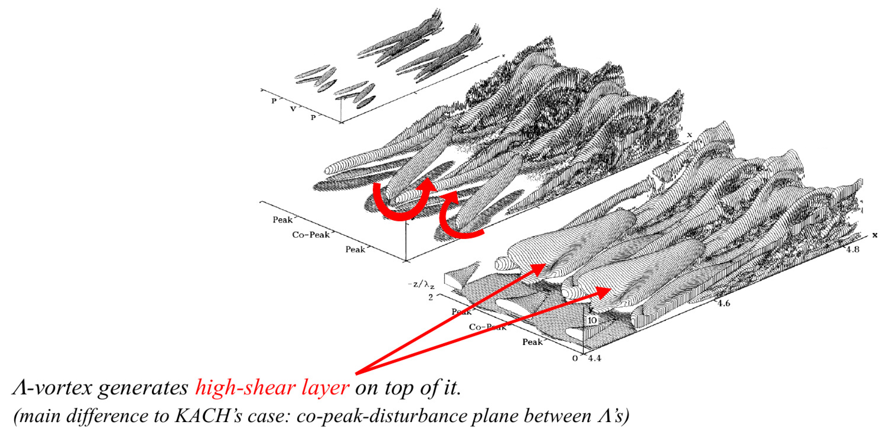
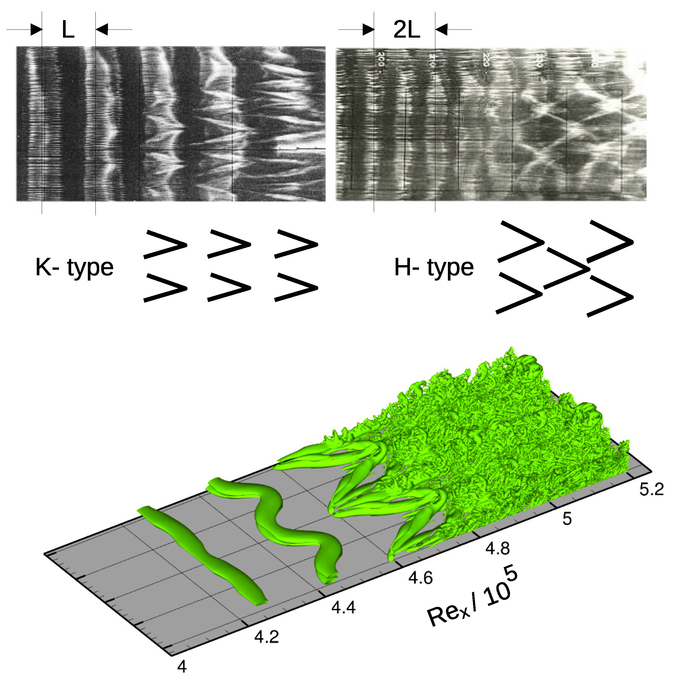
In Figure 7, the rhythmic boundary-layer phenomena are illustrated in different ways. The two upper images from Saric and Thomas 1984 [35] show a measurement-based visualization of two-dimensional TS waves and their transition into $\Lambda$-vortices. The picture below shows a result of numerical simulations by Kloker [36]. The $\Lambda$ vortices can occur in a so-called K-type (after Klebanoff) fundamental, or H-type (after Herbert) subharmonic scenario. In the K-type case, the $\Lambda$-shaped structures are arranged in line, with approximately the same sequence in flow direction as the TS waves. In the H-type case, the $\Lambda$ vortices are staggered. The natural transition is often via the K-type, boosted by tiny wall roughness. Two-dimensional TS waves are eventually rolls of discrete vortices with axes of rotation transverse to the flow, with same rotation sense as the base-flow vorticity, provided they have finite amplitudes.

The phenomena observed during the transition process from the laminar to the turbulent boundary-layer state are similar for the flat-plate boundary layer and the incipient, planar channel flow. The measured velocity fluctuations show the characteristic signal of the Tollmien–Schlichting waves in the area of the primary instabilities [37].

Figure 7. Transition from 2D Tollmien–Schlichting waves via 3D TS waves to K-type and H-type $\Lambda$ vortices, which then lead to turbulence. (Top): visualization according to Saric and Thomas 1984 [35] (in Kloker 2002 [36]). (Bottom): result of a numerical simulation by Kloker 1997 [38].

Figure 7. Transition from 2D Tollmien–Schlichting waves via 3D TS waves to K-type and H-type $\Lambda$ vortices, which then lead to turbulence. (Top): visualization according to Saric and Thomas 1984 [35] (in Kloker 2002 [36]). (Bottom): result of a numerical simulation by Kloker 1997 [38].

4. Process of Ripple Origin

According to the phase diagrams mentioned in Section 1, the ripple phase consistently only occurs in the hydraulically smooth range and in the transition range up to about $R{e}_d^{★}={\displaystyle \frac{u^{★}d}{\nu }}\approx 15$. It is therefore obvious that viscosity plays an important role in their formation and further existence, which is remarkable here because, as already mentioned, TS waves and $\Lambda$ vortices are also a phenomenon of viscous boundary-layer flow.

As early as 1957, Liu mentioned TS waves in the viscous boundary layer as a possible cause of ripple formation. However, he did not carry out any further analysis, and his hypothesis was not pursued by others, amongst other reasons because of the view that these boundary-layer instabilities, due to their relatively fast progression, could not leave regular “footprints” in the sediment (e.g., Hardtke 1979 [16]). The ripples progress much more slowly.

This article shows that and why such “footprints” are, in fact, possible, namely when the transport velocities of the upper bed load layer on the one hand and the propagation velocity of the TS waves and $\Lambda$ vortices on the other hand, at least approximately, coincide. Necessary conditions for ripple formation are as follows:

• The sediments at the bed are in motion when TS waves and $\Lambda$ structures occur.
• A sufficient portion of the sediments has transport velocities equal to or at least close to the travel velocity of the TS waves and the $\Lambda$ vortices, perhaps only temporarily, while the flow accelerates.
• Another condition is a height of the sediment accumulations such that the flow detaches here. Then, the incoming sediment load is deposited in the lee of the detachment and the embryonic ripples then migrate according to their own laws, i.e., independently of the governing boundary-layer phenomena, and each ripple forms its own boundary layer on each windward slope.

The legs of the $\Lambda$-vortices rotate and can thus leave the zigzag-shaped imprints on the bed. Figure 8 shows a reproduction from Kloker 2002 [36].

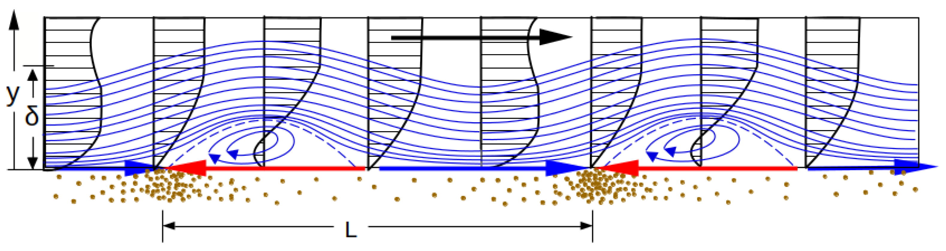
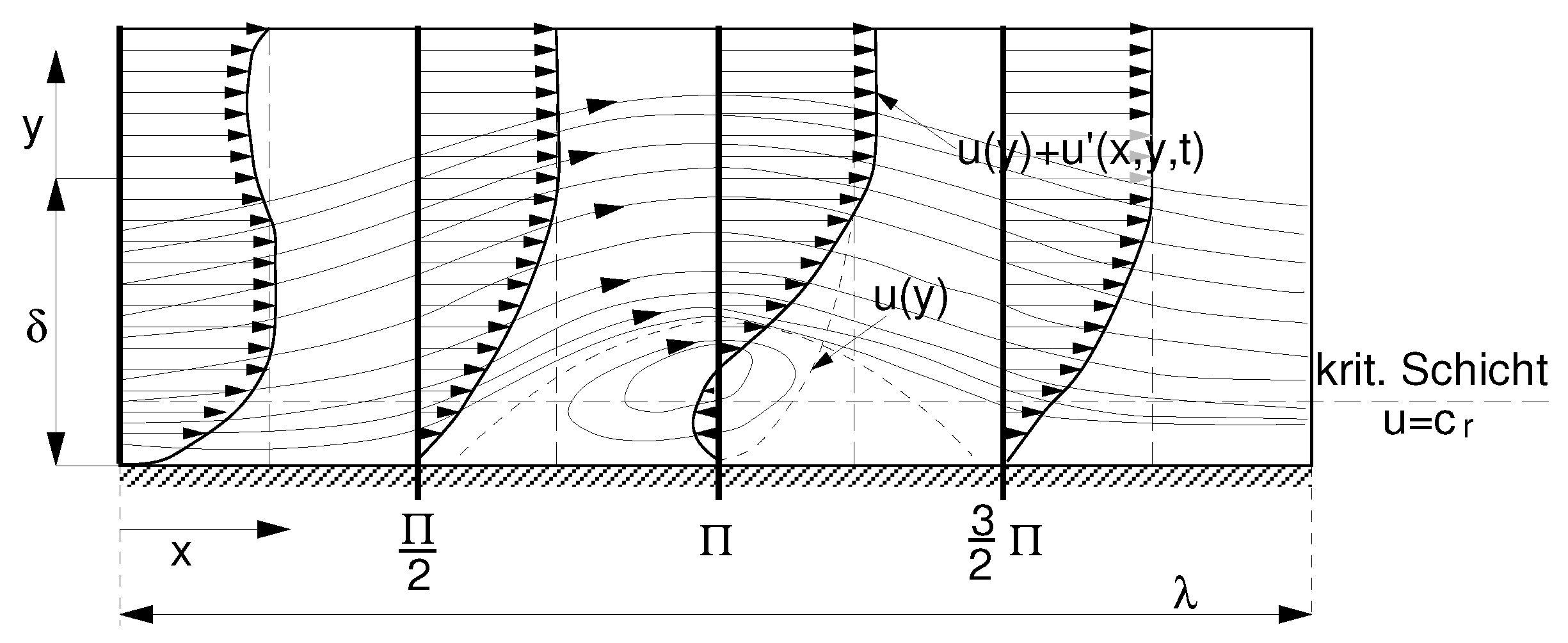
The legs of the $\Lambda$-vortices rotate, and can thus leave the zigzag-shaped imprints on the bed. Figure 8 shows a reproduction from Kloker 2002 [36]. In this way, the flow field of the TS waves and the $\Lambda$ vortices can arrange the moving sediment in such a way that it organizes itself into rhythmic sediment accumulations at intervals of one wavelength L each. Figure 9 shows currents computed by Schlichting 1935 [30] under TS waves, and Figure 10, further developed on this (see below), illustrates such a process. The flow directions at the bottom associated with the TS waves are indicated by blue and red arrows. It should be noted here that Figure 9 neglects the mean-flow deformation, which is generated nonlinearly by TS waves of finite amplitude. (It ultimately ensures that the wall-normal mean-longitudinal-velocity profile in a turbulent flow is fuller, with a larger wall gradient than in the laminar case). Taking this deformation into account, no instantaneous backflow occurs in the simple plate boundary layer as shown in the figure; however, this does occur when there is a mean-flow deceleration (or a streamwise pressure increase); see Kloker 1993 [39], 1997 [38], 2002 [36], 2024 [40], and Kloker and Fasel 1995 [41]. Such a deceleration occurs also when particles on the wall start to move in the approach flow, by the dragging effect of the wall shear. If the wall is suddenly set into some motion in the same direction as the external flow, the U(y)-velocity profile attains a local peak at the wall. From that peak, it first bends back near the wall before it merges with the former profile above. Thus, an inflection point is generated that causes additional (strong) inviscid instability. If the frame of reference for U(y) is moved with the wall velocity, to have relative zero velocity at the wall, a U(y)-profile with flow reversal shows off for some time. During that time, combined Tollmien–Schlichting/Kelvin–Helmholtz waves grow strongly, amplified by superposed viscous and inviscid instability. If the wall is slowly set into motion, no backflow appears at first, but an inflection point in U(y) is always present, its wall-normal position depending on the wall acceleration—the larger it is the higher the point sits with larger local dU/dy gradient, with increasing TS-KH growth rate. The effect is the same if the wall keeps zero velocity but the boundary-layer edge velocity is decreased—flow deceleration as standardly considered (Falkner–Skan flow with negative Hartree parameter; see, e.g., [39]). This scenario happens when sediment (the “wall” in the basic model) starts to be dragged by the flow, and boosts the origin of sediment ripples by transiently very strong growth of TS-KH waves, with somewhat shortened wavelengths, causing periodic flow reversal at grown amplitudes [40].

A similar effect is caused by the (particle) density, which increases due to the sediment loading of the fluid in the moving sediment layer near the wall. Thus, $du/dy$ is very small at the bottom of this layer, and increases towards the top, resulting also in inflectional velocity profiles. Therefore, Figure 10 characterizes the actual events in the case under consideration, including the qualitative inclusion of nonlinear disturbance components. We remark that even without instantaneous backflow, the TS waves can produce (initial) ripple crests, since the increased currents and shear stresses in the direction of flow alone are sufficient for this (blue arrows in Figure 10).

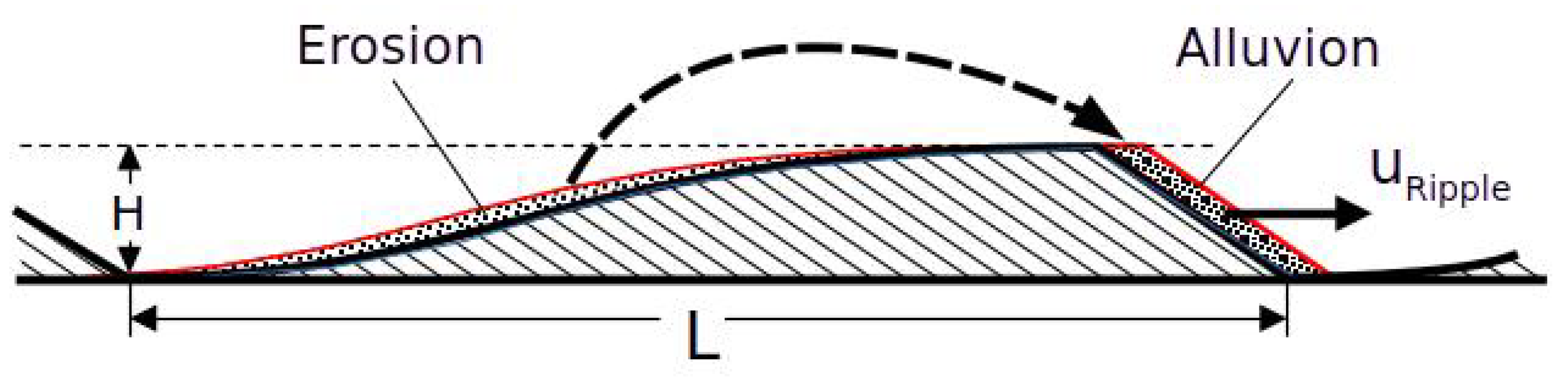
At the same speeds, the TS waves and the $\Lambda$-vortices are stationary from the point of view of the moving sediment particles. As a result, the effect of the flow under these boundary-layer phenomena is maximal compared to the case of different speeds of sediment and wave propagation. As soon as accumulations of a few grain sizes in height are created with flow detachments, the embryonic ripples migrate according to the laws of ripple mechanics. Grains accumulate in the lee behind the crests, and only begin to move again when they are uncovered on the windward slope during ripple migration. This effect on the moving sediment is illustrated in Figure 11. As a condition for flow separation at the embryonic crests, Hardtke 1979 [16] mentions “a few grain diameters” and Venditti et al. 2005 [17] report 1 to 2 grain sizes for the initial ripple heights based on their observations. They also cite a finding by Williams and Kemp 1971 [42], according to which detachments occur when $u^{★}H/\nu >4.5$, which can be read here as

$$u_{c,i}^{★}H/\nu >4.5$$

(5)

with $u_{c,i}$ = critical shear stress velocity for ripple formation.

For $\mathbf{H}=\mathbf{2}\mathit{d}$, this criterion is satisfied in all the experiments in Table 1. From this moment on, new boundary layers form along the newly created windward slopes, as illustrated in Figure 12 on the right.

Under these conditions, the further formation of the ripples can take place as follows:

• Behind the mini-ridges, the flow separates and then reattaches to the bed a little further downstream. Beginning with the reattachment of the flow, a windward slope with its own boundary layer is created.
• The development of these sub-boundary layers is connected to the further development of the embryonic ripples until they reach their final size. Zanke and Roland 2021 [34] describe that, and how this further development is determined by the laminar–turbulent transition of the viscous boundary layers along the windward slope.
• Due to the rapid increase in the shear stress at the transition to turbulence in the boundary layer (see Figure 6), the ripple length is limited by the maximum possible length of the viscous boundary-layer flow along the windward slopes. The rise increases the transport capacity far beyond the incoming sediment, thus forcing local erosion and a flow separation over the erosion zone.

In the following sections, the relevant boundary-layer conditions are examined in more detail and analyzed for their compatibility with the ripple hypothesis formulated here.

5. Conditions for Matching Velocities of TS Waves and Sediment Particles

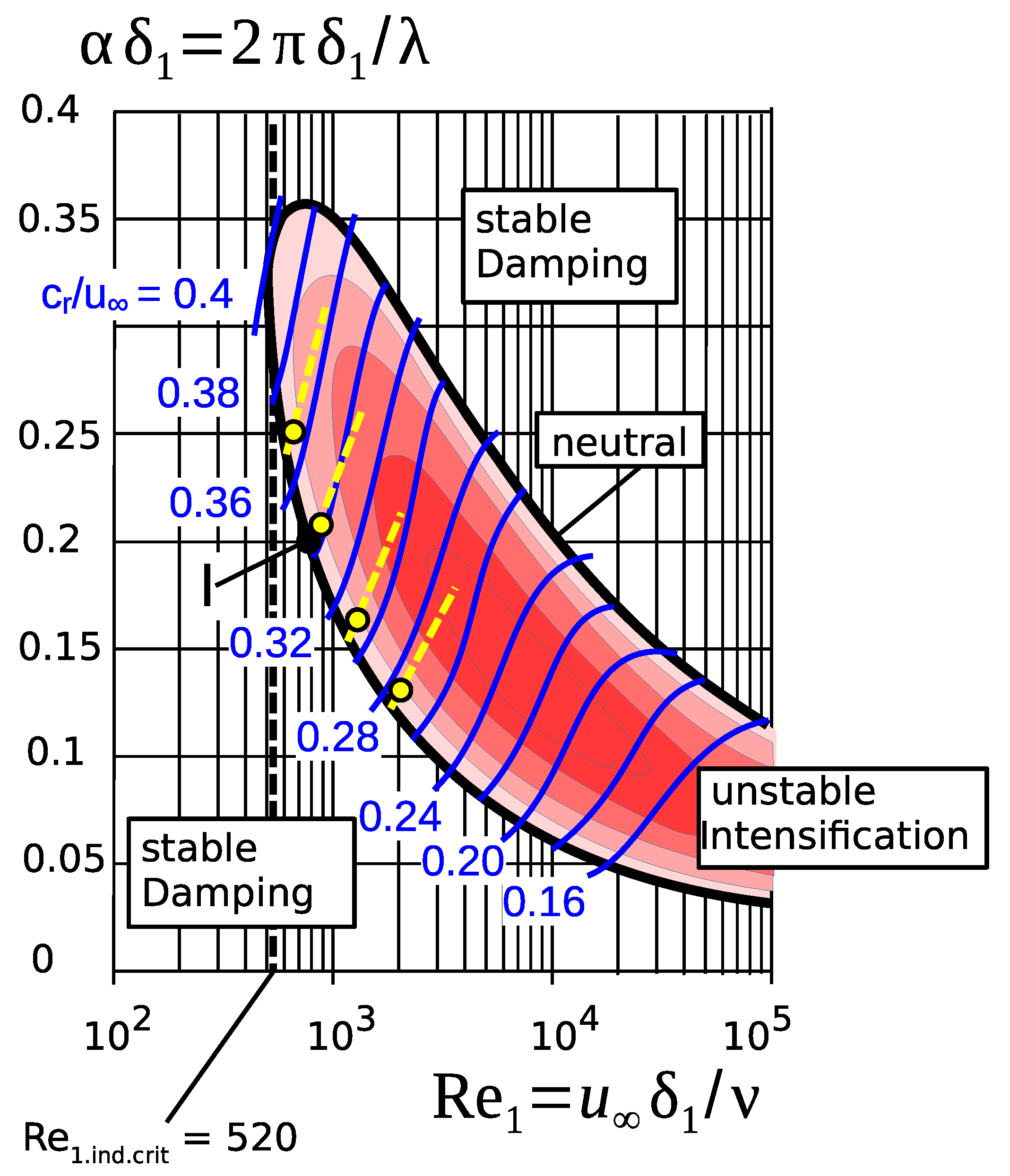
The speed of the TS waves and the $\Lambda$ vortices can be seen in Figure 13. The figure shows the Tollmien indifference curve according to an evaluation by Obremski et al. 1969 [43], along which TS waves are neither damped nor amplified, as well as areas with damping and amplification. The diagram shown is for the so-called temporal model with temporal instead of spatial amplification because easier to compute. The neutral line is identical for both models. The physically correct spatial intensification (rate: $-{\alpha }_i$) can be obtained from the temporal one using the relation according to Gaster: $(-{\alpha }_i)$~${\omega }_i/c_{group}$, where $c_{group}$ is the group velocity which is approximately equal to the real phase velocity here. The wave phase velocities of both models are approximately the same, as are the wavelengths, and the diagram can be used directly here. Furthermore, the relative speed of progress $c_r/u_{\infty }$ of the boundary-layer structures is indicated, as is the intensity of the red coloration, with its degrees of amplitude intensification (modal, exponential growth rate) rising to the center. For the outer flow, its mean velocity is understood to be decisive here and $u_{\infty }=u_m$ is set. For the left branch of the indifference curve, it follows that

$$0.4⪆c_r/u_m⪆0.2.$$

(6)

where $c_r$ is the wave progression speed (Figure 13).

Figure 13. Indifference curve for the boundary layer on a plate with a longitudinal flow according to Tollmien [28] 1929 in a calculation according to Obremski et al. 1969 [43]. Blue: relative migration velocities $c_r/u\infty$ of the boundary layer waves. Figure 9 shows the computed streamlines ($\alpha =2\pi /L$) for point I. In increasing color intensity: strengthening intensities for the boundary layer instabilities. The yellow dashed lines fulfill Equation (20), and the yellow dots mark the approximate position where the TS waves can generate the first ripples (for more details, see Section 9.

Figure 13. Indifference curve for the boundary layer on a plate with a longitudinal flow according to Tollmien [28] 1929 in a calculation according to Obremski et al. 1969 [43]. Blue: relative migration velocities $c_r/u\infty$ of the boundary layer waves. Figure 9 shows the computed streamlines ($\alpha =2\pi /L$) for point I. In increasing color intensity: strengthening intensities for the boundary layer instabilities. The yellow dashed lines fulfill Equation (20), and the yellow dots mark the approximate position where the TS waves can generate the first ripples (for more details, see Section 9.

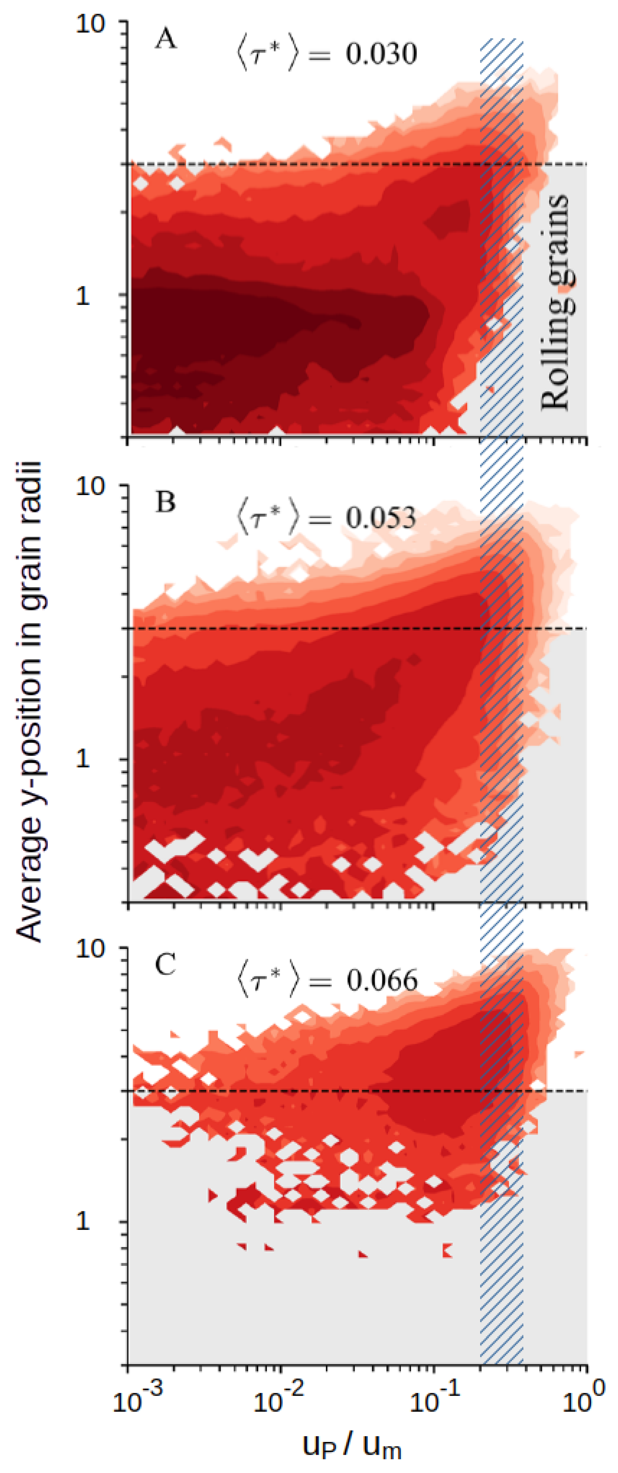
Relative particle velocities $u_p/u_m$ can occur in the same order of magnitude. However, the further condition of sufficiently uniform sediment transport arises from the observations of Hardtke 1979, and also of Venditti et al. 2005. This initially occurs in intermittent phases at its onset with just supercritical shear stresses. With increasing flow stress, homogenization occurs. Benavides, Venditti, and Ven 2023 [44], on the basis of recent laboratory experiments with glass beads (see Figure 14), note:

“Rolling grains are found to have a large range of possible velocities, with the maximum likelihood occurring at low values of velocity (A), pointing to its on-off intermittent nature. On the other hand, saltating grains, whose centers lie three grain radii or more above the bed, tend to follow a velocity profile similar to that of the fluid, with a larger mean velocity and a smaller range of observed fluctuations around it (C)”.

It should be noted here that in the model consideration of a purely moving wall (without sediment), the effective boundary layer outer velocity is the difference between the actual outer velocity and the wall velocity, and thus lower; the phase velocities would then be somewhat lower in this model, but this is practically lost in the bandwidth.

The hatching in Figure 14 indicates the range $0.2<u_P/u_m<0.4$. However, it can also be seen that there is a clear spectrum of grain velocities starting from the point where the critical shear stress is exceeded.

It can be seen from the observations by Benavides, Venditti, and Ven 2023 [44] that grain velocities exist in the range of the propagation velocities of TS waves and $\Lambda$-vortices, even if the beginning of the movement is only slightly exceeded; however, in insufficient amounts and only locally and intermittently. As the dark red area in the upper part of the image shows, the majority of the grains moved are much slower. From about ${\tau }^{★}/{\tau }_c^{★}\approx 2$, corresponding to $u^{★}/u_c^{★}\approx 1.4$, the majority of the particles moves at a significantly more uniform speed (see lower sub-image with ${\tau }^{★}/{\tau }_c^{★}\approx 2.2$). This is also consistent with observations by Hardtke (see Table 3.1 on Hardtke p. 69). Accordingly, the conditions for ripple formation are given at approximately ${\tau }^{★}/{\tau }_c^{★}\approx 2$.

The same (or at least similar) speeds of TS waves and $\Lambda$ vortices on the one hand, and a sufficient amount of sediment particles in motion on the other, are thus possible. The flow fields of the TS waves and the $\Lambda$ vortices can therefore group the sediment particles in wavelength intervals, thus causing the formation of ripples. It is already sufficient if this condition exists temporarily during the acceleration phase of the flow. In the laboratory tests of Hardtke as well as in those of Venditti et al., ripples occur during the ramp-up of the flow. As soon as the first ridges exist, they migrate according to their own laws, as mentioned above.

6. Condition for the Occurrence of TS Waves and $\Lambda$ Vortices

The lowest $R{e}_1$ number for a neutral or amplified wave in flat-plate flow is

$$R{e}_{1,\mathrm{crit}}=520$$

(7)

with

$$R{e}_1={\displaystyle \frac{u_{\infty }{\delta }_1}{\nu }}={\displaystyle \frac{u_{\infty }}{u^{★}}}{\displaystyle \frac{{\delta }_1}{d}}R{e}^{★}.$$

(8)

If one refers to the length x instead of the displacement thickness ${\delta }_1$, then the smallest $Re$ number for indifferent, i.e., neither damped nor excited, TS waves are obtained as $R{e}_{x,c}\approx$ 91,000. With increasing $Re$ values, i.e., with increasing flow velocity $u_{\infty }$ and/or increasing run length x, or increasing boundary layer thickness $\delta$, the transition to turbulence, in which the ripples arise, begins at a critical Reynolds number $R{e}_c$ (or higher for lower wavenumbers/frequencies that have significant integral amplification).

In the literature, the route via TS waves is referred to as the natural route, in contrast to the so-called bypass that skips the TS waves. Depending on which wavelength/frequency prevails, the indifferent region shifts towards larger $R{e}_c$ (see Figure 13). Then, the (neutral) waves become longer, and the relative propagation velocities $c_r/u_{\infty }$ become smaller. Some examples of possible transitions are shown in Figure 15. The essential message here is that (i) the peak values of the flow resistance (i.e., also of the shear stresses) are increased by TS waves, (ii) the transition to turbulence can occur at different Reynolds numbers, and (iii) strong external turbulence and/or larger wall roughness can shift the transition to smaller Re values than shown in Figure 13.

Depending on the nature of the external turbulence and the roughness of the wall, the transition of the viscous wall flow to turbulence occurs sooner or later, as already mentioned. Both relatively abrupt and comparatively slow transitions have been observed.

For the formation of ripples, only the first phase of the transition is essential, in which regular structures arise that can cause regular “imprints” in the moving sediment layer. These are the TS(-KH) waves and $\Lambda$ vortices with their own internal currents.

Table 2. Some relationships of the viscous boundary layer (localized values).

Boundary layer thickness	$\mathit{\delta }={\mathit{\delta }}_{99}=\frac{5\mathit{x}}{\sqrt{\mathit{R}{\mathit{e}}_{\mathit{x}}}}$
Displacement thickness	${\delta }_1={\displaystyle \frac{1.72x}{\sqrt{R{e}_x}}}=0.344\delta =R{e}_1{\displaystyle \frac{\nu }{u_{\infty }}}=1.72\sqrt{R{e}_x}·{\displaystyle \frac{\nu }{u_{\infty }}}$
Resistance coefficient	$c_f=2{({\displaystyle \frac{u^{★}}{u_{\infty }}})}^2={\displaystyle \frac{0.644}{\sqrt{R{e}_x}}}={\displaystyle \frac{1.14}{R{e}_1}}={\displaystyle \frac{{\tau }_w^{★}{\rho }^{\prime }gd}{1/2u_{\infty }^2}}$
Reynolds numbers	$R{e}_1={\displaystyle \frac{u_{\infty }{\delta }_1}{\nu }}=1.72\sqrt{R{e}_x}=0.344{(R{e}_d^{★}{\displaystyle \frac{\delta }{d}})}^2,R{e}_x={\displaystyle \frac{u_{\infty }x}{\nu }}$
u-profile	${\displaystyle \frac{u_y}{u^{★}}}={\displaystyle \frac{u^{★}y}{\nu }}$

summarizes some of the essential relationships for understanding. For decelerated boundary layers, the thickness parameters are slightly larger, the critical Reynolds number is smaller, the amplification rates are larger, the wavelengths are slightly shorter, and their bandwith is larger.

7. Effect of Wall Roughness

The above $R{e}_c$ values initially apply to smooth wall surfaces. For rough walls, the critical $R{e}_c$ values can be lower, as mentioned above, i.e., the beginning of the transition to turbulence can occur earlier (see Figure 15). In principle, this also applies to sediment beds.

In the present case with a moving sediment bed, the walls are not smooth, but consist of sand, thus raising the question of the influence of roughness on the transition of the boundary layer. Hall 2021 [48] remarks

“It should also be noted that even in flows where Tollmien–Schlichting waves are possible the absence of flow unsteadiness to trigger the waves could also lead to the roughness instability playing a crucial role.” and further

“Perhaps one of the most surprising results of our investigation is that the roughness instability occurs at small wave amplitudes long before the motion induced by the wall is governed by interactive boundary-layer theory.”

• Kuester & White 2015 [49] with respect to roughness effects emphesize

“Reshotko & Leventhal 1981 measured streamwise velocity over a flat plate with sandpaper roughness. In their experiment, the distributed roughness displaced the boundary layer away from the wall. They also measured low-frequency oscillations that were later identified as transient, non-modal, non-exponential growth (Reshotko  2001).   Kendall   (1981) used glass beads to create a distributed roughness field and noticed the same displacement of the boundary layer away from the wall.  Corke, Bar-Sever & Morkovin 1986 measured enhanced growth of T–S waves in the presence of sandpaper roughness in a flat plate boundary layer. The roughness, which was located downstream of the T–S wave neutral stability curve, modified the growth rate of T–S waves. Transition occurred through the breakdown of these T–S waves rather than an instability initiated by the roughness."

• Floryan 1997 [50] cites

“Feindt  1957 used sand grains of different sizes and concluded that for $Re=uk/\nu <120$ the roughness has no influence and the transition takes place at the same location as on the smooth surface. Here k denotes the grain size, u stands for the velocity of the oncoming flow, and ν denotes the kinematic viscosity.”

• and also at Floryan

“Corke et al. 1986 carried out experiments using sand paper to represent distributed roughness. They reported (i) that it is the low-inertia fluid in the valleys between the grains that responds to free-stream disturbances, (ii) once Tollmien–Schlichting waves appear, they grow faster (although the reason is unknown) as compared to the smooth- wall case, and (iii) there is evidence of roughness-induced three-dimensionalization of the wave fronts leading to earlier secondary instabilities.” as well as

“Reshotko & Leventhal 1981 found that distributed roughness in the form of sand paper thickens the boundary layer and moves the essentially undeformed Blasius profile outward. The important growth of disturbances occurs in frequencies lower than those for which Tollmien–Schlichting waves are unstable. The amplification seems to be driven by the local wake profile at the crest of distributed roughness elements (Reshotko 1984).”

8. Limit of Ripple Emergence

From the above, in particular from Feindt’s 1956 finding [51], it can be seen that wall roughness has no influence on the transition to turbulence, as long as $\mathit{Re}={\mathit{u}}_{\infty }\mathit{d}/\mathbf{\nu }<\mathbf{120}$, and that the transition then takes place at about the same position as over a smooth surface. This initially applies to immobile walls.

From the literature on sand waves, it can be seen that ripples in the transport system of sand and water on Earth can only exist in the range $R{e}_d^{★}⪅15$. Thus, the limiting values correspond to $Re=u_{\infty }d/\nu <120$ and $R{e}_d^{★}=u^{★}d/\nu ⪅15$. The latter criterion is based on observations of sediment motion. This correspondence can also be verified using the general velocity profile in Zanke and Roland 2020 [52] (see Equation (31)). For $R{e}_y^{★}=15$, the ratio $u_y/u^{★}\approx 8$ is obtained, which is 120/15 for all $y>d$, or for $y=\delta =nd$ and $n>1$.

Table 3. Values $R{e}_{d,ci}^{★}$ of the experiments by Hardtke, Kühlborn, and Venditti et al.

	d	$\mathit{\nu }·{10}^6$	${\mathit{u}}_{\mathit{c},\mathit{i}}^{\mathit{★}}$	${\mathit{Re}}_{\mathit{d},\mathbf{ci}}^{\mathit{★}}$
	mm	m2/s	m/s	-
Hardtke	0.15	1.08	0.0176	2.44
Kühlborn	0.16	1.03	0.0173	2.69
Venditti et al.	0.5	1	0.024	12

summarizes relevant data. Ripples can therefore occur if

$$d⪅15{\displaystyle \frac{\nu }{u_{c,i}^{★}}}$$

(9)

For example, $u_{c,i}^{★}=0.026$ m/s for $d=0.6$ mm, and thus at a water temperature of 20 °C, then is $R{e}_d^{★}=15.6$.

For sand in air flows, the conditions with regard to $u_{c,i}^{★}$ are somewhat different. Due to the much greater mass differences between the sand grains and the fluid, the grains experience considerable ballistic bouncing soon after the first grains begin to move. These accumulate energy from the flow during their flight, which they partially release in their rebound from the bed, thereby setting other grains in motion in a chain reaction. This reduces ${\tau }_c^{★}$ to about half the value determined by Shields in 1936 [19] for sand in water flows. It is not known to what extent the bouncing grains affect the formation of TS waves and $\Lambda$ vortices. However, it can be assumed (subject to future research results in this regard) that the critical grain size for ripple formation is already reached here at lower values of $u_{c,i}^{★}$ without the roughness directly leading to disorderly turbulence, instead of rhythmic TS waves. If, in this sense, $u_{c,i}^{★}=u_c^{★}$ is assumed for air flows, then for $d=0.6$ mm; for example, $u_c^{★}\approx 0.48$ m/s as the threshold value, $R{e}_d^{★}\approx 19$ is obtained for the end of the ripple generation.

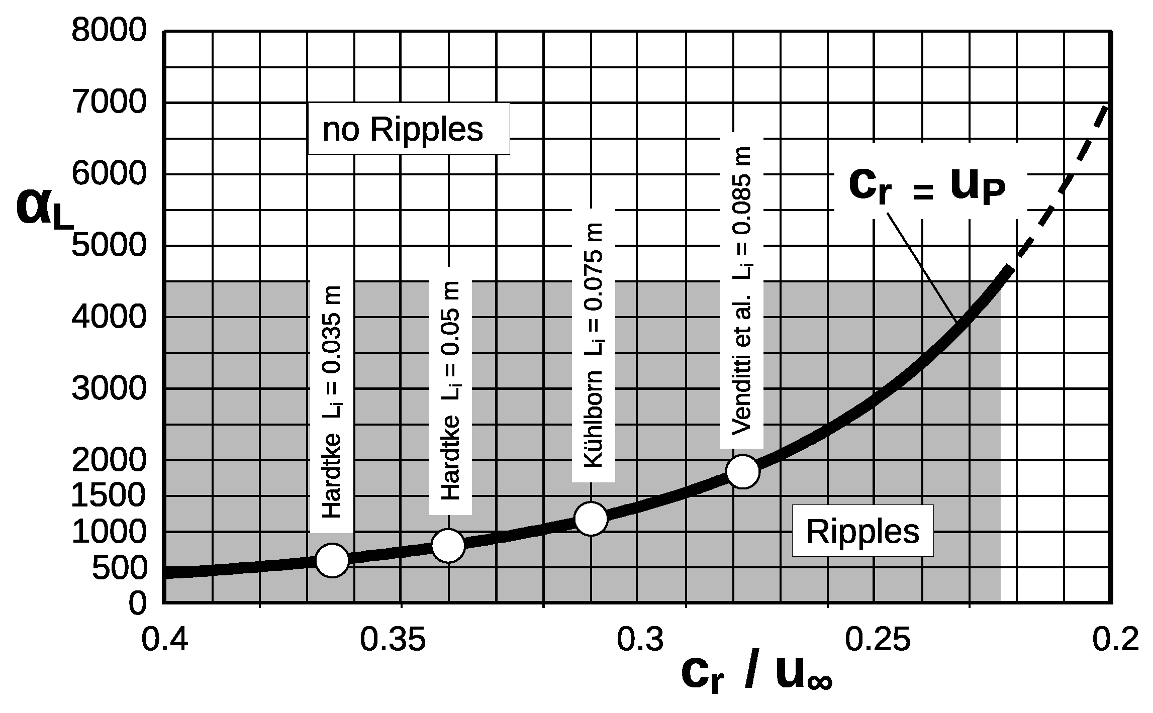
The embryonic ripples are still relatively modest in height, which is why the acceleration of flow on the windward slopes can be neglected. Then, according to [34], the maximum possible length of the ripple is $L_{max}\approx 4500\nu /u^{★}$, i.e., here

$$L_{i,max}\approx 4500\nu /u_{c,i}^{★}$$

(10)

It should be noted here that values of up to around $L_{max}\approx$ 30,000$\nu /u^{★}$ can be achieved due to the accelerated flow over well-developed ripples ([52]). From Figure 13, ${\alpha }_L$ by regression can be expressed as ${\alpha }_L\approx 9.5{(c_r/u_m)}^{1.07}$, from which one obtains the following for the limit of the relative wave propagation speed:

$${\left({\displaystyle \frac{c_r}{u_m}}\right)}_{min}\approx 0.22.$$

(11)

Therefore, due to $u_p=cr$, the smallest relative particle velocity at which ripples occur (Figure 16) is

$${\left({\displaystyle \frac{u_p}{u_m}}\right)}_{min}\approx 0.22.$$

(12)

9. Initial Ripple Length

9.1. Lengths Determined from Measurements

Unfortunately, both Hardtke and Venditti et al. report only the values that occurred at the target speed of the experiments, such as flow velocity, shear stress, and shear stress rate, but not the values at the time of the first ripple appearances.

From his measurements, Hardtke takes a distance between the $\Lambda$ vortices and, thus, also the length $L_i$ of the initial ripples for the sediment he uses, $d=0.15$ mm, of

$$L_i\approx 750{\displaystyle \frac{\nu }{u^{★}}}=750{\displaystyle \frac{\nu }{\sqrt{{\tau }_{c,i}^{★}{\rho }^{\prime }gd}}}$$

(13)

with a range of

$$600⪅L_i^{★}=u^{★}{L}_i/\nu ⪅1600,$$

(14)

where the respective final test speed and an average ripple length of $4.3$ cm are applied. In Experiment IV by Hardtke, for example, ${\tau }^{★}=2.2{\tau }_c^{★}$ (${\tau }_c^{★}\approx 0.065,u_{c,i}^{★}=0.0176$ m/s) and further $u_{final}^{★}=0.0188$ m/s. With reference to $u_{c,i}^{★}$ instead of $u_{final}^{★}$, $L_i$ can be related to the moment of the start of movement, whereby the value 750 changes to ≈700. For its 5 cm long initial ripples, this gives ${\displaystyle \frac{u_{c,i}^{★}{L}_i}{\nu }}=L_i^{★}=815$, and for the $3.5$ cm long initial ripples, $L_i^{★}=570$.

In experiment ‘A’ by Venditti et al. with $u_{m,final}=0.501$ m/s$(u_{final}^{★}=0.027)$ and $d=0.5$ mm, the dominant length of the initial ripples is about $L_i=8.2$ cm with a bandwidth of $6\mathrm{cm}⪅12$ cm. For this experiment, therefore, $L_i^{★}=1970$. Here, a significantly different disturbance frequency is obviously dominant compared to the experiments by Hardtke. At the somewhat lower flow velocities in experiments ‘B’ ($u_{final}^{★}=0.028$ m/s) and ‘C’ ($u_{final}^{★}=0.022$ m/s), the initial lengths are similar. In all three cases, $u_{c,i}^{★}=0.024$ is reached or exceeded in the target state.

9.2. Wavelengths of TS Waves and $\mathsf{\Lambda }$ Vortices

From Figure 13, it follows for the wavelength of neutral, i.e., neither damped nor excited, TS waves and similar to the $\Lambda$-vortices

$$L={\displaystyle \frac{2\pi }{\alpha {\delta }_1}}{\delta }_1.$$

(15)

The displacement thickness ${\delta }_1$ of the viscous boundary layer is described by

$${\delta }_1=R{e}_1{\displaystyle \frac{\nu }{u_{\infty }}}$$

(16)

and, thus,

$$L={\displaystyle \frac{2\pi }{\alpha {\delta }_1}}R{e}_1{\displaystyle \frac{\nu }{u_{\infty }}}.$$

(17)

This can be expressed in terms of the shear rate $u^{★}$ as

$$L={\displaystyle \frac{2\pi }{\alpha {\delta }_1}}{\displaystyle \frac{u^{★}}{u_{\infty }}}R{e}_1{\displaystyle \frac{\nu }{u^{★}}}$$

(18)

With $u^{★}/u_{\infty }=\sqrt{c_r/2}$ and $c_r=0.664/\sqrt{R{e}_x}=0.76/\sqrt{R{e}_1}$, for the wavelength, we finally obtain

$$L={\displaystyle \frac{4.75}{\alpha {\delta }_1}}\sqrt{R{e}_1}{\displaystyle \frac{\nu }{u^{★}}}.$$

(19)

According to the aforementioned observations, the formation of ripples due to amplified TS waves or $\Lambda$ vortices does not begin on the neutral curve, but in the area of the amplification at slightly higher $Re$ numbers, which are estimated here to be $1.2R{e}_{1,neutral}$. Then,

$$\begin{array}{|c|}\hline L_i={\alpha }_L{\displaystyle \frac{\nu }{u_{ci}^{★}}}\\ \hline\end{array}$$

(20)

applies with ${\alpha }_L={\displaystyle \frac{5.7}{\alpha {\delta }_1}}\sqrt{R{e}_{1,i}}$. Structurally, this is in line with Hardtke’s empirical findings according to Equation (13). The initial ripple lengths are obviously as follows:

• Not directly dependent on the grain size, but only indirectly via the grain size dependence of the onset of sediment motion.
• As in observations, independent of a flow depth, since this does not appear in the derivation.
• The above derivation is therefore fundamentally applicable to any sediment in any fluid.

Following Equation (20), the initial lengths depend on the one hand on the ratio $\nu /u_{c,i}^{★}$ and, on the other hand, on ${\alpha }_L$. Thereby, $u_{c,i}^{★}$ is a function of ${\rho }^{\prime },g$ and d (see Equation (1) and Figure 2). The value of ${\alpha }_L$, i.e., the ripple-inducing combination of $R{e}_1$ and $\alpha {\delta }_1$, is controlled by the coincidence of the grain velocity and the wave velocity. The combinations of $\sqrt{R{e}_{1,i}}/\alpha {\delta }_1$ to be fulfilled (

Table 4. Combinations of $\sqrt{R{e}_{1,i}}$ and $\alpha {\delta }_1$ to be fulfilled for the observed initial ripple lengths.

	$\sqrt{{\mathit{Re}}_{\mathit{c},\mathit{i}}}/\mathit{\alpha }{\mathit{\delta }}_1$	${\mathit{\alpha }}_{\mathit{L}}$
Hardtke	100	570
Hardtke	143	815
Kühlborn	220	1254
Venditti et al.	346	1972

, see also Table 1) are as follows.

In Figure 13, the locations for which Equation (20) is fulfilled are indicated by dashed yellow lines. The curves are assigned from top left to bottom right in the order given in Table 1 (Hardtke, Hardtke, Kühlborn, Venditti). The yellow dots indicate the probable position of the ripple occurrence. In the case of (initially) decelerated boundary-layer flow, the stability diagram (see Figure 13) is extended upwards and to the left, and the two upper yellow lines to Hardtke also fit because the combination values according to Table 1, then tend to be in the smaller range (around 100). It should also be noted that the location within the unstable area in the stability diagram depends on several factors, such as the perturbation background (turbulence level) in the flow, and the perturbation receptivity of the boundary layer.

10. Incipient Ripples on Other Planets

Ripples and dunes are also observed on other planets; for example, on Mars and on Saturn’s moon Titan. However, the gravitational conditions and densities of sediment and fluid, as well as the fluid viscosities, are significantly different. Consequently, other lengths of initial ripples are also to be expected. For both planets, developed ripples reach significantly greater lengths. In this respect, this is also to be expected for initial ripples. Note that, according to the instability-theory model, the wavelengths scale with the boundary-layer thickness, i.e., they are inversely proportional to the square root of the unit Re-number which is basically $U\rho /\mu$.

Table 5. Some characteristic data of the planets and the initial ripple length using Equation (20), exemplified for a grain size $d=0.4$ mm. The right column shows the calculated length relations $L_P/L_E={(\nu /u_{c,i}^{★})}_{Planet}/{(\nu /u_{c,i}^{★})}_{Earth}$.

Planet	g (m2/s)	${\mathit{\rho }}^{\prime }$	$\mathit{\nu }$ (m2/s)	${\mathit{u}}_{\mathit{c},\mathit{i}}^{\mathit{★}}$	$\mathit{\nu }/{\mathit{u}}_{\mathit{c},\mathit{i}}^{\mathit{★}}$	$\frac{{\mathit{L}}_{\mathit{P}}}{{\mathit{L}}_{\mathit{E}}}$
Earth (sand–water)	9.81	1.65	$1\times {10}^{-6}$	0.023	$3.96\times {10}^{-5}$	1
Earth (polystyrene–water)	9.81	0.03	$1\times {10}^{-6}$	0.0047	$2.1\times {10}^{-4}$	5.3
Mars (drippable fluid) *	3.78	1.04	$4\times {10}^{-5}$	0.025	$1.6\times {10}^{-3}$	40
Titanium (dripable fluid) *	1.35	0.85	$5\times {10}^{-6}$	0.011	$4.45\times {10}^{-4}$	11.2
Earth (sand–air)	9.81	2160	$1.5\times {10}^{-5}$	0.38	$5\times {10}^{-5}$	1
Mars (sand–air) **	3.78	$1.45\times {10}^5$	$5.4\times {10}^{-4}$	2.65	$2\times {10}^{-4}$	4
Mars (sand–air) ***	3.78	$1.45\times {10}^6$	$5.4\times {10}^{-3}$	10.73	$5\times {10}^{-4}$	10
Titanium (sand–air) ****	1.35	188	$1.5\times {10}^{-5}$	0.06	$2.5\times {10}^{-4}$	5

Note: * $g,\rho ,\nu$ aus Lapotre et al. 2017 [15]; **$g,\rho ,\nu$ aus Lapotre et al. 2016 [53] for ${\rho }_{Luft}=0.02{\mathrm{kg}/\mathrm{m}}^3$; ***$g,\rho ,\nu$ aus Lapotre et al. 2016 [53] für ${\rho }_{Luft}=0.002{\mathrm{kg}/\mathrm{m}}^3$; ****$g,\rho ,\nu$ aus Charnay et al. 2015 [54] and aus Risbeth et al. 2000 [55] In the case of sediment driven by air or other gases, ${\tau }_{c,impact}=0.5{\tau }_c$ was set due to the saltation-impact effect.

shows the corresponding basic data and the range of the computed initial ripple lengths for some cases. The numerical example applies to $d=0.4$ mm. $u_{c,i}$ and $\nu /u_{c,i}$ are given, as well as the multiple of the resulting initial ripple length compared to the Earth, separately for droppable liquids and gases.

While ripples formed in the Earth’s waters reach only a few decimeters, they can be several meters long on Mars in the salt brine and in the cold (approx. $-190 °$C) liquid methane of Saturn’s moon Titan. Larger initial ripple lengths than on Earth also form there under wind. According to Table 5, the initial lengths there are also significantly greater than on Earth. In addition, the table shows that the initial ripples for the example of sand $d=0.4$ mm under wind on Earth are somewhat longer than under water, with the factor $5/3.96\approx 1.26$.

Due to the requirement for the same transport velocity of the sediments and the phase velocities of the boundary-layer waves, a further variation in length may occur, depending on where the point of origin lies in Figure 13.

11. Further Development After Emergence

In the further development of ripples that have already formed, a detachment zone of increasing height grows behind the first crests. The total length of the ripple now consists of the length of the detachment until it reattaches to the bed and, from there, of the length of the windward slope. For a typical steepness $H/L\approx 1/11$, the length of the windward slopes is then about 60% of the total length [34]. Because of the low heights H of embryonic ripples, the length of the detachment zone is marginal for these.

A convex windward slope rises from the point where the current reattaches to the bed. This is due to the shear stress distribution on Figure 6: because of the initially decreasing shear stress behind the resulting crest lines, sediment continues to accumulate until the shear stress along the windward slopes is locally sufficient to transport the incoming sediment (including the sediment from local erosion). The resulting acceleration of the current along the windward slopes reduces turbulence, allowing the windward slopes to become longer than they would be without this effect (Zanke and Roland 2021 [34]).

12. Results and Conclusions

Ripples are a phenomenon of sediment motion. They often form the surface of granular sediments, and thus influence the sediment loads and roughness to the current. They develop simultaneously over wide areas with a largely uniform length, even in previously completely flat sediment beds. This paper addresses the question of how this is possible and provides a plausible explanation: if regular, wave-like disturbances occur in the near-bottom flow and their propagation velocity approximately matches the transport velocity of the sediments on the bed, with sufficiently strong sediment transport, then this flow can organize the sediment particles into embryonic ripples at intervals of one wavelength each. It is shown that and under which boundary conditions this can be the case with Tollmien–Schlichting waves, initially merged with Kelvin–Helmholtz-type waves, and the resulting $\Lambda$-vortices. This also explains why ripples only occur under hydraulically smooth flow conditions. The solution presented here also explains earlier observations (e.g., by Hardtke 1979 [16] or Venditti et al. 2005/2006 [17,56]) that, in laboratory experiments and under natural conditions, the flow velocity of the driving fluid is not decisive for the formation of ripples, because the ripples already form during the acceleration of the flow when $\tau \approx 2{\tau }_{c,Shields}$. It must therefore only reach a flow velocity at which $u^{★}\ge u_{c,i}^{★}$ occurs, even if only temporarily during the flow acceleration. During this initial phase, the sediment (the wall) is pulled into motion, translating into an instantaneous effective deceleration of the boundary-layer flow, leading to additional inviscid KH-type instability, thus boosting the TS(-KH) waves’ growth.

An important hydrodynamic aspect is the fact that the ripple formation causes the boundary-layer flow along the windward slopes not to turn into turbulence, and instead successive viscous (or laminar) boundary-layer conditions remain near the wall. However, in addition to these, there is an energy loss at each ripple crest due to flow separation.

For a description of ripple length, the term $L=factor·\nu /u^{★}$ is often taken (e.g., Hardtke 1979 [16] or Rubanenko et al. 2022 [57]. Here, by an analytical deduction, this term is verified.

13. Remark

This paper is part of a Textbook on Physical Fundamentals of Sediment Motion in preparation by the Author.