Abstract
Reliable coastal and offshore sediment transport data is a requirement for many engineering and environmental projects including port and harbour design, dredging and beach nourishment, sea shoreline protection, inland navigation, marine pollution monitoring, benthic habitat mapping, and offshore renewable energy (ORE). Novel sediment transport numerical modelling approaches allow engineers and scientists to investigate the physical interactions involved in these projects both in the near and far field. However, a lack of confidence in simulated sediment transport results is evident in many coastal and offshore studies, mainly due to limited access to validation datasets. This study addresses the need for cost-effective sediment validation datasets by investigating the applicability of four new suspended load validation techniques to a 2D model of the south-western Irish Sea. This involves integrating an estimated spatial time series of suspended solids concentration () derived from acoustic Doppler current profiler (ADCP) acoustic backscatter with several in situ water sample-based datasets. Ultimately, a robust spatial time series of ADCP-based was successfully calculated in this offshore, tidally dominated setting, where the correlation coefficient between estimated and directly measured is 0.87. Three out of the four assessed validation techniques are deemed advantageous in developing an accurate 2D suspended sediment transport model given the assumptions of the depth-integrated approach. These recommended techniques include (i) the validation of 2D modelled suspended sediment concentration () using water sample-based , (ii) the validation of the flood–ebb characteristics of 2D modelled suspended load transport and using ADCP-based datasets, and (iii) the validation of the 2D modelled peak over a spring–neap cycle using the ADCP-based . Overall, the multi-disciplinary method of collecting in situ metocean and sediment dynamic data via acoustic instruments (ADCPs) is a cost-effective in situ data collection method for future ORE developments and other engineering and scientific projects.
1. Introduction
Reliable coastal and offshore sediment transport data is a requirement for many engineering and environmental projects, including port and harbour design [1], dredging and beach nourishment [2,3], sea shoreline protection [4], inland navigation [5], marine pollution monitoring [6], benthic habitat mapping [7], and offshore renewable energy (ORE) development projects including wave [8,9], tidal [10,11,12], and wind energy [13,14]. With the increased demand in marine resources for offshore renewable energy developments [15,16] a comprehensive understanding of sediment transport regimes on a local and regional scale in a coastal and offshore environment is imperative. The installation of infrastructure on the seabed, for example, wave and tidal energy converters and wind turbine foundations, alters wave propagation, flow patterns, and sediment circulation [12,17,18,19,20,21]. Specific oceanographic parameters effected may include turbulence, and mixing and vertical stratification, subsequently impacting sediment resuspension, sedimentation, temperature change, nutrient transport, and substrate availability [22,23]. In the far field, subsequent physical impacts to the marine environment could be detrimental, causing beach width reduction [24], or could be beneficial, aiding coastal protection [9,25]. The nature of this impact depends on the local oceanographic regime, the type and size of the ORE development, and lay-out configurations.
In the near field, these changes have the potential to alter marine biogeochemistry including marine life behaviour, phytoplankton dynamics, and benthic habitats [13,23]. Evidently, baseline information is critical to qualify and quantify changes that may occur in the sediment transport system as a result of these developments. Additionally, developing baseline risk maps to identify areas of regional stability may aid developers in choosing low-risk zones in terms of scour (e.g., Coughlan et al. [26]). The determination of cable burial depths may also be aided through the knowledge of seabed mobility potentials [27]. Furthermore, it is imperative to simulate near-seabed velocities to quantify seabed shear stress and scour in order to mitigate infrastructural instability [28,29].
Numerical modelling is an excellent tool that can be used to gather this qualitative and quantitative baseline (natural regime) information on hydrodynamics, waves, and sediment transport dynamics in coastal and oceanic regions [8,30,31,32]. It can also be used to simulate the responses of the physical environment imposed by the installation of these marine structures [8,11,12,25,33,34]. State-of-the-art sediment transport numerical modelling techniques takes many forms including one-dimensional (1D) [35], two-dimensional (2D) [12], two-dimensional vertical (2DV) [36,37], three-dimensional (3D) [38], and smoothed-particle hydrodynamics (SPHs) [39] modelling. Across many environments (fluvial, coastal, and offshore), the assumptions underlying the depth-integrated (2D) modelling approach are commonly accepted and adopted when considering several project variables, including environmental conditions, model scale, model resolution, computational power, project timelines, and project budget [26,31]. On the other hand, 3D models are becoming increasingly more feasible with the advancement of technology such as high-performance computing [40]. Regardless, a common challenge to all techniques is the paucity of in situ sediment data to calibrate and validate these numerical modelling techniques.
In many sediment transport studies only the underlying hydrodynamic and wave models are validated using in situ field data [8]. Where field sediment properties such as median grain size, sorting, grain density, etc., are available they act as inputs into these models, yet modelled sediment transport outputs are generally not validated. This may be due to limited data availability and associated high costs for data collection campaigns. Few studies have managed to quantify bed load transport through the use of bed level changes and sand wave migration characteristics derived from geophysical datasets [12,38,41]. Comparably, a limited number of studies have attempted to validate suspended sediment transport variables using optical backscatter sensors (OBSs) and transmissometers [11,42,43,44]. For example, a study off the coast of Anglesey, in the Irish Sea [11], validates a two-dimensional (2D) suspended sediment transport model using estimated suspended sediment concentration () from a Sequoia 100-X LISST (Laser In Situ Scattering and Transmissometry), calibrated via a number of water samples. This validation process was limited to one location, a 4-day observational dataset, and visual observation comparison techniques. From the published time series plot, modelled concentrations are clearly underestimated during peak spring flow. However, a spread is evident in the measured values as all depths are recorded and included in the validation process; this invokes an interpretation difficulty in the comparison against these measured values with the depth-averaged modelled values. Conclusively, there is clear paucity of investigation into the development of suspended sediment transport model validation techniques. Increased validation would ultimately improve the accuracy of numerical models, which is imperative for the acceleration of cost-effective engineering projects with a sustainable and environmental focussed ambition.
This study will focus on potential validation techniques for the suspended sediment transport variables of 2D numerical models. The conventional (laboratory-based) method for measuring suspended solids concentration () is the most accurate, yet sole direct sampling via sediment traps or water sampling is expensive and time-consuming. It requires a high sampling time at the observation site, collecting samples at different timestamps and water column depths in order to capture the full dynamics of the system. It requires a high processing time and does not provide a full spatial and temporal time series.
On the other hand, the use of optical backscattering sensors (OBSs) and transmissometers overcome this spatial and temporal resolution issue with the capability of producing a time series of high-frequency measurements of suspended mass concentration [45]. Although this captures the variable nature of in the water column, the calibration of these instruments is highly complex as the response function of the OBS depends on grain size and is nonlinear with the concentration of suspended solids [45,46]. Additionally, optical sensors are especially sensitive to biological fouling problems [47,48].
Alternatively, acoustics sensors which are less susceptible to effects of biological fouling, such as acoustic Doppler current profilers (ADCPs), are typically used to measure ocean currents and velocity profiles, yet also record acoustic backscattering intensity which is directly related to [49,50,51]. The estimation of from this recorded echo intensity using the sonar equation is not a straightforward process yet has been under development for many years [49,50,52,53,54,55,56,57]. This method development is predominately focussed on fluvial environments where high mass concentrations dominate [50,51,54,55,58], with few applications in high-energy coastal systems [59]. This method of estimation depends on multiple environmental factors, including water temperature, salinity and pressure, and instrument characteristics such as operational frequency, power, and transducer size. Early studies account for beam spreading and water absorption in the calculation of transmission losses but exclude corrections for the attenuation from suspended particles and non-spherical spreading in the transducer near field. Other studies incorporate these factors [60,61,62]. In general, the application of this method has proven very successful in many fluvial and coastal environments across the globe [63,64,65] and is gaining increasing acceptance amongst coastal engineers and sedimentologists.
This method comes with various limitations which have been outlined in previous studies [57,59]. For example, the choice of instrument is highly important in terms of frequency in order to fully capture expected particle size in the water column [57,66]. Generally, higher frequency ADCPs have the ability to detect finer grain sizes in the water column [67], yet they have lower maximum blanking distances and ranges (along the beam path) [50]. For example, a 300 kHz ADCP has a maximum range and blanking distance of 300 m and 1 m, respectively, yet a 1000 kHz ADCP has a maximum range and blanking distance of 25 m and 0.2 m, respectively [50]. When used in an offshore environment, a combination of ADCP frequency, environmental considerations, such as water depth and particle size distribution, and other measurement needs (whether the ADCP is being used to measure ocean currents and waves simultaneously) must be considered on a case-by-case basis, especially when using single-frequency systems. Additionally, single-frequency instruments cannot differentiate between changes in concentrations versus changes in particle size distribution (PSD) over the deployment time period. Therefore, in fluvial environments, where PSD is highly variable, this must be taken into consideration during the conversion process. Multi-use frequencies can help overcome this issue. The calibration of such systems is under investigation [56], yet this approach increases complexity and cost.
There is a lack of investigation into the applications and limitations of ADCP-based in offshore tidal-dominated environments where mass concentrations in the water column are far less compared to fluvial environments, and non-cohesive medium to very coarse sands dominate the seabed. Nevertheless, the success of this method in fluvial and estuarine environments shows a high potential for its successful application offshore. If ADCP-based can be adequately quantified in this way in tidally dominated shallow shelf sea environments, it could be established as a very cost-effective multi-purpose instrument for the simultaneous collection of meteorological, oceanographic, and sediment dynamic parameters for numerical model validation.
Consequently, in this paper we address the following two hypotheses:
- can be adequately estimated from the echo intensity recorded by a 300 kHz acoustic Doppler current profiler (ADCP) in a shallow shelf sea environment.
- The spatial time series of ADCP-based can be used as a validation technique for a 2D (suspended) sediment transport numerical model.
From these hypotheses, this study aims to do the following:
- Using equations developed by previous authors, estimate from the acoustic amplitudes recorded by a 300 kHz ADCP deployed in a tidally dominated shallow shelf setting characterised by complex hydrodynamics and a non-cohesive seabed substrate (Figure 1).
- Explore different model validation techniques to validate the suspended load transport and SSC aspect using a combination of direct sampling and ADCP-estimated .
- Evaluate the applicability and advantages of the new validation techniques presented and provide best practice recommendations for future studies.
This study focuses on south-western Irish Sea (Figure 1C). The highly complex hydrodynamics and sediment transport pathways in this region have been studied extensively in recent years [26,30,68,69,70,71]. In the Irish Sea, tidal flow is the main physical driver of seabed mobility whereby the dominant tidal constituents are M2 and S2 [30,71]. The flood tidal flow enters the Irish Sea from the Atlantic Ocean through the St Georges Channel and the North Channel moving northwards and southwards, respectively. The northward flow circulates around a degenerate amphidromic point pinpointed on the east coast of Ireland, near Courtown (Figure 1C); the southward flow circulates around an amphidromic point in the North Channel. The two flood tidal waves intersect in the central Irish Sea, generating a symmetrical tidal zone and a bed load parting zone [30]. The ebb tide is in the reverse direction. In the western Irish Sea, a series of coast parallel active sand banks, including Arklow Bank (Figure 1C), are located at approximately 20–40 m water depth, rising to only a couple of metres below sea level [68]. These bedforms influence the regional and local hydrodynamics and morphodynamics, whereby complex sediment transport pathways connecting offshore sand banks to offshore independent sediment wave assemblages have been identified [68]. Two of these offshore independent sediment wave assemblages are identified in Figure 1C. Although tidal flow is the principal driver of sediment mobility in the Irish Sea, waves are shown to be the dominant process driving sediment mobility in coastal areas and in some regions where these offshore sand banks are present [26].
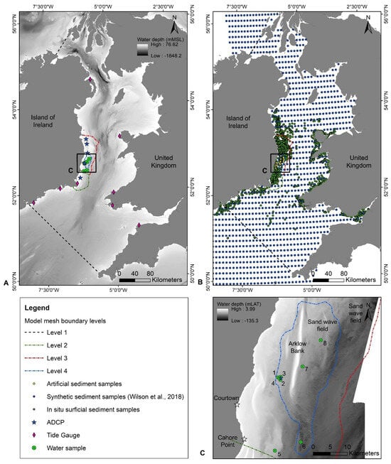
Figure 1.
(A) Site map displaying the area of interest, numerical model mesh boundary levels, and numerical model validation and calibration points; (B) three sediment sample datasets used in the sediment transport model: (i) manually added artificial samples, (ii) synthetic samples from Wilson et al. [72], and (iii) in situ surficial sediment samples; (C) study site displaying water sampling and ADCP stations. (Bathymetry source: A: [73] C: INFOMAR [74]).
Section 2 outlines the methodology used in this study, including ADCP deployment and water sample collection, background theory of the sonar principle and equations used in the estimation of from ADCP, numerical model development, and novel seabed substrate map development. Section 3 provides an overview of results including water sampling, ADCP-based , a comparison against ADCP-based and measured datasets, and the outcome of four tested model validation techniques using a combination of directly measured and ADCP-estimated time series. Section 4 and Section 5 provide a discussion and conclusion of project results, respectively.
2. Methods
2.1. ADCP Deployment and Water Sample Collection
To analyse suspended solids concentration () in the south-western Irish Sea, 66 water samples were obtained across 8 sampling stations onboard the RV Celtic Voyager during three offshore survey campaigns (CV20010, CV20036, and CV21034) in September/October 2020 and December 2021. These survey campaigns were carried out under the ‘Mobility of Sediment Waves and Sand Banks in the Irish Sea (MOVE)’ project. A Teledyne Workhorse Sentinel 300 kHz acoustic Doppler current profiler (ADCP) was also deployed inside a trawl-resistant bottom mount frame during this project from 27 September to 14 October 2020 at 52.722°, −6.028° (Figure 1). Half of these water sampling stations (stations 1 to 4) (Figure 1) provide in situ measurements for the estimation of an time series derived from echo intensity recorded by the ADCP. The use of water samples in this way determined their collection methodology in terms of location, timing, and water depth of sample.
The timing of each sample was targeted at peak ebb and peak flood tide. This was to ensure the presence of a relatively high amount of suspended sediment in the water column during sampling times, corresponding to relatively high current speeds. To determine these tidal times pre-survey, a time series of currents and water levels was extracted for each of the eight water sampling stations from the North East Atlantic (NEATL) hydrodynamic model held by the Marine Institute. The NEATL is an implementation of the three-dimensional Regional Modelling System (ROMS) and can provide an estimate of tidal times across the Irish Sea. Harmonic analysis was carried out on these datasets from which a tidal prediction over the survey time-frame was produced. These were further analysed to derive desired estimated tidal times.
Stations No. 1–4 were taken as close as possible to both the deployed ADCP and to the estimated peak flood–ebb tidal time. The setup of the ADCP deployment (e.g., avoidance of the surface marker buoy), drifting of the vessel due to strong tidal currents, vessel safety procedures, and limitations of the NEATL model predictions had to be considered at each sampling time and location. Water sampling was carried out using a rosette sampler containing 12 five-litre Niskin bottles. Each water sample was taken at a different water depth corresponding to each ADCP bin. The dimensions of the ADCP setup are presented in Figure 2. As shown, the first water sample was taken approximately 3.81 m above the seabed and at 1 m intervals from here. From each five-litre bottle, a two-litre sample was retained and tested for total suspended solids (TSS). The same methodology was carried out for stations 5 to 8.
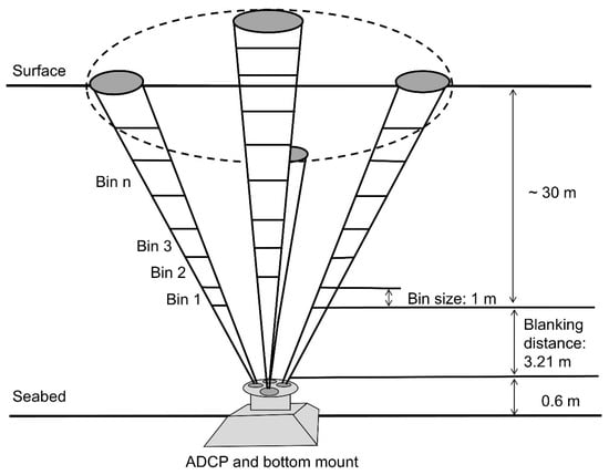
Figure 2.
Schematic diagram of the setup of the upward-looking Teledyne RDI Workhorse Sentinel 300 kHz acoustic Doppler current profiler (ADCP) at the study site.
2.2. ADCP Derived SSC
The method of estimating from echo intensity recorded by an ADCP employs the following formula which is based on the sonar equation for the sound scattering of small particles [55,59,75]:
where and are the intercept and slope, respectively, determined by the regression of ADCP relative acoustic backscatter () with known measured on a semi-log plane in the form of [55,59,75], which is as follows:
Therefore, in order to derive an estimated time series for throughout the water column at one location, the echo intensity () (counts) recorded along one beam (in this case, beam 4) of the deployed ADCP was processed and converted to relative backscatter () (decibels) through the following equation [54,67];
where is the reverberation level and accounts for two-way travel transmission losses. Based on the sonar equation [76], the reverberation level is given as follows:
where is the source level and is the target strength of suspended sediment. When measuring with an ADCP, the reverberation level can be given as follows [53]:
where is the measured returned signal strength indicator (RSSI) amplitude recorded by the ADCP for each bin along each beam, in counts. is the amplitude seen by the ADCP in the absence of any signal or the baseline amplitude. is the RSSI slope which is a factor specific to each beam of each instrument used to convert counts to decibels. In this case the for beam 4 is 0.4048. This value was received from the manufacturer. The equation used for the correction of the two-way transmission loss () is given as follows [55]:
where the term accounts for the loss due to spreading and accounts for the loss due to absorption, whereby is the absorption coefficient for sediments and is the absorption coefficient due to water.
is the slant range and varies with height from the sensor () and is calculated here as follows [52]:
whereby is the depth cell number of the scattering layer being measured, is the blank after transmit (m), is the transmit pulse length (m), is the depth cell length (m), is the beam angle, is the speed of sound in the water used by the ADCP, and is the average sound speed from the transducer to the range cell that depends on the depth and is computed by means of the equation by Mackenzie [77] and is calculated for each bin at each timestep using the following equation:
where is the temperature in degrees Celsius (measured by the ADCP at the transducer at each timestep), the is salinity in parts per thousand (measured by the ADCP at the transducer at each timestep), and is the depth in metres (varies according to bin depth).
Additionally, the spreading loss is different in the near and far fields. For this, the R critical () was calculated as follows [67]:
where represents the Rayleigh distance (m), which depends on the frequency used. The Rayleigh distance for RDI Workhorse Sentinel 300 kHz is 0.87 m, which is taken from Mullison [53]. This value does not vary but is fixed for each bin and each timestep.
From this, the near field correction for spreading loss () is calculated by using the following [78]:
where , therefore varies for each bin and timestep. Next, the transmission loss due to the absorption of seawater , depends on a variety of environmental conditions and the frequency of the ADCP [53]. This is calculated for each timestep as follows [79]:
where is the typical pH value of seawater, T is temperature in degrees Celsius measured by ADCP, is salinity (psu) measured by the ADCP, is the maximum depth (km), is boric acid, is magnesium sulphate, and is the frequency of the ADCP (kHz). The resulting correlate very well with the absorption coefficient given in Mullison [53], 0.068 dB/m, which was calculated for a 300 kHz ADCP in a 4 °C water temperature and 35 ppm salinity. This study uses a water temperature of 14.7 °C, salinity of 35 ppm, and a 300 kHz ADCP, giving an value of 0.087 dB/m. In order to calculate we use Urick’s [80] equation, which gives the following coefficient for the attenuation of acoustic energy by sediment (expressed in dB/cm):
where is the dimensionless volumetric sediment concentration (SSC divided by sediment density), is the wave number, λ, is the wavelength in cm, is the specific gravity of the sediment, is the mean sediment radius in cm, is equal to , and is equal to , in which is equal to , is , f is frequency in hertz (Hz), and is the kinematic viscosity of the water in stokes [55]. The calculated concentration for 1 mg/L is 0.000482 dB/m. This shows a very good agreement with the value determined in the study by Baranya and Józsa [51].
Once the is calculated, values are input back into Equations (1) and (2) to derive an estimated spatial time series of .
2.3. Numerical Modelling
A dynamically coupled two-dimensional (2D) hydrodynamic and sediment transport model was developed using DHI’s MIKE 21 suite of tools [81,82,83] in order to investigate the complex feedback sediment transport system between offshore sand banks and offshore independent sediment wave fields identified in previous studies [68]. An integral part of this model development is the need to understand the relationship between bed load and suspended load sediment transport in this dynamic system. The validation of the bed load sediment transport component of this model is addressed in Creane et al. [68] and Creane et al. [69]. Utilising all available datasets for this region of interest, Creane et al. [68] shows that the direction of residual bed shear stress and residual tidal current align well with the direction of sand wave migration derived from repeat multi-beam bathymetry datasets, whereas Creane et al. [69] adds confidence to the bed load transport component of the model by comparing volume change in time-lapse bathymetry datasets to volume change in simulated bed level changes. This study focusses on developing validation techniques for the suspended sediment transport variables of this model. The techniques developed will further increase the confidence level of our model feeding directly into future local and regional work, but they will also be applicable to a broad-spectrum of model applications in other geographical regions. Section 2.3.1 and Section 2.3.2 describes the coupled hydrodynamic and sediment transport modelling approach used.
2.3.1. HD Modelling
Two attempts at developing a high resolution, medium-scale, 2D hydrodynamic model of the south-western Irish Sea was carried out using the DHI’s MIKE 21 suite of tools [81,82,83] in an effort to produce a computationally efficient model for the area of interest. Both the model domain and unstructured, flexible mesh were kept consistent for both models, whereby the south and north boundaries extended eastwards from the east coast of Ireland at Courtown (52.530835°, −6.215659° to 52.479936°, −5.81943°) and Wicklow Head (53.096108°, −6.036121° to 53.084429°, −5.640141°), respectively. The water level boundary conditions were driven by (i) the DHI Global Tide Model [84] and (ii) the MIKE 21 FM hydrodynamic model developed by Coughlan et al. [26]. After multiple calibration iterations and output examinations, it was decided that these local models failed to capture the full complexity of hydrodynamics in this region which were previously identified in Creane et al. [30] and Creane et al. [68]. As a result, the hydrodynamic model covering the entire Irish Sea developed in Coughlan et al. [26] was used in this study. This 2D depth-averaged model resolves the Navier–Stokes equations using a finite-volume scheme. The north and south open boundaries are driven by a 15 min interval water surface elevation time series based on tidal constitutents from the DHI Global Tide Model [84], with a spatial resolution of . The model boundaries were set as fixed, but water level boundary conditions varied spatially along the boundary to represent the difference between eastern and western sides of the Irish Sea. The astronomical constituents used to generate the boundary conditions included the major semidiurnal tidal constituents (M2, S2, N2, and K2) and diurnal constiuents (K1, O1, P1, and Q1). The model simulation timestep is 30 s.
This model was updated with additional geophysical datasets; additionally, a new refined mesh was implemented and a new validation point was utilised. An outline of the original hydrodynamic model is presented in Coughlan et al. [26] whilst new updates and modifications to the model setup includes the following:
- An addition of 16 bathymetric datasets to increase the accuracy and resolution of the seabed topography in the south-western Irish Sea.
- A total of 15 of these datasets were collected via the INFOMAR (Integrated Mapping for the Sustainabe Development of Ireland’s Marine Resource) programme between 2011 and 2017 onboard a range of survey vessels. These datasets were provided at a spatial resolution between 2 m and 5 m and vertical referenced to the lowest astronomical tide (LAT). These datasets were converted to XYZ format which were then converted to OD Malin. All 15 surveys ultimately replaced the coarse resolution EMODnet (European Marine Observation and Data Network) datasets (referenced to mean sea level (MSL)) along the south-east coast of Ireland in the original model setup.
- The final bathymetric dataset was collected in September/October 2020 onboard the RV Celtic Voyager under the project ‘Mobility of Sediment Waves and Sand Banks in the Irish Sea’ and encompasses approximately 7.2 km2 of the ADCP deployment site (Figure 1). This was to ensure maximum potential model validation using the ADCP at this location.
- A higher 5 m resolution INFOMAR bathymetry dataset, vertically referenced to OD Malin, was produced for Arklow Bank, an area of targeted investigation in terms of sand bank morphodynamics. This dataset replaced the coarser 30 m resolution dataset from the same source.
- This model is designed to couple with a MIKE 21 spectral wave model [85,86] in ongoing studies; therefore, it was necessary to remove the unrealistic high current values at the boundaries evident in the original model in order to feasibly generate sediment transport tables using the quasi-three-dimensional method (Q3D) [82,87]. As a result, the boundary shapes/locations were modified slightly and a varying bed resistance map was generated. In this model, the simulated drag coefficient is calculated by resolving the Manning number () for bed friction [88]. The updated model retains a constant for bed friction of over a majority of the model domain, but is decreased up to along the boundaries.
- An unstructured triangular flexible mesh is refined for the study site. The four levels of resolution (Figure 1) are defined as follows:
- Level 4: From 150 m to 200 m around the Arklow Bank system (approximately 7.2 km2);
- Level 3: A 500 m to 600 m buffer zone, extending from the approximate −70 m water depth contour to the coastline from Howth Head (53.37861°, −6.057222°) to Courtown (52.645°, −6.228333°) and covering any sand banks outside these areas off the south-east coast of Ireland;
- Level 2: From 800 m to 1000 m extending along the −70 m contour to the coast from Courtown to Carnsore Point (52.17056°, −6.355278°);
- Level 1: A 2500 m to 3000 m resolution for the rest of the model domain.
- The ADCP dataset described in Section 2.1 is used as an additional validation point.
Due to the above updates in the original model, the calibration of the model were checked at various locations and new validation statistics were generated. These validation results are presented in Section Model Validation.
Model Validation
The hydrodynamic model was validated using coastal tide gauge data for surface elevation and acoustic doppler current profiler data for surface elevation and current speed and direction (Table 1 and Table 2). Assessed tide gauge data was sourced from the Marine Institute and the British Oceanographic Data Centre (BODC). These datasets underwent harmonic analysis and tidal prediction to filter out tidal residuals such as storm surge and enable a direct comparison to the modelled data points. Four pre-existing ADCP datasets were used [26] with one new additional ADCP dataset labelled ‘Arklow’, the details of which are outlined in Section 2.1 and Table 2. Due to the south-western Irish Sea being the area of interest, some of these ADCPs were also used to validate the water levels in this area of the Irish Sea.

Table 1.
Comparison between the simulated and observed water level data from tide gauge and ADCP locations.
Table 2.
Comparison between the simulated and observed current data from ADCP locations.
Several statistics were generated to assess the fit between the measured and simulated datasets. The correlation coefficient (R) is a measure of linear correlation between measured and simulated variables and is calculated as follows:
where and are the observed and predicted values in a sample, respectively, and and are the mean of the observed and predicted variables, respectively. Mean bias error (MBE) represents the mean difference between both datasets and is calculated as follows:
The root mean square error (RMSE) is the standard deviation of residuals, and the scatter index (SI) presents the percentage of RMS difference with respect to mean observation. They are calculated as follows:
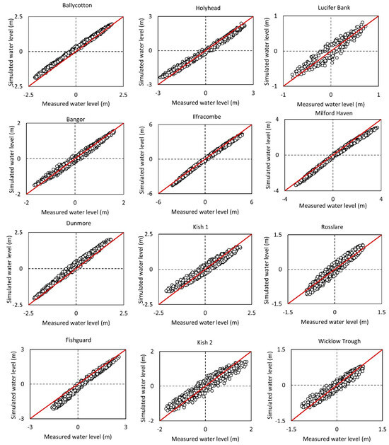
Figure 3.
Comparison between measured and simulated water levels. See Table 1 for location.
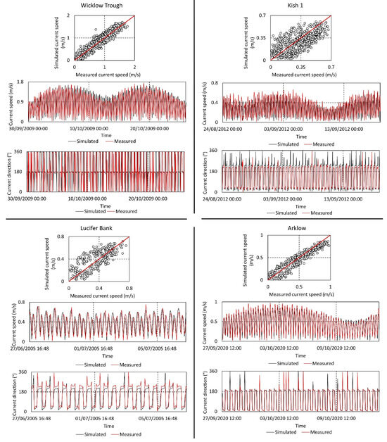
Figure 4.
Calibration profiles of current speed and direction at each of the four ADCP locations (Table 2).
Water levels were re-assessed at eight tide gauges and four ADCPs along the Irish Sea coast and offshore of the south-east coast of Ireland, respectively, over the time periods outlined in Table 1. A strong positive relationship is evident between all measured and simulated water levels (Table 1) where the average correlation coefficient across all locations is 0.99.
Similarly, simulated current speeds and directions were re-assessed against measured data at four locations, including the newly collected Arklow ADCP site. Generally, a strong positive correlation is evident, with the correlation coefficients ranging from 0.84 to 0.95 (Table 2). The notable 30° shift in the major axis of the tidal ellipse on Lucifer Bank shown Coughlan et al. [26] is still evident in this re-analysis. This may be due to the merging of at least two different bathymetry datasets in this location, none of which was captured at the time of the ADCP deployment. Changes in seabed morphology over time have the potential to subsequently alter local hydrodynamics.
2.3.2. ST Modelling Setup
The MIKE 21 sand transport module [82,87] was used to calculate the sediment transport rates of non-cohesive sediment under ‘pure current’, whereby the effects due to wind and wave forcing are not included. The mesh used in the simulation of the sand transport rates is the same as the one that is used to calculate the flow field using the hydrodynamic model described in Section 2.3.1.
A coupled morphological model was generated, whereby the governing equations for flow and sediment transport are merged into a set of equations which are solved simultaneously. Coupling the hydrodynamic and sand transport modules in this way allowed morphological development to be captured by updating the bathymetry for every timestep with the net sedimentation, and it is represented as follows:
where is the bathymetry level at the present timestep, is the bathymetry level at the next timestep, is net sedimentation at the present timestep, and is the timestep. Further details are presented in the MIKE 21 sand transport manual [87]. The key parameter for determination of bed level changes is the rate of bed level change, , at the element cell centres. This parameter is based on the Exner equation, or sediment continuity equation, written as follows:
where is the bed porosity, is the bed level, is the time, is the bed load or total load transport (m2/s) in the direction, is the bed load or total load transport (m2/s) in the direction, and are the horizontal cartesian coordinates, and is the sediment sink or source rate. For a non-equilibrium model such as this, the sediment sink/source term can be written as follows:
where is the normalised no slip level above the bed, is the unit profile function for the sediment concentration, is the settling velocity for the suspended sediment, is the depth-averaged sediment concentration, and is the depth-averaged equilibrium concentration. The bed is updated continuously through a morphological simulation (at every HD timestep, in this case 30 s intervals) based on the estimated bed level change rates. The initial bed thickness of the erodible bed was designated as constant and unlimited throughout the model domain. Slope failure is not included in this morphological model.
The pure current sediment transport theory used in this model was the Engelund and Hansen [89] total-load transport theory. The model by Engelund and Hansen [89] is a total load model that needs user-specified information in order to divide the total load sediment transport into bed load and suspended load transport rates (m2/s) [87]. Transport rates are obtained from the following relations:
whereby and are the user-defined bed load calibration factor and suspended load calibration factor, respectively. Total sediment transport is obtained by the following:
where the Shields parameter is defined as follows:
where is the flow shear stress, is the density of water, is the acceleration due to gravity, s is the relative density of sediment, and is density of sediment. is the Chezy number and is the median grain size. Flow shear stress is divided into form drag and skin friction . The total shear stress is estimated from the local flow velocity and the local Chezy number as follows:
For skin friction the following approximate friction formula is applied:
Sediment density and porosity were defined as constantly 2.65 and 0.40, respectively.
The equilibrium mass concentration () (g/m³) is calculated as the suspended load divided by the water flux and converted from volumetric concentration to mass concentration, as shown in the following equation [87]:
where is the velocity (m/s) and is the water depth.
The following correction is applied to account for the slope effect on the sediment transport rate:
where is the bed level, is the stream-wise (horizontal) coordinate, is the model calibration parameter, is the bed load along streamline , and is the bed load as calculated from sediment transport formula [87].
A varying grain diameter () map was defined for the model domain comprising both surficial and synthetic sediment samples. Surficial sediment samples were collected using either a Day Grab sampler or a Shipek sampler during four MOVE offshore survey campaigns in September 2020 (CV20010), September/October 2020 (CV2036), March 2021 (CV21035), and December 2021 (CV21034). All sediment samples were processed by sieving or laser granulometry. Furthermore, sediment samples containing raw granulometric data were compiled from the Geological Survey of Ireland (GSI). The MOVE and GSI datasets were combined, and statistical analysis to derive values was carried out using the R package ‘geotech’ [90].
Due to limited grain size availability outside our area of interest, the synthetic sand dataset produced by Wilson et al. [72] was utilised. This dataset was clipped to represent the model domain beyond the −70 m contour line extending geographically from Carnsore Point (52.17056°, −6.355278°) to Skerries (53.58389°, −6.101111°). This was to ensure mostly in situ measured grab samples would represent the south-western Irish Sea.
Several artificial values were also placed in the target area using the combined analysis of bathymetry, backscatter, surrounding values, and the EMODnet seabed substrate map. These artificial samples were placed in areas where a significant deficit of measured samples was evident in order to produce the most realistic interpolated dataset when comparing it against coarse seabed substrate maps such as the EMODnet seabed substrate map [91].
2.4. Generation of Seabed Substrate Map Representing the ADCP Deployment Time-Frame
High-quality seabed substrate maps of the Irish Sea have been produced by many organisations such as the Integrated Mapping for Sustainable Development of Ireland’s Marine Resource (INFOMAR) programme [74], the British Geological Survey (BGS) [92], and the European Marine Observation and Data Network (EMODnet) [91]. These seabed classification maps provide a fantastic first indication of the surficial sediment type across the continental shelf sea at a coarse resolution. However, the BGS dataset, for example, Westhead et al. [93], is mainly based on in situ sediment samples that only represent the seabed at one point in time and do not resolve local areas at a fine resolution. Therefore, due to the high mobility of sediment in this area of the Irish Sea [26,30,68] and the lack of existing fine-scale seabed substrate maps, the production of a seabed substrate map on a fine scale over the time period of the ADCP deployment time-frame is imperative to understand the potential particle distribution of sediment in the water column.
During offshore survey CV20010, a multibeam echo sounder (MBES) dataset and two sediment samples, using a day grab sampler, were collected at the site. These datasets were collected on 26 September 2020 and 27 September 2020, respectively. The raw MBES files (.all) were processed for bathymetry and backscatter through Qimera v2.3.1 and FMGT v7.9.5, respectively, whereby the latter is a measure of the strength of the return signal and provides information on the ‘hardness’ of the seabed [94,95,96].
Simultaneously, the sediment samples underwent particle size analysis using the sieve analysis technique. The resulting raw granulometric dataset was processed through the ‘geotech’ R package [90] to derive relevant statistics, such as median grain size () and the grading coefficient. The resulting values are 0.74 mm and 1.01 mm, which according to the Wentworth Scale [97] is coarse sand and very coarse sand, respectively. Upon comparing the general homogenous nature of the backscatter dataset against the composition and location of the two sediment samples, distinguishing two classes of acoustic facies was deemed appropriate for the site. This backscatter dataset was subsequently classified into two classes using the Iso Cluster Unsupervised Classification Tool in ArcGIS v10.8 using a similar method to Evans et al. [98]. The sediment samples were used to ground-truth and further classify the backscatter, ultimately producing a new spatial map of seabed substrate at the site. The processing workflow and end results are provided in Figure 5.
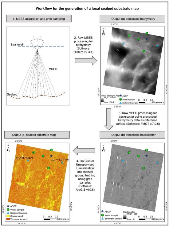
Figure 5.
Workflow diagram of multi-beam echo sounder (MBES) processing and derivation of seabed substrate map over ADCP deployment time period.
2.5. Suspended Sediment Model Validation
In this study, four validation techniques are explored to try to understand the most appropriate method to best validate a 2D suspended sediment transport model. These are as follows:
- Validation of 2D modelled using water sample-based .
- Validation of the flood–ebb characteristics (tidal asymmetry) of (i) 2D modelled suspended load transport and (ii) using ADCP-based datasets.
- ADCP-based validation of 2D modelled using full time series statistics.
- Validation of the 2D modelled peak over a spring–neap cycle using ADCP-based .
The results of these validation techniques are outlined in Section 3.4.
3. Results
3.1. Water Sample-Based
All water samples were tested in the laboratory for total suspended solids (TSS), the results of which are summarised in Table 3. The range of across stations 1 to 4 (Figure 1) is 3.1 mg/L to 10.5 mg/L. These samples were taken between 4 m and 15 m above the seabed at 1 m intervals and within a 300 m radius of the deployed ADCP. They represent approximate slack, peak ebb, and peak flood tidal times. The depth-averaged across this 11 m section of the water column, across all of the four time periods, are consistent, displaying values between 6.7 mg/L and 8.7 mg/L (Figure 6).
Table 3.
Details of water sampling stations including water depth of samples and resulting .
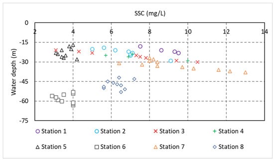
Figure 6.
Scatter plot of all water sample-based samples at stations 1 to 8.
Stations 5 to 8 (Figure 1) are standalone and disassociated from an ADCP deployment. Samples at station 5 and 6 are taken within a one-hour time-frame. Due to the distance of 8 km between stations and the rotary nature of tidal movements in the south Irish Sea around the degenerate amphidromic point located approximately at Courtown [30], both timestamps represent approximately the peak ebb for each location. These samples are taken approximately between 4 m and 15 m above the seabed. The depth-averaged across this 11 m section of the water column is 3.6 mg/L for both stations, whereas the range varies slightly from 3.1 to 4.2 mg/L and 2.9 to 4.0 mg/L for stations 5 and 6, respectively (Figure 6).
Stations 7 and 8 are also taken within a one-hour time-frame and at a separation distance of 9.5 km. They represent approximate peak ebb tide. Similarly to stations 1 to 6, samples at stations 7 and 8 are taken between 4 m and 15 m above the seabed. Station 7 displays higher values compared to station 8. Station 7 ranges from 6.4 mg/L to 13.0 mg/L with a depth-averaged value of 9.3 mg/L, whilst station 8 ranges from 5.6 mg/L to 7.2 mg/L (Figure 6) with a depth-averaged concentration of 6.3 mg/L.
3.2. ADCP Based
A quality check of the processed relative acoustic backscatter identified noise and inconsistencies in bin 1 and bins 27 to 30. As a result, these 5 bins were removed, leaving the processed relative acoustic backscatter recorded in bins 2 to 26, corresponding to 5 m to 29 m above the seabed, as input into the estimation of . Subsequently, approximately 71% of the water column is captured by the processed ADCP relative acoustic backscatter. A strong positive correlation exists between ADCP relative acoustic backscatter and water sample-based , and the correlation coefficient () is 0.89 (Figure 7). The resulting linear regression equation gives a slope of 0.6992 and intercept of −38.848. These slope and intercept values were used in Equation (1) to estimate the time series and spatial distribution of the suspended sediment concentration, which is presented in Figure 8. This equation is specific to this dataset and not applicable to other studies.
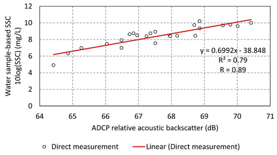
Figure 7.
Calibration of ADCP relative acoustic backscatter data (Beam 4) using the laboratory-analysed .
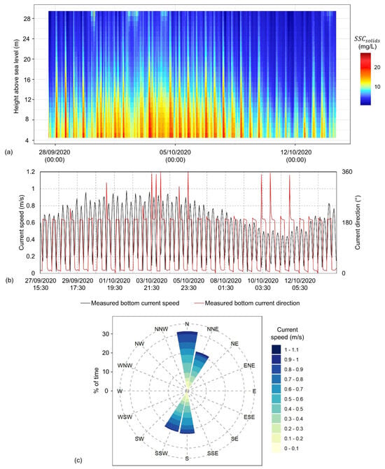
Figure 8.
(a) Beam 4 ADCP-derived spatial time series, (b) bottom current speed and direction recorded by the ADCP, and (c) rose diagram of bottom current speed and direction recorded by the ADCP.
From the ADCP-based spatial time series (Figure 8), the highest fluctuation in concentrations occur between 5 m and 20 m above the seabed. Above this stratum of the water column, significantly reduces, notably varying at a much lesser degree throughout the spring–neap cycle. The maximum and minimum estimated occur at 5 m and 29 m above the seabed on 3 October 2020 at 12:30 (during spring tidal phase) and 11 October 2020 at 15:10 (during neap tidal phase), respectively. The suspended material in the water column most likely comprises substrate material from the seabed, plankton (mainly zooplankton) and other floating microorganisms, and particles. Notably there is a spike in the estimated in the upper bins of the water column at approximately 28 to 29 m above sea level on 30 September 2020, 2 October 2020, 4 October 2020, and 13 October 2020, lasting approximately 11 to 21 h. These four time periods correspond to an increase in significant wave height () and significant wave period () recorded by the two nearest wave buoys of the Irish Marine Data Buoy Observation Network; the M2 buoy located in the Irish Sea at 53.480° N, 5.425° W, and the M5 buoy located in the Celtic Sea at 51.690° N, 6.704° W (Figure 9). With an increase in sea state severity, the depth of penetration of the wave base is increased, causing this noise and unrealistic spikes in the estimated spatial time series.
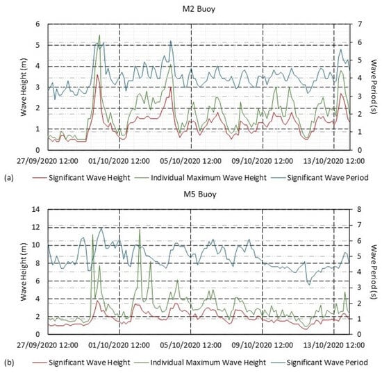
Figure 9.
Wave conditions at (a) M2 Buoy (53.480° N, 5.425° W) and (b) M5 Buoy (51.690° N, 6.704° W) during ADCP deployment.
Figure 5 shows the seabed substrate surrounding the ADCP and water sample locations to be approximately coarse to very coarse sand, with two sediment samples (52.7186° N, 6.0204° W and 52.7201° N, 6.0442° W) in the area displaying a of 1.01 mm and 0.74 mm, respectively. Due to the consistent sandy nature of the seabed substrate at this location and the consistent flood–ebb nature of the tidal flow, the particle distribution of sediment in the water column is expected to be quite consistent. The resuspension of this seabed sediment is highly linked with the tidal cycle, whereby the threshold of motion is more readily exceeded during peak and flood tidal times when relatively higher current speeds exert the highest bed shear stress on the seabed. Some of this sediment may be transported in suspension, given the progressive nature of the tide in a northerly direction (Figure 8), yet some particles may re-settle on the seabed as bed shear stress decreases over slack tide. This settling effect is evident when comparing the recorded water levels and current speeds and directions to the estimated ADCP based spatial time series (Figure 8).
In particular, it is clear from Figure 8 that the suspended sediment is highly linked to the flood and ebb tide. From the current rose produced from the ADCP (Figure 8) and the modelled residual currents it can be seen that a progressive tidal wave is present at this location in the Irish Sea [30], with the flood currents (N to NNE) being more dominant. This is reflected in the suspended sediment profile, whereby a relatively higher amount of sediment is present in the water column during flood tides in comparison to ebbs. Additionally, short drops in concentration along the time series in between the flood and ebb tides correlate with ‘slack’ tide imitating the rectilinear nature of the current at this location. Similarly, the longer increasing and decreasing trend of over this two-week period mimic current patterns over the spring–neap cycle. Where current magnitudes are relatively higher over spring tides (approximately 1st to 6th October 2020) compared to neap tides a higher concentration of is notably present in the water column. As the average current speeds over spring tides is higher than neaps, it is more likely for a higher percentage of sediment to remain in the water column over the flood–ebb cycle rather than completely settle to the seafloor compared to neap currents.
3.3. Comparison Between ADCP-Based and Water Sample-Based
In order to quality check the accuracy of the ADCP estimated , ADCP-based values corresponding directly to the timestamp and water depth of the water sample-based were extracted and compared. A strong positive linear relationship () exists between the measured and estimated values (Figure 10). Figure 10 shows that the best correlation exists within the value range of 7 mg/L to 9 mg/L. The values below this range are slightly overestimated by the ADCP-based , and the values above this range are slightly underestimated. Increasing the number of water samples over the ADCP deployment time-frame may further improve the correlation between ADCP estimated and water sample-based in future studies. Regardless, this strong relationship ultimately provides a high level of confidence for the ADCP-derived time series. This shows that are accurately estimated by the ADCP’s acoustic backscatter.
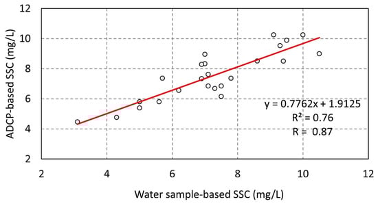
Figure 10.
Linear regression between water sample-based samples and ADCP-derived .
3.4. Suspended Sediment Model Validation
In this section, four validation techniques are explored to try to understand the most appropriate method to best validate a 2D suspended sediment transport model.
3.4.1. Technique 1: Validation of 2D Modelled Using Water Sample-Based
Technique 1 involves the comparison between modelled and directly measured collected via water sampling at four stations not associated with ADCP deployments. These include stations 5 to 8, the details of which are provided in Table 3. Each of these samples were taken at approximately peak flood or peak ebb tidal times. In order to validate the model using these samples, the modelled peak at these corresponding timestamps, and the modelled peak seven days before and after the sampling date, representing a full spring–neap tidal cycle, were extracted and subsequently plotted in Figure 11.
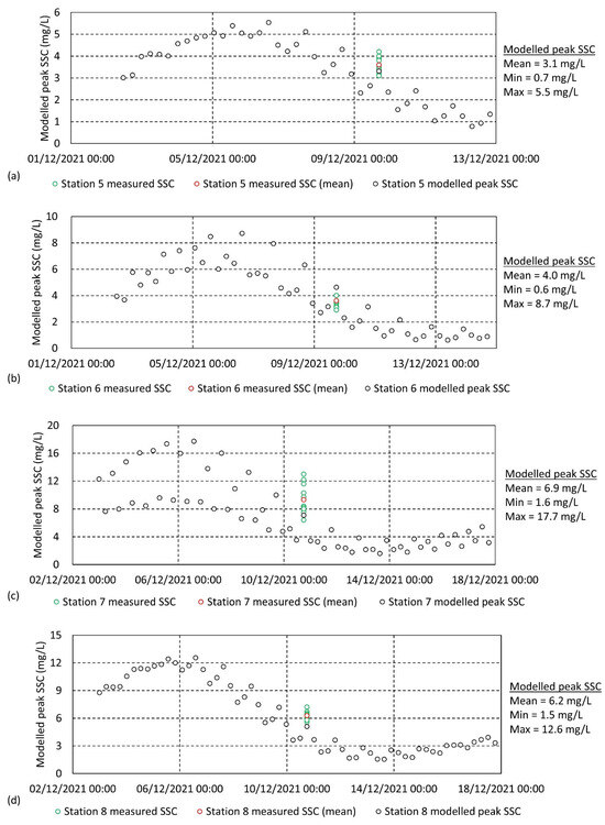
Figure 11.
Comparison of 2D modelled peak against measured samples at four sampling stations not associated with ADCP deployments: (a) Station 5, (b) Station 6, (c) Station 7, and (d) Station 8. Sampling station locations are presented in Figure 1.
Notably, each location displays a strong relationship between directly measured and modelled . Figure 11a displays results at station 5. Modelled values at the time of sampling and the modelled peak mean concentration over the spring–neap cycle are 3.3 mg/L and 3.1 mg/L, respectively. These values show a very good agreement with the mean measured of 3.6 mg/L.
Similarly, output at the time of direct sampling at station 6 is 4.6 mg/L, where the overall modelled peak mean over the spring–neap cycle is 4.0 mg/L. These compare well with mean measured , 3.6 mg/L.
Figure 11c displays results at station 7. Direct sampling results range from 6.4 mg/L to 13.0 mg/L, with an average of 9.3 mg/L. The modelled output at this timestamp, 7.1 mg/L, and the modelled peak mean over the spring–neap cycle, 6.9 mg/L, compare well with these values.
Furthermore, Figure 11d displays very good agreement between mean measured , 6.3 mg/L, and modelled values, whereby modelled at that timestamp is 5.1 mg/L and the modelled peak mean over the spring–neap cycle is 6.2 mg/L.
3.4.2. Technique 2: Validation of the Flood–Ebb Characteristics (Tidal Asymmetry) of (i) 2D Modelled Suspended Load Transport and (ii) , Using ADCP-Based Datasets
Validation of Tidal Asymmetry in 2D Modelled Suspended Load Transport
As outlined in Section 3.2, measured currents at the site exhibit a flood-dominant tidal current in a north to north–north-easterly direction. Modelled residual tidal current and residual suspended load transport agree with the nature of this tidal asymmetry (Figure 12), ultimately providing a high degree of confidence for the directional component of modelled suspended sediment transport at this location.
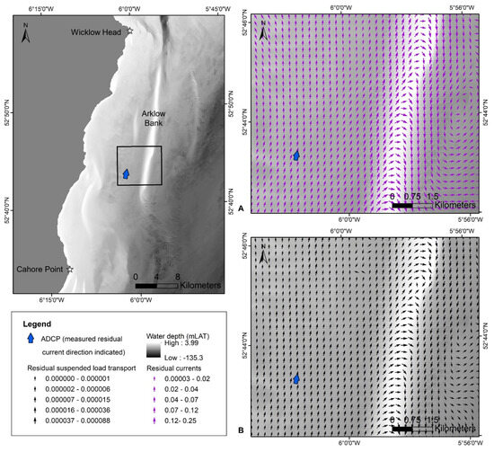
Figure 12.
(A) Modelled residual currents. (B) Modelled residual suspended sediment transport.
Validation of Tidal Asymmetry in 2D Modelled
In parallel, the ADCP-based spatial time series can be used as a calibration/validation technique for the relative magnitude of modelled in the water column over a flood–ebb tidal cycle. For example, the impact of the progressive tidal wave on suspended sediment transport in this local environment is clear when analysing the rose diagram (Figure 13) of estimated bottom-water, mid-water, surface-water, and depth-averaged ADCP-based alongside measured current directions. All four time series (Figure 13) display a higher concentration of in the water column for a higher percentage of time during the flood tide compared to the ebb tide. This is a direct consequence of the flood-dominance nature of the tide. The rose diagram of modelled alongside modelled current directions show a very good agreement with this asymmetrical tide–SSC relationship, whereby a higher concentration of is present in the water column also over the flood tide (N—NNE) in comparison to the ebb tide (S—SSW) (Figure 13).
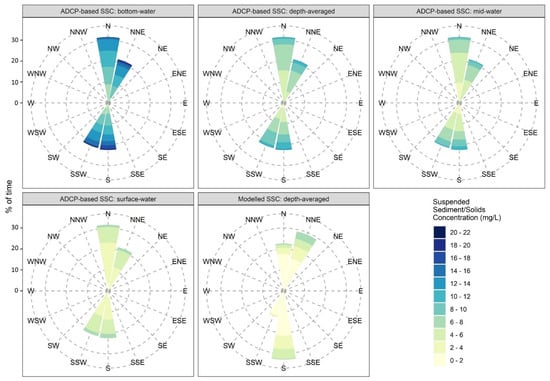
Figure 13.
Roses of bottom-water, mid-water, surface-water, and depth-averaged ADCP-based suspended solids concentration with measured current directions from 27 September 2020 at 15:00 to 14 October 2020 at 09:00. Modelled depth-averaged suspended sediment concentration with modelled current directions over the same time period.
3.4.3. Technique 3: ADCP-Based Validation of 2D Modelled Using Full Time Series Statistics
Full time series statistics are generated for bottom-water, mid-water and surface-water ADCP-based and are compared against modelled over the same time period. Results are displayed in Table 4 where variation between modelled and estimated datasets is evident. These will be discussed further in Section 4.2.
Table 4.
Minimum, maximum, and mean ADCP-based at bottom-water, mid-water, surface water, and depth-averaged, and statistics from full dataset of modelled .
3.4.4. Technique 4: Validation of the 2D Modelled Peak over a Spring–Neap Cycle Using ADCP-Based
Modelled peak values (maximum concentration over each flood and ebb tide) from 27 September 2020 at 15:00 to 14 October 2020 at 09:00 were extracted, corresponding to the time-frame of the ADCP deployment. Simultaneously, three time series were generated from the ADCP-based spatial time series by calculating the minimum, mean (depth-averaged), and maximum values across all ADCP bins for all timesteps. Subsequently, the minimum, mean, and maximum ADCP-based , corresponding to the same timestep of the modelled peak values, were extracted and compared. The resulting comparison is presented in Figure 14.
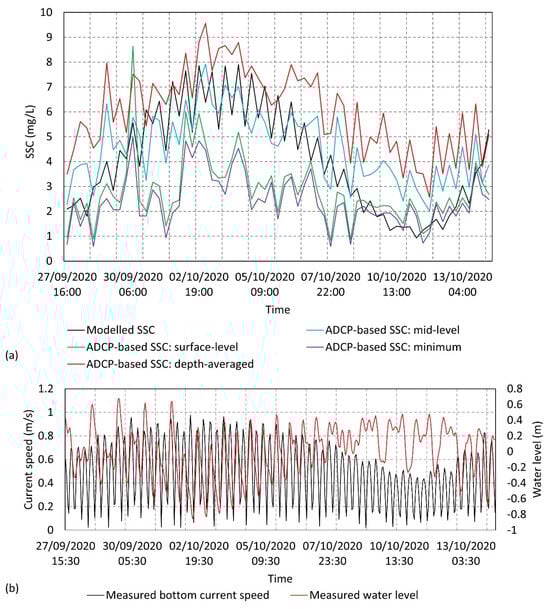
Figure 14.
(a) Comparative time series plot of 2D modelled suspended sediment concentration against ADCP-derived suspended solids concentration and (b) water level and bottom current speed recorded by the ADCP.
An overall increase and decrease in modelled peak is evident over the spring and neap tidal phases, respectively. This same trend is reflected both in the full spatial ADCP-based time series (Figure 8) and in the depth-averaged profile (Figure 14). The modelled output has a better agreement with depth-averaged ADCP-based over spring tides yet agrees better with the minimum profile over the neap tidal phase (Figure 14). Nevertheless, the peak modelled lies between the minimum and depth-averaged ADCP-based profiles. A strong positive relationship exists between the depth-averaged and modelled peak , where is 0.82 (Figure 15a). Additionally, a moderate positive relationship is present between the minimum and modelled peak , where is 0.58 (Figure 15b). Overall, a good agreement is evident.
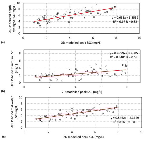
Figure 15.
Correlation between (a) 2D modelled peak and ADCP-based depth-averaged , (b) 2D modelled peak and ADCP-based minimum , and (c) 2D modelled peak and ADCP-based mid-water .
These modelled peak SSC values are further compared to the ADCP-based bottom-water, mid-water, and surface-water values (Figure 14). The modelled dataset shows a very good agreement with mid-water ADCP-based over the full spring–neap time-frame. Where correlation drops slightly over the neap tidal phase from approximately 9 October to 13 October 2020, the modelled output aligns very well with surface-water estimations. The relationship between these modelled values and the mid-water ADCP based is strong positive, where is 0.81 (Figure 15c). It is noted in Figure 14 that the surface-water contour unrealistically surpasses or becomes close to the mid-water contour during the periods of relatively higher sea-state, as outlined in Section 3.2. This is due to larger surface waves extending deeper into the water column, ultimately causing higher levels of noise in deeper bins.
4. Discussion
4.1. Evaluation of the Ability to Estimate from ADCP Relative Acoustic Backscatter in a Shallow Shelf Sea Environment
To convert echo intensity recorded by the ADCP to a clean, processed relative acoustic backscatter dataset, a literature review was first carried out to select the most suitable equations and to establish a robust workflow. The ultimate equations adopted in this study account for spreading losses in both the far and near fields [67,78] and transmission losses due to both the absorption of seawater [79] and the attenuation of acoustic energy by suspended particles [80]. Comparing results at various stages of the processing workflow, provided in Section 2.2, to previous studies yielded very good correlations. The absorption coefficient due to water ) calculated in this study (0.087 dB/m) shows good agreement with that presented in Mullison [53] (0.068 dB/m). Similarly, Baranya and Józsa’s [51] concentration value of 0.0005 dB/m for 1 mg/L correlates very well with the concentration value of 0.00048 dB/m calculated in this study. Additionally, when plotting the reverberation level () (Equation (5)), the when corrected for spreading losses (), and the when corrected for spreading losses and fluid and suspended particle losses () on the same line chart, the relative change in their line slope gradients is highly similar to that presented in Landers [55].
A high degree of confidence is also revealed in the estimation of ADCP-based , whereby a strong positive correlation exists between (i) ADCP relative acoustic backscatter and water sample-based and (ii) measured and estimated values, with a correlation coefficient of 0.89 and 0.87, respectively. The magnitude of these correlation coefficients are analogous to results in previous studies [51,64,67,75].
As previously discussed, single-frequency systems cannot differentiate between the change in concentration of suspended material in the water column and the change in particle size distribution (PSD) of the suspended sediment [59]. The magnitude of error varies depending on the instrument frequency and the amount of change in PSD [59]. This error could be considered negligible in this case when considering the following three variables; (i) the successful production of an estimated seabed substrate map at the study site for the beginning of the ADCP deployment, revealing a relatively consistent course sandy seabed (Section 2.4 and Section 3.2); (ii) combining (i) with a consistent flood–ebb semi-diurnal tidal system that is absent of flow related phenomena that could suddenly change the background PSD of suspended particles, e.g., muddy storm run-off in coastal waters, implies a relatively consistent PSD in the suspended sediment load; and (iii) the relatively low frequency of the ADCP (300 kHz) means a lower sensitivity to very fine particles in comparison to higher frequency instruments, thus reducing the potential for error.
The ability to produce an estimated spatial time series of using processed relative acoustic backscatter has therefore proven to be successful in this study. The processed acoustic dataset provides excellent coverage of the water column at the ADCP deployment site, capturing approximately 71% of the water column over a full spring–neap tidal cycle. The resulting estimated spatial time series in combination with ADCP-based hydrodynamic parameters provides invaluable information in terms of dynamics in this complex hydrodynamic system. The impacts of the prominent tidal asymmetry phenomenon on sediment dynamics could be observed over both the flood–ebb and spring–neap tidal cycles. These ADCP-based datasets provide a more wholistic understanding of the interaction of these phenomena than sole water-sampling or OBS deployment.
4.2. Evaluation of Model Validation Techniques
The suspended sediment transport component of the 2D model is deemed successfully validated at multiple locations off the east coast of Ireland to a relatively high accuracy given the underlying assumptions of the model using tested validation techniques.
Specifically, three out of four assessed validation techniques are deemed useful in developing the most accurate 2D suspended sediment transport model. In particular, combined use of technique 1, 2, and 4 provide (i) validation at one timestamp, (ii) validation of tidal asymmetry (flood–ebb characteristics) averaged over a full spring–neap tidal phase, and (iii) validation of the dissected trends and magnitudes across a full spring–neap cycle, or the length of an ADCP deployment.
Technique 1 displays very good validation results and proves highly useful as extra validation points across a model domain. Depending on the size of the numerical model in question or the area of interest within a large model domain, water sampling used in this way may be useful for providing supplementary validation points to ADCP deployments. This technique is recommended to combine with techniques 2 and 4.
Technique 2 provides a very good method to validate the characteristics of suspended load transport and directly linked with tidal asymmetry. This method is best combined with techniques 1 and 4.
Technique 3 is deemed unsuitable as a validation technique for 2D modelled . The results highlight variations between modelled and ADCP-estimated . The potential reasons for these variations include the following:
- (i)
- The ADCP-based time series, representing approximately 71% of the water column, is estimated for suspended solids concentration. This comprises mainly sediment but may also contain floating micro-organisms and other particles. Therefore, this estimated dataset may naturally display a higher concentration of suspended solids compared to 2D modelled suspended sediment.
- (ii)
- The ADCP-based time series could not capture the bottom 5 m and the top 5 m of the water column. The bottom 5 m of the water column generally contains the highest concentrations of suspended sediment; these concentrations generally decrease as you progress toward the surface. The absence of these strata may skew full time series general (mean/minimum/maximum) statistics.
- (iii)
- Similarly to other studies [11], at every slack water over this spring–neap time-frame the 2D modelled drops down to approximately 0. Realistically, this does not naturally occur in this continental shelf environment, showing the limitation of this depth-integrated approach for suspended sediment transport modelling. This 2D modelled time series does not fully capture the full complexity of the natural environment, therefore, it may not be practical to compare SSC magnitude like for like through these general statistics.
The three points outlined above suggest that a 3D model may be more useful in terms of trying to capture the full complexity of hydrodynamics and sediment transport over the full water column. However, this is not always practically feasible when considering computational time, model resolution, and project budget. Therefore, the best calibration/validation technique to provide the most accurate 2D suspended sediment transport model is to compare the peak modelled against corresponding peak ADCP-based . This is explored as technique number 4.
Technique 4, whereby 2D modelled is compared against minimum, depth-averaged, mid-water, and surface-water ADCP-based profiles over a spring–neap cycle, provides the best validation technique for this location. Analysing the 2D modelled peak in this way allows the disintegration of general data trends and magnitude ranges over a full spring–neap cycle. Additionally, although the 2D modelled peak lies within the minimum and depth-averaged ADCP-based thresholds and show moderate to strong positive relationships, a comparison against the mid-water and surface-water ADCP-based proves more useful at this site. In this case, the modelled peak SSC correlates very well with mid-water ADCP estimates. Contrastingly, it is found that using the bottom-water ADCP-based time series as a calibration/validation dataset would be inappropriate as this stratum contains much higher concentrations over a relatively small proportion of the water column and therefore is not representative of a depth-averaged water column. As a result, it is not recommended to compare like for like against depth-averaged modelled . A similar view has been determined for the maximum ADCP-based profile.
Although technique 1 is considered highly useful, the ability to dissect the time series across a full spring–neap cycle using ADCP-based methods in techniques 2 and 4 is invaluable. Depending on the size of the sediment transport model developed or the area of interest within a numerical model, multiple ADCP deployments and/or water sample stations will enhance model validation accuracy. These ADCP-based techniques are considered very cost-effective as the deployment of acoustic instruments are already necessary in order to provide validation information for hydrodynamic models, and in some cases, wave models [99]. An additional water sampling campaign over the ADCP deployment period, both in the proximity of the deployed ADCP and in other areas of the model domain, could be of huge benefit and add a wealth of knowledge to the site area. These three techniques can ultimately be combined with bed load validation techniques, for example, bed level changes using bathymetry datasets [12,38], to provide an increasingly accurate sediment transport model in tidally dominated environments.
4.3. Potential Improvements/Future Work
Potential improvements in methods and areas for future investigation have been identified in two distinct subject areas: (i) the estimation of ADCP-based and (ii) the validation and calibration of numerical modelling work. Details of these are outlined below.
- (i)
- The estimation of ADCP-based :
- a.
- Increasing the number of water samples over the ADCP deployment time-frame may further improve correlation between ADCP relative acoustic backscatter and water sample-based
- b.
- Improvements in the existing ADCP deployment setup. This could involve the use of an acoustic release to allow for survey vessel instrumentation to obtain water samples closer to the deployed ADCP. Practically, however, even with the use of an acoustic release, the ability to improve proximity to the ADCP may not be feasible given the relatively high surface current speeds in the south-western Irish Sea and other offshore environments during peak flood and ebb times due to vessel drift. In this case, vessel specifications such as dynamic positioning and operability statistics could be considered more specifically for this purpose if project budget allows.
- c.
- Investigating other techniques such as the use of a hull-mounted or downward-looking ADCPs [67], multi-frequency ADCPs, and other sediment transport measurement-specific instruments such as Aquascat sediment concentration profilers could also be investigated for the purpose of numerical model validation. For example, where a change in PSD is expected, the use of dual frequency ADCPs is expected to provide a high accuracy of results.
- d.
- The methods and techniques developed in this study could be directly applied to other tidally dominated continental shelf seas on a global scale. However, the south-western Irish Sea is dominated by sand to gravelly sand [30] and exhibits a semi-diurnal tidal cycle [30]. Other offshore environments earmarked for ORE developments diversify from these hydrodynamic and sediment characteristics. Therefore, the estimation of from ADCP acoustic backscatter could be further tested in other continental shelf seas around the world.
- (ii)
- Calibration and validation of numerical modelling work:
- a.
- As outlined in Section 4.2, techniques 1, 3, and 4 prove very good validation methods for 2D numerical modelling work. However, technique 2 highlights the limitation of the depth-integrated modelling approach to capture the full dynamics of the natural sediment transport regime. In many coastal and offshore modelling studies the underlying assumptions of a 2D modelling approach is accepted and is commonly the most feasible approach in comparison to other numerical modelling techniques such as 3D and SPH. In making this decision, many variables are commonly considered including model domain size, spatial and temporal resolution requirements, computational power, and project scope, timeline, and budget, and also site-specific environmental variables such as water stratification, the consistency of the vertical current profile, and the complexity of regional scale hydrodynamics and morphodynamics. On a small to medium scale, 3D sediment transport models in coastal and offshore environments are becoming increasingly more feasible. In this case, the direct application of these newly tested validation techniques to a 3D model could be investigated. Additionally, the full 71% coverage of the ADCP-based spatial time series has high potential for additional validation of various layers of the modelled water column. By performing this the limitations of the depth-integrated 2D modelling approach of fully characterising suspended load transport could be compared to a 3D modelling approach.
5. Conclusions
The main conclusions that have emerged from this research are summarised as follows:
- (1)
- The estimation of from ADCP acoustic backscatter based on sonar equations has proven successful in a tidally dominated shallow shelf sea setting. A strong positive correlation is evident both between water sample-based and ADCP acoustic backscatter (), and water sample-based and ADCP-estimated (). These relationships provide a high degree of confidence in the accuracy of the ADCP-estimated spatial time series.
- (2)
- The suspended sediment transport component of the 2D model is deemed successfully validated using three of the four tested model validation techniques. The successful model validation techniques include the following:
- Validation of 2D modelled using water sample-based .
- Validation of the flood–ebb characteristics (tidal asymmetry) of (i) 2D modelled suspended load transport and (ii) using ADCP-based datasets.
- Validation of the 2D modelled peak over a spring–neap cycle using ADCP-based .
These techniques have produced highly acceptable results for this area of interest and have a high potential to be applicable in other locations. - (3)
- The development of a local seabed substrate map using ground-truthed MBES backscatter proved to be a useful technique to provide crucial information on site-specific seabed sediment characteristics over the ADCP deployment time-frame.
- (4)
- The ADCP-based spatial time series has the potential to provide additional validation of the vertical layers in a 3D model. The application of the ADCP-based techniques in this way could reveal how or if a 3D model could overcome the limitations of a depth-integrated 2D modelling approach in fully characterising the natural variability of in a tidally dominated shallow shelf sea setting. Further investigation is recommended.
- (5)
- The multi-disciplinary method of collecting in situ metocean and sediment dynamic data via acoustic instruments (ADCPs) is a cost-effective procedure for future ORE development projects and other engineering and scientific works.
Author Contributions
Conceptualization, S.C.; Formal analysis, S.C.; Investigation, S.C. and M.C.; Writing—original draft, S.C.; Writing—review & editing, S.C., M.O. and J.M.; Supervision, M.O., M.C. and J.M. All authors have read and agreed to the published version of the manuscript.
Funding
S.C. is funded by the Irish Research Council (IRC) through grant EBPPG/2019/158 (Employment-Based Postgraduate Programme Scholarship). M.C. is funded under an Irish Research Council Enterprise Partnership Scheme Postdoctoral Fellowship (EPSPD/2020/109) and in part by a research grant from Science Foundation Ireland (SFI) under Grant Number 13/RC/2092, with support from Gavin and Doherty Geosolutions Ltd. and the Geological Survey of Ireland (GSI). This project benefitted from funded industry–academic collaboration involving Gavin and Doherty Geosolutions, University College Dublin (iCRAG), and University College Cork (MaREI), supported by the Marine Institute under the Marine Research Programme 2014–2020 (Grant-Aid Agreement No. IND/18/18). Ship time on the RV Celtic Voyager was funded by the Marine Institute through the 2020–2021 ship-time programme under the National Marine Research and Innovation Strategy 2017–2021.
Data Availability Statement
The original contributions presented in this study are included in the article. Further inquiries can be directed to the corresponding author.
Acknowledgments
The authors would gratefully like to acknowledge the Mobility of Sediment Waves and Sand Banks in the Irish Sea (MOVE) (CV20010, CV20036, CV21034, and CV21035) shipboard crew and scientists, and onshore Marine Institute and INFOMAR support personnel for assistance with data acquisition. The authors are appreciative for access to the seabed sediment sample data and would like to acknowledge colleagues collecting and preparing these data through the projects and surveys mentioned. The authors wish to thank Xavier Monteys and Charise McKeon (both GSI) for aiding with the INFOMAR dataset.
Conflicts of Interest
The authors declare no conflict of interest.
References
- Aijaz, S.; Driscoll, A.; Sayce, A.; Kaegaard, K.; Klabbers, M.; Misra, S. Fine sediment transport modelling for design of port facilities. In Coasts and Ports 2013: 21st Australasian Coastal and Ocean Engineering Conference and the 14th Australasian Port and Harbour Conference; Engineers Australia: Barton, Australia, 2013. [Google Scholar]
- de Schipper, M.A.; Ludka, B.C.; Raubenheimer, B.; Luijendijk, A.P.; Schlacher, T.A. Beach nourishment has complex implications for the future of sandy shores. Nat. Rev. Earth Environ. 2021, 2, 70–84. [Google Scholar] [CrossRef]
- Karambas, T.V.; Samaras, A.G. Soft shore protection methods: The use of advanced numerical models in the evaluation of beach nourishment. Ocean Eng. 2014, 92, 129–136. [Google Scholar] [CrossRef]
- Benassai, G. Introduction to Coastal Dynamics and Shoreline Protection; Wit Press: Southampton, UK, 2006. [Google Scholar]
- Creech, C.T.; Amorim, R.S.; Castanon, A.N.A.O.; Gibson, S.A.; Veatch, W.C.; Lauth, T.J. A planning framework for Improving reliability of inland navigation on the Madeira River in Brazil. In Proceedings of the PIANC-World Congress, Panama City, Panama, 7–11 May 2018; pp. 1–20. [Google Scholar]
- Duman, M.; Kucuksezgin, F.; Atalar, M.; Akcali, B. Geochemistry of the northern Cyprus (NE Mediterranean) shelf sediments: Implications for anthropogenic and lithogenic impact. Mar. Pollut. Bull. 2012, 64, 2245–2250. [Google Scholar] [CrossRef]
- Mcbreen, F.; Wilson, J.G.; Mackie, A.S.Y.; Aonghusa, C.N. Seabed mapping in the southern Irish Sea: Predicting benthic biological communities based on sediment characteristics. Hydrobiologia 2008, 606, 93–103. [Google Scholar] [CrossRef]
- Jones, C.; Magalen, J.; Roberts, J. Wave Energy Converter (WEC) Array Effects on Wave, Current, and Sediment Circulation: Monteray Bay, CA; Sandia National Laboratories: Santa Cruz, CA, USA; Albuquerque, NM, USA, 2014. [Google Scholar]
- Abanades, J.; Greaves, D.; Iglesias, G. Wave farm impact on the beach profile: A case study. Coast. Eng. 2014, 86, 36–44. [Google Scholar] [CrossRef]
- Neill, S.P.; Robins, P.E.; Fairley, I. The Impact of Marine Renewable Energy Extraction on Sediment Dynamics. In Marine Renewable Energy: Resource Characterization and Physical Effects; Yang, Z., Copping, A., Eds.; Springer International Publishing: Berlin/Heidelberg, Germany, 2017; pp. 279–304. [Google Scholar] [CrossRef]
- Robins, P.E.; Neill, S.P.; Lewis, M.J. Impact of tidal-stream arrays in relation to the natural variability of sedimentary processes. Renew. Energy 2014, 72, 311–321. [Google Scholar] [CrossRef]
- Auguste, C.; Nader, J.R.; Marsh, P.; Penesis, I.; Cossu, R. Modelling the influence of Tidal Energy Converters on sediment dynamics in Banks Strait, Tasmania. Renew. Energy 2022, 188, 1105–1119. [Google Scholar] [CrossRef]
- Ivanov, E.; Capet, A.; De Borger, E.; Degraer, S.; Delhez, E.J.; Soetaert, K.; Vanaverbeke, J.; Grégoire, M. Offshore Wind Farm Footprint on Organic and Mineral Particle Flux to the Bottom. Front Mar Sci. 2021, 8, 631799. [Google Scholar] [CrossRef]
- Whitehouse, R.J.S.; Harris, J.M.; Sutherland, J.; Rees, J. The nature of scour development and scour protection at offshore windfarm foundations. Mar. Pollut. Bull. 2011, 62, 73–88. [Google Scholar] [CrossRef]
- IEA. Net Zero by 2050. A Roadmap for the Global Energy Sector. Revised version, October 2021 (4th Revision); International Energy Agency: Paris, France, 2021. [Google Scholar]
- IEA. World Energy Outlook 2022. Revised Version, November 2022. Available online: https://iea.blob.core.windows.net/assets/830fe099-5530-48f2-a7c1-11f35d510983/WorldEnergyOutlook2022.pdf (accessed on 1 September 2023).
- Rivier, A.; Bennis, A.-C.; Pinon, G.; Magar, V.; Gross, M. Parameterization of wind turbine impacts on hydrodynamics and sediment transport. Ocean Dyn. 2016, 66, 1285–1299. [Google Scholar] [CrossRef]
- Baeye, M.; Fettweis, M. In situ observations of suspended particulate matter plumes at an offshore wind farm, southern North Sea. Geo-Mar. Lett. 2015, 35, 247–255. [Google Scholar] [CrossRef]
- Fairley, I.; Masters, I.; Karunarathna, H. The cumulative impact of tidal stream turbine arrays on sediment transport in the Pentland Firth. Renew. Energy 2015, 80, 755–769. [Google Scholar] [CrossRef]
- Harris, J.M.; Whitehouse, R.J.S.; Sutherland, J. Marine scour and offshore wind-Lessons learnt and future challenges. In Proceedings of the International Conference on Offshore Mechanics and Arctic Engineering-OMAE, 2011, Rotterdam, The Netherlands, 19–24 June 2011; pp. 849–858. [Google Scholar] [CrossRef]
- Lind, R.A.; Whitehouse, R.J.S. Understanding and Assessing Scour Development at Offshore Structures. J. Oilfield Technol. 2012, 5, 63–67. [Google Scholar]
- van Berkel, J.; Burchard, H.; Christensen, A.; Mortensen, L.O.; Petersen, O.S.; Thomsen, F. The Effects of Offshore Wind Farms on Hydrodynamics and Implications for Fishes. Oceanography 2020, 33, 108–117. [Google Scholar] [CrossRef]
- Clark, S.; Schroeder, F.; Baschek, B. The Influence of Large Offshore Wind Farms on the North Sea and Baltic Sea–A Comprehensive Literature Review (Report No. HZG Report 2014-6); Helmholtz-Zentrum Geesthacht, Zentrum für Material-und Küstenforschung: Geesthacht, Germany, 2014. [Google Scholar]
- Bat, L.; Sezgin, M.; Sahin, F. Impacts of OWF installations on fisheries: A Literature Review. J. Coast. Life Med. 2013, 1, 241–252. [Google Scholar] [CrossRef]
- Onea, F.; Rusu, L.; Carp, G.B.; Rusu, E. Wave farms impact on the coastal processes—A case study area in the portuguese nearshore. J. Mar. Sci. Eng. 2021, 9, 262. [Google Scholar] [CrossRef]
- Coughlan, M.; Guerrini, M.; Creane, S.; O’Shea, M.; Ward, S.L.; Van Landeghem, K.J.; Murphy, J.; Doherty, P. A new seabed mobility index for the Irish Sea: Modelling seabed shear stress and classifying sediment mobilisation to help predict erosion, deposition, and sediment distribution. Cont. Shelf Res. 2021, 229, 104574. [Google Scholar] [CrossRef]
- Roetert, T.; Raaijmakers, T.; Borsje, B. Cable route optimization for offshore wind farms in morphodynamic areas. In Proceedings of the 27th International Offshore and Polar Engineering Conference, San Francisco, CA, USA, 25–30 June 2017; pp. 595–606. [Google Scholar]
- Harris, J.M.; Whitehouse, R.J.S. Scour management—A risk based approach. In Proceedings of the 6th International Conference of Scour and Erosion (ICSE-6), Paris, France, 27–31 August 2012. [Google Scholar]
- van der Tempel, J.; Zaaijer, M.B.; Subroto, H. The effects of Scour on the design of offshore wind turbines. In Proceedings of the 3rd International Conference on Marine Renewable Energy, Blyth, UK, 7–9 July 2004; pp. 27–35. [Google Scholar]
- Creane, S.; O’Shea, M.; Coughlan, M.; Murphy, J. The Irish Sea bed load parting zone: Is it a mid-sea hydrodynamic phenomenon or a geological theoretical concept? Estuar. Coast. Shelf Sci. 2021, 263, 107651. [Google Scholar] [CrossRef]
- Li, M.Z.; Hannah, C.G.; Perrie, W.A.; Tang, C.C.L.; Prescott, R.H.; Greenberg, D.A. Modelling seabed shear stress, sediment mobility, and sediment transport in the bay of fundy. Can. J. Earth Sci. 2015, 52, 757–775. [Google Scholar] [CrossRef]
- Brown, J.M.; Davies, A.G. Methods for medium-term prediction of the net sediment transport by waves and currents in complex coastal regions. Cont. Shelf Res. 2009, 29, 1502–1514. [Google Scholar] [CrossRef]
- Rivier, A.; Bennis, A.C.; Pinon, G.; Gross, M.; Magar, V. Regional numerical modelling of offshore monopile wind turbine impacts on hydrodynamics and sediment transport. In Proceedings of the Renewable Energies Offshor-1st International Conference on Renewable Energies Offshore, RENEW 2014, Lisbon, Portugal, 23–25 November 2014; pp. 807–814. [Google Scholar] [CrossRef]
- Couldrey, A.J.; Benson, T.; Knaapen, M.A.F.; Marten, K.V.; Whitehouse, R.J.S. Morphological evolution of a barchan dune migrating past an offshore wind farm foundation. Earth Surf. Process Landf. 2020, 45, 2884–2896. [Google Scholar] [CrossRef]
- Neill, S.P.; Couch, S.J. Impact of Tidal Energy Converter (TEC) Array Operation on Sediment Dynamics. In Proceedings of the 9th European Wave and Tidal Energy Conference (EWTEC), Southampton, UK, 5–9 September 2011. [Google Scholar]
- Borsje, B.W.; Roos, P.C.; Kranenburg, W.M.; Hulscher, S.J.M.H. Modeling tidal sand wave formation in a numerical shallow water model: The role of turbulence formulation. Cont. Shelf Res. 2013, 60, 17–27. [Google Scholar] [CrossRef]
- Krabbendam, J.; Nnafie, A.; de Swart, H.; Borsje, B.; Perk, L. Modelling the past and future evolution of tidal sand waves. J. Mar. Sci. Eng. 2021, 9, 1071. [Google Scholar] [CrossRef]
- Leenders, S.; Damveld, J.H.; Schouten, J.; Hoekstra, R.; Roetert, T.J.; Borsje, B.W. Numerical modelling of the migration direction of tidal sand waves over sand banks. Coast. Eng. 2021, 163, 103790. [Google Scholar] [CrossRef]
- Tran-Duc, T.; Phan-Thien, N.; Khoo, B.C. A smoothed particle hydrodynamics (SPH) study of sediment dispersion on the seafloor. Phys. Fluids 2017, 29, 83302. [Google Scholar] [CrossRef]
- Fairley, I.; Masters, I.; Karunarathna, H. Numerical modelling of storm and surge events on offshore sandbanks. Mar. Geol. 2016, 371, 106–119. [Google Scholar] [CrossRef]
- Auguste, C.; Marsh, P.; Nader, J.R.; Penesis, I.; Cossu, R. Modelling morphological changes and migration of large sand waves in a very energetic tidal environment: Banks Strait, Australia. Energies 2021, 14, 3943. [Google Scholar] [CrossRef]
- Ashall, L.M.; Mulligan, R.P.; Law, B.A. Variability in suspended sediment concentration in the Minas Basin, Bay of Fundy, and implications for changes due to tidal power extraction. Coast. Eng. 2016, 107, 102–115. [Google Scholar] [CrossRef]
- Ulses, C.; Estournel, C.; de Madron, X.D.; Palanques, A. Suspended sediment transport in the Gulf of Lions (NW Mediterranean): Impact of extreme storms and floods. Cont. Shelf Res. 2008, 28, 2048–2070. [Google Scholar] [CrossRef]
- Guillén, J.; Palanques, A.; Puig, P.; de Madron, X.D.; Nyffeler, F. Field calibration of optical sensors for measuring suspended sediment concentration in the western Mediterranean. Sci. Mar. 2000, 64, 427–435. [Google Scholar] [CrossRef]
- Downing, J. Twenty-five years with OBS sensors: The good, the bad, and the ugly. Cont. Shelf Res. 2006, 26, 2299–2318. [Google Scholar] [CrossRef]
- Boss, E.; Sherwood, C.R.; Hill, P.; Milligan, T. Advantages and limitations to the use of optical measurements to study sediment properties. Appl. Sci. 2018, 8, 2692. [Google Scholar] [CrossRef]
- Kerr, A.; Cowling, M.J.; Beveridge, C.M.; Smith, M.J.; Parr, A.C.; Head, R.M.; Davenport, J.; Hodgkiess, T. The early stages of marie biofouling and its effect on two types of optical sensors. Environ. Int. 1998, 24, 331–343. [Google Scholar] [CrossRef]
- Matos, T.; Pinto, V.; Sousa, P.; Martins, M.; Fernández, E.; Henriques, R.; Gonçalves, L.M. Design and In Situ Validation of Low-Cost and Easy to Apply Anti-Biofouling Techniques for Oceanographic Continuous Monitoring with Optical Instruments. Sensors 2023, 23, 605. [Google Scholar] [CrossRef]
- Sassi, M.G.; Hoitink, A.J.F.; Vermeulen, B. Impact of sound attenuation by suspended sediment on ADCP backscatter calibrations. Water Resour. Res. 2012, 48, 1–14. [Google Scholar] [CrossRef]
- Landers, M.N.; Straub, T.D.; Wood, M.S.; Domanski, M.M. Sediment acoustic index method for computing continuous suspended-sediment concentrations. In U.S. Geological Survey Techniques and Methods: Book 3, Applications of Hydraulics; U.S. Department of the Interior, U.S. Geological Survey: Reston, VA, USA, 2016; p. 63. [Google Scholar] [CrossRef]
- Baranya, S.; Józsa, J. Estimation of suspended sediment concentrations with ADCP in danube river. J. Hydrol. Hydromech. 2013, 61, 232–240. [Google Scholar] [CrossRef]
- Deines, K.L. Backscatter estimation using broadband acoustic Doppler current profilers. In Proceedings of the IEEE Sixth Working Conference on Current Measurement, San Diego, CA, USA, 11–13 March 1999; pp. 249–253. [Google Scholar] [CrossRef]
- Mullison, J. Backscatter estimation using broadband acoustic doppler current profilers-updated. In Proceedings of the ASCE Hydraulic Measurements & Experimental Methods Conference, Durham, NH, USA, 9–12 July 2017. [Google Scholar]
- Guerrero, M.; Rüther, N.; Haun, S.; Baranya, S. A combined use of acoustic and optical devices to investigate suspended sediment in rivers. Adv. Water Resour. 2017, 102, 1–12. [Google Scholar] [CrossRef]
- Landers, M.N. Review of Methods To Estimate Fluvial Suspended Sediment Characteristics From Acoustic Surrogate Metrics. In Proceedings of the 2nd Joint Interagency Conference, Las Vegas, NV, USA, 27 June–1 July 2010. [Google Scholar]
- Betteridge, K.F.E.; Thorne, P.D.; Cooke, R.D. Calibrating multi-frequency acoustic backscatter systems for studying near-bed suspended sediment transport processes. Cont. Shelf Res. 2008, 28, 227–235. [Google Scholar] [CrossRef]
- Thorne, P.D.; Hurther, D. An overview on the use of backscattered sound for measuring suspended particle size and concentration profiles in non-cohesive inorganic sediment transport studies. Cont. Shelf Res. 2014, 73, 97–118. [Google Scholar] [CrossRef]
- Wall, G.R.; Nystrom, E.A.; Litten, S. Use of an ADCP to Compute Suspended-Sediment Discharge in the Tidal Hudon River, New York; United States Geological Survey Scientific Investigations Report 2006-5055; U.S. Geological Survey: New York, NY, USA, 2006. [Google Scholar]
- Gartner, J.W. Estimating suspended solids concentrations from backscatter intensity measured by acoustic Doppler current profiler in San Francisco Bay, California. Mar. Geol. 2004, 211, 169–187. [Google Scholar] [CrossRef]
- Hill, D.C.; Jones, S.E.; Prandle, D. Derivation of sediment resuspension rates from acoustic backscatter time-series in tidal waters. Cont. Shelf Res. 2003, 23, 19–40. [Google Scholar] [CrossRef]
- Jay, D.A.; Orton, P.; Kay, D.J.; Fain, A.; Baptista, A.M. Acoustic determination of sediment concentrations, settling velocities, horizontal transports and vertical fluxes in estuaries. In Proceedings of the IEEE Sixth Working Conference on Current Measurement (Cat. No.99CH36331), Stoughton, WI, USA, 13 March 1999; pp. 258–263. [Google Scholar] [CrossRef]
- Holdaway, G.P.; Thorne, P.D.; Flatt, D.; Jones, S.E.; Prandle, D. Comparison between ADCP and transmissometer measurements of suspended sediment concentration. Cont. Shelf Res. 1999, 19, 421–441. [Google Scholar] [CrossRef]
- Wang, Y.; Gao, S. ADCP measurements of suspended sediment flux at the entrance to Jiaozhou Bay, western Yellow Sea. Acta Oceanol. Sin. 2013, 32, 96–103. [Google Scholar] [CrossRef]
- de Oliveira, P.A.; Blanco, C.J.C.; Mesquita, A.L.A.; Lopes, D.F.; Filho, M.D.C.F. Estimation of suspended sediment concentration in Guamá River in the Amazon region. Environ. Monit. Assess. 2021, 193, 10661. [Google Scholar] [CrossRef]
- Santos, A.I.; Oliveira, A.; Carinhas, D.; Pinto, J.P.; Freitas, M.C. Hydrodynamic and Sediment Transport Patterns in the Minho and Douro Estuaries (NW Portugal) Based on ADCP Monitoring Data: Part 2—Statistical Interpretation of Bottom Moored Datasets. Coasts 2021, 1, 56–72. [Google Scholar] [CrossRef]
- Moore, S.A.; Le Coz, J.; Hurther, D.; Paquier, A. Using multi-frequency acoustic attenuation to monitor grain size and concentration of suspended sediment in rivers. J. Acoust. Soc. Am. 2013, 133, 1959–1970. [Google Scholar] [CrossRef]
- Dwinovantyo, A.; Manik, H.M.; Prartono, T.; Susilohadi, S. Quantification and Analysis of Suspended Sediments Concentration Using Mobile and Static Acoustic Doppler Current Profiler Instruments. Adv. Acoust. Vib. 2017, 2017, 4890421. [Google Scholar] [CrossRef]
- Creane, S.; Coughlan, M.; O’Shea, M.; Murphy, J. Development and dynamics of sediment waves in a complex morphological and tidal dominant system: Southern Irish Sea. Geosciences 2022, 12, 431. [Google Scholar] [CrossRef]
- Creane, S.; O’Shea, M.; Coughlan, M.; Murphy, J. Hydrodynamic processes controlling sand bank mobility and long-term base stability: A case study of Arklow Bank. Geosciences 2023, 13, 60. [Google Scholar] [CrossRef]
- Creane, S.; O’Shea, M.; Coughlan, M.; Murphy, J. Morphological Modelling to Investigate the Role of External Sediment Sources and Wind and Wave-Induced Flow on Sand Bank Sustainability: An Arklow Bank Case Study. J. Mar. Sci. Eng. 2023, 11, 2027. [Google Scholar] [CrossRef]
- Horrillo-Caraballo, J.M.; Yin, Y.; Fairley, L.; Karunarathna, H.; Masters, I.; Reeve, D.E. A comprehensive study of the tides around the Welsh coastal waters. Estuar. Coast. Shelf Sci. 2021, 254, 107326. [Google Scholar] [CrossRef]
- Wilson, R.J.; Speirs, D.C.; Sabatino, A.; Heath, M.R. A synthetic map of the north-west European Shelf sedimentary environment for applications in marine science. Earth Syst. Sci. Data 2018, 10, 109–130. [Google Scholar] [CrossRef]
- EMODnet Bathymetry Consortium. EMODnet Digital Bathymetry (DTM 2020); EMODnet Bathymetry Consortium: Oostende, Belgium, 2020. [Google Scholar] [CrossRef]
- INFOMAR. INFOMAR Marine Data Download Portal. Available online: https://experience.arcgis.com/experience/50f0522dceaa4582a808558c0cbe8bb0/ (accessed on 10 December 2023).
- Manik, H.M.; Gultom, D.A.; Firdaus; Elson, L. Evaluation of ADCP backscatter computation for quantifying suspended sediment concentration. In IOP Conference Series: Earth and Environmental Science; IOP Publishing: Bristol, UK, 2020. [Google Scholar] [CrossRef]
- Urick, R.J. Principles of Underwater Sound; McGraw-Hill: New York, NY, USA, 1975. [Google Scholar]
- Mackenzie, K.V. Nine-term equation for sound speed in the oceans. J. Acoust. Soc. Am. 1981, 70, 807–812. [Google Scholar] [CrossRef]
- Downing, A.; Thorne, P.; Vincent, C. Backscattering from a suspension in the near field of a piston transducer. J. Acoust. Soc. Am. 1995, 97, 1614–1620. [Google Scholar] [CrossRef]
- Ainslie, M.; McColm, J. A simplified formula for viscous and chemical absorption in sea water. J. Acoust. Soc. Am. 1998, 103, 1671–1672. [Google Scholar] [CrossRef]
- Urick, R.J. The Absorption of Sound in Suspensions of Irregular Particles. J. Acoust. Soc. Am. 1948, 20, 283–289. [Google Scholar] [CrossRef]
- DHI Group. MIKE 21 Flow Model: Hydrodynamic Module User Guide; DHI Group: Horsholm, Denmark, 2017. [Google Scholar]
- DHI Group. MIKE 21 FLOW MODEL FM: Sand Transport Module, Incl. Shoreline Morphology-User Guide; DHI Group: Horsholm, Denmark, 2017. [Google Scholar]
- DHI Group. MIKE 21 Toolbox: User Guide; DHI Group: Horsholm, Denmark, 2017. [Google Scholar]
- DHI Group. MIKE 21 Toolbox: Global Tide Model-Tidal Prediction; DHI Group: Horsholm, Denmark, 2017. [Google Scholar]
- DHI Group. MIKE 21 Spectral Waves FM; DHI Group: Horsholm, Denmark, 2017. [Google Scholar]
- DHI Group. MIKE 21/3 Coupled Model FM; DHI Group: Horsholm, Denmark, 2017. [Google Scholar]
- MIKE DHI. MIKE 21 & MIKE 3 Flow Model FM Sand Transport Module Scientific Documentation; DHI Group: Horsholm, Denmark, 2017. [Google Scholar]
- Manning, R.; Griffith, J.P.; Pigot, T.F.; Vernon-Harcourt, L.F. On the flow of water in open channels and pipes. Trans. Inst. Civ. Eng. Irel. 1890, 20, 161–207. [Google Scholar]
- Engelund, F.; Hansen, E. A Monograph on Sediment Transport in Alluvial Streams; Teknisk Forlag: Copenhagen, Denmark, 1967. [Google Scholar]
- Kaklamanos, J.; Elmy, K. R Package ‘Geotech’. 2016. Available online: http://www.r-project.org/ (accessed on 4 October 2022).
- EMODnet Geology, Seabed Substrates. Available online: https://emodnet.ec.europa.eu/geonetwork/srv/eng/catalog.search#/metadata/67602462-9e00-40e6-98d5-1f560a010855/ (accessed on 13 June 2025).
- British Geological Survey. BGS Seabed Sediments 250k Version 3.0; British Geological Survey: Keyworth, UK, 2011. [Google Scholar] [CrossRef]
- Westhead, K.; Doce, D.D.; Cooper, R.; Stevenson, A. User Guide for the British Geological Survey DiGSBS250K Dataset; British Geological Survey Internal Report; NERC: Atlanta, GA, USA, 2010. [Google Scholar]
- Parnum, I.M.; Gavrilov, A.N. High-frequency multibeam echo-sounder measurements of seafloor backscatter in shallow water: Part 1–Data acquisition and processing. Int. J. Soc. Underw. Technol. 2011, 30, 3–12. [Google Scholar] [CrossRef]
- Innangi, S.; Barra, M.; Di Martino, G.; Parnum, I.M.; Tonielli, R.; Mazzola, S. Reson SeaBat 8125 backscatter data as a tool for seabed characterization (Central Mediterranean, Southern Italy): Results from different processing approaches. Appl. Acoust. 2015, 87, 109–122. [Google Scholar] [CrossRef]
- Pillay, T.; Cawthra, H.C.; Lombard, A.T. Characterisation of seafloor substrate using advanced processing of multibeam bathymetry, backscatter, and sidescan sonar in Table Bay, South Africa. Mar. Geol. 2020, 429, 106332. [Google Scholar] [CrossRef]
- Wentworth, C.K. A Scale of Grade and Class Terms for Clastic Sediments. J. Geol. 1922, 30, 377–392. [Google Scholar] [CrossRef]
- Evans, W.; Benetti, S.; Sacchetti, F.; Jackson, D.W.T.; Dunlop, P.; Monteys, X. Bedforms on the northwest Irish Shelf: Indication of modern active sediment transport and over printing of paleo-glacial sedimentary deposits. J. Maps. 2015, 11, 561–574. [Google Scholar] [CrossRef]
- Flanagan, J.D.; Dias, F.; Terray, E.; Strong, B.; Dudley, J. Extreme Water Waves off the West Coast of Ireland: Analysis of ADCP Measurements. In Proceedings of the 26th International Ocean and Polar Engineering Conference, Rhodes, Greece, 25 June–1 July 2016. [Google Scholar]
Disclaimer/Publisher’s Note: The statements, opinions and data contained in all publications are solely those of the individual author(s) and contributor(s) and not of MDPI and/or the editor(s). MDPI and/or the editor(s) disclaim responsibility for any injury to people or property resulting from any ideas, methods, instructions or products referred to in the content. |
© 2025 by the authors. Licensee MDPI, Basel, Switzerland. This article is an open access article distributed under the terms and conditions of the Creative Commons Attribution (CC BY) license (https://creativecommons.org/licenses/by/4.0/).