A Study on Adjusting Vertical Diffusion of Temperature in Tidal Flats to Improve SST of Coastal Models

Abstract

This study proposes improving the process of the vertical diffusion of temperature in numerical models to enhance the accuracy of sea surface temperature (SST) simulation. SST tends to be underestimated in the coastal and tidal flat regions, such as the Yellow Sea around Korea. In particular, SST in coastal areas is highly sensitive to wet/dry treatment, implying that the sensitivity of SST increases with the slope of coastal bathymetry. Therefore, during the calculation of vertical temperature diffusion terms, the numerical model’s surface boundary condition (SBC) was modified to limit excessive temperature differences below a certain depth in the coastal regions. Under wet or dry conditions defined by the wet/dry treatment, SBC and bottom boundary condition (BBC) adjustments are stabilized within a predefined depth limit. While horizontal diffusion also plays a role in the model, SST is significantly influenced by the balance of heat advection and shortwave radiation. To demonstrate this, Heat Limit Depth (HLD) was added as an input parameter into the vertical diffusion algorithm in the model to enhance sensitivity to the SBC. If the total water depth in the tidal flat is below the HLD and less than 1.0 m, the model is changed to estimate surface sediment temperature instead of SST. The improvement in the vertical diffusion term for SST was effective primarily in tidal flat areas. In contrast, the impact was less pronounced in coastal areas with average depths exceeding 5 m. The rationale for separating SBC and BBC in the improved air–sea interaction process is twofold: SBC adjustments are suitable for reducing heat flux effects, specifically in shallow depths or tidal flats, without significantly affecting the entire model domain, while combined SBC and BBC adjustments are more appropriate for inducing coastal SST changes across the domain.

1. Introduction

Ocean forecasting systems are designed to respond accurately to changes in the marine environment, with precise predictions of sea surface temperature (SST), which is crucial for various domains such as marine ecosystems, fisheries processes, and marine natural disaster preparedness. Numerical models typically simulate SST based on heat flux and radiation conditions from air–sea interactions. However, numerical damping errors frequently reduce prediction accuracy in complex coastal environments such as tidal flats. In coastal models, rapid increases or decreases in SST often occur near coastal regions. This phenomenon shows a seasonal pattern: during winter, SST in river mouths tends to decrease faster than in the offshore sites, while in summer, it tends to increase faster than in offshore sites. It is believed to result from the combined effects of the limitations of the unrealistic mechanisms in the numerical model and the characteristics of tide-dominated estuaries. Interactions with atmospheric models used as surface boundary conditions could also be a contributing factor. Air–sea interactions are a key influence on SST simulations in numerical models. Pedlosky proposed a surface boundary condition (SBC) suitable for oceans to compute longshore currents and upwelling in ocean dynamics [1]. Clayton and James suggested that optimal irradiance is required to calculate accurate SBCs for radiation conditions. Subsequently [2], Chen et al. applied these schemes to coastal models with wet/dry treatment to demonstrate more accurate calculations [3]. However, there is an issue in numerical models where temperature elevation calculated in coastal regions tends to rise over time [4]. One reason for this issue is the lack of temperature calculations in dry cells and nodes by the wet/dry treatment module in the numerical model. This leads to reduced model accuracy and accelerates extreme high- or low-temperature states at the coastal surface. This phenomenon is due to the combined effects of structural limitations in numerical models and the complex characteristics of the coastal environment. Kim et al. proposed calculating surface sediment temperature instead of seawater temperature in macro-tidal flats [5]. Based on empirical studies, the necessary parameters, such as albedo and heat capacity, were suggested. Later, Kim and Cho considered heat flux and presented the spatial distribution of surface sediment temperature by tidal flat depth slope, arguing that SST in tidal flats could effectively be regarded as a function of sediment temperature changes [6]. Expanding this study into numerical modeling, Kim et al. developed a one-dimensional model and compared SST and surface sediment temperature at specific points on the tidal flats [7]. This numerical result demonstrates the effect of surface sediment temperature on tidal flats. Based on this, Kim and Cho added surface sediment temperature formulas into the coastal model developed by Chen [8,9], improving SST representation accuracy in coastal regions.

Prior studies have suggested that SST can be replaced with surface sediment temperature in tidal flats, but this method is not applicable across the whole model domain. Kim and Cho introduced a limitation by including surface sediment temperature into the model and calculating surface sediment temperature across the entire model domain based on only depth from zero to one meter [8]. Kong et al. and Fu et al. focused on coastal areas with smaller intertidal zones rather than macro-tidal environments [4,10]. Furthermore, the wet/dry treatment in the numerical models used in these studies does not calculate the temperature in dry cells and nodes. This is because wet/dry treatment aims to manage discontinuities in surface elevation and not focus on scalar variables such as temperature and salinity. For example, where dry conditions continue in the nodes near the tidal flats, the numerical model depends only on temperature calculated from surrounding nodes. Over time, this leads to the amplification of extreme temperature conditions (either high or low) in shallow tidal flats. As a result, localized SST differences become amplified, increasing numerical errors and leading to numerical damping. Therefore, additional improvement must be considered for accurately calculating SST in intertidal zones within coastal models.

The surface sediment temperature cannot fully replace SST in the whole coastal model domain, necessitating a hybrid approach that calculates SST and sediment temperature separately based on wet/dry treatment in the numerical models. Refining the methods used for calculating SST in tidal flats is imperative, ensuring they account for tidal-dominant environmental characteristics. This approach effectively mitigates over- or under-estimation of SST in tidal flats and enhances the reliability of coastal numerical models. This study suggests solving the limitations in SST simulation in coastal environments by modifying the wet/dry treatment module and improving the SBC and bottom boundary condition (BBC). By accounting for the specific characteristics of coastal areas, this study seeks to improve the accuracy of SST predictions in ocean forecasting systems. In particular, it has been demonstrated that incorporating surface sediment temperature in tidal flats allows for a spatial recalibration of heat flux, effectively improving the thermodynamics of tidal flat regions. These provide a critical foundation for reconstructing physical mechanisms to address the unique conditions of tidal flats. Building on this foundation, this study proposes further improvements.

This paper consists of five chapters. Section 2 provides the methodology, including the characteristics of the study area, configuration of the numerical model, calculations of the surface sediment temperature instead of SST, and improvements to SBC and BBC, along with the design process of the final algorithm. Section 3 presents the results, focusing on experimental setups, comparative analyses of SST changes across simulated results, and validation of the final algorithm effects. Section 4 discusses the findings, emphasizing the significance of the proposed approach. Section 5 concludes the paper by addressing future research directions and practical applications.

2. Materials and Methods

2.1. Study Area–Yellow Sea

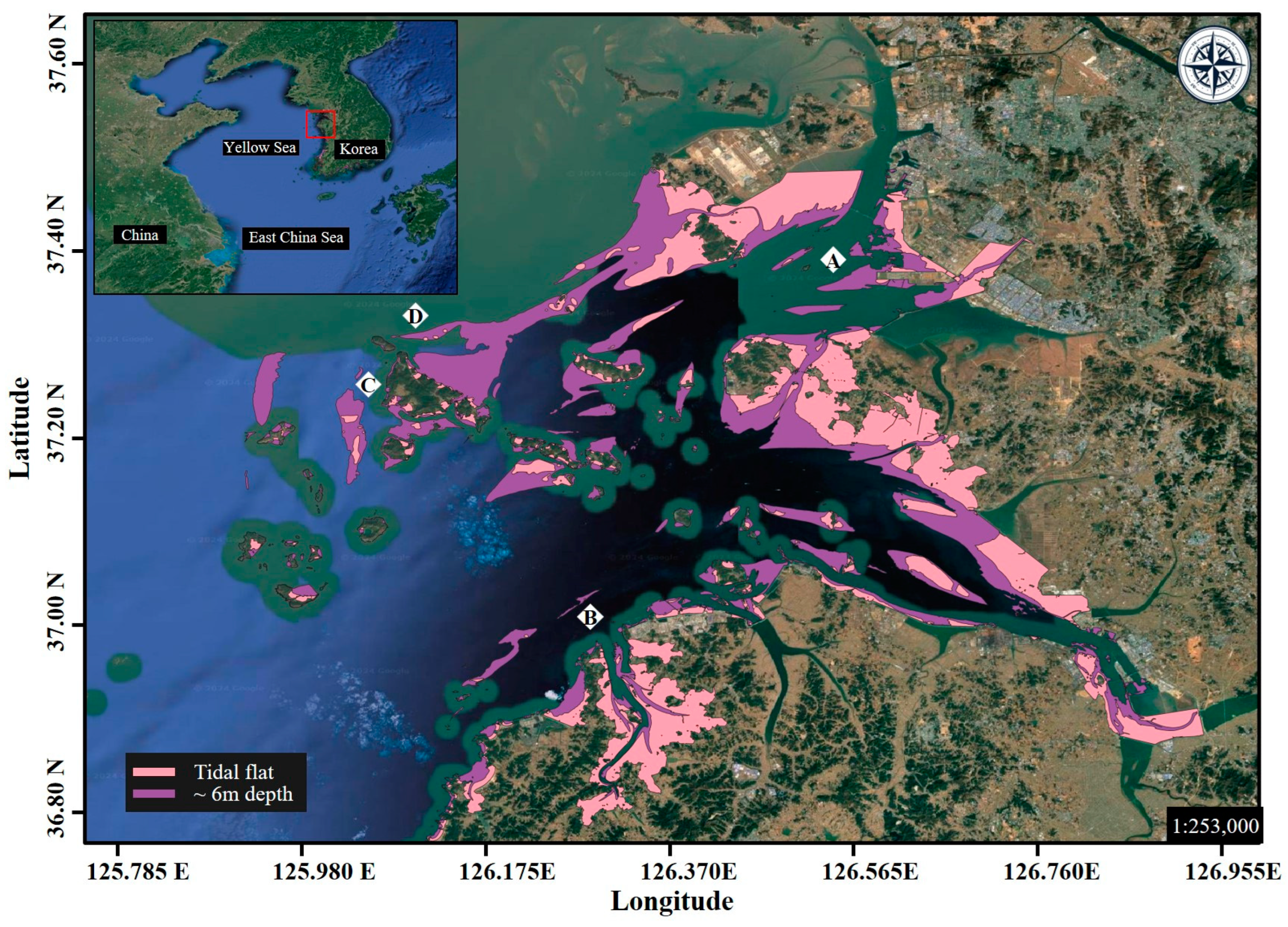
The study area, the Yellow Sea, located between the Korean Peninsula and mainland China, is a shallow marginal sea connected to the East China Sea to the south. The Yellow Sea, a shallow marginal sea with depths of an average of 44 m, is dominated by semidiurnal tides and features extensive tidal flats due to its macro-tidal environment. The Yellow Sea is influenced by the East Asian monsoon, resulting in distinct seasonal variations in temperature, wind speed, humidity, and suspended sediment dynamics [11]. Winter (November–February) is characterized by cold, dry air from Siberia, with temperatures ranging from −5 °C to −2.5 °C, while summer (May–August) brings warm, humid conditions with temperatures between 22.5 °C and 25 °C. Seasonal wind patterns show strong northwesterly winds in winter (up to 10 m/s) and weaker southeasterly winds in summer (2–3 m/s), with occasional typhoons reaching speeds of 17 m/s. Precipitation varies significantly, from 800–900 mm annually in the central Chinese region to approximately 1500 mm in central Korea and 1850 mm in Jeju Island. Suspended sediment dynamics are influenced by strong tidal currents (up to 2.5 m/s) and seasonal wind patterns, with winter storms leading to resuspension and erosion, whereas summer conditions promote sediment deposition. Large-scale coastal developments and reclamation projects have further altered tidal currents and sediment transport, impacting the natural coastal processes of the Yellow Sea.

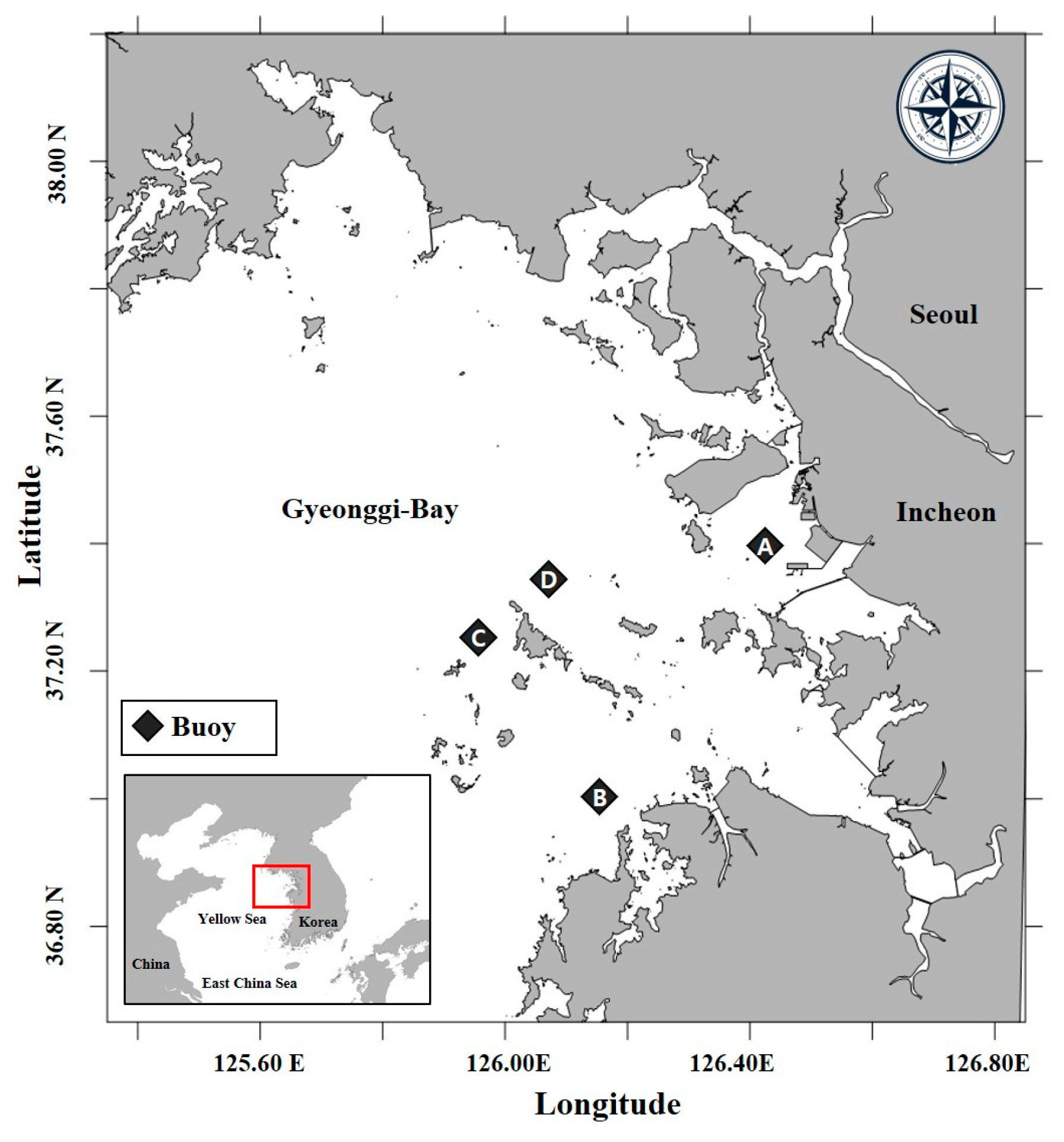
As shown in Figure 1, the Yellow Sea has the most elevated ratio of intertidal zones compared to other seas of Korea, making it the most suitable region for analyzing tidal effects and intertidal zone dynamics. It means the importance of the Yellow Sea in understanding coastal and intertidal processes, which form the foundation of this study. The intertidal zone in the Yellow Sea, which is characterized by tidal creeks and flats, plays a critical role in modulating contaminant transport and material retention [12].

2.2. Surface Boundary Condition (SBC) and Wet/Dry Treatment

The Finite Volume Community Ocean Model (FVCOM) is a three-dimensional numerical model designed to effectively simulate hydrodynamics and material transport in geographically complex structures such as estuaries [9]. The FVCOM used in this study contains an unstructured triangular mesh for accurately representing complex coastal topographies, such as intertidal zones, tidal channels, and wetlands. This advantage allows for realistic coastal modeling of localized hydrodynamic processes and improves the representation of vertical diffusion at the surface boundary. FVCOM utilizes the vertical diffusion flux (VDF) at the Ith node’s surface layer, represented by SBC:

$$VDF\left(I,1\right)=-DTI{\displaystyle \frac{S\left(I\right)+H\left(I\right)-SW\left(I\right)+RAD\left(I,1\right)-RAD(I,2)}{-DZ\left(I,1\right)D\left(I\right)}}-F(I,1)$$

(1)

This expression shows the energy balance at the ocean surface, incorporating contributions from internal time step (DTI), salinity flux (S), net heat flux (H), shortwave radiation (SW), and vertical radiative flux differences (RAD(I,1) − RAD(I,2)). DZ(I,1)D(I) represents the vertical grid spacing and water column depth, ensuring that fluxes are appropriately scaled in the vertical direction. The final term, F, adjusts for the temperature or salinity value at the surface. This equation is a boundary condition for vertical diffusion processes, explicitly considering the interplay between radiative and turbulent fluxes.

The radiative heat flux, RAD, is calculate as follows:

$$RAD=SW\times (R{e}^{{\displaystyle \frac{z}{a}}}+(1-R{e}^{{\displaystyle \frac{z}{b}}}))$$

(2)

R is the percent of the total flux associated with the longer wavelength; a and b are attenuation coefficients for different wavelength components of the shortwave irradiance. z is the thickness of the vertical layer. This formulation shows the exponential attenuation of light as it penetrates the water column, as shown by Simpson and Dickey [13].

The wet/dry treatment technique used in FVCOM is based on a three-dimensional mass conservation method. In essence, if the thickness of a vertical layer is smaller than a critical value, the region is considered an exposed intertidal zone (“dry mode”). Conversely, if the thickness exceeds the critical value, the area is regarded as covered by water (“wet mode”).

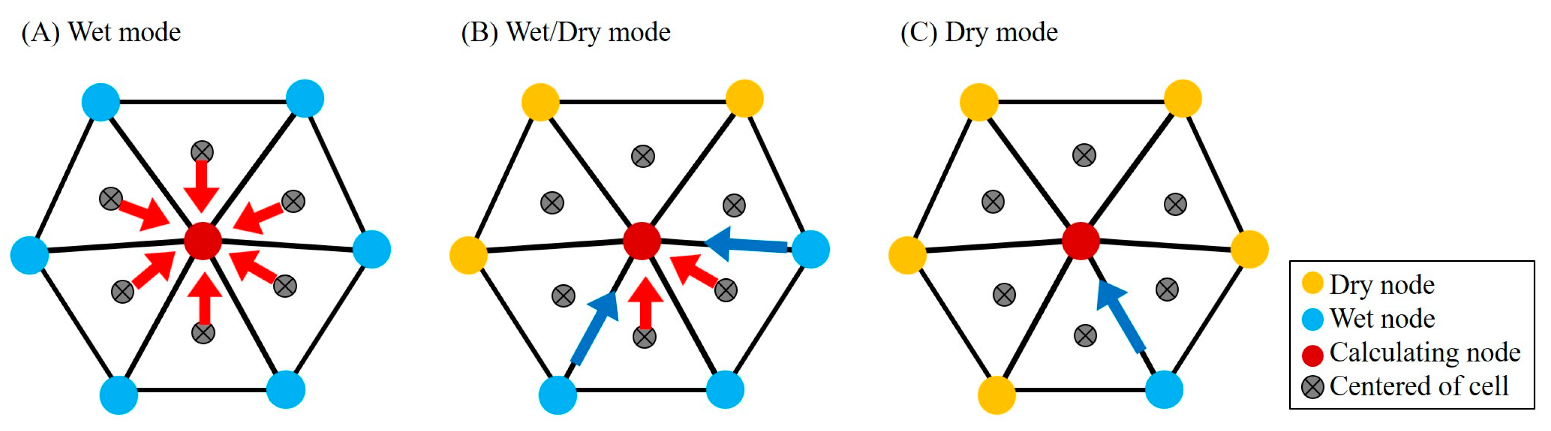
In Figure 2, all neighboring nodes are wet in (A) Wet mode, allowing adjacent nodes to uniformly influence the calculating node (red). However, in (B) Wet/Dry mode and (C) Dry mode, dry nodes (yellow) around the calculating node introduce significant challenges in maintaining numerical accuracy and stability.

Specifically, numerical errors arise when calculating temperature in areas surrounded by dry nodes for two primary reasons. First, dry nodes do not carry physically meaningful temperature values. As a result, when they are excluded from computations, the contribution of the remaining wet nodes is disproportionately amplified, leading to unrealistic values. Second, in cases where dry nodes entirely encircle the calculating node, temperature computations rely on limited information, resulting in localized numerical errors that can propagate throughout the model domain.

These wet/dry treatment limitations pose challenges for FVCOM’s application in high-resolution terrain or intermittent physical phenomena. Addressing this issue may require improvements in the numerical handling of dry nodes or adopting a weighted averaging approach that accounts for the state of surrounding nodes during temperature simulation.

2.3. Sediment Temperature Instead of SST

Kim and Cho suggested using sediment temperature as the SST in tidal flats [8]. Sediment temperature is calculated in the same way as conventional SST, and the most essential component for calculating SST is the equation for net heat flux, as shown in the formula below.

$${\mathrm{Q}}_{\mathrm{N}\mathrm{E}\mathrm{T}}={\mathrm{Q}}_{\mathrm{S}\mathrm{W}}-({\mathrm{Q}}_{\mathrm{L}\mathrm{W}}+{\mathrm{Q}}_{\mathrm{S}\mathrm{H}}+{\mathrm{Q}}_{\mathrm{L}\mathrm{H}})$$

(3)

$${\mathrm{Q}}_{\mathrm{S}\mathrm{W}}=(1-{\alpha }_{mud}){\mathrm{Q}}_{\mathrm{s}0}$$

(4)

Equation (3) represents the net heat flux Q_NET at the nodes of the numerical model, which accounts for the balance of various heat exchange components. Q_SW is the incoming shortwave radiation, primarily driven by solar energy, and serves as the primary heat source for the ocean surface. Q_LW represents the outgoing longwave radiation emitted by the surface, which acts as a cooling mechanism as the surface radiates heat back into the atmosphere. Q_SH is the sensible heat flux, which refers to the heat transfer between the ocean surface and the atmosphere due to temperature differences. Finally, Q_LH is the latent heat flux, which accounts for the heat loss associated with the evaporation of water from the ocean surface. This equation provides a comprehensive framework for quantifying the total heat flux at the surface, allowing the model to capture the complex interactions between radiation, heat exchange, and latent heat processes critical for accurately simulating surface temperature dynamics.

However, the net heat flux of sediment temperature calculates short radiation differently than before. ${\mathrm{Q}}_{\mathrm{s}0}$ is the solar radiation by the observation such as Automatic Weather Station (AWS), and ${\alpha }_{mud}$ is the albedo on the tidal flat.

$${\mathrm{Q}}_{\mathrm{L}\mathrm{W}}=[\mathsf{\epsilon }\mathsf{\sigma }{T}_a^4\left(0.4-0.05e_a^{0.5}\right)+4\mathsf{\epsilon }\mathsf{\sigma }{T}_a^3\left(T_s-T_a\right)](1-0.75C^{3.4})$$

(5)

$$e_a=0.6112\times e^{(17.67\times {\displaystyle \frac{T_a-273.15}{T_a-29.65}})}$$

(6)

$\mathsf{\epsilon }$ is the emissivity of the tidal flat sediment, $\mathsf{\sigma }$ is the Stefan–Boltzmann constant, $T_s$ is the absolute temperature of the tidal flat surface, $T_a$ is the absolute air temperature above the sediment, $e_a$ is saturation vapor pressure of the air above the sediment, and C is the amount of cloud.

$${\mathrm{Q}}_{\mathrm{S}\mathrm{H}}={\mathsf{\rho }}_a{\mathrm{C}}_{\mathrm{P}\mathrm{a}}{\mathrm{C}}_{\mathrm{h}}\left(1+\mathrm{U}\right)\left(T_s-T_a\right)$$

(7)

${\mathsf{\rho }}_a$ is the density of air, ${\mathrm{C}}_{\mathrm{P}\mathrm{a}}$ is the specific heat of air at constant pressure, ${\mathrm{C}}_{\mathrm{h}}$ is the bulk transfer coefficient for conduction, and U is the wind speed.

$${\mathrm{Q}}_{\mathrm{L}\mathrm{H}}=\mathsf{\xi }{\mathsf{\rho }}_{\mathrm{a}}{\mathrm{L}}_{\mathrm{v}}{\mathrm{C}}_{\mathrm{h}}(1+\mathrm{U})(q_m-q_a)$$

(8)

$${\mathrm{L}}_{\mathrm{v}}=(2500.84-2.35(T_s-273.16\left)\right)\times {10}^3$$

(9)

$$q_m={\displaystyle \frac{0.621{\mathrm{P}}_{\mathrm{s}\mathrm{a}\mathrm{t}}^{\mathrm{v}}}{{\mathrm{P}}_{\mathrm{a}\mathrm{t}\mathrm{m}}-(1-0.621){\mathrm{P}}_{\mathrm{s}\mathrm{a}\mathrm{t}}^{\mathrm{v}}}}$$

(10)

$\mathsf{\xi }$ is the water content of the tidal flat surface, ${\mathrm{L}}_{\mathrm{v}}$ is the latent heat of evaporation, $q_m$ is the specific humidity of saturated air at water temperature, $q_a$ is the specific humidity of air, ${\mathrm{P}}_{\mathrm{s}\mathrm{a}\mathrm{t}}^{\mathrm{v}}$ is the saturation vapor pressure at the interstitial water temperature, and ${\mathrm{P}}_{\mathrm{a}\mathrm{t}\mathrm{m}}$ is the atmospheric vapor pressure.

2.4. Sea Surface Temperature via Bulk Fomular

Instead of using observed data, it is also possible to input shortwave radiation from an atmospheric model and easily calculate net heat flux using the bulk formula. The Tropical Ocean Global Atmosphere-Coupled Ocean-Atmosphere Response Experiment (TOGA-COARE) bulk air–sea flux algorithm was developed following the international TOGA-COARE field program, which took place in the western Pacific warm pool from November 1992 to February 1993 [14]. This algorithm estimates momentum, sensible heat, and latent heat fluxes using input variables such as wind speed, SST, air temperature, and air humidity. It also includes subroutines and functions to handle near-surface temperature gradients in the ocean, making it adaptable to a variety of environmental conditions. One of the key advantages of the COARE algorithm is its simplicity and fixed parameterization, which enables fast and efficient calculations. For example, Song demonstrated the importance of relative wind speed in improving the accuracy of turbulent heat flux estimations using the COARE bulk algorithm in the Bohai Sea, highlighting its applicability to various regional conditions [15]. While this is a general benefit of bulk formulas, the COARE algorithm leverages this strength to provide high accuracy and computational efficiency, making it particularly effective for high-resolution coastal and oceanic models in estimating heat and momentum fluxes.

COARE aims to calculate sensible and latent heat flux to determine net heat flux. This process differs from those Kim and Cho proposed for deciding sediment temperature [8].

$${\mathrm{Q}}_{\mathrm{S}\mathrm{H}}={\mathsf{\rho }}_a{\mathrm{C}}_{\mathrm{P}\mathrm{a}}{\mathrm{C}}_{\mathrm{h}}\mathrm{U}\left(T_s-T_a\right)$$

(11)

$${\mathrm{Q}}_{\mathrm{L}\mathrm{H}}={\mathsf{\rho }}_a{\mathrm{C}}_{\mathrm{P}\mathrm{a}}{\mathrm{C}}_{\mathrm{h}}\mathrm{U}\left(T_s-T_a\right)$$

(12)

Longwave and shortwave radiation are also directly inputted from atmospheric models, inevitably leading to differences in the results when calculating sediment temperature.

2.5. Final Algorithm

Different thermal and material exchange mechanisms are applied depending on the coastal region, such as the intertidal zone. Terrestrial areas, which do not come into direct contact with seawater, are primarily governed by thermal processes based on sediment temperature. In tidal flats and intertidal zones, periodic wetting and drying occur due to tidal variations. Modified SBC and BBC are applied to account for these dynamic processes. On the other hand, regions that remain constantly submerged rely on the bulk formula to calculate air–sea heat and momentum fluxes. These approaches allow for precise simulation of air–sea and sediment interactions, enabling accurate representation of thermodynamic processes in coastal areas.

In coastal environments, the dry and wet zones remain consistently exposed or submerged, respectively. However, in the intertidal zone, where the state alternates between dry and wet due to tidal variations, a single thermal equation is insufficient to simulate the dynamic processes accurately. This study introduces a newly defined Heating Limit Depth (HLD) and presents an approach in which the surface temperature is substituted with the sediment temperature when the depth falls below a specified critical threshold (Figure 3). This approach enables precise calculation of surface temperature variations influenced by HLD, facilitating more accurate simulation of thermodynamic changes in complex environments such as intertidal zones.

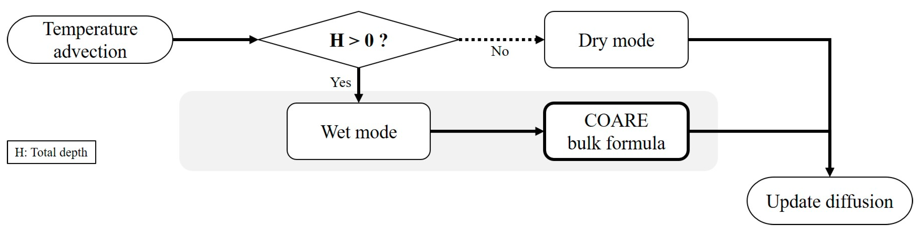
Figure 4 illustrates the final procedure used within the numerical model to calculate the advection and diffusion terms for SST. The process begins by determining whether a given computational node is in “dry mode” or “wet mode” based on the local water depth and tidal conditions. If the node is classified as “dry mode”, the heat flux and SST are calculated using sediment temperature dynamics, indicating the absence of direct water coverage. For nodes in “wet mode”, the algorithm incorporates the “COARE bulk formula” to compute air–sea heat fluxes, including components such as shortwave radiation, longwave radiation, sensible heat flux, and latent heat flux. These fluxes are then integrated with the governing equations of the model to accurately simulate the advection and diffusion of heat across the water surface. This dynamic switching between modes ensures that both wet and dry zones are appropriately managed, allowing for precise representation of thermal processes in complex environments such as tidal flats and intertidal zones. The flexibility and robustness of this approach enhance the model’s capability to simulate realistic heat transport and exchange processes in coastal systems.

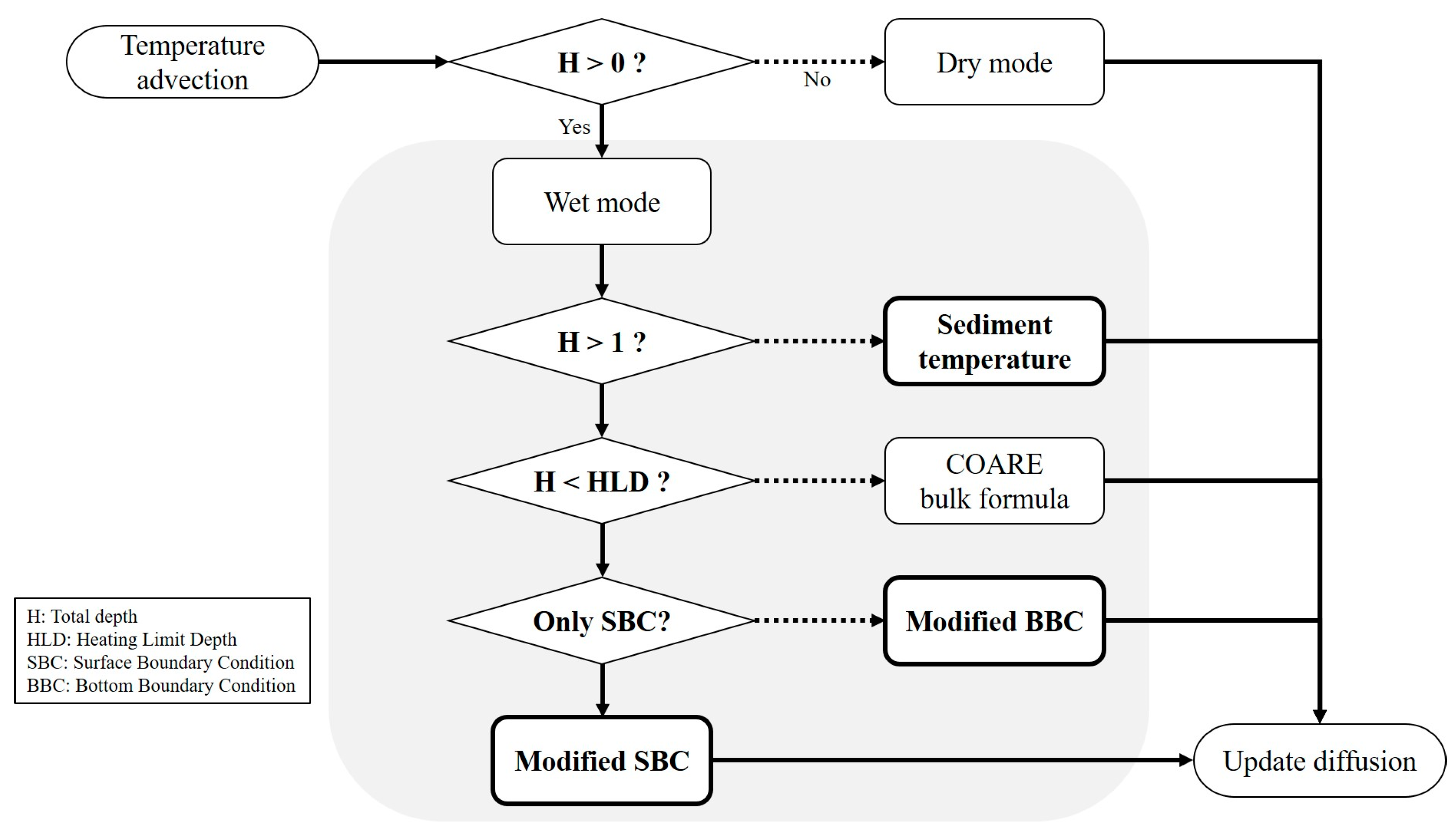
Figure 5 shows that the updated algorithm introduces additional decision-making steps to enhance the management of thermal processes in coastal and intertidal zones, building upon the original framework. While the original algorithm differentiated between “dry mode” and “wet mode” and applied the “COARE bulk formula” for heat flux calculations in the wet mode, the new approach incorporates multiple conditions to account for varying depths and surface dynamics. In the updated algorithm, if the node is in “wet mode”, the model first checks if the total water depth (H) exceeds 1 m. If so, the heat flux is calculated using sediment temperature, accounting for shallow water dynamics. For depths below 1 m, the algorithm introduces a further condition by comparing H with the HLD. If H is less than HLD, the COARE bulk formula is applied, ensuring an accurate representation of air–sea fluxes. For cases where SBC alone is insufficient, the algorithm incorporates a “modified BBC” to refine heat flux calculations. Finally, in scenarios requiring adjustments at the surface, a “modified SBC” is applied. These enhancements allow the model to dynamically adjust to varying environmental conditions, improving the accuracy of thermal simulations across different depth regimes, particularly in shallow and intertidal zones where traditional methods are insufficient. This refined approach ensures a more precise representation of heat exchange and sediment interactions.

2.6. Experiment Design and Model Configuration

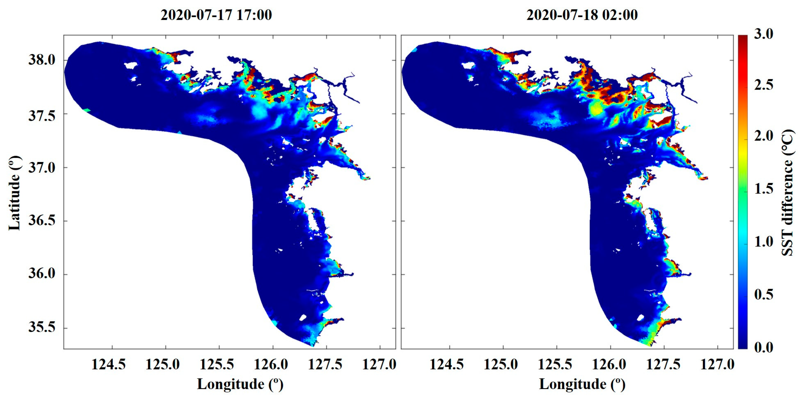
This study prepared two models to evaluate the effects of different approaches to calculating SST in coastal regions. The first model utilizes the conventional model scheme presented in Figure 4, while the second model employs the improved model scheme shown in Figure 5. The SST calculated from each model is obtained, and their differences are analyzed. The results focus on the summer season, as the differences between solar radiation and geothermal heat during this period lead to significant SST variations, increasing the potential errors of the numerical model. Therefore, the simulation period was prioritized for the summer to analyze these errors and evaluate the effectiveness of the improved algorithm.

The grid resolution was set to a maximum of less than 150 m, with the open boundary resolution at approximately 2 km. Furthermore, following the methodology of Gu et al., an unstructured grid system accounting for tidal channels was used to refine the coastal grid [12]. This configuration was designed to more effectively analyze the intertidal and coastal zones’ physical characteristics and temperature variations.

The model’s open boundaries were set based on Korea’s territorial sea limits to concentrate calculations on the intertidal and coastal zones. While wider open boundaries generally reduce numerical errors caused by external forces, this study constrained the open boundaries to the territorial limits to focus on analyzing surface temperature responses, given limited computational resources. The open boundary conditions for the background model were derived from Finite Element Solution (FES) 2014 [16], which operated a global tidal numerical model assimilating satellite-observed sea surface height data. These conditions incorporated only the eight major tidal components (M₂, S₂, K₂, N₂, K₁, O₁, P₁, Q₁) that significantly impact GGB. After completing the horizontal grid configuration of the background model, these were directly interpolated to the open boundary nodes, and the tidal boundary input data were organized.

Based on the Korea Operational Oceanographic System (KOOS), this study utilizes initial and boundary conditions derived from the KOOS ocean model (2 km), which is designed to provide accurate predictions for regional and coastal waters. The atmospheric forcing was prepared by interpolating meteorological outputs from the KOOS atmospheric model (4 km), ensuring consistency and high-resolution integration between oceanic and atmospheric processes. This approach aligns with existing efforts to develop realistic numerical models that effectively couple large-scale ocean models with localized coastal dynamics, as demonstrated in previous works [17]. The coupling between these systems enables a more precise representation of surface forcing and boundary conditions, particularly in complex coastal environments.

3. Results and Analysis

3.1. SST Changes Induced by Algorithm Modification

Figure 6 shows the model results in the Yellow Sea at two selected times from June to August 2020. The contours in Figure 6 represent the differences in SST before and after improving the coastal SST algorithm. This result represents the difference between the SST estimated in the existing model and the SST in the model using the improved algorithm. If this SST difference in Figure 6 is positive, it means that the improved algorithms in this study have a higher SST than the existing SST simulation. This difference in change only responds to the intertidal zone. This means that the area of SST difference distribution is similar to the intertidal zone, and the SST simulation is approached in a similar process as the wet/dry treatment. The analysis focuses on the timeframes in mid-July when the maximum and minimum difference ranges occurred in the intertidal zones. In Figure 6, the legend was limited to 0 to 3 °C to check whether the SST algorithm improvement effect appeared focused on the intertidal zone. Still, the actual SST difference in Gyeonggi-Bay reached 5.6 °C. In the intertidal zones of the Yellow Sea, regions with significant SST differences represent the thermal transport and mixing processes influenced by tidal currents. The left panel in Figure 6 shows relatively low SST difference areas in parts of the Yellow Sea, which can be interpreted as effects of tidal currents and reduced solar radiation during that period. This phenomenon is explained by sea breezes and land breezes, where the ocean’s higher heat capacity compared to land leads to slower heat absorption and release, stabilizing SST fluctuations on the nearby coasts. Therefore, the right panel depicts areas with increased SST in some intertidal zones, likely related to characteristics of sea breezes.

3.2. SST Validation with the Final Algorithm in Gyeonggi-Bay of the Yellow Sea

The validation of results before and after the SST algorithm improvement was conducted using operational observation buoys in the Yellow Sea to figure out consistency between the model results and the observations (Figure 7).

The diamond symbols in Figure 7 represent buoy observation sites. Although buoys cannot be installed directly in intertidal zones, they are placed near islands or adjacent to navigation channels, making them practical for monitoring variability in coastal environments. Additionally, the observation points are located near the central part of the Yellow Sea, providing a suitable environment for analyzing coastal SST changes during the validation period in this study.

Figure 8 shows the time series of SST variations at four observation points (A, B, C, D) from 15–18 July 2020. The red dots represent the observed SST. The black line indicates the model results based on the original algorithm, and the blue line represents the model results using the improved algorithm. At observation point A, located closest to the intertidal zone, the agreement between observed data and model results is relatively high, with the improved algorithm (blue line) showing results closer to the observations than the original algorithm (black line). At observation point B, situated near a navigation route, the improved algorithm demonstrates an apparent reduction in errors compared to the original algorithm, particularly in peak values. At observation point C, located near offshore islands, the improved algorithm more accurately reproduces the patterns of the observed data and better reflects SST variations than the original algorithm. Finally, at observation point D, similar to the other locations, the improved algorithm reduces discrepancies with the observed data and better captures changes associated with tidal cycles. Overall, the improved algorithm (blue line) demonstrates a higher level of agreement with observed data, enabling a more accurate representation of SST variability compared to the original algorithm. This indicates that the improved algorithm is effective in simulating SST variations in intertidal and coastal regions.

Figure 8 presents a time series of less than a week to spotlight significant differences. However, in part of Figure 8, it is not easy to find improvement between “Before” and “After”. Therefore, the Root Mean Square Error (RMSE) was analyzed for the entire simulation period to compare each experiment. Based on RMSE via algorithm improvement, Buoy “A” reduced from 0.54 °C to 0.42 °C, approximately a 0.08 °C decrease. Buoy “B” exhibited a decline from 0.50 °C to 0.43 °C (0.07 °C reduction), while Buoy “C” showed a reduction from 0.34 °C to 0.28 °C (0.06 °C decrease). The most significant improvement was observed in Buoy “D”, where RMSE decreased from 0.42 °C to 0.32 °C (0.1 °C decrease). On average, the RMSE decreased by approximately 0.08 °C, indicating an overall improvement of about 19%. Additionally, results were verified by observed data in a time series and compared using the skill score (SS) suggested by Murphy [18]. When assuming the reference simulation as an absolute value of observation, the SS can be explained as a dimensionless number ranging between 0 and 1, indicating how well the prediction replicates the actual observation. In other words, the closer the SS is to positive 1, the higher the correlation and accuracy are about the true observation.

Table 1. Comparison of skill score (SS) between basic and modified simulated sea surface temperatures (SSTs) at four buoy locations (A, B, C, D). The “Before” column represents results from the original algorithm, while the “After” column shows results from the improved algorithm.

Buoy Name	Before	After
A	0.34	0.59
B	0.59	0.69
C	0.75	0.84
D	0.72	0.85

presents the skill scores between observed data and model results at four observation points (A, B, C, D) using the original algorithm and the improved algorithm. It can be confirmed that the improved algorithm exhibits a higher correlation with the observations compared to the original algorithm at all points. Notably, observation points near intertidal zones (Buoy A) demonstrated up to a 0.25 improvement of SS, confirming that the improved algorithm reproduces SST variations in intertidal areas more accurately. This indicates that the improved algorithm can represent physical processes more precisely, enhancing numerical modeling performance in intertidal and coastal regions.

To evaluate the accuracy of SST in tidal flat areas, statistical analyses were performed using data from buoys, which are indicated as white diamonds in Figure 1. Since operational buoys cannot be installed and maintained directly in tidal flats or ship channels, they are placed as close to these regions as possible. Given that the observed improvements were evident at these buoy locations, it is reasonable to infer that similar improvements would also apply in tidal flat areas. This suggests that our approach effectively enhances the accuracy of SST mapping, even in environments where direct measurements are challenging.

4. Discussion

This study confirmed significant SST improvement effects in the Yellow Sea, where the intertidal zone is extensive, by applying an improved algorithm that separates the heat capacity and diffusion coefficients between air–sea and intertidal–coastal systems. These improvement effects are more pronounced in regions with tidal flats, freshwater discharge, and tidal creeks, demonstrating that the intertidal processing technique contributes to enhanced simulation accuracy.

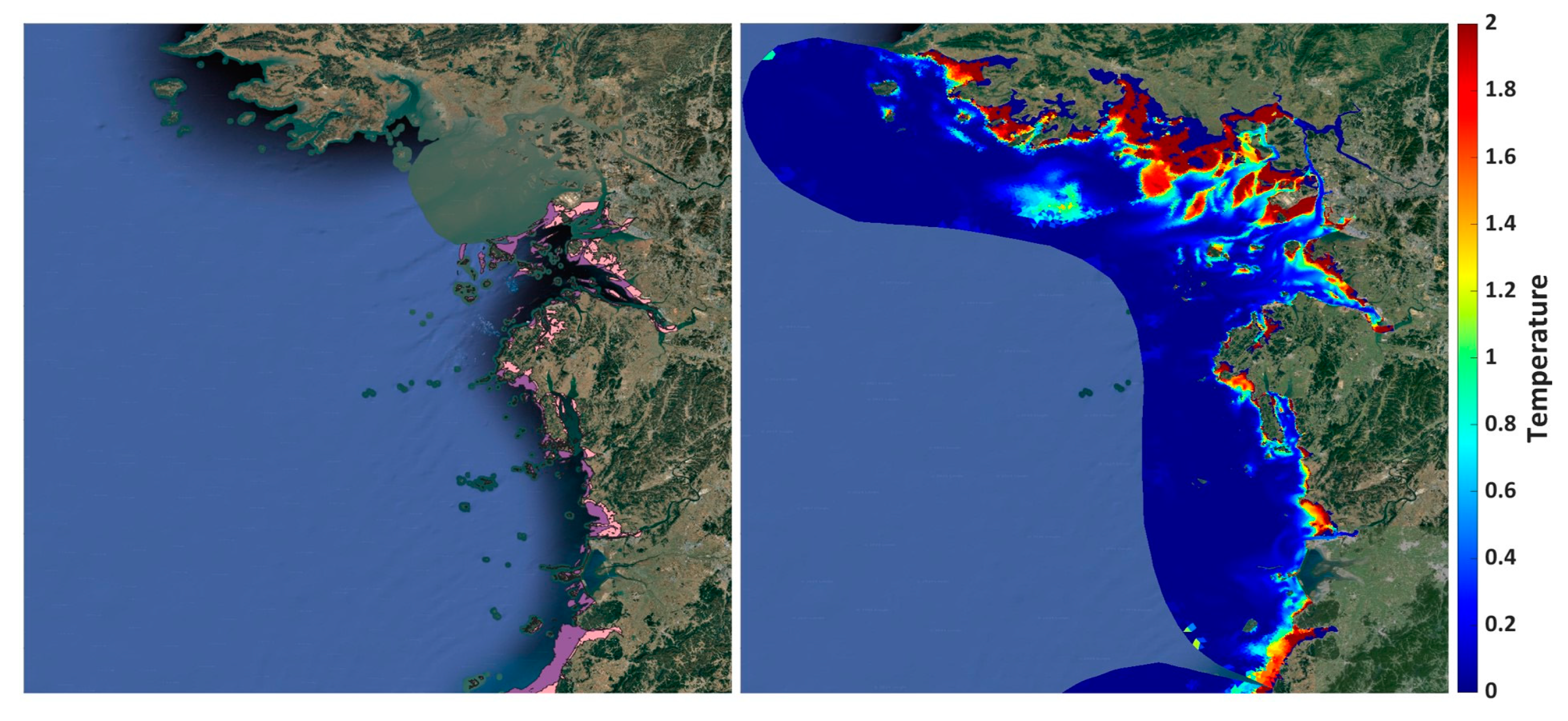
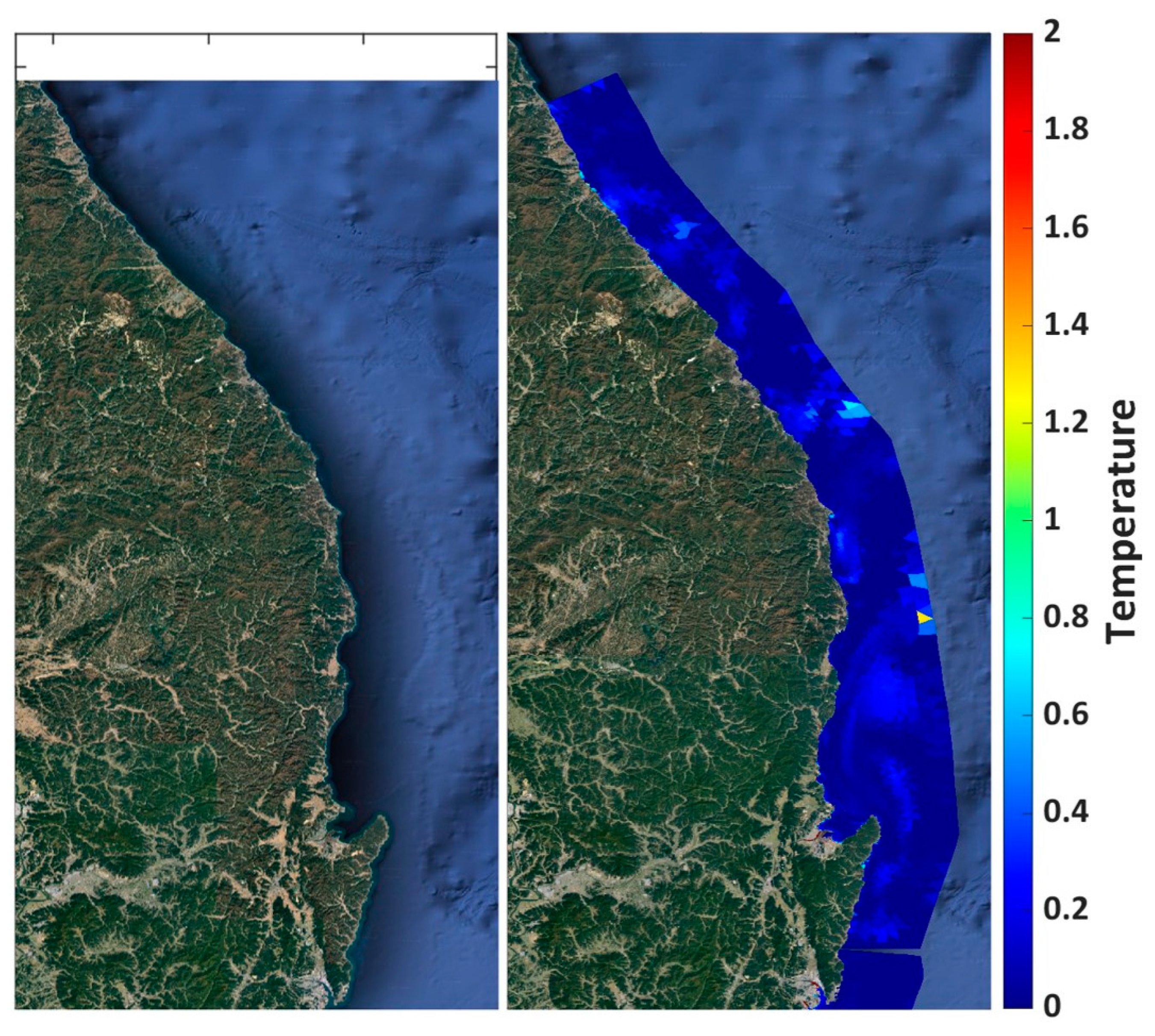
Figure 9 compares the SST distribution via simulated results with the actual tidal flat survey [19]. This comparison confirms that the algorithm improvements proposed in this study can more accurately reproduce SST variations in tidal flats. The improvement effects are particularly evident in tidal flats with a water depth of less than 6 m, as the segmentation of heat capacity and diffusion coefficients were refined to suit the intertidal environment. Therefore, the algorithm developed in this study significantly contributes to the numerical modeling of coastal areas and has potential applications in coastal ecosystems. The improved model’s effect on SST simulations is evident, and the energy balance is transferred to adjacent nodes through wet/dry treatment. Moreover, due to intense tidal currents in the Yellow Sea, SST changes were observed even near the open boundary.

Additional experiments were conducted to verify whether the improved algorithm applied in this study is effective exclusively in tidal flats. Two additional simulations were conducted for the summer season (June to August 2020) using coastal models (East and South Seas) constructed under identical conditions.

The South Sea has numerous islands and an extensive intertidal zone with a water depth of less than 6 m. These characteristics contributed to significant improvements in SST representation within the intertidal zone following the algorithm enhancement (Figure 10). In the South Sea of Korea, the tidal amplitude during spring tides is typically around 3.351 m compared to the Yellow Sea [20], where it can reach up to 10 m [11]. As a result, the intertidal zone in the South Sea is relatively narrow. However, the algorithm enhancement demonstrates its potential to improve SST accuracy in this region despite the narrow area of SST improvement compared to the Yellow Sea.

The East Sea is relatively deeper than the Yellow Sea and the South Sea, so the effect of improving the SST through algorithm improvement is not significant (Figure 11). Nevertheless, the occurrence of several localized temperature differences indicates the need for further study to adjust the sensitivity of parameters in the sediment temperature calculation process.

According to the tidal flat area survey [18], 83.8% of the tidal flats are distributed in the Yellow Sea and 16.2% in the South Sea. These tidal flats cover approximately 2482 km², which accounts for 5.05% of the total land area of South Korea. This is important for improving numerical modeling to achieve a more comprehensive scientific analysis and understanding of the region, as its vast area is comparable to the total land area of coastal administrative cities. Furthermore, the intertidal dry ratio in the numerical model was confirmed to be about 15.8%, demonstrating that the improved algorithm, which accurately reflects intertidal characteristics, contributed to the enhanced model performance.

The intertidal zone is quite sensitive to the influence of tides and freshwater inflow. In the Yellow Sea model domain, freshwater inflow from the Han River exceeds 28 × 10⁹ m³/y, while the Geum River contributes around 7 × 10⁹ m³/y, and the tidal range exceeds 6 m. In contrast, the South Sea is less affected by tides and freshwater inflow. Furthermore, the East Sea is dominated more by currents than tides. A model scheme that can be simultaneously applied to such diverse coastal regions while showing apparent improvement effects has good practical significance.

This study conducted a primary sensitivity analysis of HLD before its implementation. Sensitivity experiments were conducted using coastal models, focusing on the optimized HLD. Results indicated that the optimal HLD decreased in the Yellow Sea, corresponding to the higher impacts of tides and freshwater inflows in the Yellow Sea compared to the other regions. The revised ocean model’s improved vertical diffusion terms for SST proved effective mainly in tidal flat areas, while the effect diminished in broader coastal zones with depths exceeding an average of 5 m.

The results of this study emphasize the importance of resolving SBC and BBC to improve SST predictions in coastal regions. The findings indicate that boundary adjustments, such as optimized depth limits, are critical in reducing SST biases, especially in tidal flats. This approach aligns with insights from Choi and Lippmann, which addressed similar boundary-related issues in ecosystem models [21]. Choi and Lippmann demonstrated that unrealistic oligotrophic conditions in shallow coastal waters are caused by poorly resolved bottom boundary conditions, resulting in nitrogen loss that disrupts ecological balances [21]. Their expanded ecosystem model, which incorporates denitrification and nitrogen fixation, focuses on optimized parameterization to simulate local dynamics accurately. Drawing parallels, this study’s SBC/BBC modifications and ecological adjustments by Choi and Lippmann both highlight the necessity of resolving boundary processes to improve model performance in coastal systems [21]. Integrating thermal and ecological approaches could further enhance coastal modeling by addressing coupled dynamics between heat flux and nutrient cycles, paving the way for more robust and realistic ocean forecasting systems.

This study focuses on improving numerical model accuracy through physical algorithms and sensitivity estimations. Bharti et al. and Kim et al. address the optimization of observation networks to detect local characteristics of ocean variables, including temperature and salinity [22,23]. Both studies highlight the importance of developing methodologies applied to specific regional or operational needs. For instance, Kim et al. indicate that optimal solutions for buoy placement align with the necessity of refining input parameters in numerical models to detect local dynamics, such as tide and current influences [23]. These approaches suggest that integrating optimized observational strategies with model adjustments could further improve the accuracy of ocean forecasting systems, ensuring more reliable predictions of SST and other necessary oceanographic variables.

The development of operational forecasting systems suggests the integration of atmospheric models to improve SST predictions in coastal and tidal flat regions. Also, Lee et al. emphasize the potential of satellite-based approaches, such as high-resolution Landsat 8 data, to grab spatial and seasonal variability of SST near tidal flats [24]. A key distinction between these methods is their resolution: while relatively coarse spatial resolutions limit atmospheric models, they excel in capturing dynamic processes over broader scales. Conversely, satellite observations provide high spatial resolution, making them particularly effective for understanding localized variation, such as the sharp horizontal SST gradients near tidal flats.

This suggests that the choice between atmospheric models and satellite data should consider the target resolution and application. For large-scale forecasting and continuous temporal coverage, atmospheric models remain indispensable. However, integrating satellite-derived data can complement these models by refining boundary conditions or validating localized SST patterns. Future improvements could focus on hybrid approaches, leveraging both methodologies’ strengths to balance spatial resolution and dynamic forecasting capabilities, ensuring more accurate and adaptive coastal SST predictions.

5. Conclusions

This study proposes improvements aimed at significantly enhancing SST predictions in regions dominated by tides, freshwater inflows, and intertidal zones. In particular, this approach is expected to have a more pronounced effect in estuary models, where intertidal zones account for over 30% of the model domain. However, a limitation of this study is the potential for overestimation under specific conditions, such as closed Dry Cell/Node in the model domain. This indicates the need for clear criteria to define the maximum allowable proportion of dry zones. Also, further validation regarding seasonal variability is necessary, which will provide a deeper understanding of modeling performance in intertidal and coastal environments. Notably, the impact of improved intertidal processing techniques is relatively constrained in regions such as the East Sea, where intertidal zones are nearly absent. This ultimately suggests the need for region-specific modeling approaches. Finally, the improved air–sea interaction processing in the intertidal zone technique is expected to significantly improve model prediction performance in intertidal zones. This method will substantially contribute to future research and applications in coastal modeling.