Article

Coastal Ecosystem Services in Urbanizing Deltas: Spatial Heterogeneity, Interactions and Driving Mechanism for China’s Greater Bay Area

1
School of Land Science and Technology, China University of Geosciences, Beijing 100083, China
2
Real Estate Registration Center, Ministry of Natural Resources, Beijing 100034, China
*
Author to whom correspondence should be addressed.
These authors contributed equally to this work.
Water 2025, 17(24), 3566; https://doi.org/10.3390/w17243566
Submission received: 18 November 2025 / Revised: 6 December 2025 / Accepted: 9 December 2025 / Published: 16 December 2025
(This article belongs to the Section Oceans and Coastal Zones)

Abstract

As critical ecosystems, coastal zones necessitate the identification of their ecosystem service values, trade-off/synergy patterns, spatiotemporal evolution, and driving factors to inform scientific decision-making for sustainable ecosystem management. This study selected the coastal zone of the Guangdong-Hong Kong-Macao Greater Bay Area (GBA) as the research region. By incorporating land-use types such as mangroves, tidal flats, and aquaculture areas, we analyzed land-use changes in 1990, 2000, 2010, and 2020. The InVEST model was employed to quantify six key ecosystem services (ESs): annual water yield, urban stormwater retention, urban flood risk mitigation, soil conservation, coastal blue carbon storage, and habitat quality, while spatial correlations among them were examined. Furthermore, Spearman’s rank correlation coefficient was used to assess trade-offs and synergies between ecosystem services, and redundancy analysis (RDA) combined with the geographically and temporally weighted regression (GTWR) model were applied to identify driving factors and their spatial heterogeneity. The results indicate that: (1) Cultivated land, forest land, impervious surfaces, and water bodies exhibited the most significant changes over the 30-year period; (2) Synergies predominated among most ecosystem services, whereas habitat quality showed trade-offs with others; (3) Among natural drivers, the normalized difference vegetation index (NDVI, positive effect) and evapotranspiration were critical factors. The proportion of impervious surfaces served as a key land-use change driver, and the nighttime light index emerged as a primary socioeconomic factor (negative effect). The impacts of drivers on ecosystem services displayed notable spatial heterogeneity. These findings provide scientific support for managing the supply-demand balance of coastal ecosystem services, rational land development, and sustainable development.

1. Introduction

Coastal zones, as transitional areas where land and sea interact, represent the most biologically complex and resource-rich regions on Earth’s surface. Characterized by high species diversity and intensive human activities, these zones significantly influence both ecological systems and socio-economic dynamics. Current coastal research primarily focuses on: land-use change [1], resource exploitation, ecosystem services, integrated coastal zone management, coastal resilience [2], and spatial planning. Such studies are critical for coastal conservation, spatial expansion of resource utilization, enhanced management efficiency, and promoting land-sea coordinated development. Coastal blue carbon, a key component of blue carbon sinks [3], plays a pivotal role in global carbon cycles. It delivers multifaceted benefits: providing habitats for marine organisms to maintain biodiversity; sequestering carbon to regulate climate and mitigate warming; buffering wind and waves to protect shorelines; and supplying raw materials and aesthetic value to support fisheries and tourism. Technologically, high-resolution remote sensing and GIS enable real-time monitoring of blue carbon ecosystem dynamics [4], while carbon stock studies provide theoretical foundations for assessing sequestration capacity. Internationally, blue carbon trading markets are being explored to quantify carbon sink functions [5], offering economic incentives for coastal ecological protection. Mangroves, as dominant vegetation in tropical/subtropical coastal zones, constitute essential blue carbon reservoirs. They provide critical services including carbon sequestration, storm surge mitigation [6], water purification, and biodiversity conservation. Research on mangroves enriches coastal studies and is vital for maintaining ecosystem stability.
Ecosystem services (ES) refer to the conditions and utilities formed and sustained by ecosystems that support human survival. Since Costanza et al. (1997) [7] conceptualized ES, research has expanded globally. ES are categorized into provisioning, regulating, supporting, and cultural services [8], each playing distinct roles in ecological and socio-economic activities. Ecologically, ES maintain balance; economically, they provide timber, food, and raw materials while regulating climate, hydrology, and soil stability. They also offer aesthetic and scientific value through natural landscapes. However, industrialization and anthropogenic pressures increasingly threaten ecosystems. Sea-level rise from global warming exceeds coastal ecosystems’ adaptive capacity [9], while unsustainable land use has degraded approximately 60% of ES [10]. Thus, restoring ES functionality and improving management are urgent priorities to enhance human well-being.
Ecosystem services (ES) have garnered widespread societal attention, emerging as a prominent research focus in contemporary interdisciplinary studies. Current investigations into ES primarily concentrate on four interconnected dimensions: First, the quantification of ES values, which employs methods such as the equivalent factor method (based on per-unit-area ecosystem value) [11], the benefit transfer method, and biophysical process-based modeling to monetize intangible benefits like carbon sequestration and flood mitigation, thereby informing decision-making for natural resource management. Second, the analysis of ES supply-demand balance, where scholars clarify spatial distributions of supply and demand zones [12], assess supply-demand budgets [13], and examine ES flows [14]—including their directions, characteristics, and efficiency (quantified via metrics like transfer volume and efficiency) [15]—to optimize resource allocation. Third, the exploration of trade-offs and synergies among ES, utilizing approaches such as the Ecosystem Service Change Index (IESC), correlation analysis (e.g., Spearman’s rank correlation), and spatial statistics [16] to characterize interactions between services, whether reinforcing (synergies) or conflicting (trade-offs). Fourth, the investigation of ES spatial heterogeneity and its drivers, involving spatial autocorrelation analysis, dynamic modeling, and geospatial techniques (e.g., multi-scale geographically weighted regression [17], geographically weighted regression (GWR), and GTWR to map ES distribution patterns and identify drivers of spatiotemporal variability, including natural and anthropogenic factors. Collectively, these research foci provide critical insights for enhancing ecosystem management, sustaining human well-being, and guiding sustainable development strategies.
Coastal ecosystems, as vital yet fragile ecological zones, play a critical role in maintaining biodiversity and providing essential services while facing significant anthropogenic and environmental pressures. These systems are increasingly threatened by natural hazards such as sea-level rise and storm surges, compounded by human activities including rapid urbanization, large-scale land reclamation, industrial wastewater discharge, and overfishing [18], which degrade ecological functions and destabilize their resilience and sustainability. In China, research on coastal ecosystems has transitioned from qualitative assessments to quantitative analyses, focusing on ecosystem service valuation (e.g., equivalent factor methods and biophysical modeling), spatiotemporal dynamics via remote sensing and GIS [19], supply-demand balance, ecological security patterns, ecological network identification [20], ecosystem resilience, service trade-offs/synergies, and driving factors. These advancements inform strategies for ecological compensation, service value realization, and integrated coastal management to enhance human well-being and ecosystem coupling [21]. Current studies predominantly concentrate on regions like the Yellow Sea/B Bohai Sea, the Yangtze River Delta, and Hainan’s coasts. The GBA, a dynamic economic hub within the Pearl River Delta, exemplifies these challenges due to extensive reclamation since the 1990s, which has drastically altered coastlines and land-use patterns. As a critical node for ecological research, the GBA’s coastline evolution and socio-economic pressures underscore its representativeness in addressing coastal ecosystem sustainability amid rapid urban growth.
Despite an increasing number of coastal ES studies in China, research focusing on the integrated coastal (marine + terrestrial) ES dynamics of rapidly urbanising megaregions—such as the GBA—remains limited. Existing studies often: (i) use terrestrial land-cover classifications that omit coastal land types (e.g., tidal flats, aquaculture), (ii) analyse ES at single time points or short intervals, (iii) provide limited mechanistic interpretation of socio-ecological drivers at fine spatial scales, and (iv) under-report model parameter sources and uncertainty [22,23]. To address these gaps, this study (1) refines coastal land-use classification by explicitly including mangroves, tidal flats and aquaculture; (2) quantifies six coastal ES across four decadal epochs (1990, 2000, 2010, 2020) to capture multi-decadal trajectories; (3) combines spatial autocorrelation, trade-off/synergy analysis, RDA and GTWR to identify spatially heterogeneous drivers and interpret mechanisms; and (4) documents model inputs, parameter sources and uncertainty assessment to improve reproducibility and comparability with other coastal InVEST studies. These advances make the GBA case useful as a methodological and empirical reference for urbanizing deltas worldwide.

2. Materials and Methods

2.1. Study Area Overview and Data Sources

The Guangdong-Hong Kong-Macao Greater Bay Area (GBA), located along China’s southern coast (21°25′ N–24°30′ N, 111°12′ E–115°35′ E), encompasses the Hong Kong Special Administrative Region, Macao Special Administrative Region, and nine prefecture-level cities in Guangdong Province (Guangzhou, Shenzhen, Zhuhai, Foshan, Huizhou, Dongguan, Zhongshan, Jiangmen, and Zhaoqing), covering a total area of 56,000 km2. Characterized by a subtropical monsoon climate with a mean annual temperature of 22.5 °C and mean annual precipitation ranging from 1500 to 2500 mm, the GBA sits on delta alluvial plains with mountainous areas in the north. Its ecosystems are rich in biodiversity, with mangroves, seagrass beds, and other coastal ecosystems providing critical services such as water purification and storm surge mitigation. Economically, the GBA is highly dynamic, featuring thriving port shipping, clustered marine industries, and intensive coastal development and urban construction, accelerated by large-scale land reclamation since the 1990s. Since 2000, rapid economic growth and urban expansion have significantly altered land-use patterns [24], weakening regional ecosystem service functions.
To better highlight the spatiotemporal changes in ecosystem services in the GBA’s coastal zone, this study defines the coastal research boundary as follows: the terrestrial component includes a 10-km buffer zone extending inland from the GBA coastline, while the marine component covers the area extending inland from the 6-m isobath. To refine this boundary, we extracted the 6-m isobath from DEM data, adjusted its scope based on dataset coverage by removing land-crossing segments and smoothing irregular edges, and combined it with a 10-km terrestrial buffer zone (with the continental coastline as the reference) to form the final closed study area. A schematic of the study region is shown in Figure 1.
The data used in this study primarily include basic geographic information, land use data, soil and hydrological data, topographic data, and vegetation index data for the years 1990, 2000, 2010, and 2020. The specific data sources are listed in Table 1. All datasets were projected to a unified coordinate system using ArcGIS 10.8.2, and the cell size was standardized to 30 m × 30 m through resampling.

2.2. Land Use Change Analysis

The annual China land cover dataset (CLCD) was utilized, which the overall accuracy was stable and satisfactory (76.45% OA < 82.51 %), with average OA of 79.30% ± 1.99% [25]. This study integrated coastal-specific land use categories (e.g., tidal flats, mangroves, aquaculture) to classify the GBA’s coastal zone into 10 types: cropland, forest, grassland, waterbody, bare land, impervious surface, marine, tidal flat, mangrove, and aquaculture. Land use data for 1990, 2000, 2010, and 2020 were extracted to quantify spatiotemporal trends and shifts. Transition matrices and Sankey diagrams were generated to visualize land use changes and inter-category fluxes over three decades.

2.3. Ecosystem Service Value Assessment

Guided by principles of research significance and data accessibility, this study selects six ecosystem service types for valuation: annual water yield (WY), urban rainwater retention (UR), urban flood risk mitigation (UF), soil conservation (SC), coastal blue carbon (BC), and habitat quality (HQ). Quantification of these services was implemented using the InVEST (Integrated Valuation of Ecosystem Services and Trade-offs) model, with detailed computational processes outlined below. A summary table (Table 2) provides an overview of service types, their ecological functions, and associated calculation formulas. To ensure comparability, the quantified ecosystem service values underwent linear normalization to standardize their scales. Due to data limitations and features of the study area, this study focused on regulating and supporting services; provisioning and cultural services were not quantified.

2.4. Trade-Off and Synergy Analysis

Ecosystem service trade-offs and synergies reflect the inverse or concurrent changes between different ecosystem services [36]. The Spearman rank correlation coefficient, a non-parametric statistical method, was employed to quantify pairwise correlations among ecosystem services. A coefficient greater than 0 indicates a synergistic relationship, while a coefficient less than 0 signifies a trade-off. This study utilized the corrplot package in R for correlation analysis, generating visualizations of trade-offs and synergies, followed by significance testing of correlation coefficients.

2.5. Spatial Autocorrelation Analysis

Spatial autocorrelation measures the correlation of a variable’s values across geographic space due to proximity. After normalizing the ecosystem service quantification results, global and local spatial autocorrelation analyses were conducted for six services across four temporal scales. Global spatial autocorrelation was assessed using ArcGIS’s global Moran’s I tool, calculating the Moran’s I index, z-score, and p-value to evaluate spatial distribution patterns. Local spatial autocorrelation employed the Anselin Local Moran’s I tool [37] to identify clusters and outliers, analyzing similarities or differences between neighboring spatial units. This dual approach elucidated both broad-scale spatial trends and localized interactions among ecosystem services.

2.6. Identification of Driving Factors

Synthesizing previous studies on ecosystem service driving factors [38,39] and integrating regional characteristics and data availability, this study categorizes driving factors into three groups: natural factors, land-use change factors, and socioeconomic factors. Eleven typical driving factors were selected (Table 3). To reduce redundancy among factors and identify key drivers, Redundancy Analysis (RAD) was conducted on these 11 factors. Key drivers were selected based on their contribution to ecosystem service value variations.
The GTWR model [40]—a statistical framework for spatiotemporal data analysis—was applied to quantify the spatiotemporal patterns and driving mechanisms of ecosystem services using the identified key factors.

3. Results

3.1. Land Use Type Changes

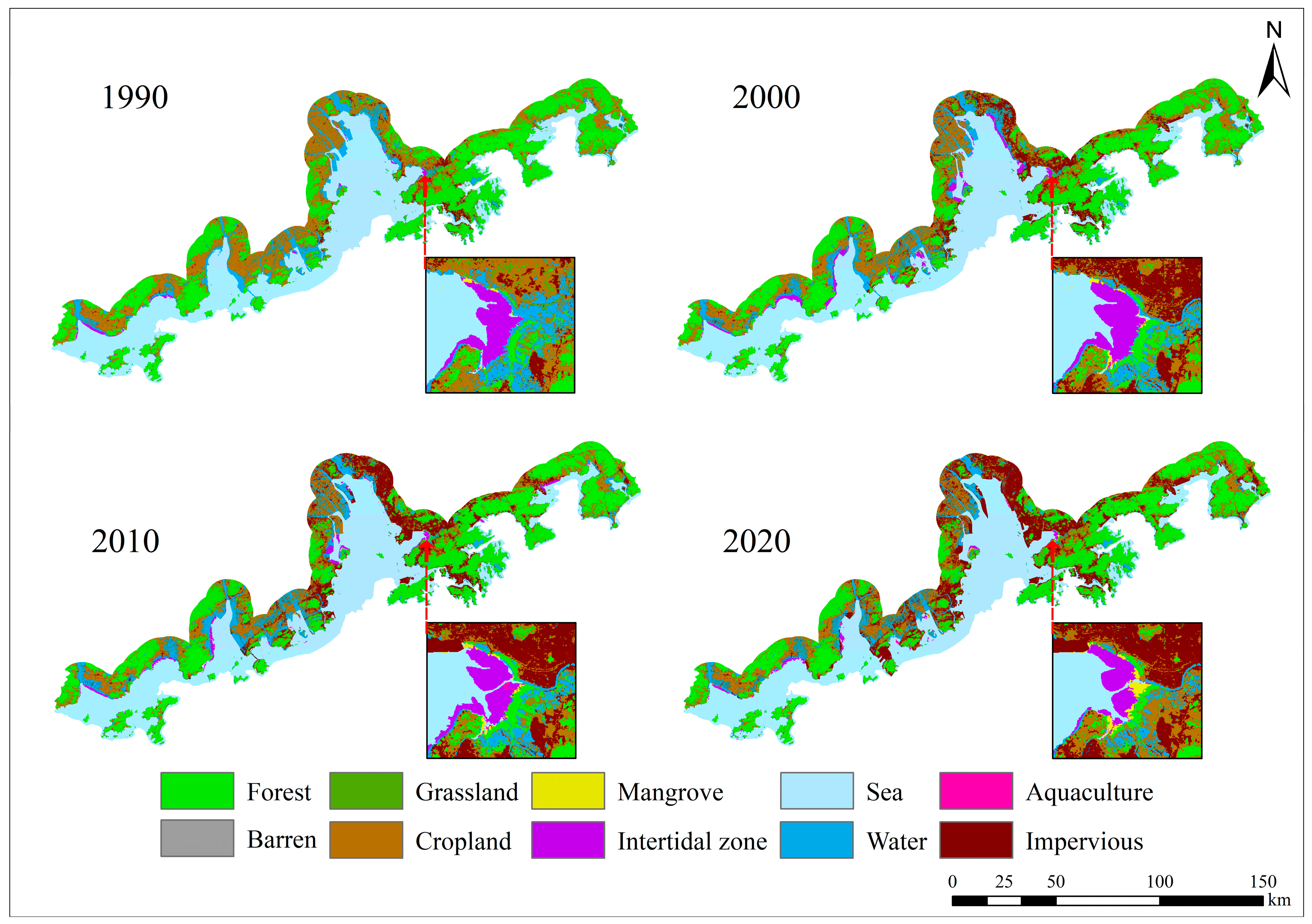
Based on statistical analysis of land cover proportions across four temporal scales (1990, 2000, 2010, and 2020), cultivated land, forestland, impervious surfaces, and water bodies exhibited notable dynamics. Cultivated land accounted for 20.77% in 1990 but declined steadily to a minimum of 15.28% by 2010, followed by a partial recovery to 16.46% in 2020, reflecting an overall U-shaped trajectory. Forestland reached its peak coverage of 30.22% in 1990, fluctuated within a narrow range (28.17% in 2000, 28.71% in 2010), and stabilized at 27.21% in 2020, demonstrating relative stability with minor oscillations. Impervious surfaces, initially minimal at 1.99% in 1990, exhibited a consistent upward trend, surging to 12.96% by 2020. Water bodies displayed a contrasting pattern, peaking at 8.36% in 2010 before declining to 6.47% in 2020. These trends are visually summarized in Figure 2, which illustrates land cover configurations for the four reference years.
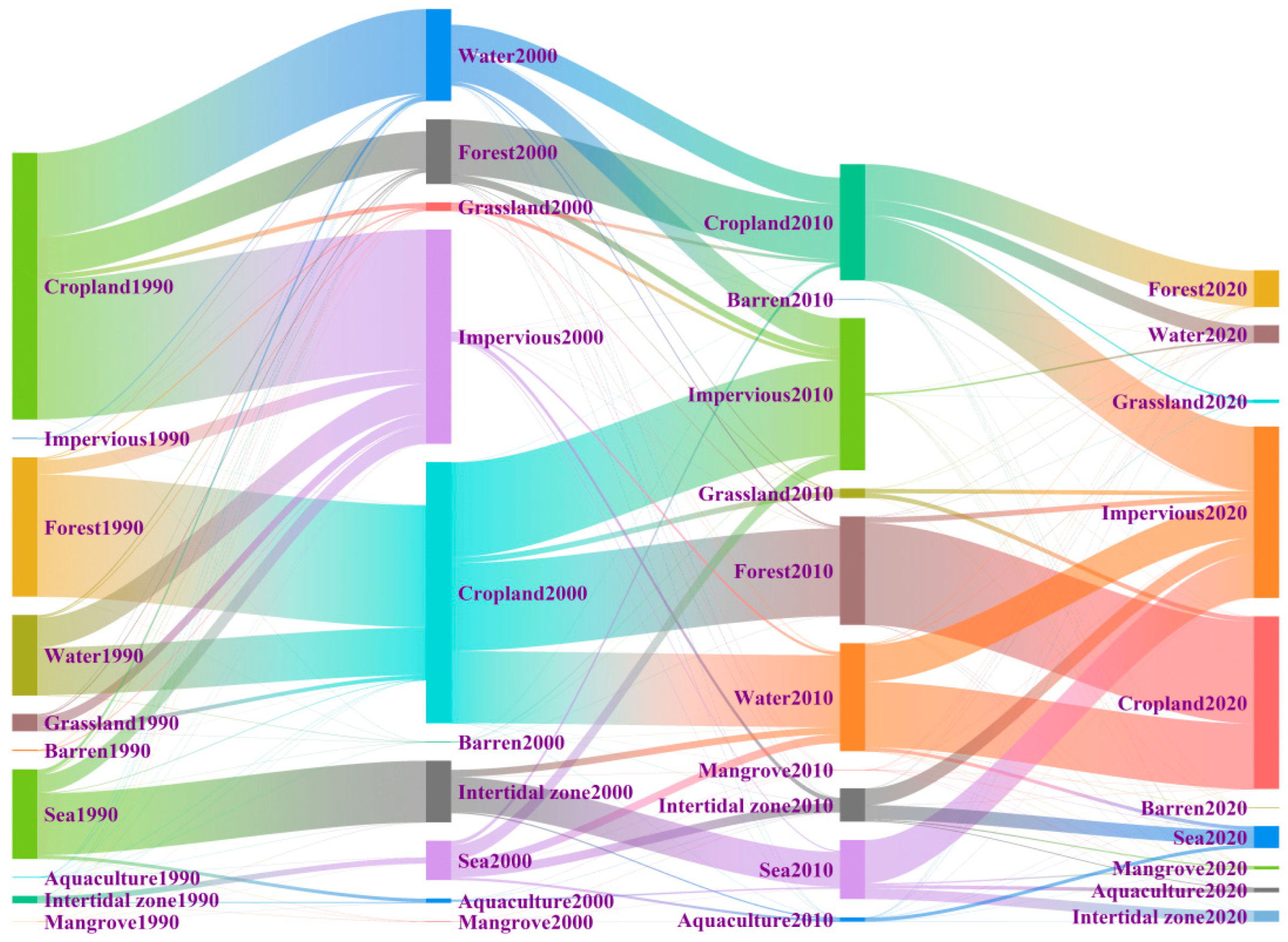
Over the three decades from 1990 to 2020, cultivated land exhibited the largest transfer area among all land use types. During the 1990–2000 period, cultivated land primarily transitioned into impervious surfaces and water bodies, while partial conversions occurred from forestland and water bodies to cultivated land; additionally, significant portions of coastal waters were converted into mudflats, and most land categories showed a tendency to shift toward impervious surfaces. In the 2000–2010 period, cultivated land remained the most transferred land type, mainly shifting to impervious surfaces, forestland, and water bodies, with a substantial area of forestland reverting to cultivated land during this interval. By the 2010–2020 period, transfer areas for cultivated land, forestland, and water bodies decreased but remained significant; notably, the proportion of forestland and water bodies converting to cultivated land increased by 2020. Concurrently, impervious surfaces continued to expand, with their primary sources of transfer being cultivated land, water bodies, and coastal waters (Figure 3).

3.2. Ecosystem Service Value Assessment

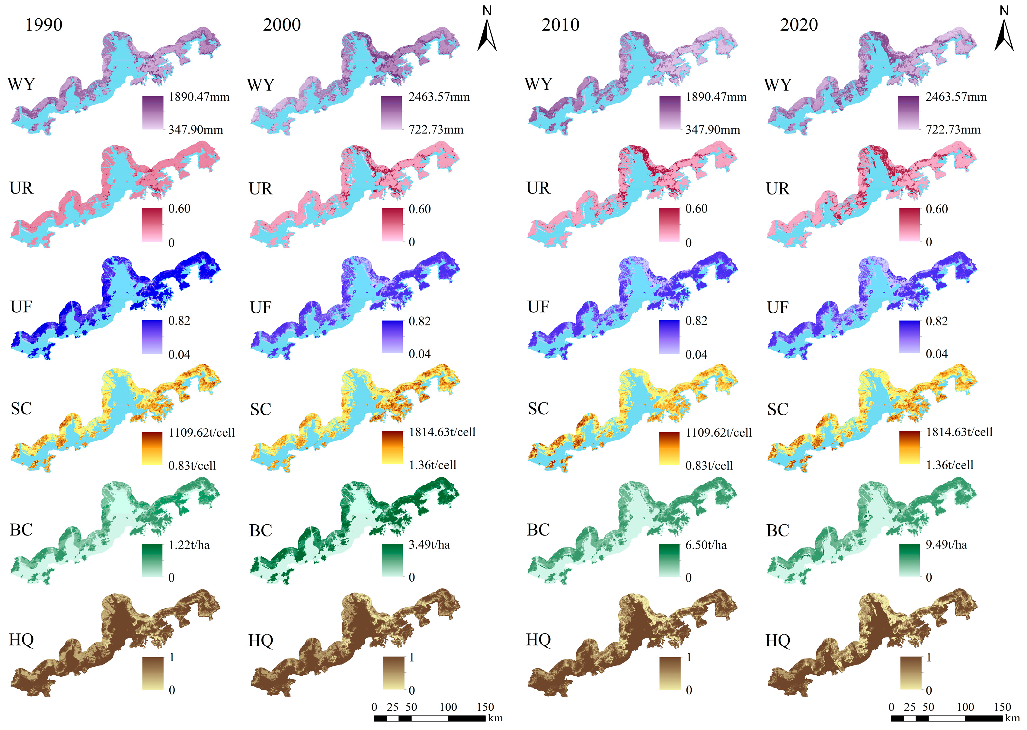
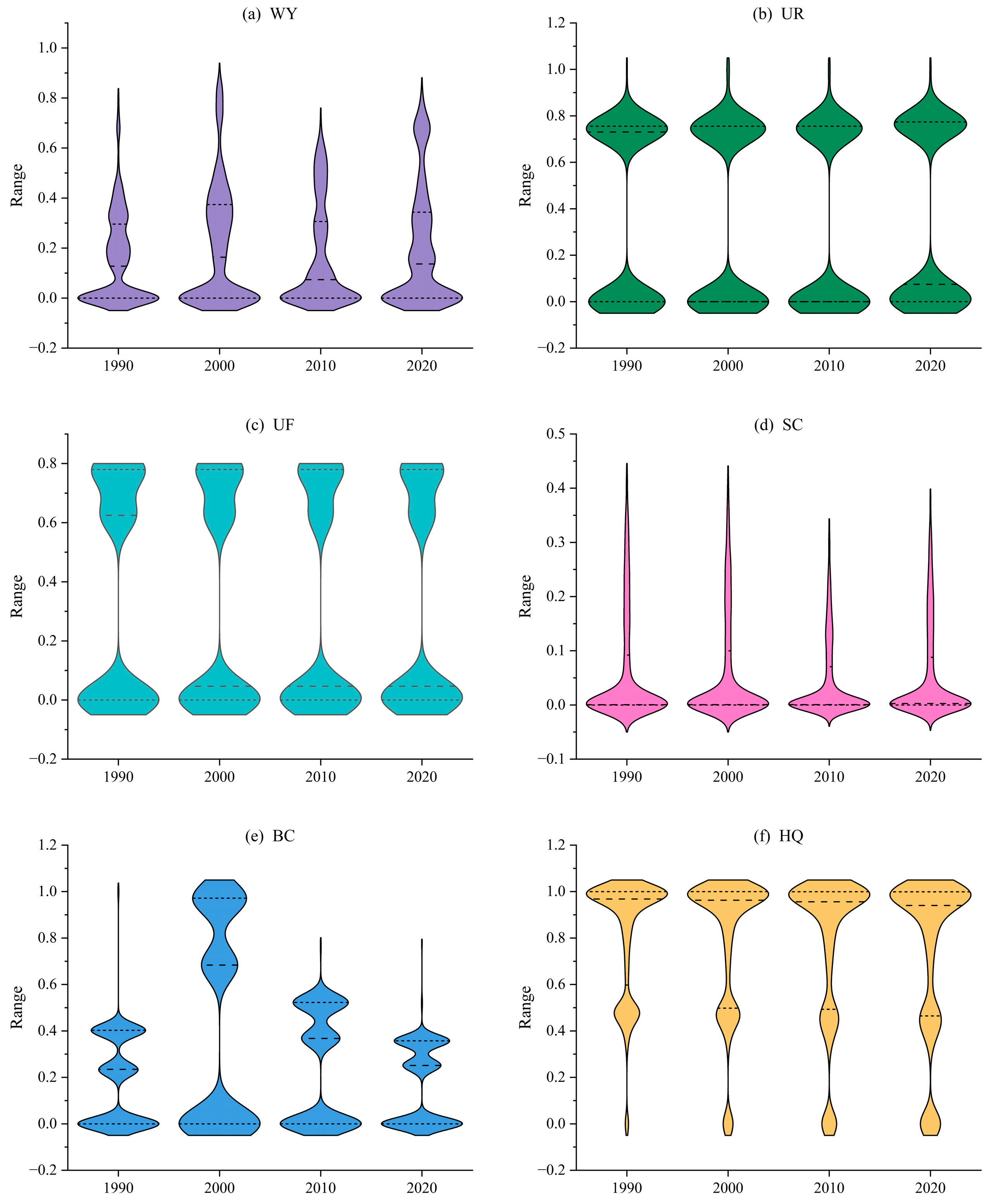
The spatial distribution maps (Figure 4) and service value statistics (Figure 5) of ecosystem services in the study area are presented as follows: Between 1990 and 2020, annual water yield exhibited significant fluctuations, with the lowest value of 799.19 mm in 1990, peaking at 1399.03 mm in 2000 before gradually declining to 950.29 mm by 2020; spatially, high values were concentrated in the central Pearl River Delta region, while lower values were observed in the eastern and western flanks. The urban rainwater retention rate reached its maximum of 100% across all four years, with the lowest value of 35.5% in 2020—low-retention areas were closely associated with urban construction expansion, concentrated in the central Pearl River Delta, whereas high-retention areas were distributed in the eastern and western regions, with stable data dispersion and minimal interannual variability. For flood risk mitigation capacity, the runoff interception value continuously declined, with the average decreasing from 0.56 in 1990 to 0.46 in 2020; low-value zones expanded from central and western regions to the eastern and western flanks, and ecosystem service values were predominantly concentrated in the ranges of 0–0.2 and 0.5–0.8, with the highest proportion of high values in 1990 and the lowest in 2010.
Soil retention service first increased then decreased, rising from 133.84 tons/grid cell in 1990 to a peak of 208.78 tons/grid cell in 2000 before dropping to 131.34 tons/grid cell by 2020; spatially, values in central and western regions were lower than those in the east, with minor interannual fluctuations, the highest proportion of high values in 1990, and the lowest in 2010. Coastal blue carbon storage continuously increased, with CO2 storage rising from 1.22 tons/hectare in 1990 to 9.49. tons/hectare in 2020, driven notably by tidal flats and mangroves; the spatial distribution of carbon storage expanded significantly between 1990–2000 but stabilized thereafter, though with fluctuations in dispersion. Habitat quality mean values declined steadily from 0.82 in 1990 to 0.73 in 2020, with lower values in central regions (sharpest decline in the central area) and higher values maintained in the east; data were predominantly distributed in the 0.4–1.0 range, with maximum values stable near 1.0 and minimal interannual dispersion.

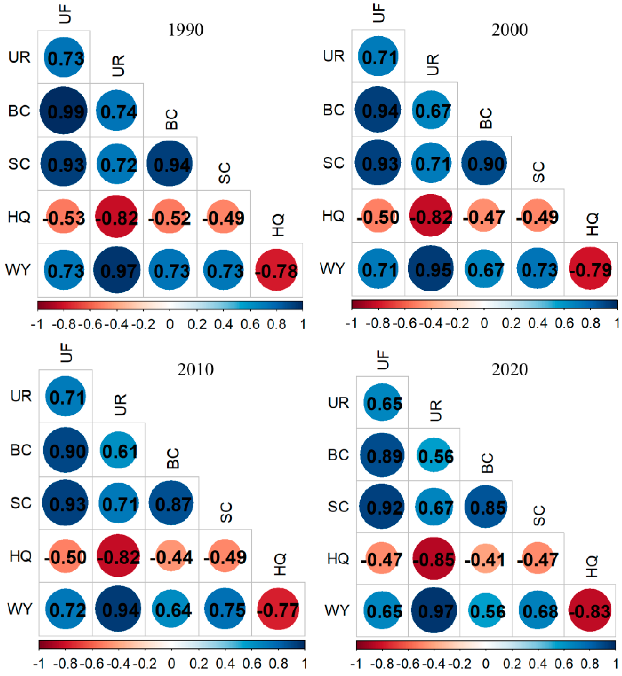
3.3. Trade-Offs and Synergies Among Ecosystem Services

During the period from 1990 to 2020, the Spearman correlation coefficients among the six ecosystem services revealed ten synergistic relationships among UF, UR, BC, SC, and WY, and five trade-off relationships involving HQ and other ecosystem services (Figure 6). All pairwise correlations among ecosystem services were statistically significant (p < 0.001). The trade-offs and synergies of ecosystem services were consistent across the four time points. In 1990, the strongest synergy was observed between UF and BC, with a correlation coefficient of 0.99. In 2000, 2010, and 2020, the strongest synergy appeared between UR and WY, with correlation coefficients of 0.95, 0.94, and 0.97, respectively. For all four years, the strongest trade-off relationship was observed between HQ and UR, with correlation coefficients of −0.82 from 1990 to 2010, and −0.85 in 2020.Over the thirty-year period from 1990 to 2020, synergies among UR and UF, BC and UF, BC and UR, SC and UF, SC and UR, SC and BC, as well as WY and BC gradually weakened. Meanwhile, trade-offs between HQ and UF, HQ and BC, and HQ and SC also showed a decreasing trend.

3.4. Spatial Distribution Patterns of Ecosystem Services

The results of the global spatial autocorrelation analysis for the six ecosystem services are presented in Table 4. For all four study years, the Moran’s I values for the six ecosystem services were positive and greater than 0.75 (p < 0.001), indicating a strong and statistically significant positive spatial autocorrelation. This suggests that ecosystem services with similar attributes tend to be spatially clustered.
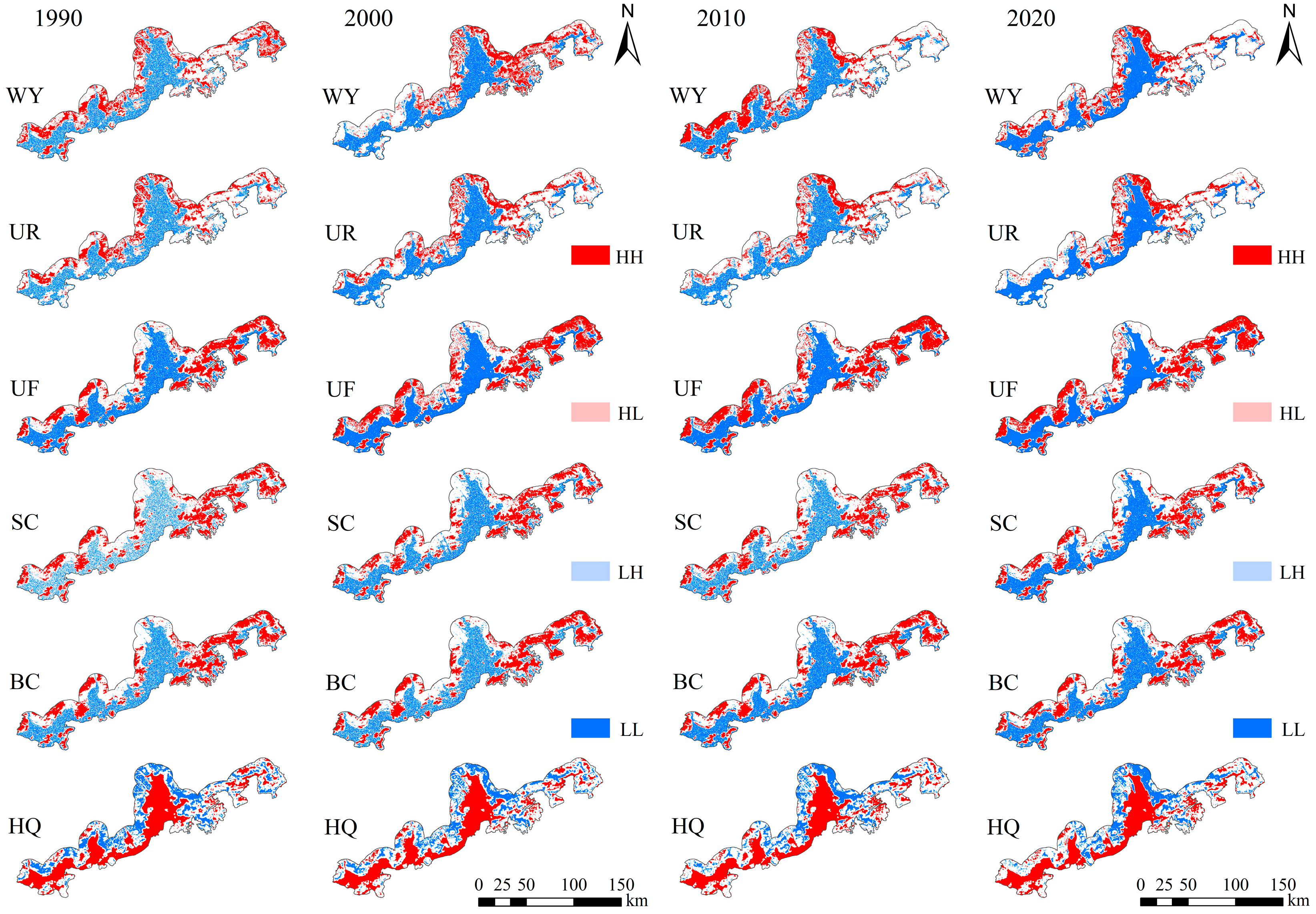
The results of the clustering and outlier analysis (Figure 7) reflect local spatial autocorrelation. Across the four study years, spatial differences in the clustering patterns of the six ecosystem services remained relatively stable, although the degree of clustering changed over time. Habitat quality (HQ) generally exhibited a low-low (LL) clustering pattern in terrestrial areas and a high-high (HH) clustering pattern in marine areas, indicating higher habitat quality in marine environments and a tendency toward high-value agglomeration. In contrast, water yield (WY), urban runoff regulation (UR), urban flood regulation (UF), soil conservation (SC), and blue carbon (BC) displayed HH clustering patterns in terrestrial zones and LL patterns in marine zones. The terrestrial clustering of HQ was primarily concentrated in the central Pearl River Estuary, with particularly pronounced clustering in the eastern part, while the degree of clustering in the western part gradually weakened. Over time, the LL clustering of HQ in terrestrial areas intensified. WY and UR exhibited similar clustering patterns on land, mainly in the eastern Pearl River Estuary and the western part of the study area. The clustering in the western region gradually weakened, while clustering in the eastern estuary increased. UF, SC, and BC also shared similar terrestrial clustering patterns, predominantly in the eastern and western regions, with UF showing the most evident clustering. Over the 30-year period, the spatial and temporal variation in clustering for these three services remained limited. All six ecosystem services showed positive spatial autocorrelation, with most areas exhibiting HH or LL clustering patterns. HL and LH clusters were rare, indicating that outlier patterns (high-value surrounded by low-value, or vice versa) were spatially limited and often associated with transitional or fragmented landscapes, such as urban parks or reclaimed wetlands.

3.5. Selection of Driving Factors and Impact Mechanisms

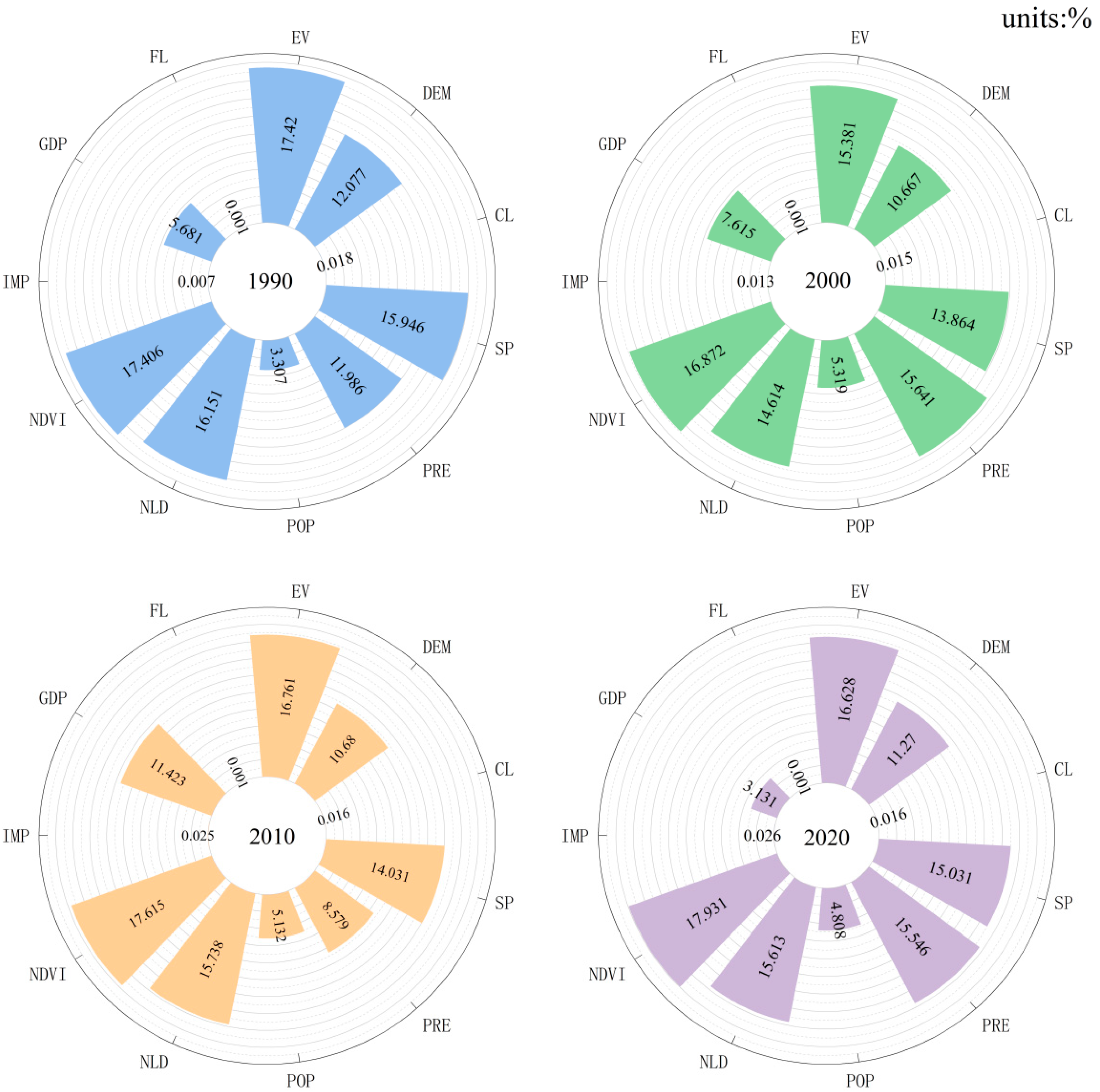
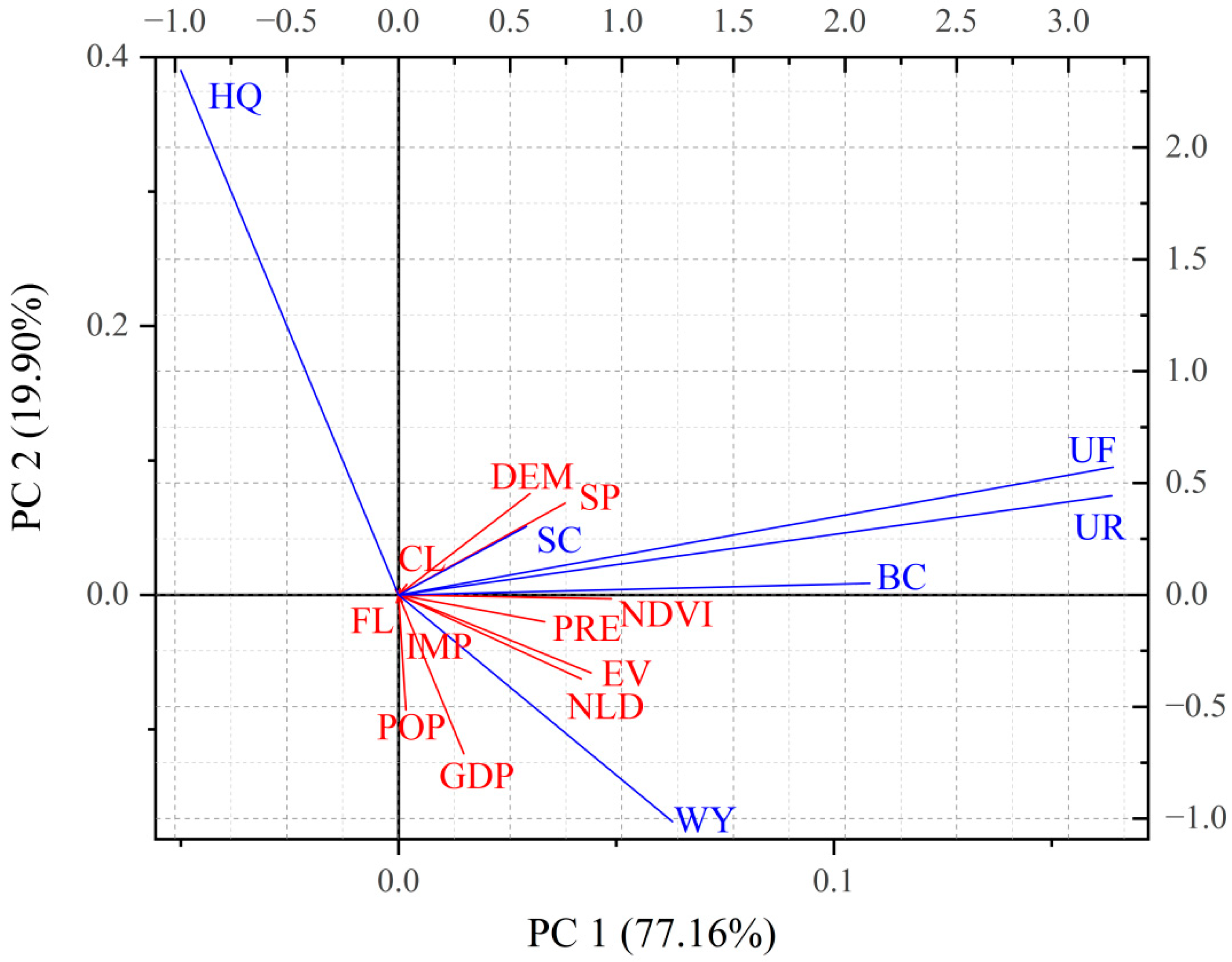
Redundancy analysis (RDA) was used to determine the contribution of various driving factors to ecosystem service values across the four study years (Figure 8), along with the RDA ordination results (Figure 9). In 1990, the explanatory variables with the highest influence were evapotranspiration (EV), normalized difference vegetation index (NDVI), and nighttime light index (NLD), each contributing more than 15% to ecosystem service values. In 2000, NDVI, precipitation (PRE), and EV each contributed more than 15%. In both 2010 and 2020, NDVI, EV, and NLD consistently ranked among the top three influential factors, all exceeding the 15% threshold. In contrast, forest land (FL), cultivated land (CL), and impervious surface percentage (IMP) had relatively low influence. However, the influence of IMP was more pronounced than that of FL and CL, increasing steadily from 0.007% in 1990 to 0.026% in 2020. Therefore, NDVI and EV (natural factors), IMP (land use change factor), and NLD (socio-economic factor) are identified as the primary drivers of ecosystem service values.
Mechanistic interpretation of coefficient patterns: (1) Night-time light index (NLD) shows region- and time-dependent sign changes because early urbanization increases infrastructure that may concentrate water services (e.g., water yield from engineered sources) in built areas (leading to transient positive correlations), whereas later intensification and impervious expansion reduce natural service provision and thus produce a negative association in densely lit urban cores. (2) The effect of impervious surface proportion (IMP) weakens over time in many areas likely because early land-cover change produced the largest marginal impacts on hydrological and habitat processes; as urban surfaces stabilize and mitigation measures (e.g., stormwater management, constructed wetlands) are introduced, incremental IMP increases produce smaller marginal changes in modeled ES. (3) NDVI exerts contrasting effects because vegetation enhances regulating/supporting services (UF, UR, SC, BC, HQ) through evapotranspiration moderation, soil protection and carbon uptake, but reduces modeled annual water yield (WY) due to increased transpiration losses. Spatially, NDVI’s positive effect on BC is strongest in mangrove and tidal flat zones where vegetated coastal habitats sequester disproportionate carbon per unit area.
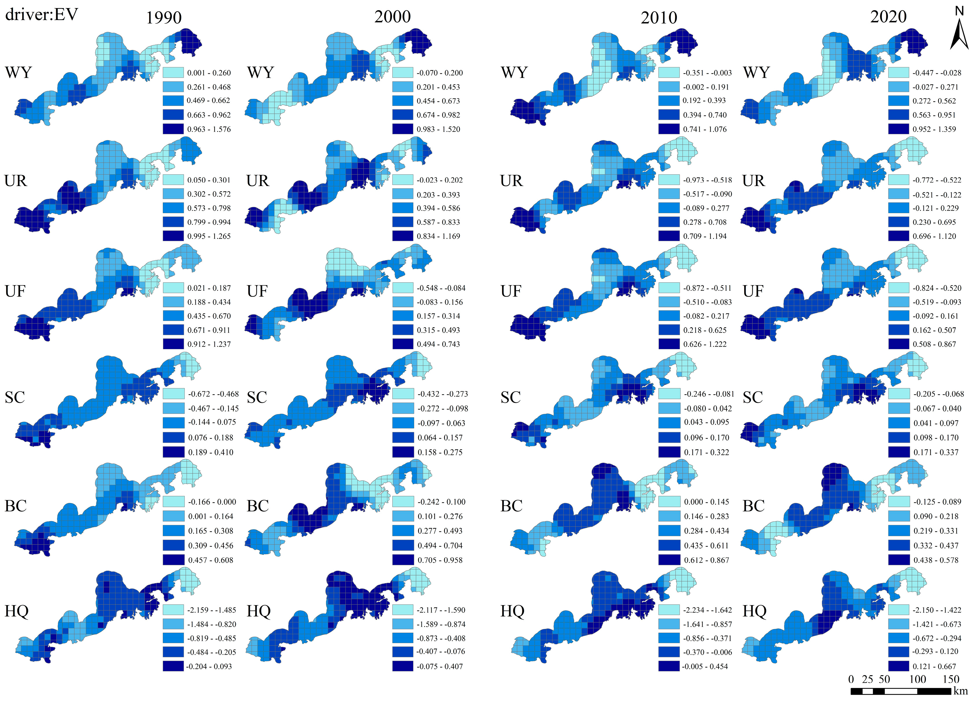
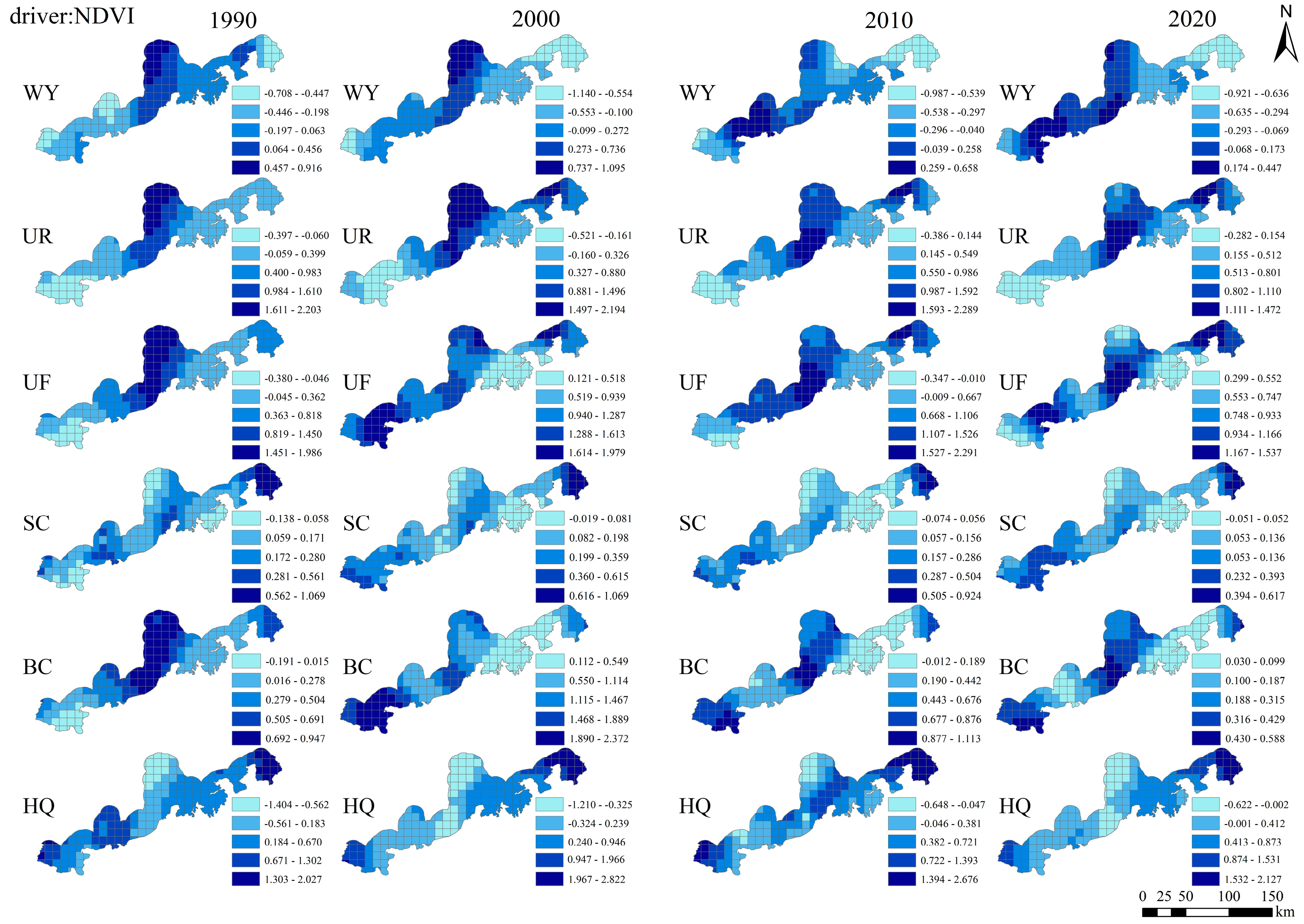
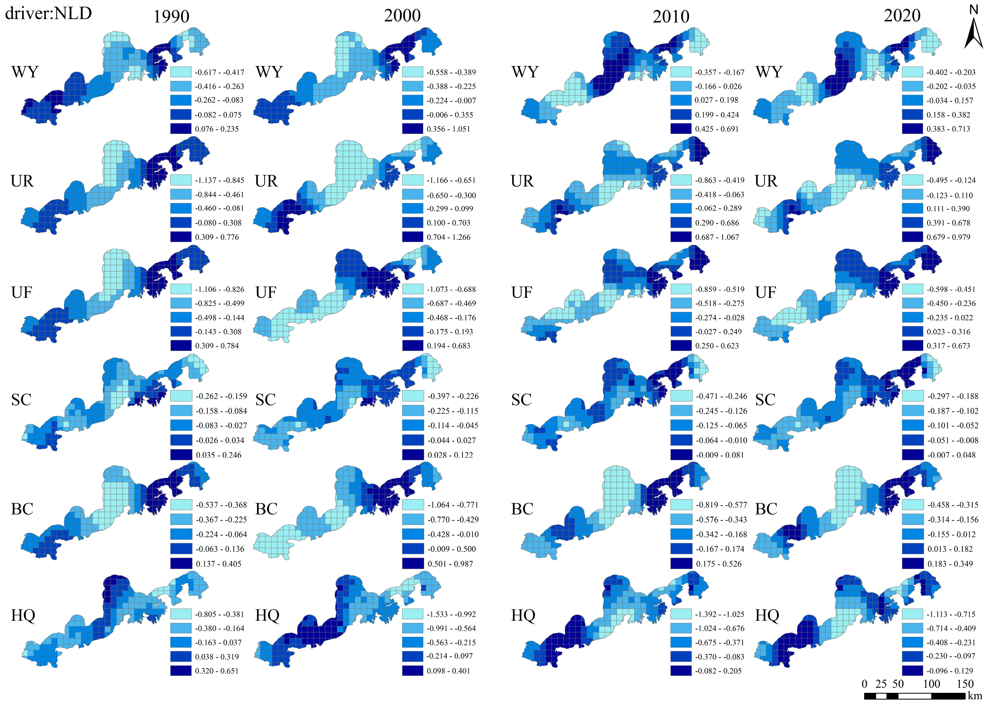
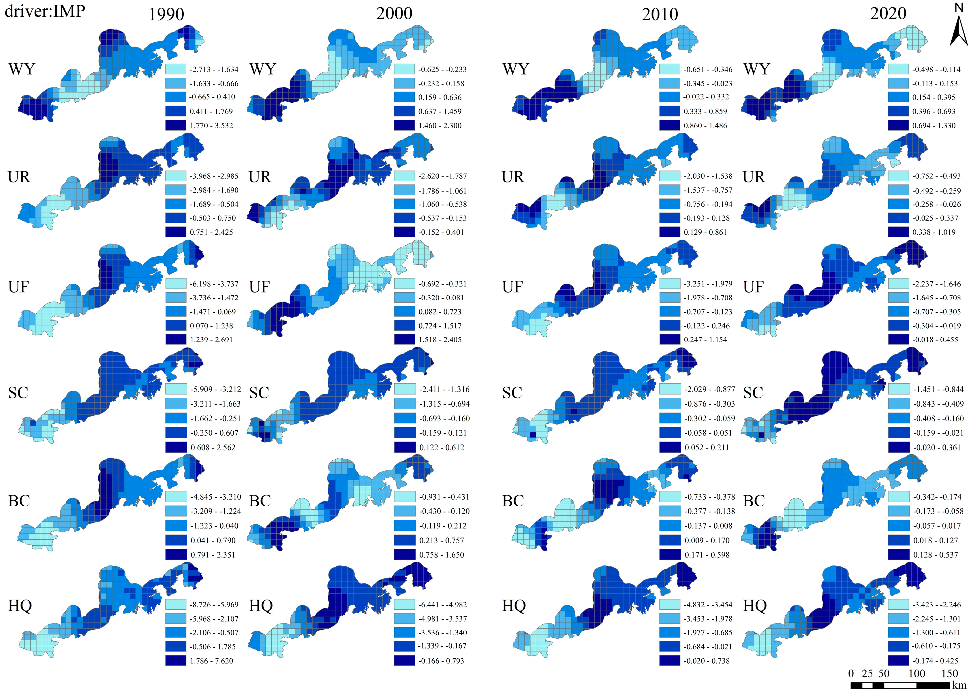
To further explore the mechanisms by which the four main drivers—NDVI, EV, NLD, and IMP—influence ecosystem services, GTWR regression analysis was conducted. The spatial distribution of GTWR coefficients for each driver is presented in Figure A1, Figure A2, Figure A3 and Figure A4 in the Appendix A. For WY, NDVI was positively correlated in the central-western region during 1990–2000 and negatively correlated elsewhere; the positively correlated region shifted westward during 2010–2020. EV was mostly positively correlated in the early years, with a shift to negative correlation in the Pearl River Estuary and its western surroundings in later years. NLD was mainly negatively correlated in the early years but became positively correlated in the estuary and western areas later. IMP showed positive correlation in the north and at the eastern and western ends in earlier years, turning negative in the western estuary and eastern region in later years.
For UR, NDVI was negatively correlated in the west and positively correlated in the central-east during the early years, with the negatively correlated area shrinking over time. EV was positively correlated early on, shifting to negative in the estuary and eastern regions. NLD remained negatively correlated in the estuary and its west throughout, while being positively correlated elsewhere. IMP showed negative correlation except in the western estuary and western end, with its influence weakening over time. For UF, NDVI was positively correlated in 2000 and 2020, but negatively correlated in the western region in 1990 and 2010. EV was positively correlated in 1990, while becoming negatively correlated in central and eastern regions in later years, and positively correlated in the western estuary. NLD was negatively correlated in the western estuary and positively correlated in the east. IMP was positively correlated in the central region in earlier years, turning mostly negative later. For SC, the effects of NDVI and EV showed no distinct spatial or temporal patterns, with each showing positive or negative correlations in specific regions. NLD and IMP were generally negatively correlated across the study area, and the strength of correlation decreased over time. For BC, NDVI was consistently positively correlated, with stronger effects in the central and western regions—highest in 2000 and lowest in 2020. EV was positively correlated in 2010, with some negative correlations in the central-eastern region during other years. NLD showed negative correlations in the central-west and positive correlations in the east. IMP displayed varying correlations across the east, west, and central parts of the study area in different years. For HQ, NDVI’s spatial variation remained relatively stable, showing positive correlations in the east and west, and negative in the central-west. EV was mostly negatively correlated, with stronger effects in the eastern region. NLD was negatively correlated in the east and west and positively in the central region in the early years, but predominantly negative in later years. IMP was negatively correlated in the west and positively in the east early on, shifting to mostly negative correlations in later years.

4. Discussion

4.1. Land Use Change and Ecosystem Service Value

Based on the land use transition matrix, we found that the most notable changes from 1990 to 2020 occurred in cultivated land, forest land, impervious surfaces, and water bodies, which is consistent with the findings of [41]. Among these, cultivated land experienced the largest change, showing a continuous decline from 1990 until a slight rebound by 2020. The early-stage decrease in cultivated land is closely related to the substantial encroachment driven by urban expansion to meet the economic development demands of the Guangdong-Hong Kong-Macao Greater Bay Area, resulting in drastic land use changes [42]. The later-stage rebound was attributed to a series of policies aimed at protecting cultivated land and promoting afforestation, which helped to curb the loss of arable land. Although the change in forest area was relatively small, it exhibited an overall declining trend under the dual influence of land development and ecological protection policies. The most rapid increase over the thirty-year period was observed in impervious surfaces, which aligns with the findings of [43]. This reflects the extensive development of construction land and transportation infrastructure in the Greater Bay Area alongside accelerated urbanization [44], which has altered the characteristics of the underlying surface. Water bodies showed a trend of first increasing and then decreasing, reaching the lowest level in 2020. The initial increase was driven by the development of aquaculture, while the subsequent decline resulted from large-scale land reclamation projects undertaken to meet urban land demands, leading to reductions in both inland and marine water areas.
Based on the InVEST model assessment of six ecosystem services, we found that the annual water yield was similar to that reported by [45], though variations in study area size may have introduced some degree of error and led to significant interannual fluctuations [46]. Habitat quality was consistent in both results and trends with [41]. Differences in soil retention arose due to variations in the selection of calculation factors and construction of biophysical tables, resulting in deviations from [41], though within an acceptable range. The coastal blue carbon storage results differed slightly and were higher than typical terrestrial carbon storage estimates. This discrepancy may be due to the inclusion of coastal land use types in the input data. The unit area carbon sequestration capacity of coastal vegetation ecosystems is 3–5 times that of terrestrial forests [47]. Furthermore, aquaculture areas, mangroves, and mudflats are natural carbon sinks with strong carbon sequestration capabilities [48], capable of absorbing and storing substantial amounts of CO2, leading to higher estimates in our calculations—consistent with the objectives of this study. Changes in ecosystem service values over time are influenced not only by natural factors but also by socioeconomic drivers and interactions with the surrounding environment. Therefore, it is essential to incorporate ecosystem services into coastal planning considerations to enhance the realization of positive value [49].
Compared to other InVEST-based coastal studies (e.g., Liu et al., 2022 in the Pearl River Delta [41]; Ma et al., 2019 in the Yellow River Delta [1]), our study incorporated marine-specific land classes and blue carbon pools, leading to higher carbon storage estimates. Our water yield values aligned with [45], but habitat quality trends differed slightly due to our inclusion of marine habitat suitability. These differences underscore the importance of region-specific parameterization and classification in coastal ES modeling.
Based on the analysis of land use transitions, we conclude that land use change has a significant impact on ecosystem service values. During the expansion and development of the Greater Bay Area, cultivated and forest lands declined, while impervious surface areas increased markedly. As the underlying surface was altered, surface runoff and interception were affected, reducing ecosystem service values and increasing the risk of urban flooding and the economic burden of stormwater management [50]. At the same time, the rise in surface runoff has accelerated soil erosion, weakening the ecosystem’s regulation services such as flood control and soil retention. Continuous human activities have also led to environmental degradation, habitat destruction, and pollution, further contributing to the annual decline in habitat quality. On a global scale, land cover changes likewise negatively affect ecosystem service values [51]. In terms of coastal blue carbon, the protection and restoration of mangrove ecosystems [52] and the enhanced value of wetland ecosystem services [53] have improved the carbon storage capacity of blue carbon ecosystems, resulting in a continuous increase in blue carbon stocks.

4.2. Trade-Offs, Synergies, and Driving Factor Analysis

Among the results of trade-off and synergy analysis, ten synergistic relationships were consistent with those reported by [54], though different trade-off patterns were observed in ecosystem service pairs involving habitat quality (HQ). Considering that this study included marine areas in the calculation of ecosystem services, the Greater Bay Area, while enhancing coastal blue carbon and increasing terrestrial regulating and supporting services, often did so at the cost of degrading parts of the marine environment. The intensified land use has exacerbated trade-offs between services [55], disrupting ecological balance in marine areas and thereby exhibiting trade-off relationships. This provides new insights into the rational management and spatial planning of land in the Greater Bay Area. Furthermore, our study found stronger synergies among ecosystem service pairs, such as urban runoff (UR) and water yield (WY), which showed the strongest synergistic relationship. Increased rainwater retention enhanced both surface and groundwater availability, thereby improving the water retention capacity of the ecosystem. At the same time, water availability supports vegetation growth, and good vegetation cover and soil conditions facilitate rainwater infiltration and storage, enhancing urban rainwater retention capacity. These findings indicate that different components of ecosystems influence and constrain each other to achieve a supply-demand balance [56,57].
Results from the spatial autocorrelation analysis revealed significant positive spatial correlations in ecosystem services, with a tendency for high-high and low-low clustering patterns. We found significant spatial autocorrelation in ecosystem service values, consistent with findings from [58]. This suggests that ecosystem service levels in adjacent regions are highly similar, and the status of ecosystem services in one area tends to exert a similar influence on neighboring regions. Spatial visualization of the autocorrelation analysis showed that high-high clustering areas usually possess strong ecological foundations and abundant natural resources, with high values in services such as water conservation and biodiversity maintenance. Conversely, low-low clustering areas are often subject to intense human disturbance and ecological degradation or have poor natural endowments, resulting in damaged ecosystem structures, degraded functions, and reduced ecosystem service values.
Spatial autocorrelation partly arises from the choice of spatially continuous indicators (e.g., NDVI, evapotranspiration) and the grid resolution. To reduce or explicitly account for autocorrelation in future work we recommend (i) aggregating outputs to coarser reporting units (e.g., 1-km cells or watersheds) to reduce local spatial noise, (ii) using spatial regression methods (spatial lag/error models, GWR/GTWR) that explicitly model spatial dependence, and (iii) detrending variable surfaces (removing large-scale gradients) before local autocorrelation diagnostics. In this study, GTWR was used to capture localised driver effects while the Moran’s I and LISA maps identify clustering patterns for targeted management.
Analysis of driving factors indicated that among natural variables, the Normalized Difference Vegetation Index (NDVI) and evapotranspiration (EV); among land use variables, the proportion of impervious surfaces (IMP); and among socio-economic variables, the nighttime light index (NLD), were the primary factors influencing ecosystem service values. The findings of [23,38] also highlighted the significant roles of NDVI and IMP in shaping ecosystem service values. NDVI was a positive driving factor in most regions for UR, UF, SC, BC, and HQ, indicating its positive effect on ecosystem service enhancement. However, WY showed a generally negative correlation with NDVI, as vegetation tends to intercept precipitation and reduce water retention through transpiration. EV had relatively limited spatial differentiation impacts on most ecosystem services over the thirty-year period but exhibited varying degrees of influence. EV was mainly positively correlated with BC and negatively correlated with HQ, while the direction of its influence on other services displayed spatial heterogeneity. The influence of NLD was predominantly negative, with considerable spatial variation over time. Research by [59] revealed that NLD exhibits a threshold effect under negative correlation, indicating that human activities can alter both the spatial distribution and value of ecosystem services. IMP showed mainly negative correlations with HQ, SC, and UR, and its impact weakened over time. Economic development in the Greater Bay Area led to extensive land use expansion and increased ecological vulnerability [60]. In addition, land reclamation and similar activities significantly increased impervious surface coverage, damaging the original ecological environment and negatively impacting ecosystem services such as habitat quality, soil retention, and hydrological regulation [46,61]. Analyzing the driving factors of ecosystem services not only clarifies the relationships between services and their influencing factors but also helps predict future trends in ecosystem service changes. This provides critical support for ecological protection, land use planning, and the sustainable management of natural resources and the environment.
The observed spatio-temporal sign changes in NLD and the temporal attenuation of IMP effects reflect socio-ecological dynamics: NLD may show an initial positive correlation with some water-related services in peri-urban zones where infrastructure and irrigation amplify local water availability, then switch to negative correlations in dense urban cores where anthropogenic pressures reduce ecosystem functionality. This aligns with threshold effects reported in urbanization studies [59]. The weakening impact of IMP over time can be explained by (a) saturation effects—early conversion of permeable to impermeable surfaces produces the largest hydrological shifts—and (b) adaptive management such as SUDS/green infrastructure implementation in later decades. The NDVI paradox (positive for most regulating/supporting services but negative for WY) is consistent with ecohydrological theory (Budyko-type processes): increasing vegetation cover enhances infiltration, reduces erosion, and increases carbon uptake but raises evapotranspiration, reducing net water yield available at grid scale [27].

4.3. Research Significance and Limitations

This study presents several innovative aspects: (1) The study area encompasses the coastal zone of the GBA, incorporating marine areas into the assessment of ecosystem services, thereby acknowledging the service value of the marine ecosystem; (2) The inclusion of land use types such as mangroves, mudflats, and aquaculture enhances the regional applicability of the findings and broadens the scope of land use types considered in ecosystem service valuation; (3) The carbon storage calculations in this study differ from those in other studies by focusing on the ecosystem service value of coastal blue carbon; (4) The study quantifies ecosystem service values related to urban rainwater retention and flood risk mitigation, contributing to an improved understanding of urban resilience to extreme weather events and enriching the typology of ecosystem services.
Research on ecosystem services in coastal zones holds significant relevance for the Greater Bay Area. First, it provides a methodological reference for the assessment of ecosystem service values in coastal areas. Second, by clarifying the values, trade-offs, synergies, and driving forces of coastal ecosystem services, this study enhances our understanding of the functions and dynamics of these services. Furthermore, by analyzing spatial heterogeneity, it identifies inter-city differences in ecosystem service provision [53], thereby offering a scientific foundation for regional management, land use planning, and industrial spatial layout. It also emphasizes the importance of ecosystem services in supporting ecological protection, biodiversity conservation, and the coordinated development of ecological, economic, and social systems. Current research on coastal ecosystem services has increasingly adopted various methods to detect spatiotemporal changes in coastal land use [62]. Based on the economic valuation of ecosystem services [63], researchers have explored strategies for maintaining the balance between supply and demand of ecosystem services and ecosystem protection through identifying ecosystem service bundles, constructing ecological corridors, and other approaches [64], thus providing scientific support for realizing ecosystem service values in coastal zones [65] and enhancing human well-being [66].
The quantified ecosystem service values revealed in this study provide direct guidance for coastal spatial planning and ecological management in the Guangdong–Hong Kong–Macao Greater Bay Area. The continuous decline in habitat quality and flood regulation capacity highlights the urgent need to strictly control the expansion of impervious surfaces and to optimize urban land-use structures. Priority protection zones should be delineated for areas with high ecosystem service values, particularly mangroves, tidal flats, and coastal wetlands, given their outstanding contributions to blue carbon sequestration, flood mitigation, and biodiversity conservation. Furthermore, the significant increase in coastal blue carbon storage supports the integration of blue carbon ecosystems into regional carbon neutrality strategies and emerging carbon trading mechanisms, thereby enhancing the economic incentives for coastal ecological restoration. From a management perspective, ecosystem service values should be embedded into territorial spatial planning, ecological compensation schemes, and disaster risk reduction policies to balance rapid urbanization with long-term ecological security and sustainable development.
This study also has several limitations. First, the quantification of ecosystem services relies solely on the InVEST model, which may lead to inaccuracies due to the simplification of complex ecosystem processes inherent in the model [67]. Second, some model parameters were set according to relevant local literature, which were lack of field data and sensitive analysis. Future research should aim to address these limitations by refining the methodological framework.

5. Conclusions

Taking the coastal zone of the Guangdong-Hong Kong-Macao Greater Bay Area as the study area, this study incorporated marine areas into the assessment and refined the land use classification by including mangroves, mudflats, and aquaculture. Land use changes were analyzed for the years 1990, 2000, 2010, and 2020. Six ecosystem services—water yield (WY), urban runoff regulation (UR), urban flood regulation (UF), soil conservation (SC), blue carbon (BC), and habitat quality (HQ)—were quantified and their spatial distribution characteristics examined. The trade-offs and synergies among ecosystem services were analyzed using Spearman correlation coefficients. Driving factors of ecosystem services were identified through RDA and the GTWR model. The following conclusions were drawn:
(1)
Cropland, forest, impervious surfaces, and water bodies were the land use types with the greatest changes over the past three decades in the Greater Bay Area;
(2)
Most of the relationships among the six ecosystem services were synergistic, although these synergies tended to weaken over time. Habitat quality exhibited trade-off relationships with the other five services;
(3)
Among the driving factors, the Normalized Difference Vegetation Index (NDVI) and evapotranspiration (EV) from the natural domain, the proportion of impervious surfaces (IMP) from land use change, and the nighttime light index (NLD) from the socio-economic domain were identified as the primary drivers influencing coastal ecosystem services. These factors had spatially and temporally differentiated effects. NDVI had a generally positive influence and contributed positively to the evolution of ecosystem services, while NLD generally had a negative effect.
The study provides a valuable reference for land use and ecological planning in coastal zones and contributes to the sustainable development of the human-ocean coupled ecosystem.

Author Contributions

Conceptualization, Z.W.; Methodology, Z.W.; Software, C.L.; Formal analysis, C.L.; Investigation, C.Y.; Resources, M.X.; Data curation, X.S.; Writing—original draft, C.L.; Writing—review & editing, Z.W., X.S. and C.Y.; Project administration, M.X. All authors have read and agreed to the published version of the manuscript.

Funding

This study was supported by National Natural Science Foundation of China (Project NO.: 42207530) and Fundamental Research Funds for the Central Universities (Project NO.: 292022004).

Data Availability Statement

The data presented in this study are available on request from the corresponding author.

Conflicts of Interest

The authors declare no conflict of interest.

Appendix A

Figure A1. The spatial distribution of GTWR coefficients of NDVI.
Water 17 03566 g0a1
Figure A2. The spatial distribution of GTWR coefficients of EV.
Water 17 03566 g0a2
Figure A3. The spatial distribution of GTWR coefficients of NLD.
Water 17 03566 g0a3
Figure A4. The spatial distribution of GTWR coefficients of IMP.
Water 17 03566 g0a4

References and Note

  1. Ma, T.; Li, X.; Bai, J.; Ding, S.; Zhou, F.; Cui, B. Four decades’ dynamics of coastal blue carbon storage driven by land use/land cover transformation under natural and anthropogenic processes in the Yellow River Delta, China. Sci. Total. Environ. 2019, 655, 741–750. [Google Scholar] [CrossRef]
  2. Yang-Fan, L.; Zhi-Yuan, X.; Yi, Y.; Quan-Li, W.; Yi, L. Application of ecological restoration and planning based on resilience thinking in coastal areas. J. Nat. Resour. 2020, 35, 130–140. [Google Scholar] [CrossRef]
  3. Li, J.; Liu, Y.M.; Sun, H.; Huang, J.T.; Lu, J.F. Analysis of Blue Carbon in China’s Coastal Zone. Environ. Sci. Technol. 2019, 42, 207–216. [Google Scholar]
  4. Wang, F.; Lu, X.; Sanders, C.J.; Tang, J. Tidal wetland resilience to sea level rise increases their carbon sequestration capacity in United States. Nat. Commun. 2019, 10, 5434. [Google Scholar] [CrossRef] [PubMed]
  5. Bryan, B.A.; Nolan, M.; McKellar, L.; Connor, J.D.; Newth, D.; Harwood, T.; King, D.; Navarro, J.; Cai, Y.; Gao, L.; et al. Land-use and sustainability under intersecting global change and domestic policy scenarios: Trajectories for Australia to 2050. Glob. Environ. Chang. 2016, 38, 130–152. [Google Scholar] [CrossRef]
  6. van Zelst, V.T.M.; Dijkstra, J.T.; van Wesenbeeck, B.K.; Eilander, D.; Morris, E.P.; Winsemius, H.C.; Ward, P.J.; de Vries, M.B. Cutting the costs of coastal protection by integrating vegetation in flood defences. Nat. Commun. 2021, 12, 6533. [Google Scholar] [CrossRef] [PubMed]
  7. Costanza, R.; d’Arge, R.; De Groot, R.; Farber, S.; Grasso, M.; Hannon, B.; Limburg, K.; Naeem, S.; O’Neill, R.V.; Paruelo, J.; et al. The value of the world’s ecosystem services and natural capital. Nature 1997, 387, 253–260. [Google Scholar] [CrossRef]
  8. Costanza, R.; de Groot, R.; Braat, L.; Kubiszewski, I.; Fioramonti, L.; Sutton, P.; Farber, S.; Grasso, M. Twenty years of ecosystem services: How far have we come and how far do we still need to go? Ecosyst. Serv. 2017, 28, 1–16. [Google Scholar] [CrossRef]
  9. Plag, H.-P.; Jules-Plag, S. Sea-Level Rise and Coastal Ecosystems. Clim. Vulnerability 2013, 31, 163–184. [Google Scholar] [CrossRef]
  10. Millennium Ecosystem Assessment. Ecosystems and Human Well-Being: Biodiversity Synthesis; Island Press: Washington, DC, USA, 2005. [Google Scholar]
  11. Xie, G.D.; Zhang, C.X.; Zhang, L.M.; Chen, W.H.; Li, S.M. Improvement of the evaluation method for ecosystem service value based on per unit area. J. Nat. Resour. 2015, 30, 1243–1254. [Google Scholar]
  12. Fisher, B.; Turner, R.K.; Morling, P. Defining and classifying ecosystem services for decision making. Ecol. Econ. 2009, 68, 643–653. [Google Scholar] [CrossRef]
  13. Peng, J.; Wang, X.; Liu, Y.; Zhao, Y.; Xu, Z.; Zhao, M.; Qiu, S.; Wu, J. Urbanization impact on the supply-demand budget of ecosystem services: Decoupling analysis. Ecosyst. Serv. 2020, 44, 101139. [Google Scholar] [CrossRef]
  14. Schröter, M.; Koellner, T.; Alkemade, R.; Arnhold, S.; Bagstad, K.J.; Marques, A.; Frank, K.; Kastner, T.; Kissinger, M.; Liu, J.; et al. Interregional flows of ecosystem services: Concepts, typology and four cases. Ecosyst. Serv. 2018, 31, 231–241. [Google Scholar] [CrossRef]
  15. Chalkiadakis, C.; Drakou, E.G.; Kraak, M.-J. Ecosystem service flows: A systematic literature review of marine systems. Ecosyst. Serv. 2022, 54, 101412. [Google Scholar] [CrossRef]
  16. Howe, C.; Suich, H.; Vira, B.; Mace, G.M. Creating win-wins from trade-offs? Ecosystem services for human well-being: A meta-analysis of ecosystem service trade-offs and synergies in the real world. Glob. Environ. Change 2014, 28, 263–275. [Google Scholar] [CrossRef]
  17. Xue, C.; Zhang, H.; Wu, S.; Chen, J.; Chen, X. Spatial-temporal evolution of ecosystem services and its potential drivers: A geospatial perspective from Bairin Left Banner, China. Ecol. Indic. 2022, 137, 108760. [Google Scholar] [CrossRef]
  18. Chi, Y.; Zhang, Z.; Xie, Z.; Wang, J. How human activities influence the island ecosystem through damaging the natural ecosystem and supporting the social ecosystem? J. Clean. Prod. 2020, 248, 119203. [Google Scholar] [CrossRef]
  19. Haase, P.; Tonkin, J.D.; Stoll, S.; Burkhard, B.; Frenzel, M.; Geijzendorffer, I.R.; Häuser, C.; Klotz, S.; Kühn, I.; McDowell, W.H.; et al. The next generation of site-based long-term ecological monitoring: Linking essential biodiversity variables and ecosystem integrity. Sci. Total Environ. 2018, 613–614, 1376–1384. [Google Scholar] [CrossRef] [PubMed]
  20. Yu, C.; Zhou, J.; Zhang, Z. Exploring the classification of China’s ecosystem service networks and their driving factors based on current status and evolutionary trends. Appl. Geogr. 2024, 168, 103321. [Google Scholar] [CrossRef]
  21. Wang, X.; Dong, X.; Liu, H.; Wei, H.; Fan, W.; Lu, N.; Xu, Z.; Ren, J.; Xing, K. Linking land use change, ecosystem services and human well-being: A case study of the Manas River Basin of Xinjiang, China. Ecosyst. Serv. 2017, 27, 113–123. [Google Scholar] [CrossRef]
  22. Liang, J.; Chen, C.; Song, Y.; Sun, W.; Yang, G. Long-term mapping of land use and cover changes using Landsat images on the Google Earth Engine Cloud Platform in bay area—A case study of Hangzhou Bay, China. Sustain. Horiz. 2023, 7, 100061. [Google Scholar] [CrossRef]
  23. Zhang, X.; Han, R.; Yang, S.; Yang, Y.; Tang, X.; Qu, W. Identification of bundles and driving factors of ecosystem services at multiple scales in the eastern China region. Ecol. Indic. 2024, 158, 111378. [Google Scholar] [CrossRef]
  24. Feng, R.; Wang, F.; Wang, K. Spatial-temporal patterns and influencing factors of ecological land degradation-restoration in Guangdong-Hong Kong-Macao Greater Bay Area. Sci. Total Environ. 2021, 794, 148671. [Google Scholar] [CrossRef]
  25. Yang, J.; Huang, X. The 30 m annual land cover dataset and its dynamics in China from 1990 to 2019. Earth Syst. Sci. Data 2021, 13, 3907–3925. [Google Scholar] [CrossRef]
  26. Budyko, M.I. Climate and Life; Academic Press: New York, NY, USA; London, UK, 1974. [Google Scholar]
  27. Xu, X.; Liu, W.; Scanlon, B.R.; Zhang, L.; Pan, M. Local and global factors controlling water-energy balances within the Budyko framework. Geophys. Res. Lett. 2013, 40, 6123–6129. [Google Scholar] [CrossRef]
  28. Liang, L.; Liu, Q. Streamflow sensitivity analysis to climate change for a large water-limited basin. Hydrol. Process. 2013, 28, 1767–1774. [Google Scholar] [CrossRef]
  29. Donohue, R.J.; Roderick, M.L.; McVicar, T.R. Roots, storms and soil pores: Incorporating key ecohydrological processes into Budyko’s hydrological model. J. Hydrol. 2012, 436-437, 35–50. [Google Scholar] [CrossRef]
  30. Batalini de Macedo, M.; Ambrogi Ferreira do Lago, C.; Mendiondo, E.M.; Giacomoni, M.H. Bioretention performance under different rainfall regimes in subtropical conditions: A case study in São Carlos, Brazil. J. Environ. Manag. 2019, 248, 109266. [Google Scholar] [CrossRef]
  31. Balbi, M.; Lallemant, D.; Hamel, P. A flood risk framework for ecosystem services valuation: A proof-of-concept. 2017. [Google Scholar]
  32. Borselli, L.; Cassi, P.; Torri, D. Prolegomena to sediment and flow connectivity in the landscape: A GIS and field numerical assessment. CATENA 2008, 75, 268–277. [Google Scholar] [CrossRef]
  33. Houghton, R.A. Revised estimates of the annual net flux of carbon to the atmosphere from changes in land use and land management 1850–2000. Tellus B Chem. Phys. Meteorol. 2003, 55, 378–390. [Google Scholar] [CrossRef]
  34. Pendleton, L.; Donato, D.C.; Murray, B.C.; Crooks, S.; Jenkins, W.A.; Sifleet, S.; Craft, C.; Fourqurean, J.W.; Kauffman, J.B.; Marbà, N.; et al. Estimating Global “Blue Carbon” Emissions from Conversion and Degradation of Vegetated Coastal Ecosystems. PLoS ONE 2012, 7, e43542. [Google Scholar] [CrossRef]
  35. Zhang, X.; Liao, L.; Huang, Y.; Fang, Q.; Lan, S.; Chi, M. Conservation outcome assessment of Wuyishan protected areas based on InVEST and propensity score matching. Glob. Ecol. Conserv. 2023, 45, e02516. [Google Scholar] [CrossRef]
  36. Cord, A.F.; Bartkowski, B.; Beckmann, M.; Dittrich, A.; Hermans-Neumann, K.; Kaim, A.; Lienhoop, N.; Locher-Krause, K.; Priess, J.; Schröter-Schlaack, C.; et al. Towards systematic analyses of ecosystem service trade-offs and synergies: Main concepts, methods and the road ahead. Ecosyst. Serv. 2017, 28, 264–272. [Google Scholar] [CrossRef]
  37. Anselin, L. Local Indicators of Spatial Association-LISA. Geogr. Anal. 1995, 27, 93–115. [Google Scholar] [CrossRef]
  38. Chen, Y.; Qiao, X.; Yang, Y.; Zheng, J.; Dai, Y.; Zhang, J. Identifying the spatial relationships and drivers of ecosystem service supply–demand matching: A case of Yiluo River Basin. Ecol. Indic. 2024, 163, 112122. [Google Scholar] [CrossRef]
  39. He, L.; Xie, Z.; Wu, H.; Liu, Z.; Zheng, B.; Wan, W. Exploring the interrelations and driving factors among typical ecosystem services in the Yangtze river economic Belt, China. J. Environ. Manag. 2023, 351, 119794. [Google Scholar] [CrossRef]
  40. Fotheringham, A.S.; Crespo, R.; Yao, J. Geographical and Temporal Weighted Regression (GTWR). Geogr. Anal. 2015, 47, 431–452. [Google Scholar] [CrossRef]
  41. Liu, W.; Zhan, J.; Zhao, F.; Wang, C.; Zhang, F.; Teng, Y.; Chu, X.; Kumi, M.A. Spatio-temporal variations of ecosystem services and their drivers in the Pearl River Delta, China. J. Clean. Prod. 2022, 337, 130466. [Google Scholar] [CrossRef]
  42. He, C.; Liu, Z.; Tian, J.; Ma, Q. Urban expansion dynamics and natural habitat loss in China: A multiscale landscape perspective. Glob. Change Biol. 2014, 20, 2886–2902. [Google Scholar] [CrossRef]
  43. Lu, Y.; Yang, J.; Peng, M.; Li, T.; Wen, D.; Huang, X. Monitoring ecosystem services in the Guangdong-Hong Kong-Macao Greater Bay Area based on multi-temporal deep learning. Sci. Total Environ. 2022, 822, 153662. [Google Scholar] [CrossRef]
  44. Song, C.; Sun, C.; Xu, J.; Fan, F. Establishing coordinated development index of urbanization based on multi-source data: A case study of Guangdong-Hong Kong-Macao Greater Bay Area, China. Ecol. Indic. 2022, 140, 109030. [Google Scholar] [CrossRef]
  45. Zhang, Q.; Sun, X.; Ma, J.; Xu, S. Scale effects on the relationships of water-related ecosystem services in Guangdong Province, China. J. Hydrol. Reg. Stud. 2022, 44, 101278. [Google Scholar] [CrossRef]
  46. Yang, Y.; Li, M.; Feng, X.; Yan, H.; Su, M.; Wu, M. Spatiotemporal variation of essential ecosystem services and their trade-off/synergy along with rapid urbanization in the Lower Pearl River Basin, China. Ecol. Indic. 2021, 133, 108439. [Google Scholar] [CrossRef]
  47. Mcleod, E.; Chmura, G.L.; Bouillon, S.; Salm, R.; Björk, M.; Duarte, C.M.; Lovelock, C.E.; Schlesinger, W.H.; Silliman, B.R. A blueprint for blue carbon: Toward an improved understanding of the role of vegetated coastal habitats in sequestering CO2. Front. Ecol. Environ. 2011, 9, 552–560. [Google Scholar] [CrossRef]
  48. Hagger, V.; Stewart-Sinclair, P.; Anne Rossini, R.; Fernanda Adame, M.; Glamore, M.; Lavery, P.; Waltham, N.J.; Lovelock, C.E. Lessons learned on the feasibility of coastal wetland restoration for blue carbon and co-benefits in Australia. J. Environ. Manag. 2024, 369, 122287. [Google Scholar] [CrossRef]
  49. Arkema, K.K.; Verutes, G.M.; Wood, S.A.; Clarke-Samuels, C.; Rosado, S.; Canto, M.; Rosenthal, A.; Ruckelshaus, M.; Guannel, G.; Toft, J.; et al. Embedding ecosystem services in coastal planning leads to better outcomes for people and nature. Proc. Natl. Acad. Sci. USA 2015, 112, 7390–7395. [Google Scholar] [CrossRef]
  50. Guzha, A.; Rufino, M.; Okoth, S.; Jacobs, S.; Nóbrega, R.L.B. Impacts of land use and land cover change on surface runoff, discharge and low flows: Evidence from east africa. J. Hydrol. Reg. Stud. 2018, 15, 49–67. [Google Scholar] [CrossRef]
  51. Costanza, R.; de Groot, R.; Sutton, P.; van der Ploeg, S.; Anderson, S.J.; Kubiszewski, I.; Farber, S.; Turner, R.K. Changes in the global value of ecosystem services. Glob. Environ. Change 2014, 26, 152–158. [Google Scholar] [CrossRef]
  52. Wang, H.; Peng, Y.; Wang, C.; Wen, Q.; Xu, J.; Hu, Z.; Jia, X.; Zhao, X.; Lian, W.; Temmerman, S.; et al. Mangrove Loss and Gain in a Densely Populated Urban Estuary: Lessons From the Guangdong-Hong Kong-Macao Greater Bay Area. Front. Mar. Sci. 2021, 8, 693450. [Google Scholar] [CrossRef]
  53. Huang, X.; He, J.; Zhang, Q.; Wu, Z.; Wu, Y. Evaluating wetland ecosystem services value and dominant functions: Insights from the Pearl River Delta. J. Environ. Manag. 2024, 371, 123069. [Google Scholar] [CrossRef] [PubMed]
  54. Xia, H.; Yuan, S.; Prishchepov, A.V. Spatial-temporal heterogeneity of ecosystem service interactions and their social-ecological drivers: Implications for spatial planning and management. Resour. Conserv. Recycl. 2023, 189, 106767. [Google Scholar] [CrossRef]
  55. Bennett, E.M.; Peterson, G.D.; Gordon, L.J. Understanding relationships among multiple ecosystem services. Ecol. Lett. 2009, 12, 1394–1404. [Google Scholar] [CrossRef]
  56. Sun, R.; Jin, X.; Han, B.; Liang, X.; Zhang, X.; Zhou, Y. Does scale matter? Analysis and measurement of ecosystem service supply and demand status based on ecological unit. Environ. Impact Assess. Rev. 2022, 95, 106785. [Google Scholar] [CrossRef]
  57. Xiang, H.; Zhang, J.; Mao, D.; Wang, Z.; Qiu, Z.; Yan, H. Identifying spatial similarities and mismatches between supply and demand of ecosystem services for sustainable Northeast China. Ecol. Indic. 2022, 134, 108501. [Google Scholar] [CrossRef]
  58. Li, L.; Tang, H.; Lei, J.; Song, X. Spatial autocorrelation in land use type and ecosystem service value in Hainan Tropical Rain Forest National Park. Ecol. Indic. 2022, 137, 108727. [Google Scholar] [CrossRef]
  59. Li, B.; Chen, D.; Wu, S.; Zhou, S.; Wang, T.; Chen, H. Spatio-temporal assessment of urbanization impacts on ecosystem services: Case study of Nanjing City, China. Ecol. Indic. 2016, 71, 416–427. [Google Scholar] [CrossRef]
  60. Zhang, R.; Chen, S.; Gao, L.; Hu, J. Spatiotemporal evolution and impact mechanism of ecological vulnerability in the Guangdong–Hong Kong–Macao Greater Bay Area. Ecol. Indic. 2023, 157, 111214. [Google Scholar] [CrossRef]
  61. Shi, X.; Matsui, T.; Machimura, T.; Haga, C.; Hu, A.; Gan, X. Impact of urbanization on the food–water–land–ecosystem nexus: A study of Shenzhen, China. Sci. Total Environ. 2022, 808, 152138. [Google Scholar] [CrossRef]
  62. Guo, H.; Cai, Y.; Yang, Z.; Zhu, Z.; Ouyang, Y. Dynamic simulation of coastal wetlands for Guangdong-Hong Kong-Macao Greater Bay area based on multi-temporal Landsat images and FLUS model. Ecol. Indic. 2021, 125, 107559. [Google Scholar] [CrossRef]
  63. Barbier, E.B.; Hacker, S.D.; Kennedy, C.; Koch, E.W.; Stier, A.C.; Silliman, B.R. The value of estuarine and coastal ecosystem services. Ecol. Monogr. 2011, 81, 169–193. [Google Scholar] [CrossRef]
  64. Teng, Y.; Chen, G.; Su, M.; Zhang, Y.; Li, S.; Xu, C. Ecological management zoning based on static and dynamic matching characteristics of ecosystem services supply and demand in the Guangdong–Hong Kong–Macao Greater Bay Area. J. Clean. Prod. 2024, 448, 141599. [Google Scholar] [CrossRef]
  65. de Groot, R.S.; Alkemade, R.; Braat, L.; Hein, L.; Willemen, L. Challenges in integrating the concept of ecosystem services and values in landscape planning, management and decision making. Ecol. Complex. 2010, 7, 260–272. [Google Scholar] [CrossRef]
  66. Ciftcioglu, G.C. Assessment of the relationship between ecosystem services and human wellbeing in the social-ecological landscapes of Lefke Region in North Cyprus. Landsc. Ecol. 2017, 32, 897–913. [Google Scholar] [CrossRef]
  67. Schägner, J.P.; Brander, L.; Maes, J.; Hartje, V. Mapping ecosystem services’ values: Current practice and future prospects. Ecosyst. Serv. 2013, 4, 33–46. [Google Scholar] [CrossRef]
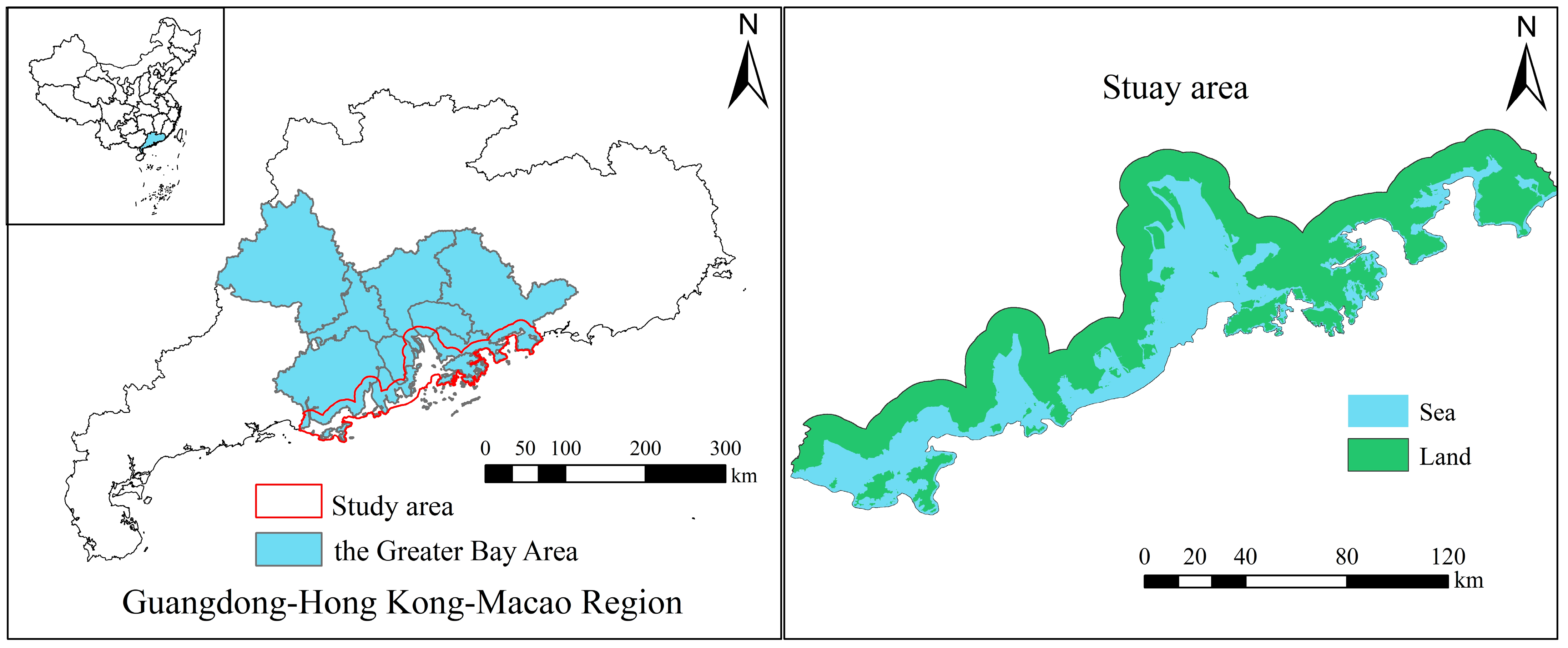
Figure 1. Overview of the Study Area.
Water 17 03566 g001
Figure 2. Land Cover Changes.
Water 17 03566 g002
Figure 3. Sankey Diagram of Land Use Transfer.
Water 17 03566 g003
Figure 4. Spatial distribution of ecosystem service values.
Water 17 03566 g004
Figure 5. Statistical chart of ecosystem service value quantities.
Water 17 03566 g005
Figure 6. Results of trade-off and synergy analysis.
Water 17 03566 g006
Figure 7. Spatial clustering analysis of each ecosystem service.
Water 17 03566 g007
Figure 8. Proportion of influence for each driving factor.
Water 17 03566 g008
Figure 9. RDA ordination results. Blue arrows represent ecosystem services; red dots represent driving factors.
Water 17 03566 g009
Table 1. Key Data and Sources.
Data TypeSource/ProcessingSpatial Resolution
Land CoverZenodo
https://zenodo.org/, accessed on 16 May 2025
30 m
Soil-Water DynamicsORNL DAAC
https://daac.ornl.gov/, accessed on 16 May 2025
250 m
PrecipitationNational Tibetan Plateau Scientific Data Center
https://data.tpdc.ac.cn/, accessed on 3 June 2025
1 km
EvapotranspirationNational Tibetan Plateau Scientific Data Center
https://data.tpdc.ac.cn/, accessed on 3 June 2025
1 km
Plant Available Water ContentNational Tibetan Plateau Scientific Data Center
https://data.tpdc.ac.cn/, accessed on 3 June 2025
1 km
6 m IsobathChina Oceanic Information Network
https://www.nmdis.org.cn/, accessed on 5 June 2025
30 m
DEMGEBCO
https://www.gebco.net/, accessed on 5 June 2025
500 m
Mangrove DistributionScienceDB
https://www.scidb.cn/, accessed on 5 June 2025
30 m
Aquaculture ZonesGlobal Change Scientific Research Data Publishing System
https://www.geodoi.ac.cn/, accessed on 5 June 2025
30 m
Coastal WetlandsGlobal Change Scientific Research Data Publishing System
https://www.geodoi.ac.cn/, accessed on 5 June 2025
30 m
NDVIResource and Environment Science Data Center
https://www.resdc.cn/, accessed on 13 June 2025
1 km
Population DensityZenodo
https://zenodo.org/, accessed on 16 May 2025
1 km
GDPResource and Environment Science Data Center
https://www.resdc.cn/, accessed on 13 June 2025
1 km
Nighttime LightsCenter for Sustainable Development Big Data International Research Center
https://sdg.casearth.cn/, accessed on 13 June 2025
1 km
Table 2. Overview of Ecosystem Service Types.
TypeService TypeModel AlgorithmVariable DescriptionReference
WYRegulating Service Y x = 1 A E T x P x P x Y x = Annual water yield of grid x (mm);
P x = Annual precipitation of grid x (mm);
A E T x = Actual evapotranspiration of grid x (mm)
[26,27,28,29]
URRegulating Service V R E i = 0.001 P i R E i p i x e l . a r e a
V R U , i = 0.001 P i R U i p i x e l . a r e a
V R E i = Retained stormwater volume per grid;
V R U , i = Runoff volume per grid;
P i = Annual precipitation (mm/yr);
p i x e l . a r e a = Area of each grid (m2);
R E i = Rainfall retention coefficient;
R U i = Runoff coefficient
[30]
UFRegulating Service R i = 1 Q p , i P R i = Runoff retention rate per grid;
Q p , i = Runoff per grid (mm);
P = Designed rainfall depth
[31]
SCRegulating Service A E R i = R K L S i U S L E i A E R i = Avoided erosion per grid;
U S L E i = Annual soil erosion per grid;
R K L S i U S L E i = Benefit of vegetation and good management practices
[32]
BCRegulating Service S t , t o t a l =
S t , p o o l + S t , b i o m a s s + S t , l i t t e r
S t , t o t a l = Total carbon storage at time t;
S t , p o o l = Sediment carbon storage;
S t , b i o m a s s = Biomass carbon storage;
S t , l i t t e r = Litter carbon storage
[33,34]
HQSupporting Service Q x j = H j 1 ( D x j z D x j z + k z ) j = Land use type;
Q x j = Habitat quality of grid x in type j;
H j = Habitat suitability of type j;
D x j = Habitat degradation of grid x in type j;
z = Normalization constant (2.5);
k = Half-saturation constant (0.5)
[35]
Table 3. Selected Driving Factors.
TypesFactorsAbbreviation
Natural factorsAnnual PrecipitationPRE
EvaporationEV
Digital Elevation ModelDEM
SlopeSP
Normalized Difference Vegetation IndexNDVI
Land-use factorsCultivated Land PercentageCL
Forest Land PercentageFL
Impervious Land PercentageIMP
Socio-economic factorsPopulation DensityPOP
Gross Domestic ProductGDP
Nighttime Light IndexNLD
Table 4. Results of spatial autocorrelation analysis (p < 0.001).
YearESMoran’s I
1990AWY0.860
SC0.827
USR0.863
UF0.878
CBC0.817
HQ0.784
2000AWY0.832
SC0.804
USR0.834
UF0.851
CBC0.852
HQ0.766
2010AWY0.832
SC0.804
USR0.836
UF0.847
CBC0.839
HQ0.784
2020AWY0.834
SC0.800
USR0.838
UF0.855
CBC0.831
HQ0.794
Disclaimer/Publisher’s Note: The statements, opinions and data contained in all publications are solely those of the individual author(s) and contributor(s) and not of MDPI and/or the editor(s). MDPI and/or the editor(s) disclaim responsibility for any injury to people or property resulting from any ideas, methods, instructions or products referred to in the content.