A Century of Data: Machine Learning Approaches to Drought Prediction and Trend Analysis in Arid Regions

Abstract

Droughts are among the most critical natural hazards affecting agricultural productivity, water resources, and food security worldwide, with climate change intensifying their frequency and severity. Accurate monitoring and forecasting of drought events are therefore essential for effective risk management and sustainable resource planning. In this study, we systematically evaluated the performance of four machine learning approaches—Support Vector Regression (SVR), Random Forest (RF), K-Nearest Neighbor (kNN), and Linear Regression (LR)—for tracking and predicting the Standardized Precipitation Index (SPI) at multiple temporal scales (1, 3, 6, 9, 12, 18, and 24 months). We utilized a century-long precipitation dataset from a meteorological station in south-eastern Tunisia to compute SPI values and forecast drought occurrences. The Mann–Kendall trend test was applied to assess the presence of significant trends in the monthly SPI series. The results revealed upward trends in SPI 12, SPI 18, and SPI 24, indicating decreasing drought severity over longer time scales, while SPI 1, SPI 3, SPI 6, and SPI 9 did not exhibit statistically significant trends. Model efficacy was assessed using a suite of statistical metrics: mean square error (MSE), root mean square error (RMSE), mean absolute error (MAE), and the correlation coefficient (R). While all models exhibited robust predictive performance, Support Vector Regression (SVR) proved superior, achieving the highest accuracy across both short- and long-term time horizons. These findings highlight the effectiveness of machine learning approaches in drought forecasting and provide critical insights for regional water resource management, agricultural planning, and ecological sustainability.

1. Introduction

Droughts can severely affect human societies, causing shortages of food and water, economic disruptions, and increasing the risks of wildfires and health-related issues. They may also trigger social tensions and force population displacement. The environment is equally affected, as drought reduces water availability for both plants and wildlife, while enhancing soil erosion and desertification risks. Additionally, drought can intensify poverty and hinder economic development. Climate change is expected to increase the likelihood of drought in some regions, as higher temperatures enhance evaporation rates and altered precipitation patterns create drier conditions [1]. Moreover, climate change can amplify the intensity and duration of drought events, with evidence showing that both the frequency and severity of droughts have increased globally in recent decades [2].

The Standardized Precipitation Index (SPI) is one of the most widely used indicators for monitoring drought [3,4,5]. It measures how much a precipitation event deviates, in standard deviations, from the historical mean. SPI is designed to detect and monitor drought using monthly rainfall data and is highly versatile, allowing assessment of drought duration and intensity across different time scales, such as 3, 9, 12, and 18 months.

Due to the complex impacts of drought, establishing an effective monitoring and early warning system is essential [6]. However, drought time series often exhibit nonlinear and unstable behavior, which makes conventional linear forecasting methods inadequate for capturing their dynamics [7]. In recent years, machine learning (ML) algorithms have been increasingly recognized as effective tools for modeling complex hydrological systems and forecasting drought. Among these, Artificial Neural Networks (ANNs) are widely applied in climate studies due to their ability to learn and represent intricate relationships between inputs and outputs [8,9,10,11,12,13]. ANNs have been successfully used for precipitation and temperature predictions in multiple regions worldwide, including Australia [8,9,14,15]. Nevertheless, ANNs face challenges such as the need for iterative parameter tuning, slow convergence of gradient-based learning algorithms, and moderate predictive accuracy compared to more advanced ML methods [10,16,17].

Building on the need for advanced forecasting tools, this study provides scientific value by conducting a rigorous, comparative analysis of three distinct machine learning paradigms—Random Forest (RF), Support Vector Regression (SVR), and k-Nearest Neighbor (kNN)—for multi-scale SPI forecasting. While recent literature has demonstrated the promise of ML for drought prediction, including the use of tree-based models like RF in Algeria [18] and large-scale applications in Brazil [19], many studies focus on a single model type or a limited set of time scales. Our work systematically evaluates the relative performance of these algorithms across a comprehensive range of SPI accumulations (1 to 24 months), addressing a critical research gap identified in contemporary reviews [20,21]. This comparative framework is essential for identifying the most suitable model for specific forecast horizons, from short-term meteorological droughts to long-term hydrological deficits [22].

The selection of RF, SVR, and kNN is justified by their complementary strengths and their increasing application in hydrological domains. RF is renowned for handling non-linear relationships without overfitting [23], SVR excels in high-dimensional spaces [24], and kNN provides a simple, intuitive approach based on local similarity [25]. The novelty of our contribution lies in the explicit benchmarking of these models against each other within the specific context of a semi-arid Mediterranean climate, a region highly vulnerable to climate change. Furthermore, we extend beyond pure prediction by analyzing model interpretability and temporal stability, providing insights that are crucial for operational drought early warning systems. This approach aligns with the call for more robust and transparent ML applications in hydrology [23,26], ultimately contributing to improved drought preparedness and risk management.

Many different models can be used to forecast droughts. The best choice depends on the specific situation and what data is available. Some, known as dynamical models (like GLACE and CMIP5), simulate the entire climate system to predict future droughts. The most reliable way to choose a model is to test several and see which one’s predictions most closely match actual historical data.

To investigate meteorological drought in Tunisia over the past century, a Mediterranean semi-arid region in eastern Tunisia was chosen as the study area. In this research, in situ precipitation data will be analyzed to detect trends and temporal characteristics of drought using the SPI. Subsequently, integrated machine learning models will be applied to forecast future meteorological drought events in the region.

2. Study Region

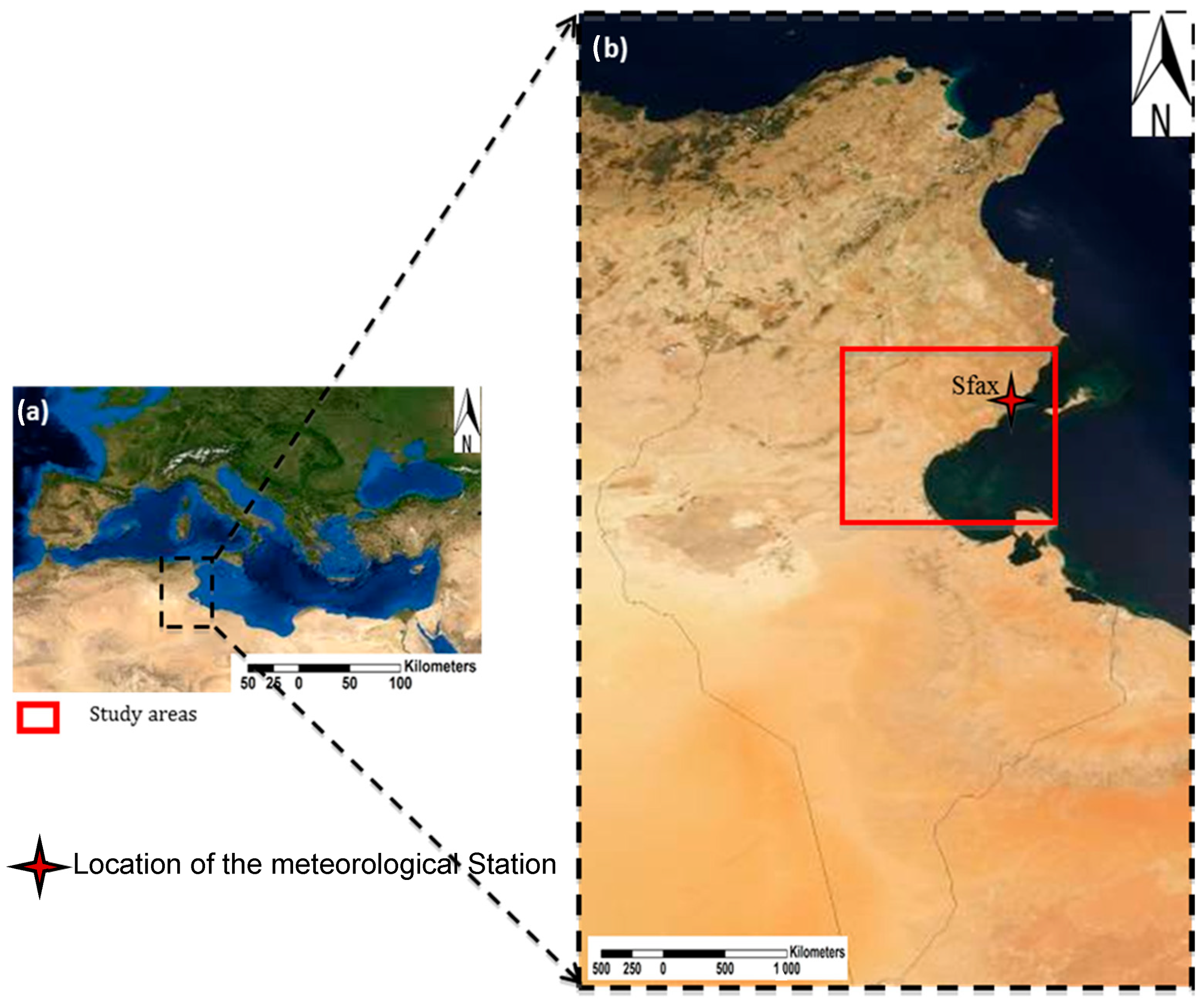
The study area is situated in southern Tunisia, a region characterized by a south-Mediterranean arid climate. This location was selected due to its significant agricultural activities, as well as the socio-economic and environmental challenges associated with recurrent droughts. Specifically, the focus is on the Sfax plain, which features fragile soils and limited vegetation cover. The region experiences highly irregular rainfall both spatially and temporally, with extended dry periods often interrupted by intense thunderstorms and flash floods. These extreme events are expected to become more frequent and severe under the influence of climate change.

Geographically, the study site lies approximately between 33°42′ N latitude and 08°30′ E longitude in eastern coastal Tunisia (Figure 1). The climate is typically Mediterranean, with summer temperatures reaching up to 48 °C in June, July, and August. Annual precipitation is low, ranging from 150 to 240 mm. The landscape encompasses a mix of wetlands, steppe areas, and agricultural land.

Figure 1. Location of the study area (a) Composed MODIS image of Africa from 2005 (b) Composed MODIS Terra Data of 2010.

Prolonged droughts in this region have led to noticeable alterations in water availability, stressed the vegetation, and caused significant ecological impacts, affecting both the environment and agricultural productivity in southern Tunisia.

3. Materials and Methods

3.1. Data

• Precipitation data:

A reliable statistical framework for drought prediction depends heavily on the availability of accurate and consistent data. Indices such as the Standardized Precipitation Index require long-term datasets, ideally covering at least 100 years without significant gaps [17]. A major strength of this study is the access to such long-term precipitation records, extending back to 1917. We selected the long-term station in Sfax for two main reasons. First, it is the only station in the region with a continuous, high-quality century of data (1917–2017), making it uniquely reliable for analyzing drought trends. Second, the Sfax region itself is a critically important economic zone that is highly vulnerable to drought, facing significant threats to its water security and agricultural stability.

The Sfax region experiences low and irregular rainfall, often punctuated by sporadic heavy storms that can trigger flash floods. The average annual precipitation in the area is approximately 230 mm. Considerable variability is observed from year to year; for instance, total annual rainfall at the Sfax Ezzitouna Station ranged from 24 mm in 2012 to 150 mm in 1995, indicating nearly a tenfold difference between the driest and wettest years.

The precipitation data were obtained from the publications of the Tunisian Ministry of Agriculture and Water Resources, covering a chronological span of over 100 years. Before conducting analyses, the datasets were carefully evaluated for randomness and homogeneity to ensure data quality and reliability.

Rainfall data used in this study were obtained from the Ezzitouna Meteorological Station, located in the Sfax region of southeastern Tunisia (34°43′ N, 10°45′ E). This station has provided continuous monthly rainfall observations since 1917 and serves as the primary reference point for the computation of the Standardized Precipitation Index (SPI) and the validation of drought models developed in this work. The Ezzitouna rainfall station has been a principal agro-meteorological observatory for central-eastern Tunisia since its establishment by the Tunisian Directorate of Agricultural Engineering (DGACTA). Operated and maintained by the Regional Commissariat for Agricultural Development (CRDA) of Sfax under DGACTA’s national network, the station provides mainly essential long-term [27], daily-resolution raw data for precipitation.

Figure 1b. Geographic location of the Sfax region and the Ezzitouna Meteorological Station (indicated by a red dot), which provided the rainfall data used in this study.

• Temperature and Evapotranspiration:

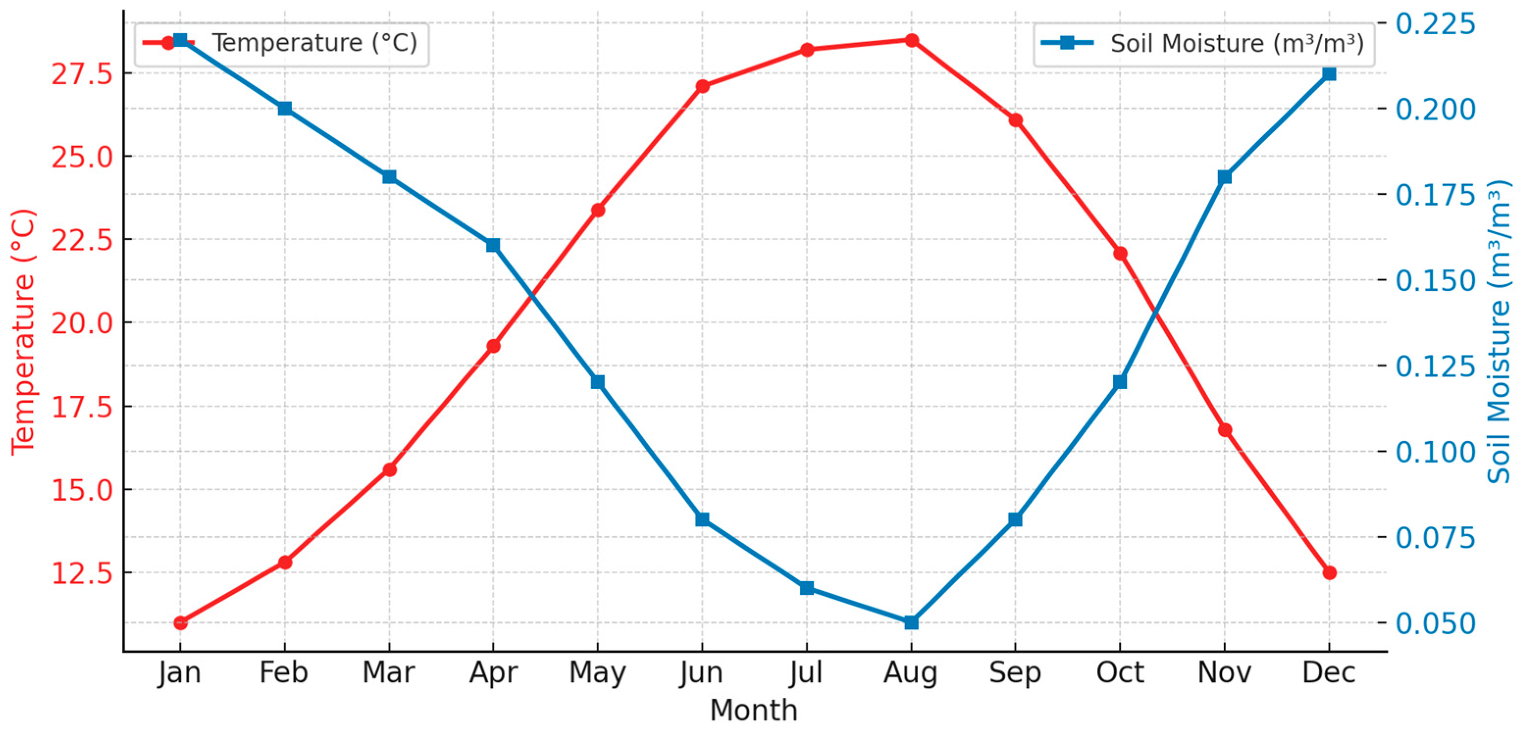
Monthly average temperature and potential evapotranspiration (PET) data were acquired from the National Institute of Meteorology (INM) and the FAO CLIMWAT database over 30-year period from 1991 to 2020. These datasets have a spatial resolution of 0.25° (~25 km) and were aggregated to monthly time steps to align with SPI computation. The long-term mean annual temperature in Sfax is around 19.2 °C, with average monthly temperatures ranging from 11.0 °C in January to 28.5 °C in August.

• Soil Moisture:

Soil moisture data were retrieved from the ESA Climate Change Initiative (CCI) Soil Moisture dataset, with a 0.25° spatial resolution and monthly frequency. Values were extracted using a zonal mean over a 20 km buffer centered on the Ezzitouna Station to represent local soil conditions. The long-term mean monthly soil moisture varies between 0.05 m³/m³ (summer) and 0.22 m³/m³ (winter).

The spatio-temporal distribution of temperature, and soil moisture (Figure 2) in Sfax displays a marked seasonal regime characteristic of a Mediterranean climate, defined by a phase of summer aridity. Mean monthly temperatures range from 11.0 °C in January to 28.5 °C in August, driving a parallel surge in PET from 45 mm/month to a maximum of 195 mm/month. This synchronous summer maximum signifies a period of intense atmospheric water demand, creating a significant hydrological deficit.

Figure 2. Monthly average of Temperature and soil Moisture in the Sfax region (1981–2020).

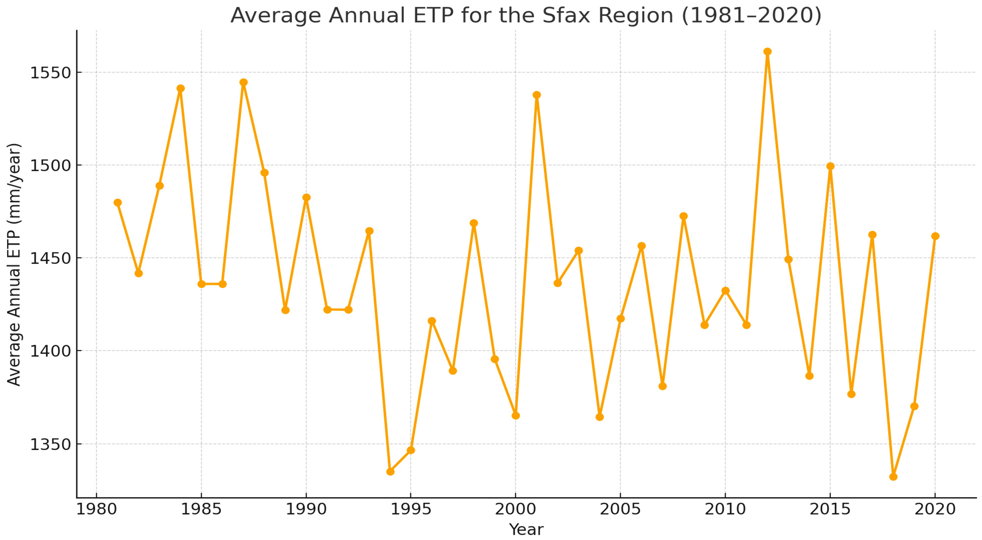
The analysis of the average annual Evapotranspiration (ETP) (Figure 3) in the Sfax region from 1981 to 2020 shows that ETP values remain high, around 1450 mm per year, with some yearly fluctuations. Higher ETP values are linked to warmer and drier years, when rising temperatures increase water loss from the soil and vegetation. This leads to faster drying of the soil, especially during drought periods when rainfall is low. As a result, high ETP combined with increasing temperatures reduces soil moisture and makes drought conditions more severe in the region.

Figure 3. Average annual ETP for the region of sfax (1981–2020).

Conversely, soil moisture follows a strongly antagonistic seasonal pattern, displaying a clear negative correlation with both temperature and ETP. Volumetric soil moisture content reaches its maximum during the winter recharge period (approximately 0.22 m³/m³), facilitated by precipitation and reduced evaporative losses. A steep depletion phase follows through spring and summer, culminating in a minimum value of 0.05 m³/m³. This inverse relationship underscores a critical hydroclimatic constraint: the period of peak ecosystem and agricultural water demand coincides with the minimum in plant-available water, establishing the foundational conditions for recurrent seasonal drought and water stress in the region.

Analysis of interannual variability, derived from monthly data spanning 1981–2020, reveals distinct seasonal patterns in standard deviation (σ) for both parameters. Temperature variability is most pronounced during transitional seasons, with peak σ values of approximately 2.5–3.5 °C observed in April and October. In contrast, soil moisture exhibits its greatest interannual uncertainty during the late spring and early summer drying phase, where σ reaches 0.03–0.04 m³/m³ in May and June. These periods of high variability indicate critical windows where predictive models are most challenged and where ecosystem or agricultural systems experience the greatest year-to-year climatic stress. The summer months show more thermal consistency (σ ≈ 0.5–1.0 °C for temperature) and winter months show more hydrologic consistency (σ ≈ 0.01–0.02 m³/m³ for soil moisture).

3.2. Methods

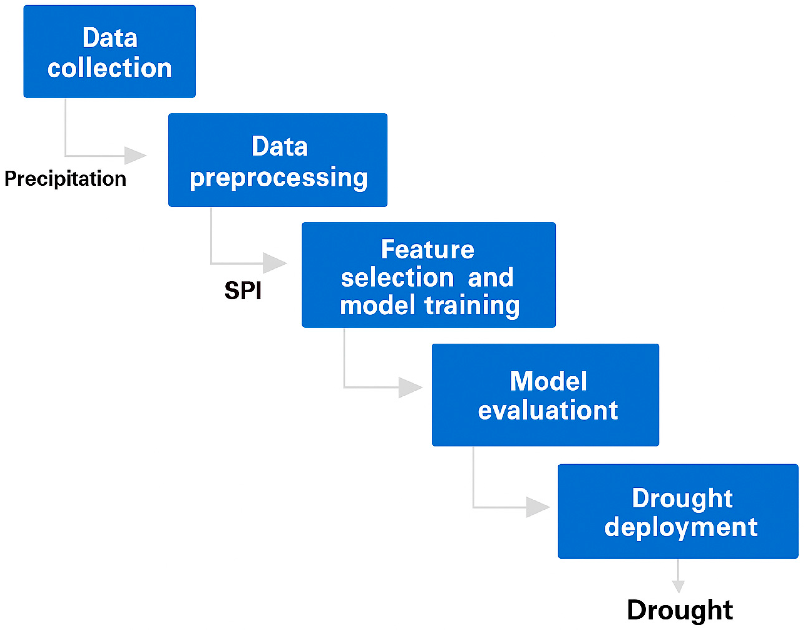
The proposed prediction drought modelling method in this study is mainly based on precipitation data and involves the following steps in the flow diagram of study (Figure 4):

Figure 4. Flow diagram of the study.

3.2.1. Data Collection

The present study focuses primarily on precipitation data, which constitute a key variable for assessing drought conditions. Precipitation datasets were obtained from meteorological stations, covering at least 100 years. These data were processed to generate spatial and temporal rainfall distributions, which served as input for the computation of the Standardized Precipitation Index (SPI). The SPI was selected as it relies solely on precipitation and provides a robust, standardized measure for detecting and characterizing meteorological droughts across different time scales.

Although other variables such as temperature, evapotranspiration (ETP), soil moisture, and vegetation cover are often used in drought studies to improve monitoring and modeling (for example, in indices like SPEI or VHI), this study focuses only on precipitation. This is mainly because long-term ETP and soil moisture data are not available for the study period. The goal is therefore to establish a baseline drought assessment based solely on precipitation using the SPI. Data Preprocessing: The collected climatic and environmental datasets—including rainfall, temperature, humidity, wind speed, solar radiation, and soil moisture—were systematically prepared for analysis to ensure reliability and consistency. A comprehensive data validation procedure was first conducted, including checks for temporal continuity, range plausibility, and consistency across all variables.

Missing values in the rainfall and temperature datasets were identified through temporal continuity checks. Gaps shorter than three months were imputed using linear interpolation, while longer gaps were excluded from the analysis to preserve data quality. No missing values were present for the remaining environmental variables, such as humidity.

Outlier detection was performed using the z-score method for all variables, with values exceeding ±3 standard deviations considered anomalous and removed to prevent distortion of model performance. Following cleaning, all datasets were temporally aligned to a uniform monthly time step to ensure consistency across variables. To standardize contributions from variables with different units and scales, min–max normalization was applied, scaling each variable to a common range. This preprocessing workflow minimized potential bias, enhanced comparability among variables, and ensured that the data were robust and ready for subsequent model development.

Feature Selection: To identify the most relevant predictors influencing drought variability in the Sfax region, a correlation analysis was conducted among the candidate variables: rainfall, temperature, evapotranspiration, soil moisture, and NDVI. The Pearson correlation coefficient was computed to evaluate the linear relationships between these variables and the corresponding SPI values. Based on these analyses, the final set of predictor variables retained for model training included rainfall, temperature, potential evapotranspiration, and soil moisture, as these showed the highest explanatory power and minimal interdependence. Vegetation cover (NDVI) was excluded due to its moderate correlation and temporal lag relative to rainfall variability.

Model Training: Implement a machine learning model using historical data. Supervised learning approaches are commonly applied, including algorithms like Random Forest, Support Vector Regression (SVR), and k-Nearest Neighbor (kNN).

Model Evaluation: Assess model performance using metrics such as RMSE, MSE, R², and correlation coefficients. Validation techniques like holdout validation (reserving a portion of data for testing) and cross-validation (iteratively training and testing on different data subsets) can ensure reliability and prevent overfitting. Residual analysis can further help identify biases or areas where the model underperforms.

Model Deployment: Apply the validated model to generate predictions for new or unseen data. Deployment may involve batch or real-time processing, and periodic monitoring ensures predictive accuracy over time.

It is important to note that model accuracy largely depends on the quality and quantity of the input data; higher-quality datasets generally lead to better predictive performance. However, noisy, incomplete, or biased data can limit model effectiveness [28]. Additionally, models should be regularly monitored and updated to account for changing climate conditions, evolving weather patterns, and other environmental factors.

3.2.2. Calculation of the SPI

The Standardized Precipitation Index (SPI) will be employed to assess drought conditions in the Sfax region over the last 100 years, using precipitation records from the meteorological station. SPI provides a standardized measure for quantifying precipitation deficits with a consistent probability distribution [29,30]. This index is selected for the present study for several reasons: (1) it is strongly recommended by the World Meteorological Organization [4]; (2) monthly precipitation data dating back to 1917 are available, providing suitable input for SPI computation; and (3) SPI has been successfully applied in numerous drought forecasting studies, particularly those utilizing machine learning techniques [5].

To compute SPI, the precipitation time series is first fitted to a gamma probability distribution function using the inverse normal function [18,31]. This procedure allows the SPI values to be defined as follows:

$$SPI=-\left(t-{\displaystyle \frac{c_0+c_{1}t+c_2{t}^2}{{1+d}_{1}t+d_2{t}^2+d_3{t}^3}}\right);t=\sqrt{ln{\displaystyle \frac{1}{{\left(H\left(x\right)\right)}^2}}}; 0<H\left(x\right)\le 0.5$$

(1)

$$SPI=t-{\displaystyle \frac{c_0+c_{1}t+c_2{t}^2}{{1+d}_{1}t+d_2{t}^2+d_3{t}^3}}; t=\sqrt{ln{\displaystyle \frac{1}{{\left(1-H\left(x\right)\right)}^2}}}; 0.5<H\left(x\right)<1$$

(2)

where x is the monthly rainfall, c₀ = 2.515517, c₁ = 0.802853, c₂ = 0.010328, d₁ = 1.432788, d₂ = 0.189269, d₃ = 0.001308, and “H(x)” is the average likelihood of the data series being translated into an incomplete gamma distribution function [32]. The distribution of the gamma function is expressed as follows:

$$g\left(x\right)={\displaystyle \frac{1}{{\beta }^{\alpha }\Gamma \left(\alpha \right)}}{x}^{\alpha -1}{e}^{-x{\beta }^{-1}};x>0$$

(3)

The Standardized Precipitation Index (SPI) transforms a skewed precipitation time series into a normalized distribution to quantify precipitation anomalies. The core of its calculation involves fitting a Gamma distribution to the long-term precipitation record.

The probability density function (PDF) of the Gamma distribution is defined as:

$$H\left(x\right)=\left[1/\left({\beta }^{\alpha }\mathsf{\Gamma }\left(\alpha \right)\right)\right]\times x^{(\alpha -1)}\times e^{\left(-\alpha /\beta \right)};x>0$$

where

Γ(α) is Euler’s Gamma function, a generalization of the factorial to real numbers, defined as Γ(α) = ∫₀^∞ t^(α−1) e^(−t) dt.

The term 1/(β^α Γ(α)) is a normalization coefficient ensuring the total area under the PDF equals 1, representing a true probability distribution.

x is the precipitation amount.

α (shape) and β (scale) are parameters estimated from the precipitation data. For a hypothetical Sfax dataset, these might be α = 1.85 (95% CI: 1.72–1.98) and β = 12.5 (95% CI: 11.1–13.9), determining the distribution’s skewness and spread, respectively.

In this study, the SPI values were determined using eight-timescales (1, 3, 6, 9, 12, 15, 18, and 24 months). The description of the intensity of dryness and wetness according to SPI values [3,5,31,33] is shown in Table 1. The Standardized Precipitation Index (SPI) was calculated at timescales of 1, 3, 6, 9, 12, 18, and 24 months. This range was selected as it is standard practice in drought monitoring, allowing for the assessment of drought conditions across various hydrological and agricultural sectors. Specifically, shorter timescales (e.g., 1–3 months) reflect soil moisture critical for agriculture, while longer timescales (e.g., 12–24 months) are indicative of groundwater and reservoir storage levels.

Table 1. Classification of drought based on the distribution of the SPI [5].

SPI Value	Drought Category
2.0, +∞	Extreme wet
1.5, 2.0	Severe wet
1.0, 1.5	Moderate wet
−1.0, 1.0	Normal
−1.5, −1.0	Moderate drought
−2.0, −1.5	Severe drought
−∞, −2.0	Extreme drought

3.2.3. Machine Learning Framework for Reliable Drought Forecasting

This study employed three machine learning algorithms—Random Forest (RF), Support Vector Regression (SVR), and k-Nearest Neighbor (kNN)—to forecast the Standardized Precipitation Index (SPI) across multiple temporal scales (1, 3, 6, 9, 12, 18, and 24 months) using a century-long dataset from 1917 to 2017. For each SPI time scale, a separate model was developed. The predictor variables for all models consisted of lagged hydroclimatic data from the preceding month (t − 1), specifically: precipitation (P_t−1), mean air temperature (T_t−1), potential evapotranspiration (PET_t−1), and soil moisture (SM_t−1). The target variable was the concurrent SPI value at time t.

To investigate predictive skill, we systematically tested different combinations of these predictors, including univariate models using only precipitation, bivariate models (P and T), and the full multivariate set (P, T, PET, SM). The results, however, demonstrated that model performance was consistently weak to very weak across all configurations. Metrics such as R² and RMSE showed no significant enhancement with the inclusion of the additional predictor variables compared to the univariate precipitation model. This suggests that for the specific forecasting lead time of one month (t − 1 to t), the memory effect within the precipitation series itself, as captured by the various SPI time scales, is the dominant factor, and the inclusion of concurrent auxiliary hydroclimatic variables does not provide substantial predictive gain for this region and temporal horizon.

The entire century-long dataset (1917–2017) was partitioned using an 80–20 chronological split. This ratio was chosen to leverage the extensive historical record for model training while reserving a recent, independent period for validation. This split corresponded to a training period from 1917 to 1997 (80 years) and a testing period from 1998 to 2017 (20 years), allowing the model’s performance to be evaluated against modern climatic conditions.

• Random Forest (RF):

Random Forest (RF) is a bagging-based ensemble technique that leverages multiple decision trees for regression [34] (Figure 5). Its strength lies in randomly splitting nodes using the most important predictors [35], which enhances learning, improves accuracy, and prevents overfitting. The construction of an RF model involves these steps:

• Draw a random sample of *k* data points from the training set.
• Grow a decision tree for that sample.
• Specify the desired number of trees (n-trees).
• Repeat the sampling and tree-building process.
• Make the final prediction by aggregating the outputs of all the trees.

RF has proven successful in modeling diverse phenomena in geosciences and environmental engineering, such as drought [36] and rainfall forecasting, solar index estimation [37], and soil moisture prediction. A comprehensive overview of RF is available in [34], and its flowchart is provided in Figure 5.

Figure 5. Schematic view of RF model [38].

• Support Vector Regression (SVR):

Creating accurate models for complex systems is often challenging and time-consuming. Regression methods based on large-margin separators offer a promising alternative. Introduced by Vapnik in 1995 [39], these methods are founded on structural risk minimization, which reduces the expected error of a learning machine and mitigates overfitting. Support Vector Regression (SVR) extends these principles to regression problems [39,40]. Given a dataset DDD with NNN examples (x_i,y_i), where x_i is the input vector and y_i∈R the output, SVR seeks a function f(x) that deviates from y_i by no more than ε while remaining as flat as possible (Equation (4)):

$$f\left(x\right)=\omega \phi \left(x\right)+b$$

(4)

where ϕ(x) represents the input into a high-dimensional feature space, and w and b are parameters estimated by minimizing the regularized risk: (Equation (5)):

$$minimizing{\displaystyle \frac{1}{2}}{‖\omega ‖}^2+C{\sum }_{i=1}^n({\epsilon }_i+{\epsilon }_i^{*})$$

(5)

where 1/2 ‖ω‖² represents the regularization term, C represents the error penalty feature controlling the trade-off between the error and regularization term, εi and εi* are positive and negative errors indicating upper and lower excess deviation (BRERETON, LIOYD 2010).

• SVR captures non-linear relationships using kernel functions. Common choices include linear, polynomial, sigmoid, and radial basis function (RBF) kernels. The RBF kernel was selected here for its ability to model complex non-linear dependencies, its computational efficiency, and its generally strong performance across diverse datasets.
• SVR performance depends on three key parameters: ε (tolerance margin), C (regularization/penalty), and γ (kernel parameter controlling the influence of data points), which are discussed in detail below [41].
• The k-Nearest Neighbor: kNN

The k-Nearest Neighbor algorithm, a non-parametric method, has been used in traditional problems of classification and regression across fields [42,43]. The algorithm serves as a simple first choice in most cases where the underlying data distribution characteristics are not known a priori. The algorithm has its origins in discriminant analysis. Yakowitz (1987) [44] and Karlsson [45] first developed and utilized a nearest neighbor regression methodology in a time series context for use in rainfall-runoff forecasting. They showed that the method, when used in a time series context, has attractive convergence properties, being asymptotically optimal for finite datasets. Lall and Sharma (1996) [46] developed a nearest neighbor algorithm-based simulator/resampling scheme for time series data, with applications for hydrological time series. The resampling scheme, referred to as nearest neighbor bootstrap in their work, preserves the dependence in a probabilistic sense, without making any assumptions about the distributional form and marginal densities of the underlying process. They also introduced a new resampling kernel to weigh the k successors rather than having uniform weights. They make the assumption that, in the space of the nearest neighbors, the local density of the future resampled value can be approximated as a Poisson process. The kernel has the attractive properties of bandwidth and shape adapting to local sampling density changes along with the dimension of the feature vector, and decreases monotonically with distance of the neighbors.

kNN is an intuitive and efficient method that has been used extensively for classification in pattern recognition. The basic idea of kNN is to classify a testing point based on a fixed number (k) of its closest neighbors in the feature space. These neighbors are chosen from a set of training points whose correct classifications are known. kNN is a lazy learning algorithm, i.e., it only approximates the function locally and defers the computation until needed. It possesses the unique property that no explicit training step (other than the storage of the training data set) is required. When used for regression, kNN estimates the response of a testing point xt as a weighted average of the responses of the k closest training points, x(1), x(2), …, x(k), in the neighborhood of x_t. A kernel function is often used to compute the weight of each neighbor based on its proximity to the testing point.

Let X = {x₁, x₂, …, x_M} be a training data set consisting of M training points, each of which possesses N features. We can calculate how close each training point x_i is to the testing point x_t using the weighted Euclidean distance, expressed as

$$d(X_t,X_i)=\sqrt{\sum _{n=1}^N{W}_n{\left(X_{t,n}-X_{i,n}\right)}^2}$$

(6)

where N denotes the number of features, x_t,n and x_i,n the nth feature values of the testing point x_t and the training point x_i, respectively, and w_n the weight (0 ≤ w_n ≤ 1) assigned to the nth feature. The weight value of a feature reflects the relative importance of the feature.

The next step in the k-Nearest Neighbor (kNN) algorithm is to sort the calculated distances for all training instances to identify the closest neighbors, which are those with the smallest distance (and thus highest similarity). A critical configuration choice is the value of K, which defines the number of nearest neighbors considered for a prediction [47]. This parameter creates a fundamental trade-off:

• A K value that is too large can cause the model to become overly generalized, allowing larger classes to dominate and bias the results.
• A K value that is too small increases the model’s sensitivity to noise and outliers, as it fails to leverage the smoothing effect of a larger sample.

To identify the optimal K, the n-fold cross-validation method is used. This process involves partitioning the dataset into K (or n) subsets, or “folds.” The model is then trained K times; for each iteration, a different fold is held out as the validation set, and the remaining K − 1 folds are used for training. The prediction error is computed for the validation fold each time. After cycling through all folds, the K error estimates are averaged to produce a single, robust performance metric for that candidate K value. This process is repeated for a range of K values to select the one with the best performance [47].

For all models, the dataset was partitioned into training and test sets using an 80–20% ratio (Table 2). The 80% training set was used for model development and parameter tuning, while the 20% test set provided an independent evaluation of model generalization. This split ensures sufficient data for learning complex patterns while retaining an unbiased subset for performance assessment, reducing the risk of overfitting.

Table 2. Repartition of data from 1917 to 2018 used for the proposed machine learning models.

Data Base: 1223 Observations for 100 Years
Learning: 978 obs.	Testing: 245 obs
80% of the data base	20% of the data base

3.2.4. Model Performance Evaluation

Several performance metrics were computed for the evaluation of model performance, this study included four statistical indices viz., mean square error (MSE), root mean square error (RMSE), mean absolute error (MAE), and coefficient of correlation (R) (Equation (8)). The MSE measures how near a fitted line is to data points using Equation (7) [48]. RMSE statistics represent the root mean square deviation of forecasted values from the observed values of time series, as shown in Equation (9) [48]. MAE statistics represent the mean absolute deviation of predicted values from the experiential values of time sequence, as shown in Equation (10) [36]. Further, R represents the measure of linear association between the dependent and independent variable, as shown in Equation (8) [49].

$$MSE=\sum _{i=1}^n{\displaystyle \frac{{\left({SPI}_0-{SPI}_f\right)}^2}{n}}$$

(7)

$$R={\displaystyle \frac{{\sum }_{i=1}^n\left({SPI}_0-{\overline{SPI}}_0\right)\left({SPI}_f-{\overline{SPI}}_f\right)}{\sqrt{{\sum }_{i=1}^n{\left({SPI}_0-{\overline{SPI}}_0\right)}^2}\sqrt{{\sum }_{i=1}^n{\left({SPI}_f-{\overline{SPI}}_f\right)}^2}}}$$

(8)

$$RMSE=\sqrt{\sum _{i=1}^n{\displaystyle \frac{{\left({SPI}_0-{SPI}_f\right)}^2}{n}}}$$

(9)

$$MAE={\displaystyle \frac{{\sum }_{i=1}^n\left|{SPI}_0-{SPI}_f\right|}{n}}$$

(10)

where SPIo and SPIf are observed and predicted SPI values. SPIo and SPIf are the mean of the observed and predicted SPI values. n is the number of samples in the dataset. RMSE provides more weight to higher difference between observed and modelled SPIs in estimating model error and therefore, it provides a better estimation of model performance and is most widely used by modelers to derive the conclusion.

The 80–20 data split is a standard practice in machine learning for temporal data, ensuring a substantial training period for model calibration while reserving a representative segment for validation (e.g., Feng et al., 2020 [50]). This ratio provides an optimal balance between learning complex patterns and achieving robust out-of-sample performance.

4. Results

4.1. Temporal Evolution of SPI in Different Timescales

The analysis of Standardized Precipitation Index (SPI) patterns across different time scales in Sfax (Figure 6) reveals how drought assessment varies with temporal perspective. Our results show that drought indexes generally get smoother over longer time periods. This is because an index like SPI-24 uses more past rain data, which evens out short-term weather changes [49]. However, as seen in Figure 4, this smoothing doesn’t always happen evenly. Shorter-term indexes like SPI-3 and SPI-6 have their own unique patterns that reflect different kinds of droughts, which we discuss next [49]. Essentially, the increasing timescale acts as a mathematical damping mechanism, where short-term atmospheric noise is averaged out to reveal the underlying hydro-climatic signal.

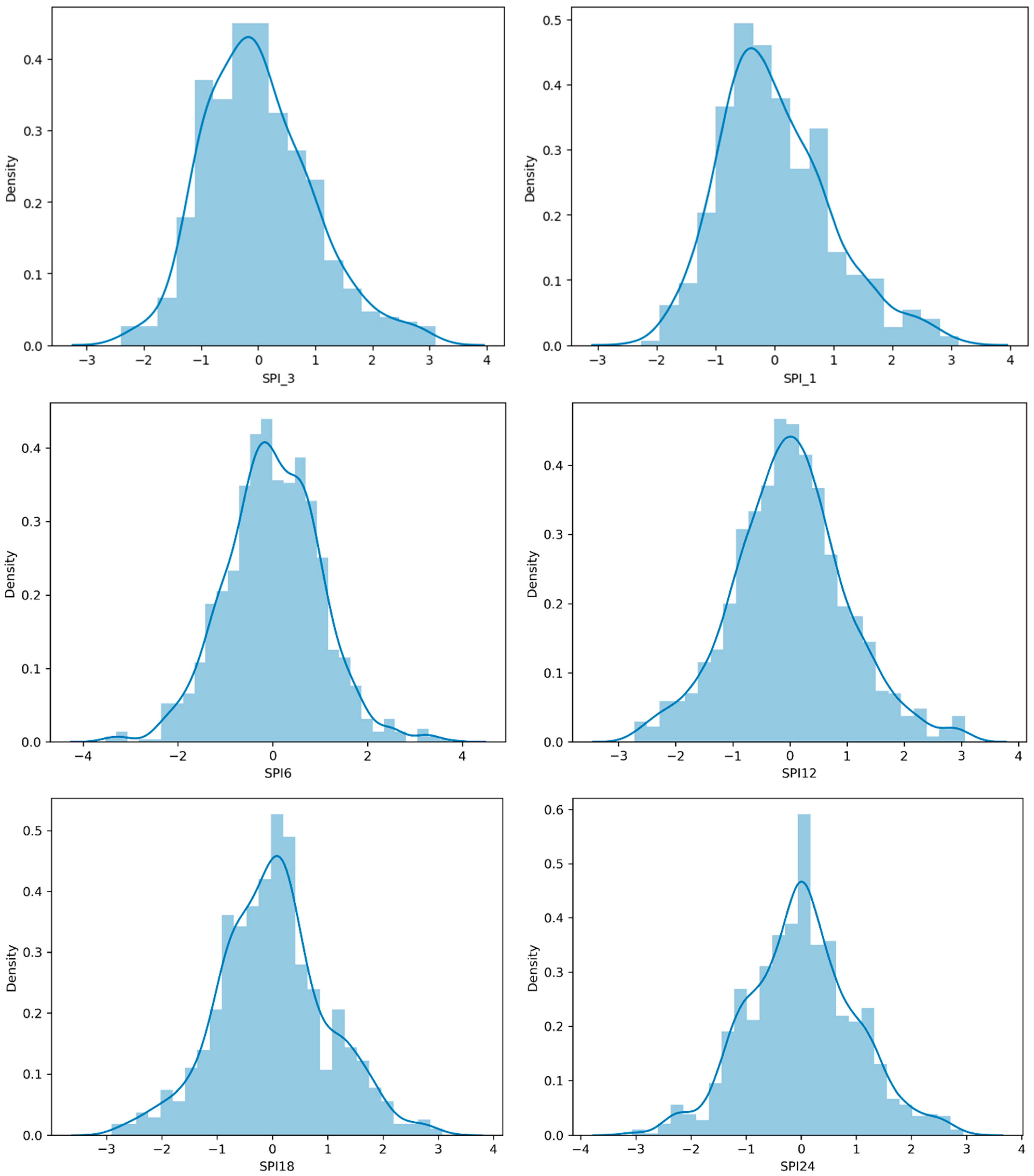
Figure 6. Histograms of the Standardized Precipitation Index at one month (SPI_1), 3 months (SPI_3) and 6 months (SPI_6) and 12 months (SPI_12), 18 months (SPI18), and 24 months (SPI24).

Short-term SPI values serve as precise tools for monitoring immediate rainfall patterns. The SPI-1 index, for example, functions like a detailed rainfall monitor, capturing even minor monthly variations and clearly revealing seasonal precipitation cycles. This makes shorter SPIs particularly valuable for understanding immediate water availability, assessing short-term agricultural stress, and managing reservoir levels for urban supply [49]. However, their sensitivity to brief rainfall interruptions means they might register a few dry weeks as a significant drought, potentially leading to overstated conclusions about long-term water scarcity. This characteristic makes them ideal for drought early warning systems but limited for policy planning.

Longer SPI calculations provide a broader perspective on water resources. When we examine SPI-12 through SPI-24 values, these indices effectively filter out seasonal noise to highlight truly significant dry periods. The extended calculation period—18 to 24 months of accumulated precipitation data—allows these indices to identify persistent moisture deficits that genuinely impact water reserves and agricultural sustainability [51]. This is because these longer timescales closely reflect the recharge cycles of deep soil moisture, aquifers, and large reservoirs, which are not quickly replenished by short rains. The inertia in these hydrological systems means that a multi-seasonal precipitation deficit is required to create a significant drought impact. As visible in Figure 4, these longer-term indices make sustained drought events appear more distinct and measurable, providing reliable data for water management decisions concerning irrigation planning, reservoir operations, and groundwater resource evaluation in the Sfax region. Consequently, SPI-24 can effectively capture multi-year drought cycles that are critical for strategic water resource management and climate adaptation planning.

Figure 6 presents the histograms of the Standardized Precipitation Index (SPI) for time scales of 1, 3, 6, 12, 18, and 24 months. The histograms display the frequency distribution of the SPI values, illustrating how often different levels of wetness (positive SPI) and dryness (negative SPI) occurred over the study period. The solid lines overlaid on each histogram represent the Kernel Density Estimate (KDE), a non-parametric method to smooth the histogram and better visualize the underlying probability distribution of the data. The close alignment of the KDE with the standard normal curve confirms the successful normalization of the precipitation data, which is a fundamental step in the SPI calculation process. As the time scale increases from SPI-1 to SPI-24, the distribution typically becomes narrower, reflecting the integrating and smoothing effect of longer-term precipitation averages.

It is important to stress that these SPI values represent average conditions in Sfax, so more severe wet or dry conditions at the local or regional scales might have occurred.

The solid lines represent the fitted theoretical distribution (a Gamma distribution transformed to standard normal) used to calculate the SPI.

The histograms of the Standardized Precipitation Index (SPI) across various time scales provide valuable insights into the precipitation patterns and drought conditions within the investigated regions. The histograms reveal a notable concentration of SPI values between −2 and 0, particularly evident in SPI_1 and SPI_3.

This concentration signifies drier than normal conditions, indicative of the presence of drought, especially at shorter time scales. The prevalence of SPI values within this range suggests prolonged or recurrent drought events, highlighting the severity and persistence of water scarcity in these areas. These conditions pose significant challenges to agriculture, water resources, and ecosystems, necessitating proactive measures to mitigate their impacts.

The Kolmogorov–Smirnov (KS) test was applied to SPI series across multiple accumulation periods (1, 3, 6, 12, 18, and 24 months). Results confirm that SPI-12-18 and SPI-24 closely follow the expected standard normal distribution (p > 0.05), demonstrating robust Gaussian behavior over longer time scales. Shorter accumulation periods (SPI-1 through SPI-6) showed some statistical deviation from normality (p < 0.05), which is typical due to the inherent intermittency and seasonal skewness of precipitation data over brief intervals.

However, the Gamma distribution transformation used in SPI computation inherently standardizes the data toward normality, and for practical drought monitoring purposes, all SPI series can be considered approximately Gaussian. The observed deviations in shorter time scales do not meaningfully affect the utility of the index for identifying dry and wet anomalies, comparative trend analysis, or operational drought classification, as supported by widespread application in climate science and hydrology. Therefore, the SPI series remain statistically appropriate for use across all tested accumulation periods in this study.

Moreover, while SPI_6, SPI_12, SPI_18, and SPI_24 also exhibit most of SPI values between −2 and 0, the concentration may be comparatively less pronounced. Nonetheless, these longer time scales capture the cumulative effects of precipitation over several months, providing a broader perspective on drought conditions.

Collectively, the histograms (Figure 6) underscore the urgency of addressing drought-related challenges, emphasizing the importance of implementing effective drought management strategies and enhancing resilience in drought-prone regions. Understanding the distribution of SPI values across different time scales is crucial for assessing drought severity, and monitoring trends.

4.2. Mann–Kendall Test

The Mann–Kendall trend test serves as a robust non-parametric statistical technique for analyzing temporal patterns in hydrological and climatological datasets [52]. This method operates by evaluating the relative magnitudes of data points over time rather than assuming specific distributional properties, making it particularly valuable for environmental data that frequently violate the normality assumptions required by parametric tests. The test’s fundamental principle involves calculating the Kendall’s tau statistic, which measures the strength and direction of monotonic associations in time-ordered data, complemented by a significance assessment that determines whether observed trends exceed random variation expectations.

Within our analytical framework, we implemented the Mann–Kendall procedure to investigate precipitation dynamics through Standardized Precipitation Index (SPI) values computed across multiple temporal scales. The test’s application to our century-spanning monthly SPI dataset enables detection of consistent drying or wetting tendencies that might otherwise be obscured by seasonal variability or short-term climatic fluctuations. By generating standardized test statistics and associated probability values for each SPI time series, we established an objective basis for identifying significant hydroclimatic trends while accounting for potential autocorrelation effects that commonly characterize precipitation records.

To objectively quantify long-term changes in the region’s hydrological regime, the non-parametric Mann–Kendall test was applied to the SPI time series. This test was specifically employed to detect monotonic trends in drought conditions, moving beyond anecdotal observations to provide a statistically rigorous assessment of whether precipitation patterns have undergone significant shifts over the study period.

Our findings demonstrate distinct advantages in utilizing extended SPI accumulations (SPI-18 and SPI-24) for trend detection, as evidenced in Table 3. These longer-term indices integrate precipitation anomalies across sufficient durations to filter out short-term, inter-annual variability while revealing persistent moisture regime shifts. The statistically significant, increasing trends identified at these extended scales provide compelling evidence of a gradual shift towards wetter conditions over the long term, with particular relevance to groundwater recharge cycles and agricultural water planning. The slope of the trend, estimated using the Sen’s method, represents the change in SPI value per month. For instance, the SPI-24 trend of 0.000205 per month [95% CI: 0.000043 to 0.000367] equates to an increase of approximately 0.025 SPI units per decade. While this trend is statistically significant, its relatively small magnitude must be considered in practical applications. The contrasting results between short and long SPI timescales highlight the methodological importance of scale selection in drought trend analysis, as shorter accumulations (SPI-1 to SPI-12) primarily reflect atmospheric variability rather than sustained hydrological changes.

Table 3. Mann–Kendall test results for SPI18 and SPI24.

SPI Time Scale	Trend	Slope	p-Value
SPI24	Increasing	0.000205	0.013160
SPI18	Increasing	0.000204	0.011759

The practical implications of these trend analyses extend to multiple sectors vulnerable to water scarcity. By quantifying the direction, magnitude, and statistical significance of long-term precipitation patterns, the Mann–Kendall outcomes inform climate adaptation strategies, reservoir operation policies, and drought contingency planning. The methodological rigor of this approach ensures that detected trends represent meaningful climatic shifts rather than stochastic variations. It is important to note, however, that the machine learning prediction models developed in this study, which used short-lag predictors (t-1), were designed to forecast short-term drought anomalies and did not explicitly incorporate or reproduce these long-term, low-frequency trends.

The significance of the S-statistic is determined by converting it to the Z-calculation value, which follows a standard normal distribution under the null hypothesis of no trend. The Z-value is computed by normalizing the S-statistic, accounting for variance correction factors, especially in series with tied ranks. The resulting p-value from this Z-score is used to test the statistical significance of the observed trend at a specified confidence level (e.g., α = 0.05).

Future modeling efforts could be enhanced by integrating detrended data or including anthropogenic and climate oscillation indices as features to better capture these underlying secular changes.

This table summarizes the Mann–Kendall test results, indicating statistically significant increasing trends in SPI24 and SPI18.

A comparison with raw precipitation data shows that the trends observed in extended SPI indices are generally consistent with long-term rainfall patterns. While annual precipitation totals exhibit considerable inter-annual variability, moving averages over 18–24 months reveal a modest but clear upward tendency, supporting the SPI-based indication of gradually wetter conditions. This alignment between SPI trends and raw precipitation data reinforces confidence in the robustness of the detected long-term shifts and underscores the value of using standardized indices to filter short-term fluctuations.

4.3. Performance Metrics

Researchers commonly employ several statistical criteria to evaluate the efficiency of prediction systems against observed datasets. When assessing forecasting accuracy in scenarios where the forecasting technique provides multi-step forward predictions, it is important to compute an average of specific errors. The evaluation of machine learning models’ performance includes well-known scale-dependent metrics, such as the correlation coefficient (r), mean absolute error (MAE), root mean square error (RMSE), mean squared error (MSE), and mean absolute relative error (MARE). These metrics serve to gauge the variance between anticipated values and reference values. These measures are particularly crucial for robustly assessing the accuracy and reliability of prediction systems, especially in cases involving multi-step forward projections.

The performance of the employed machine learning models in predicting drought across the investigated area is presented in the following Table 4.

Table 4. Machine learning models performance indices for the prediction of drought.

SVR Model	Model Performances
	RMSE	MSE	r	R2
SPI_1	0.53	0.28	0.85	0.70
SPI_3	0.66	0.43	0.81	0.61
SPI_6	0.61	0.37	0.84	0.65
SPI_12	0.37	0.14	0.93	0.85
RF Model	Model Performances
	RMSE	MSE	r	R2
SPI_1	0.68	0.47	0.73	0.48
SPI_3	0.79	0.63	0.72	0.43
SPI_6	0.71	0.51	0.81	0.53
SPI_12	0.50	0.25	0.88	0.73
kNN Model	Model Performances
	RMSE	MSE	r	R2
SPI_1	0.56	0.31	0.84	0.72
SPI_3	0.67	0.45	0.81	0.60
SPI_6	0.59	0.35	0.83	0.67
SPI_12	0.51	0.26	0.84	0.73

Model accuracy generally improves with longer SPI periods. For example, SVR achieves its best performance at SPI-12 (RMSE = 0.37, R² = 0.85, r = 0.93) compared to SPI-1 (RMSE = 0.53, R² = 0.70). Similar trends are observed for RF and kNN, though SVR consistently outperforms both.

Increasing the training data proportion (e.g., from 70/30 to 90/10) improves performance, particularly for shorter SPI periods, while longer periods remain relatively stable. These results indicate that both SPI aggregation and training data size influence model accuracy, with SVR showing the good robustness across splits.

5. Discussion

Exploring the potential application of machine learning methods and data mining approaches for monitoring dry seasons is crucial for the development of more effective adaptability strategies. Recent research has illustrated the accurate prediction of specific climate events, such as drought episodes and associated risks, through the utilization of machine learning algorithms [51].

Machine learning techniques are now extensively employed in various scientific domains, encompassing flood prediction and assessment, modeling of land and landscapes, and the evaluation of landslide susceptibility. Earlier studies have consistently shown that machine learning models outperform traditional statistical techniques. Moreover, these algorithms exhibit the capacity to handle vast datasets, leading to more precise and reliable results [51].

In this study, we used SPI-1 SPI-3 SPI-6 and SPI-12 indices, which serve as input data for developing ML models to forecast drought conditions over short to medium terms. These indices offer valuable insights into drought patterns within the study area [52]. To enhance the accuracy and precision of the SPIs, three advanced machine learning models, i.e., Support Vector Regression (SVR), k-Nearest Neighbor and Random Forest (RF) were used.

To accurately represent the Standardized Precipitation Index (SPI) for all 245 observations over around 20-year (Testing period), the “Year/Month index” should range from 1 to 120. Consequently, the index is extended to 245 to include the entire 20-year span (~245 observations).

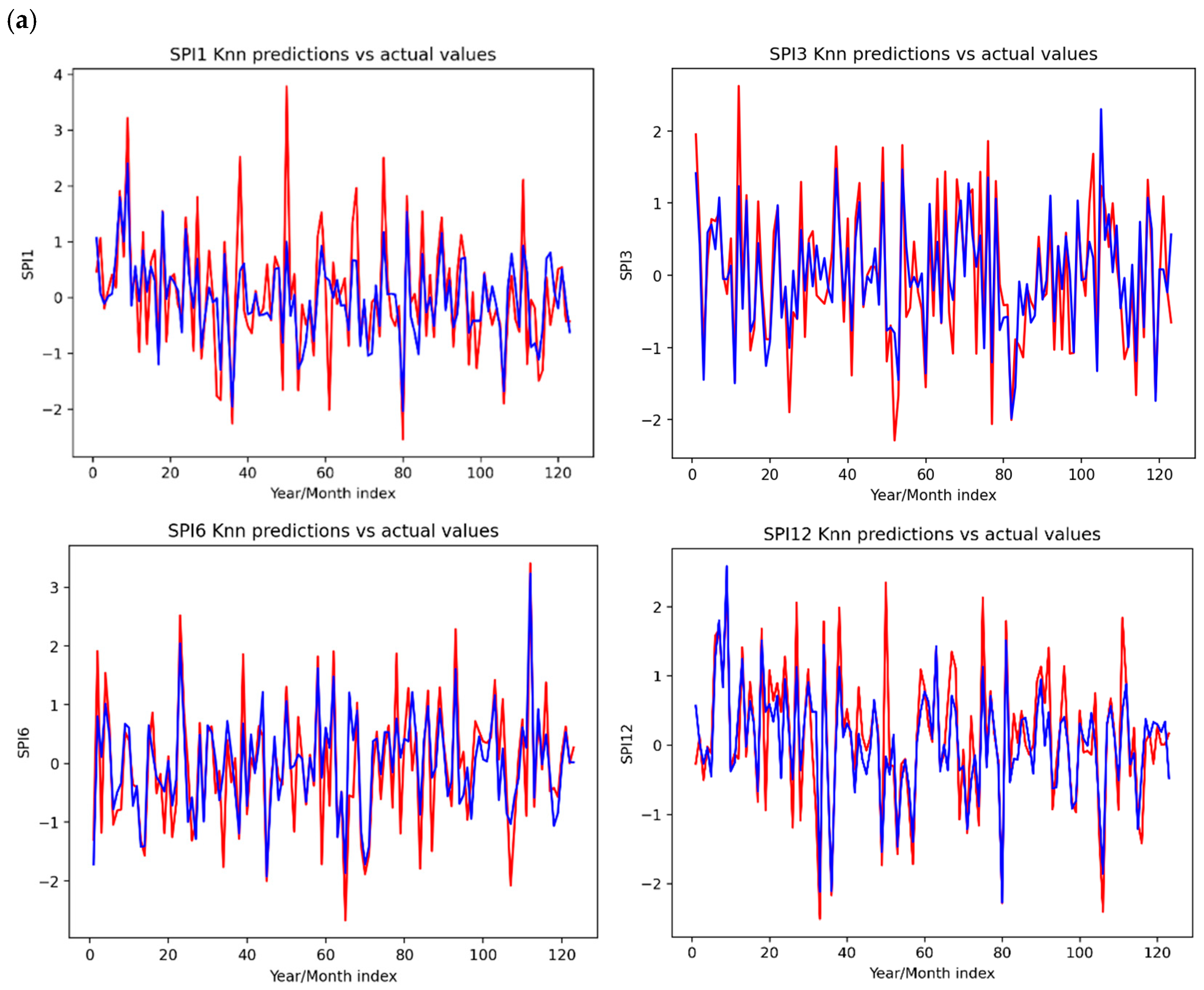
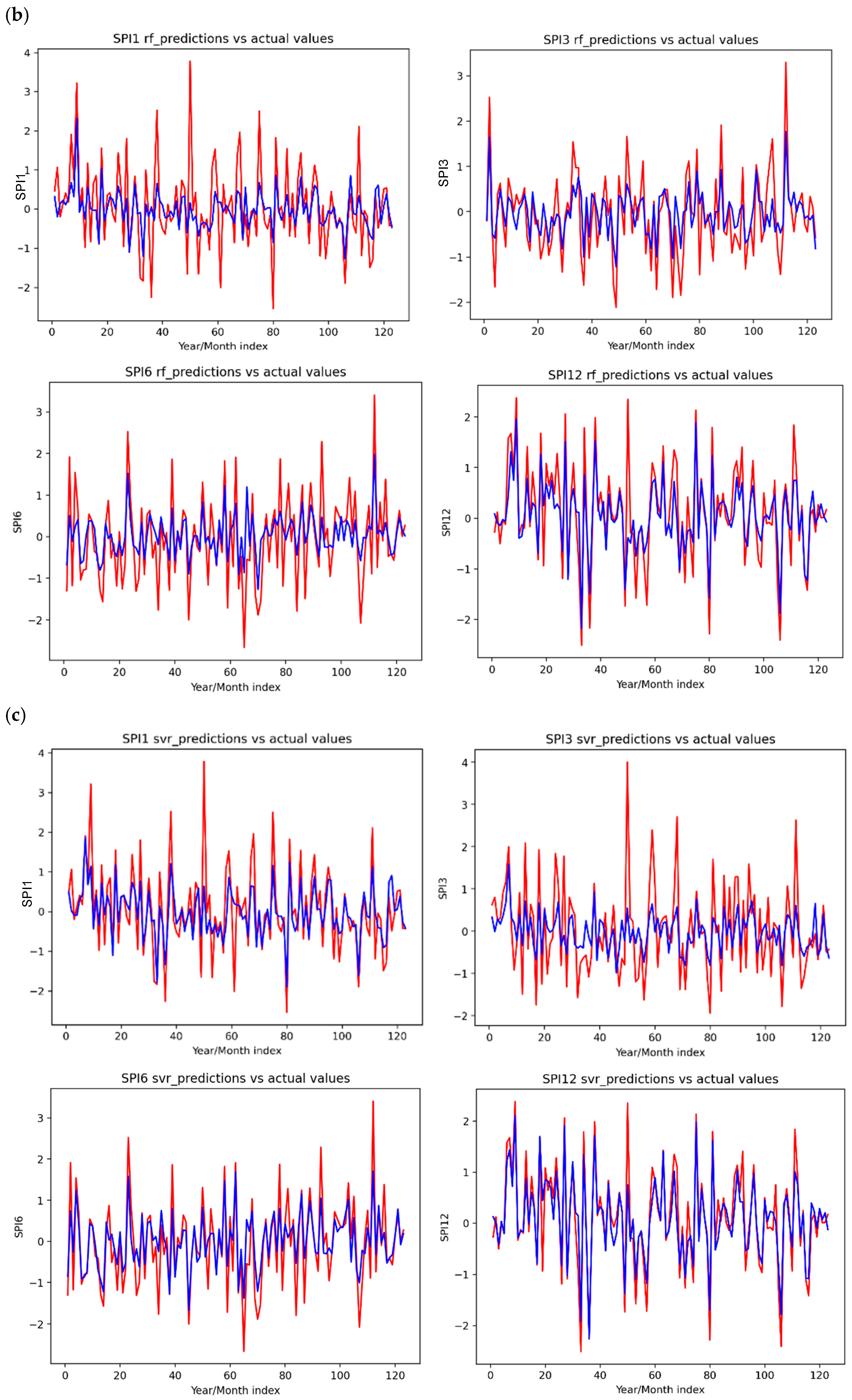
The prediction results (Figure 7) for the three different Standardized Precipitation Index (SPI) values (SPI_12, SPI_6, SPI_3, and SPI_1) are similar in terms of the evaluation metrics used, which are Root Mean Squared Error (RMSE), Mean Squared Error (MSE), Pearson Correlation Coefficient (r), and Coefficient of Determination (R²).

Figure 7. Line plot of observed (red) vs. estimated (blue) SPI values by the (a) k-Nearest Neighbor, (b) Random Forest, (c) Support Vector Machine at Sfax station for SPI-1, SPI-3, SPI-6, SPI-12.

In general, the results show that the SVR model has a high performance in predicting drought using the SPI values, with all four evaluation metrics indicating a good fit between the predicted and actual drought values.

For the SPI_6, the RMSE and MSE values are 0.37 and 0.14, respectively, which indicates that the average difference between the observed and predicted values is small. The correlation coefficient (r) is 0.84, which is close to 1, indicating a strong positive correlation between the observed and predicted values. The R² value is 0.65, indicating that 65% of the variation in the observed values can be explained by the model.

For the SPI_3, the RMSE and MSE values indicate that the average difference between the observed and predicted values is small. The correlation coefficient (r) varies between 0.71 and 0.81, indicating a strong positive correlation between the observed and predicted values. The R2 value varies between 0.43 and 0.67, indicating that most of the variation in the observed values can be explained by the model.

For the SPI_12, the performance of the models (SVR, RF, kNN) was found to be lower in comparison to the shorter timescales. The RMSE and MSE values indicate a higher average difference between observed and predicted values, reflecting the greater difficulty in accurately predicting drought over a longer accumulation period. The correlation coefficient (r) is moderate, ranging between 0.25 and 0.88, which suggests almost a weaker positive correlation between the observed and predicted values compared to SPI_1, SPI_3 and SPI_6. The R² value, ranging from 0.43 to 0.85, highlights the challenges in using SPI_12 as an input for drought prediction.

The SPI_1 values (Figure 7) demonstrate superior performance in terms of Root Mean Squared Error (RMSE) and Mean Squared Error (MSE), showing the lowest error between predicted and actual drought values among the three SPI indices. This is further supported by the high correlation coefficient (r) and coefficient of determination (R²) for all SPI values, which indicate a strong relationship between predicted and actual drought conditions.

In conclusion, the SPI values (SPI_12, SPI_6, and SPI_1) generally provide good predictive performance for the Support Vector Regression (SVR) model in drought forecasting, with SPI_1 exhibiting the best performance. While SPI values effectively capture the cyclical behaviour of precipitation over short timescales, they fall short in explicitly defining drought events. For understanding broader patterns, such as persistent dry and wet cycles, the longer timescale SPI values (e.g., SPI-12) prove more insightful, aligning with the findings of De Jesus et al. (2016) [49].

The Support Vector Regression (SVR) model demonstrated superior predictive accuracy in our study due to its specific architectural advantages in handling the multivariate, non-stationary nature of hydroclimatic drought signals. Unlike simpler linear models, SVR—with a carefully optimized Radial Basis Function (RBF) kernel—was able to project the complex interactions between our core predictors (SPI-1, SPI-3, SPI-6, SPI-12) into a high-dimensional feature space where non-linear relationships become linearly separable.

The forecasting results from the three models used in this study show valuable outcomes with strong correlation coefficients. Notably, the SPI-12 input variable achieved an improved performance, reaching a coefficient of determination (R²) of 0.85. Our findings are consistent with Ben Abdelmalek et al. (2020) [51], who identified a cyclical pattern of drought occurrences, typically alternating every 3 to 7 years. This cyclical behaviour is reflected in our results, demonstrating a consistent frequency and duration of drought periods over the study period.

This research highlights the utility of the Standardized Precipitation Index (SPI) in drought monitoring while acknowledging its limitations. Although SPI is a valuable tool, it relies solely on precipitation data, neglecting other crucial climate variables. As a result, it provides an incomplete view of drought dynamics, limiting insights into the onset and termination of drought periods and reducing its effectiveness in timely drought management. To mitigate these limitations, future research should incorporate additional climate variables and geographical factors to enhance accuracy. Such improvements would strengthen drought forecasting capabilities and contribute to a more comprehensive approach to drought management. Furthermore, the study’s use of a dataset spanning over 100 years adds robustness to the analysis and forecasting efforts.

An analysis of model prediction errors over the testing period (1998–2017) revealed a degree of temporal instability. While overall performance metrics were consistent, the models exhibited higher error variance during periods of extreme drought (severely negative SPI) and extreme wetness (high positive SPI). This indicates that the models are more reliable for predicting conditions within the near-normal to moderate drought range, while their accuracy diminishes for classifying the tails of the distribution, where hydrological impacts are often most acute. Furthermore, no systematic increase in error was observed throughout the testing period, suggesting the models did not experience significant performance decay within the 20-year validation window.

The findings of this study reveal clear seasonal and long-term drought patterns in Sfax, supported by increasing SPI dryness trends that are consistent with results reported in similar Mediterranean semi-arid regions [23,38]. The performance of the model aligns with previous studies emphasizing the importance of long-term rainfall records and reliable climate data [45,53,54]. Some limitations remain, including missing values and uncertainties in extreme rainfall events, but the method still provides useful insight into drought evolution and its potential impacts on agriculture and groundwater stress. As also noted in related research [28,41], the proposed approach is transferable to other arid regions and can be improved by integrating additional climate variables and higher-resolution datasets.

Regarding future applicability, the stability of model performance is contingent upon the stationarity of the climate system. The identified long-term, statistically significant trends in SPI-18 and SPI-24 (Table 3) signal an evolving hydrological baseline. If these trends persist or accelerate due to climate change, the models—trained on a historical dataset that may not fully represent future conditions—are likely to experience performance degradation over time. To ensure ongoing reliability, we recommend periodic retraining of the models with recent data and the future incorporation of climate indices (e.g., NAO, ENSO) or outputs from global climate models as predictors to better account for low-frequency climate oscillations and long-term anthropogenic trends.

6. Conclusions

The computed Standardized Precipitation Index (SPI) values consistently demonstrate a high level of reliability throughout both wet and dry periods across various time scales. Notably, we observe a diminishing amplitude of fluctuations as the time scale increases.

This study highlights the remarkable effectiveness of Support Vector Regression (SVR) and k-Nearest Neighbor (kNN) models in the domain of meteorological drought prediction. Specifically, the SVR approach excels across most of the employed SPIs (i.e., SPI1, SPI6, SPI12), proficiently capturing temporal drought patterns. It achieves a notable coefficient of determination (R² = 0.85) and exhibits commendable performance in residual predictive deviation.

Our research emphasizes the consistency of utilizing SPI, particularly in conjunction with Support Vector Regression, for predicting drought occurrences and assessing their severity in the near future. This capability holds significant promise for local communities, enabling them to tailor land-use strategies and proactively devise approaches to mitigate impending drought challenges.

In summary, this study adeptly addresses the challenge of incomplete historical data in monitoring and forecasting regional drought events. This accomplishment is underscored by the strategic use of advanced data imputation techniques, the integration of ensemble learning methodologies, and the application of robust machine learning models, including Support Vector Machines (SVM), among others.

These findings improve our understanding of drought dynamics in Sfax and provide practical guidance for developing early-warning and risk-management strategies. The machine learning models used here offer a solid basis for predicting monthly drought conditions and supporting more informed decisions in water and agricultural planning.

Future work could extend this approach to other regions and integrate additional variables such as soil moisture and temperature to enrich model performance. The use of deep learning methods—such as LSTM or transformer-based models—also presents a promising direction for capturing complex temporal patterns and further improving drought prediction accuracy.

References

1. Carter, R.; Parker, A. Climate change, population trends, and groundwater in Africa. Hydrol. Sci. J. 2009, 54, 676–689. [Google Scholar] [CrossRef]
2. Dai, A. Drought under global warming: A review. Wiley Interdiscip. Rev. Clim. Change 2010, 1, 45–56, Erratum in Wiley Interdiscip. Rev. Clim. Change 2012, 3, 617. [Google Scholar] [CrossRef]
3. Mckee, T.B.; Doesken, N.J.; Kleist, J. The relationship of drought frequency and duration to timescales. In Proceedings of the 8th Conference on Applied Climatology, Anaheim, CA, USA, 17–22 January 1993; pp. 179–184. [Google Scholar]
4. Hayes, M.; Svoboda, M.; Wall, N.; Widhalm, M. The Lincoln declaration on drought indices: Universal meteorological drought index recommended. Bull. Am. Meteorol. Soc. 2011, 92, 485–488. [Google Scholar] [CrossRef]
5. Liu, Z.N.; Li, Q.F.; Nguyen, L.B.; Xu, G.H. Comparing Machine-Learning Models for Drought Forecasting in Vietnam’s Cai River Basin. Pol. J. Environ. Stud. 2018, 27, 2633–2646. [Google Scholar] [CrossRef]
6. Nguyen, L.B.; Li, Q.F.; Ngoc, T.A.; Hiramatsu, K. Adaptive Neuro–Fuzzy Inference System for Drought Forecasting in the Cai River Basin in Vietnam. J. Fac. Agric. Kyushu Univ. 2015, 60, 405. [Google Scholar] [CrossRef]
7. Wei, S.; Zuo, D.; Song, J. Improving prediction accuracy of river discharge time series using a Wavelet-NAR artificial neural network. J. Hydroinform. 2012, 14, 974. [Google Scholar] [CrossRef]
8. Abbot, J.; Marohasy, J. Application of artificial neural networks to rainfall forecasting in Queensland, Australia. Adv. Atmos. Sci. 2012, 29, 717–730. [Google Scholar] [CrossRef]
9. Abbot, J.; Marohasy, J. Input selection and optimization for monthly rainfall forecasting in Queensland, Australia, using artificial neural networks. Atmos. Res. 2014, 138, 166–178. [Google Scholar] [CrossRef]
10. Şahin, M.; Kaya, Y.; Uyar, M.; Yıldırım, S. Application of extreme learning machine for estimating solar radiation from satellite data. Int. J. Energy Res. 2014, 38, 205–212. [Google Scholar] [CrossRef]
11. Govindaraju, R.S. Artificial neural networks in hydrology. II: Hydrologic applications. J. Hydrol. Eng. 2000, 5, 124–137. [Google Scholar]
12. Gacu, J.G.; Monjardin, C.E.F.; Mangulabnan, R.G.T.; Pugat, G.C.E.; Solmerin, J.G. Artificial Intelligence (AI) in Surface Water Management: A Comprehensive Review of Methods, Applications, and Challenges. Water 2025, 17, 1707. [Google Scholar] [CrossRef]
13. Rathore, W.U.A.; Ni, J.; Ke, C.; Xie, Y. BloomSense: Integrating Automated Buoy Systems and AI to Monitor and Predict Harmful Algal Blooms. Water 2025, 17, 1691. [Google Scholar] [CrossRef]
14. Masinde, M. Artificial neural networks models for predicting effective drought index: Factoring effects of rainfall variability. Mitig. Adapt. Strateg. Glob. Change 2013, 19, 1139–1162. [Google Scholar] [CrossRef]
15. Nastos, P.; Paliatsos, A.; Koukouletsos, K.; Larissi, I.; Moustris, K. Artificial neural networks modeling for forecasting the maximum daily total precipitation at Athens, Greece. Atmos. Res. 2014, 144, 141–150. [Google Scholar] [CrossRef]
16. Acharya, N.; Shrivastava, N.A.; Panigrahi, B.; Mohanty, U. Development of an artificial neural network based multi-model ensemble to estimate the northeast monsoon rainfall over south peninsular India: An application of extreme learning machine. Clim. Dyn. 2013, 43, 1303–1310. [Google Scholar] [CrossRef]
17. Jain, V.K.; Pandey, R.P.; Jain, M.K.; Byun, H.R. Comparison of drought indices for appraisal of drought characteristics in the Ken River Basin. Weather Clim. Extrem. 2015, 8, 1–11. [Google Scholar] [CrossRef]
18. Mondol, M.A.H.; Ara, I.; Das, S.C. Meteorological drought index mapping in Bangladesh using Standardized Precipitation Index during 1981–2010. Adv. Meteorol. 2017, 2017, 4642060. [Google Scholar] [CrossRef]
19. Gallear, J.W.; Valadares Galdos, M.; Zeri, M.; Hartley, A. Evaluation of machine learning approaches for large-scale agricultural drought forecasts to improve monitoring and preparedness in Brazil. Nat. Hazards Earth Syst. Sci. 2025, 25, 1521–1541. [Google Scholar] [CrossRef]
20. Gyaneshwar, A.; Mishra, A.; Chadha, U.; Raj Vincent, P.M.D.; Rajinikanth, V.; Pattukandan Ganapathy, G.; Srinivasan, K. A Contemporary Review on Deep Learning Models for Drought Prediction. Sustainability 2023, 15, 6160. [Google Scholar] [CrossRef]
21. Nandgude, N.; Singh, T.P.; Nandgude, S.; Tiwari, M. Drought Prediction: A Comprehensive Review of Different Drought Prediction Models and Adopted Technologies. Sustainability 2023, 15, 11684. [Google Scholar] [CrossRef]
22. Moore, I.D.; Grayson, R.B.; Ladson, A.R. Digital Terrain Modelling: A Review of Hydrological, Geomorphological, and Biological Applications. Hydrol. Process. 1991, 5, 3–30. [Google Scholar] [CrossRef]
23. Li, M.; Yao, Y.; Feng, Z.; Ou, M. Hydrological drought prediction and its influencing features analysis based on a machine learning model. Nat. Hazards Earth Syst. Sci. 2025, 25, 4299–4316. [Google Scholar] [CrossRef]
24. Liu, R.; Yin, J.; Slater, L.; Kang, S.; Yang, Y.; Liu, P.; Guo, J.; Gu, X.; Zhang, X.; Volchak, A. Machine-learning-constrained projection of bivariate hydrological drought magnitudes and socioeconomic risks over China. Hydrol. Earth Syst. Sci. 2024, 28, 3305–3326. [Google Scholar] [CrossRef]
25. Giri, A.; Chakraborty, J. Analysis of machine learning algorithms in drought prediction. Comput. Res. Dev. 2023, 23, 52–71. [Google Scholar]
26. Tan, X.; Zhao, Q.; Liu, Y.; Zhang, X. DroughtSet: Understanding Drought Through Spatial-Temporal Learning. arXiv 2024, arXiv:2412.15075. [Google Scholar] [CrossRef]
27. Mansour, M.; Habaieb, H. Agro-climatic characterization of the Sfax region based on long-term observations from the Ezzitouna station. Tunis. J. Agric. Sci. 2016, 34, 112–125. [Google Scholar]
28. Lazcano, A. Walking back the data quantity assumption to improve time series forecasting. Appl. Sci. 2024, 14, 11081. [Google Scholar] [CrossRef]
29. Patel, N.R.; Chopra, P.; Dadhwal, V.K. Analyzing spatial patterns of meteorological drought using standardized precipitation index. Meteorol. Appl. 2007, 14, 329–336. [Google Scholar] [CrossRef]
30. McRoberts, D.B.; Nielsen-Gammon, J.W. The use of a high-resolution standardized precipitation index for drought monitoring and assessment. J. Appl. Meteorol. Climatol. 2012, 51, 68–83. [Google Scholar] [CrossRef]
31. Chen, S.; Zhang, L.; Zhang, Y.; Guo, M.; Liu, X. Evaluation of Tropical Rainfall Measuring Mission (TRMM) satellite precipitation products for drought monitoring over the middle and lower reaches of the Yangtze. J. Geogr. Sci. 2020, 30, 53–67. [Google Scholar] [CrossRef]
32. Santos, J.F.; de Sentous, P.J.G.M.; Blain, G.C. Standardized Precipitation Index (SPI) calculation using the incomplete gamma distribution function: Monthly rainfall fitting, gamma-distribution parameters and transformation to a standard normal variable. J. Geogr. Sci. 2017, 30, 53–67. [Google Scholar]
33. McKee, T.B. Drought monitoring with multiple time scales. In Proceedings of the 9th Conference on Applied Climatology, Dallas, TX, USA, 15–20 January 1995. [Google Scholar]
34. Breiman, L. Bagging Predictors. Mach. Learn. 1996, 24, 123–140. [Google Scholar] [CrossRef]
35. Bacanli, U.; Firat, M.; Dikbas, F. Adaptive Neuro-Fuzzy Inference System for drought forecasting. Stoch. Environ. Res. Risk Assess. 2009, 23, 1143. [Google Scholar] [CrossRef]
36. Hyndman, R.J.; Athanasopoulos, G. Forecasting: Principles and Practice, 2nd ed.; OTexts: Melbourne, Australia, 2018; ISBN 978-0987507112. [Google Scholar]
37. Deo, R.C.; Şahin, M. Application of the extreme learning machine algorithm for the prediction of monthly Effective Drought Index in eastern Australia. Atmos. Res. 2015, 153, 512–525. [Google Scholar] [CrossRef]
38. Achite, M.; Elshaboury, N.; Jehanzaib, M.; Vishwakarma, D.K.; Pham, Q.B.; Anh, D.T.; Abdelkader, E.M.; Elbeltagi, A. Performance of Machine Learning Techniques for Meteorological Drought Forecasting in the Wadi Mina Basin, Algeria. Water 2023, 15, 765. [Google Scholar] [CrossRef]
39. Vapnik, V.N. The Nature of Statistical Learning Theory, 2nd ed.; Springer: New York, NY, USA, 1999. [Google Scholar]
40. Dibike, Y.B.; Coulibaly, P.; Anctil, F. Comparison of Support Vector Machines and Neural Networks for the Prediction of Water Levels in the Mackenzie River. J. Hydrol. 2001, 253, 55–70. [Google Scholar]
41. Smola, A.J.; Schölkopf, B. A Tutorial on Support Vector Regression. Stat. Comput. 2004, 14, 199–222. [Google Scholar] [CrossRef]
42. Loukas, A.; Vasiliades, L. Probabilistic analysis of drought spatiotemporal characteristics in Thessaly region, Greece. Nat. Hazards Earth Syst. Sci. 2004, 4, 719–731. [Google Scholar] [CrossRef]
43. Cover, T.M.; Hart, P.E. Nearest neighbor pattern classification. IEEE Trans. Inf. Theory 1967, 13, 21–27. [Google Scholar] [CrossRef]
44. Yakowitz, S. Nearest-neighbor methods for time series, with applications to rainfall/runoff prediction. J. Time Ser. Anal. 1987, 8, 235–247. [Google Scholar] [CrossRef]
45. Karlsson, M. Nearest-neighbor methods for nonparametric rainfall-runoff modeling. Water Resour. Res. 1987, 23, 1300–1308. [Google Scholar] [CrossRef]
46. Lall, U.; Sharma, A. A nearest neighbor bootstrap for resampling hydrologic time series. Water Resour. Res. 1996, 32, 679–693. [Google Scholar] [CrossRef]
47. Tan, M.L.; Tan, K.C.; Chua, V.P.; Chan, N.W. Evaluation of TRMM Product for Monitoring Drought in the Kelantan River Basin, Malaysia. Water 2017, 9, 57. [Google Scholar] [CrossRef]
48. Nabaei, S.; Sharafati, A.; Yaseen, Z.M.; Shahid, S. Copula based assessment of meteorological drought characteristics: Regional investigation of Iran. Agric. For. Meteorol. 2019, 276, 107611. [Google Scholar] [CrossRef]
49. De Jesus, J.M.; Silva, A.R.; Rodrigues, M.A. A machine learning model for drought tracking and forecasting using satellite-based precipitation data. Environ. Model. Softw. 2016, 86, 1–12. [Google Scholar]
50. Feng, Y.; Cui, N.; Gong, D.; Zhang, Q.; Zhao, L. Evaluation of random forests and generalized regression neural networks for daily reference evapotranspiration modelling. Agric. Water Manag. 2020, 227, 117834. [Google Scholar] [CrossRef]
51. Ben Abdelmalek, M.; Nouiri, I. Study of trends and mapping of drought events in Tunisia and their impacts on agricultural production. Sci. Total Environ. 2020, 734, 139311. [Google Scholar] [CrossRef] [PubMed]
52. Bouaziz, M.; Medhioub, E.; Csaplovisc, E. A machine learning model for drought tracking and forecasting using remote precipitation data and a standardized precipitation index from arid regions. J. Arid Environ. 2021, 189, 104478. [Google Scholar] [CrossRef]
53. Mandal, I.; Pal, S. Modelling human health vulnerability using different machine learning algorithms in stone quarrying and crushing areas of Dwarka river Basin. Adv. Space Res. 2020, 66, 1351–1371. [Google Scholar] [CrossRef]
54. Kendall, M.G. Rank Correlation Methods; Charles Griffin: London, UK, 1975. [Google Scholar]
Disclaimer/Publisher’s Note: The statements, opinions and data contained in all publications are solely those of the individual author(s) and contributor(s) and not of MDPI and/or the editor(s). MDPI and/or the editor(s) disclaim responsibility for any injury to people or property resulting from any ideas, methods, instructions or products referred to in the content.
Article Metrics
Citations
Article Access Statistics
Multiple requests from the same IP address are counted as one view.