Article

Integrating UAV-LiDAR and Field Experiments to Survey Soil Erosion Drivers in Citrus Orchards Using an Exploratory Machine Learning Approach

by
Jesús Rodrigo-Comino
1,2,*,
Laura Cambronero-Ruiz
1,2,
Lucía Moreno-Cuenca
1,2,
Jesús González-Vivar
1,
María Teresa González-Moreno
1,2,3 and
Víctor Rodríguez-Galiano
4
1
Departamento de Análisis Geográfico Regional y Geografía Física, Facultad de Filosofía y Letras, Campus Universitario de Cartuja, University of Granada, 18071 Granada, Spain
2
Andalusian Research Institute in Data Science and Computational Intelligence, University of Granada, 18016 Granada, Spain
3
Medialab UGR—Research Laboratory for Digital Culture and Society, University of Granada, 18016 Granada, Spain
4
Departamento de Geografía Física y Análisis Geográfico Regional, Universidad de Sevilla, 41004 Seville, Spain
*
Author to whom correspondence should be addressed.
Water 2025, 17(24), 3541; https://doi.org/10.3390/w17243541
Submission received: 22 October 2025 / Revised: 10 December 2025 / Accepted: 11 December 2025 / Published: 14 December 2025

Abstract

Citrus orchards are especially vulnerable owing to low inter-row vegetation cover, and frequent tillage. Here, we combine controlled field experiments with proximal remote sensing–derived geomorphometric variables and machine learning (ML) to identify key factors of erosion in a Mediterranean climate citrus plantation located close to Seville and the National Park of Doñana (Southern Spain) on Gleyic Regosols (clayic, arenic). We conducted rainfall simulations with 30 s sampling, measured infiltration (mini-disc infiltrometer), saturated hydraulic conductivity (Kfs; Guelph permeameter), compaction (penetrologger), and soil respiration (gas analyzer) at multiple points, and derived high resolution morphometric indices from proximal sensing (UAV-LiDAR). Linear models and Random Forests were trained to explain three responses: soil loss, sediment concentration (SC), and runoff. Results show that soil loss is most strongly associated with maximum compaction and Kfs (multiple regression: R2 = 0.68; adjusted R2 = 0.52; p = 0.063), while SC increases with surface compaction and exhibits weak relationships with topographic metrics. Runoff decreases with average infiltration, which is related to compaction (β = −4.83 ± 2.38; R2 = 0.34; p = 0.077). Diagnostic checks indicate centered residuals with mild heteroscedasticity and a few high leverage observations. Random Forests captured part of the variance for soil loss (≈29%) but performed poorly for runoff, consistent with limited sample size and modest nonlinear signal. Morphometric analysis revealed gentle relief but pronounced convergent–divergent patterns that modulate hydrological connectivity. There were strong differences in the experiments conducted close to the trees and in the tractor trails. We conclude that compaction and near surface hydraulic properties are the most influential and measurable controls of erosion at plot scale and the UAV-LiDAR could not give us extra-insights. We highlight that integrating standardized field protocols with proximal morphometrics and ML can be the best method to prioritize a small set of explanatory variables, helping to reduce experimental effort while maintaining explanatory power.

1. Introduction

Soil erosion and land degradation are among the most pressing environmental challenges of the 21st century, particularly in the context of accelerating climate change, intensive land use, and resource depletion [1,2]. Climate projections suggest that the frequency and intensity of extreme rainfall events will increase in many regions, exacerbating soil erosion and the associated loss of soil fertility, water storage capacity, and ecosystem services (IPCC, 2022; https://www.ipcc.ch). Unsustainable agricultural practices, especially those characterized by intensive soil management, further aggravate these processes as demonstrated many years ago [3,4]. However, this has resulted in widespread topsoil depletion, declining crop productivity, and deterioration of water quality [5,6,7]. Tackling soil erosion is therefore critical to achieving both global food security and sustainable land management, as the degradation of arable land directly threatens the resilience of agricultural systems [8,9].
In perennial cropping systems such as citrus orchards, soil erosion rates are particularly severe due to sloping terrain, frequent tillage, and low ground cover between rows [10,11,12]. This issue has severe economic and environmental consequences, especially in major citrus-producing regions [13]. For example, studies in China in citrus have reported soil loss rates exceeding tolerable thresholds by up to several times [14,15], while research in Spain has highlighted high sediment yields and off-site impacts in Mediterranean orchards under conventional management [16]. Similarly, in South America, citrus plantations in countries such as Brazil show significant rates of soil and nutrient loss, which compromise soil fertility and water quality downstream [17,18]. These examples illustrate that soil erosion in perennial orchards is a global problem with direct implications for agricultural sustainability and ecosystem services.
Addressing this challenge effectively requires robust and reliable field data. High-quality datasets with sufficient replication, standardized equipment, and reproducible protocols are essential for quantifying soil erosion processes and for calibrating and validating predictive models [19,20,21]. Experimental approaches such as rainfall simulation experiments, infiltration and permeability measurements, and soil compaction assessments provide crucial insights into the physical mechanisms driving erosion [22,23]. However, these techniques are labor-intensive, time-consuming, and often restricted to small spatial scales, which limits their broader applicability, especially as a nature-based solutions [24,25].
Recent advances in machine learning (ML) offer an opportunity to overcome some of these limitations by detecting patterns and predicting soil erosion risks from complex datasets [26]. While ML applications have become increasingly common in soil science, the integration of proximal remote sensing data such as drones—which allows the derivation of high-resolution geomorphological and morphometric information [27,28]—with field experiments remains rare. Traditionally, methodologies such as rainfall simulation experiments, infiltration and compaction measurements, or soil respiration analysis have been applied independently, without linking them to spatially explicit datasets. The main novelty of our article is the integration of a specific approach at the same time, which enables the identification of the key explanatory factors behind soil erosion from multiple perspectives, thereby reducing the number of experiments and variables required and improving the scalability and cost-effectiveness of monitoring programs. The new results would be related to the identification of the most influential explanatory factors controlling soil loss and sediment dynamics in woody crop systems, thereby improving the design of soil erosion monitoring strategies and reducing the need for extensive experimental campaigns.
In this study, our main novelty and primary objective is to combine controlled field experiments with proximal remote sensing-derived morphometric variables to better understand soil erosion dynamics in citrus orchards. We conducted a series of rainfall simulation experiments, infiltration, permeability, compaction, and soil respiration measurements at multiple sampling points (10), which were then integrated with detailed geomorphometric information derived from proximal sensing (UAV-LiDAR) using machine learning algorithms to detect patterns and relationships.
Our working hypothesis is that integrating standardized field experiments with proximal remote sensing-derived geomorphometric data through machine learning would allow the detection of a small subset of explanatory variables that account for most of the observed variability in soil erosion. If confirmed, this approach could substantially optimize the monitoring process by minimizing the number of field experiments required, improving the spatial extrapolation of results to larger areas, and providing a cost-effective framework for sustainable soil management in citrus orchards worldwide.

2. Materials and Methods

2.1. Study Area Description

The study was conducted in a commercial citrus orchard located in the province of Seville (southern Spain; Figure 1a), in proximity to the Doñana National Park, a region characterized by its Mediterranean agroecosystem and flat topography. The selected site lies on tow inter-row lines with minimal slope (<5%; Figure 1b) and an elevation of approximately 5.4 m above sea level (Figure 1c). The orchard is cultivated with orange trees under irrigated conditions for most of the year due to very poor natural drainage and twice tilled per year using heavy machinery. Soil sampling and field experiments were carried out near the coordinates 209599.5 E, 4119656.5 N (EPSG:25830; UTM Zone 30N). The experimental orchards were planted in April 2010 in the Lower Guadalquivir Valley and comprise four citrus varieties: Navel Powell and Barnfield (both grafted onto Carrizo citrange), Nova (Citrumelo rootstock), and Valencia Midknight (Macrophylla rootstock). All plots share the same planting frame (7 m × 4 m), tree age (15.7 years), and similar management practices, including drip irrigation, annual tillage, and chemical weed control. This homogeneity ensured consistency across the experimental conditions while allowing for comparison across scion–rootstock combinations.
The soil at the site is classified as a Gleyic Regosol (clayic, arenic) according to the IUSS-WRB [29] classification system (Figure 1d). It developed from a heterogeneous mix of silt, sand, and clay, with surface compaction observable in tractor traffic lanes and lower horizons, though no surface sealing was detected. The surface horizon (A) shows a silty clay loam texture, moderate blocky and prismatic structure, and ferric mottling indicating hydromorphic processes. Subsurface horizons (B and B/C) are compact, with low biological activity and poor aggregation stability (0.18–0.25), high pH values (7.89–7.99), and low to moderate electrical conductivity (421–462 μS/cm). The orchard exhibits signs of surface erosion, particularly between the rows on slight mounds, and features wide desiccation cracks (2–5 cm width, up to 20 cm deep). Rock outcrops are absent, and coarse fragments are scarce (<10%), which, together with the weak aggregation and high compaction, suggest vulnerability to both waterlogging and erosion. The site’s accessibility and contrasting microtopographic features made it suitable for the installation of rainfall simulation plots, infiltration tests, and soil physical and biological monitoring. The Bajo Guadalquivir region, located in southwestern Andalusia (Spain), experiences a Mediterranean sub-humid to semi-arid climate, characterized by hot, dry summers and mild, wet winters. According to the Junta de Andalucía’s climate classification (https://www.juntadeandalucia.es/medioambiente/portal/areas-tematicas/cambio-climatico-y-clima/clima-en-andalucia/regiones-climaticas-de-andalucia, accessed on 10 December 2025), the area is characterized by mean annual temperatures between 17 °C and 19 °C, with maximum summer temperatures often exceeding 40 °C, especially in July and August. Annual precipitation ranges from 500 to 700 mm, distributed irregularly across the year and concentrated in autumn and winter months (October–March). The prolonged dry season, combined with intense rainfall episodes, increases the vulnerability of the soil to erosion processes. This climatic regime exerts a strong influence on hydrological dynamics and vegetation cover, with important implications for runoff generation, infiltration patterns, and the intensity of erosive processes in cultivated lands such as citrus orchards.

2.2. UAV-Based Photogrammetry, Field Experiments and Laboratory Analysis

Due to the logistical complexity of conducting rainfall simulations and in-situ soil measurements across a working commercial citrus plantation, we opted for a high-replication, low-spatial-extent sampling design. Each sampling point was selected to represent a distinct morphometric unit derived from proximal sensing data, and field measurements were repeated per point using standardized protocols. The average values of these replicates were used to characterize each point (Supplementary Material S1). While this approach limits the number of spatial units (n = 10), it enhances internal consistency and minimizes intra-plot variability because they were carried out the same days. This trade-off is not common in soil erosion studies under real-field conditions because the necessity of joining various trained researchers and specific calibrated devices the same days at the same moment, also where physical constraints restrict the number of simulated rainfall events that can be realistically deployed.

2.2.1. UAV Survey and LiDAR Data Acquisition Workflow

Ground Control Points (GCPs) were strategically placed throughout the site using a high-precision GNSS receiver (Leica Zeno 20; Leica Geosystems, Heerbrug, Switzerland), with centimeter-level accuracy). The UAV platform employed in this study was a DJI Matrice 350 RTK (Shenzhen, China) equipped with a LiDAR sensor. This quadcopter features a Real-Time Kinematic (RTK) positioning system, enabling real-time, high-accuracy georeferencing. The onboard sensor, a DJI Zenmuse L2 (Shenzhen, China), integrates LiDAR technology with a high-resolution RGB camera. The onboard RGB camera delivered 20 MP resolution, enabling point cloud colorization. The mission comprised three flights conducted at mean altitudes of 51.9 m, 56.5 m, and 77.8 m, with average flight speeds between 4.1 and 4.2 m/s. Processing in DJI Terra, set to high point density (100%), produced point clouds with an average density of 1702 points/m2 across the study area (0.378 km2), from which a digital elevation model (DEM) was generated at 0.1 m/pixel resolution.
This setup allows for the generation of high-density 3D point clouds, which are crucial for detailed topographic reconstruction, detection of vegetation cover changes, and the production of digital terrain and surface models. The acquired data were processed using DJI Terra software (V.5) and subsequently analyzed and visualized through Geographic Information System (GIS) tools (ArcGIS Pro (https://www.esri.com/en-us/arcgis/products/arcgis-pro/overview, accessed on 10 December 2025), ESRI, Louisville, CO, USA). In the case of LiDAR data, the processed outputs included 3D point clouds and both Digital Surface Models (DSM) and Digital Terrain Models (DTM). For DSM and DTM products derived from LiDAR, a Canopy Height Model (CHM) was computed by subtracting the DTM from the DSM. This allowed estimation of vegetation height at each sampling location. However, since the sampling points were deliberately placed in bare inter-row areas free of canopy cover, the CHM was only used as a verification layer and not included in the predictive analysis. Vegetation density was not computed from LiDAR data; field observations and imagery were used to confirm the absence of vegetative obstruction. Raster values for all morphometric indices were extracted using a 3 × 3 pixel window (equivalent to ~1.8 m2), centered on each sampling point. This window size balances spatial precision with the need to reduce noise from microtopographic variability and positional uncertainty between UAV-derived rasters and GNSS-located field samples.
A total of 12 morphometric and topographic variables were derived from the high-resolution LiDAR-based Digital Elevation Model (DEM) using SAGA GIS (SAGA User Group/Hamburg University of Technology; Germany). The parameters include both average values and their corresponding standard deviations to capture the spatial heterogeneity within the sampling window. Specifically, slope characteristics were represented by Slope_mean and Slope_std, while curvature metrics included both Plan_Curvature and Profile_Curvature, providing insights into flow direction and profile convexity, respectively. Hydrological and catchment properties were described using Channel_Network_Base_Level, Channel_Network_Distance, Total_Catchment_Area, and the Topographic Wetness Index (TWI), all expressed as both mean and standard deviation values. Additional descriptors such as Aspect, Hillshade, LS Factor (from the RUSLE model), CIT (connectivity Index; adapted from [30]), and Convergence Index were also extracted to reflect solar radiation, erosive potential, flow accumulation, and network initiation thresholds. The inclusion of standard deviation values enhances the dataset’s capability to represent microtopographic heterogeneity, a critical factor in runoff generation and erosion processes. Finally, to extract local terrain attributes around each sampled point, a Python-based workflow was implemented using GeoPandas, Rasterio, and NumPy. A shapefile containing GPS-located citrus sampling points was reprojected to match the coordinate reference system (EPSG:25829) of the SAGA-derived raster layers. For each raster, mean and standard deviation values were extracted within a 3 × 3 pixel window centered on each point, effectively capturing microtopographic variability. The resulting values were compiled into a structured table and exported as a CSV file for subsequent statistical and machine learning analyses.

2.2.2. Rainfall Simulation Experiments

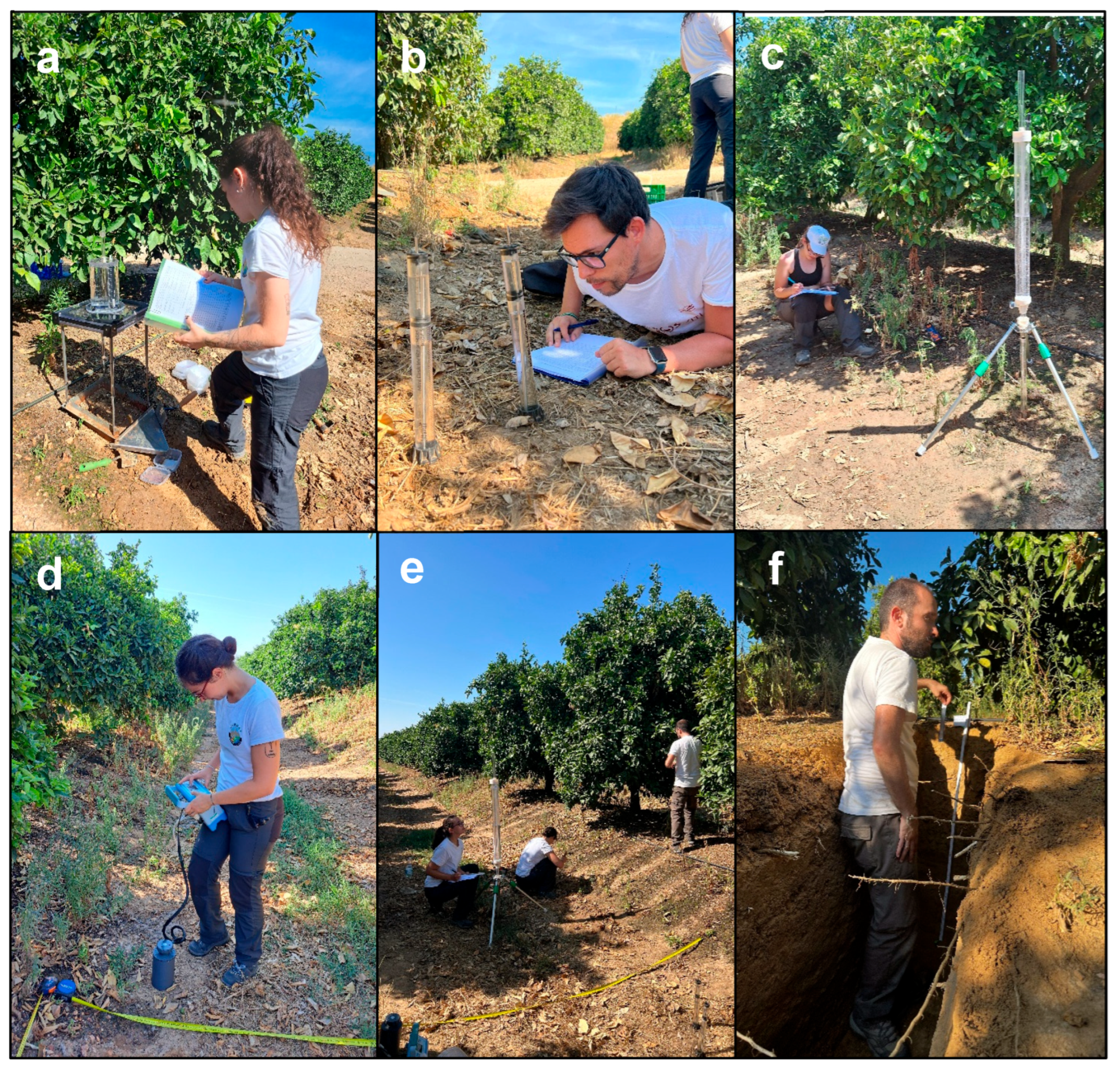
A total of ten rainfall simulation experiments were conducted to evaluate the response of the soil to controlled rainfall conditions, maintaining consistent parameters such as intensity, droplet size, water volume applied per unit area, and duration [31]. For this purpose, we used the mini-portable rainfall simulator developed by Eijkelkamp (The Netherlands), which applies artificial rainfall over a confined plot of 0.0625 m2 (Figure 2a). This device simulates rainfall through a pressurized sprinkler system, enabling the collection of quantitative data on runoff production, infiltration, and sediment detachment [32]. Although limited in spatial scale, the simulator is highly practical for field use due to its low water consumption, short setup time, and minimal personnel requirements [33]. It is particularly well-suited for estimating soil erodibility under standardized conditions, following methodologies such as those proposed by [34]. During each test, an identical volume of water was applied to each plot, and runoff and eroded sediment were collected through an outlet positioned at the base of the simulator. The simulated rainfall had a drop size of approximately 5.9 mm and was applied for 360 s at a steady rate of 6 mm·min−1. The equipment consists of three main components: a calibrated sprinkler head containing 49 capillary tubes to ensure uniform rainfall distribution; an adjustable aluminum stand to control drop height (maintained at 35–40 cm in our case); and a base frame to stabilize the system and direct water flow toward the outlet without lateral losses. Prior to each simulation, site-specific surface characteristics were recorded to assess their influence on runoff activation and erodibility [35,36]. These included: (i) vegetation cover (%), which was <5%, estimated through grid analysis of overhead photographs following (ii) rock fragment cover (%), also <5%, assessed using the same method; (iii) surface roughness, measured in both directions using the chain method described by [37]; and (iv) slope angle, determined with the LiDAR drone. During the simulation, the same operator—ensuring consistency and avoiding observer bias—recorded key hydrological response times: (i) Time to Ponding (Tp), indicating when the entire plot surface became visibly saturated; (ii) Time to Outlet (To), marking the appearance of the first drop at the outlet; and (iii) Time to Runoff Initiation (Tr), corresponding to the start of continuous surface flow [38]. After each experiment, the volume of runoff (liters) and sediment yield (grams) were determined in the laboratory. Runoff samples were evaporated at 110 °C to isolate solid content, and sediment concentration (g·L−1) was calculated by dividing the mass of solids by the volume of water collected.

2.2.3. Infiltration and Permeability Experiments

To evaluate soil permeability and infiltration capacity at the pedon scale (parallelly), two devices were employed at selected locations within the catchment area: a mini-disc infiltrometer (Figure 2b) and Guelph Permeameter (GP; Figure 2c). Simultaneously with the rainfall simulation experiments, infiltration measurements were conducted using a mini-disc infiltrometer [19,38]. A total of 20 measurements were performed, with 10 repetitions carried out on each side of the simulator to capture the spatial variability of infiltration near the runoff plots. These measurements provided valuable data on infiltration rates and near-surface hydraulic conductivity under field conditions. The mini-disc infiltrometer consists of a transparent acrylic reservoir connected to a semi-permeable disk at its base and a vertical suction regulation tube. For each measurement, the reservoir was filled with water, the suction was set to 4.5 cm, and the decrease in water volume was recorded using a stopwatch at fixed time intervals (10 s, 30 s, 1 min, 2 min, and 5 min). This approach allowed for a consistent assessment of infiltration behavior across the experimental area. A total of 10 permeability tests were conducted following the methodology outlined by [39]. Each test lasted approximately 30 min, with water level readings taken every 2 min to calculate infiltration dynamics over time. The final infiltration rate (cm·min−1) was determined by averaging the values recorded once a quasi-steady flow had been reached [40,41]. Based on the GP measurements, both the infiltration flux and the saturated hydraulic conductivity (Kfs) were computed using the equations proposed by [42], which have been widely applied in field hydrology studies.

2.2.4. Soil Compaction and CO2

In parallel, soil respiration was measured using an EGM-5 infrared gas analyzer (PP Systems, Amesbury, MA, USA; Figure 2d), which detects CO2 emissions, a proxy for microbial activity and soil biological function [43,44]. The system uses a non-dispersive infrared (NDIR) sensor operating at 4.26 μm to selectively quantify CO2 concentrations, reducing cross-sensitivity to other gases. Measurements were conducted with a closed-loop system connecting the analyzer to a soil respiration chamber (SRC, 1171 mL) that covered an area of 78 cm2. CO2 fluxes were measured over 60 s, generating both linear and quadratic models of gas accumulation. Each measurement was replicated three times at different positions within the same plot, resulting in 20 individual readings, all recorded in ppm and stored digitally via USB for subsequent processing and analysis.
Soil penetration resistance was assessed using a Penetrologger (Eijkelkamp, Zevenaar, The Netherlands) equipped with a medium-sized cone featuring a 60° apex angle, following standard field protocols [45,46,47]. Measurements were conducted within a 2.5 m2 plot established adjacent to the rainfall simulation area to ensure consistency in surface conditions. Penetration depth and resistance were recorded systematically at 50 cm intervals along a regular grid (Figure 2e), allowing for high-resolution spatial analysis of compaction patterns and subsoil structure. The device automatically logged depth-resistance profiles, facilitating rapid data acquisition and minimizing operator-induced variability.
The dataset was designed from the monitored citrus field with variables derived from UAV-based photogrammetry, field surveys, and laboratory analysis. The dataset includes hydrological indicators (runoff, soil loss, sediment concentration), soil properties (e.g., compaction, infiltration rate), and morphometric terrain attributes (e.g., slope, aspect, curvature, LS factor). All preprocessing and analyses were performed in 4.4.0 (R Core Team, 2024) and RStudio 2025.05.1 (“Mariposa Orchid”). All data manipulation steps were conducted using the tidyverse (data manipulation and visualization), janitor (data cleaning), corrplot (correlation matrix visualization), ggplot2 (visualization), randomForest (machine learning) and caret (model training and validation support). Variables were standardized and renamed using clean_names() for consistency. Only numeric variables were retained for correlation and modeling purposes.

2.3. Dataset Description, Preprocessing, Analysis and Model Construction

2.3.1. Correlation Analysis and Exploratory Visualization

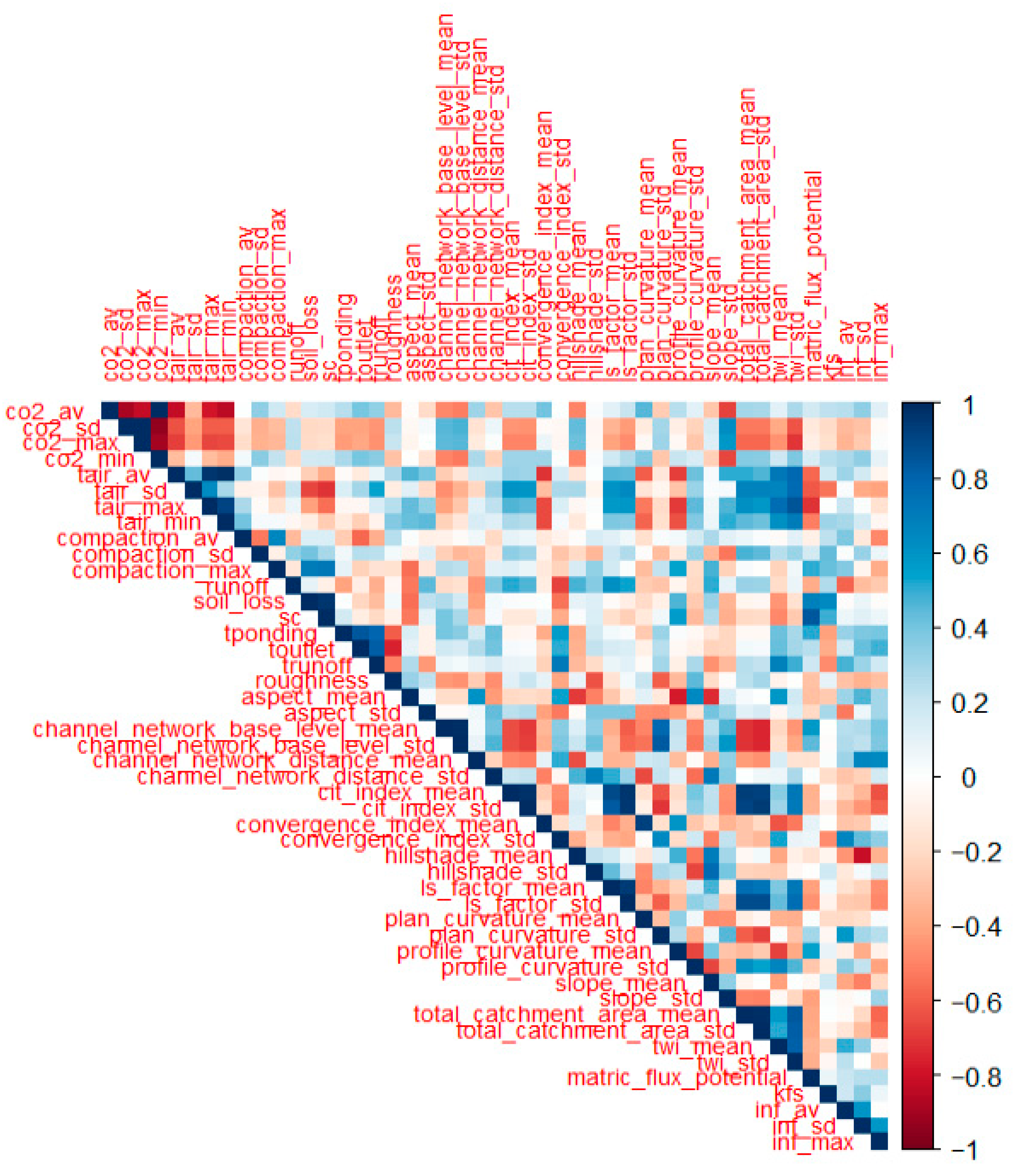
To reduce dimensionality and assess collinearity, Pearson correlation coefficients were calculated [48,49] using the cor() function with pairwise complete observations. A threshold of |r| > 0.7 was used to select explanatory variables relevant to the target variable (e.g., soil_loss, runoff, or sc). The results were visualized with corrplot. Although Pearson correlation was initially used to filter highly collinear variables (|r| > 0.7), the primary objective was not to exclude non-linear associations but to simplify the model due to the low sample size. We recognize that alternative methods like VIF or PCA could also be employed in future work to retain variables with non-linear explanatory power. Scatterplot matrices (pairwise plots) were created to explore linear and non-linear trends using the base R function pairs(). Additionally, simple linear relationships were visualized using ggplot2 with geom_point() and geom_smooth (method = “lm”).

2.3.2. Model Construction

Random Forest models were implemented using the randomForest package in R with 500 trees (ntree = 500). The number of variables randomly sampled at each split (mtry) was set to 1, a conservative choice aimed at reducing the risk of overfitting given the limited dataset (n = 10). We did not constrain tree depth or minimum node size, as the primary objective was to explore variable importance rather than optimize predictive accuracy. Variable importance was assessed using two standard metrics: the percentage increase in mean squared error (%IncMSE) and the increase in node purity (IncNodePurity). To validate model performance, we randomly split the dataset into a training set (80%) and a hold-out test set (20%) using the caret::createDataPartition() function. All training, feature selection, and internal validation (via 5-fold cross-validation) were conducted on the training subset. Model performance was then evaluated on the independent test set using Root Mean Square Error (RMSE). Given the small sample size, results are interpreted heuristically to identify potentially relevant explanatory variables rather than for predictive generalization.
Complementary to Random Forest models, multiple linear regression (MLR) models were fitted using the lm() function in R. Diagnostic plots (e.g., residuals vs. fitted, Q-Q plots, scale-location, and leverage) were used to evaluate model assumptions. Both MLR and RF approaches were applied to the three erosion-related response variables (soil loss, sediment concentration, and runoff), and their performance was compared using R2 and RMSE values.
The methodological workflow implemented in this study is summarized in the following flowchart (Figure 3), which integrates UAV-based data acquisition, field experiments, laboratory analyses, and statistical modeling.

3. Results and Discussion

3.1. Descriptive Statistics of the In-Situ Experiments and Measurements, and UAV-Survey

The analysis of infiltration dynamics using the mini-disc infiltrometer revealed relatively homogeneous surface conditions across the citrus orchard, which coincided with the study conducted by [50] in the conventional citrus plantation. Average infiltration rates, based on ten replicated measurements, ranged from approximately 1.4 to 3.1 mm·min−1, values typical of moderately compacted soils with low to medium permeability [51,52]. The boxplot shows low dispersion and a nearly symmetric distribution, supporting the presence of uniform infiltration patterns. Although a few individual points were recorded above the whiskers, these likely represent minor field-scale variability rather than systemic heterogeneity (Figure 4a).
In contrast, the saturated hydraulic conductivity (Kfs) values, obtained with the Guelph permeameter (Figure 4b), exhibited substantial variability among samples, spanning from <2.0 mm·h−1 to >3.5 mm·h−1. The distribution was strongly skewed by several high outliers, pointing to possible structural differences in the subsoil and heterogeneous pore connectivity, likely influenced by localized macropore flow, coinciding with other crops such as olive orchards and vineyards [53,54]. This variability underscores the complexity of water movement in structured agricultural soils, where preferential pathways can strongly alter infiltration rates [55,56]. Similarly, matric flux potential (MFP) values remained generally stable across the orchard, clustering tightly around 1.59 × 10⁻⁴ cm2·min−1, except for a single elevated observation (Figure 4c). This consistency suggests relatively uniform matric suction and water release potential under unsaturated conditions.
The rainfall simulation experiments provided further insight into the initial hydrological response of the soils. The temporal parameters—Time to Ponding (Tp), Time to Outlet Flow (To), and Time to Runoff (Tr); Figure 4d—captured distinct phases in water movement. Ponding occurred rapidly (3–15 s) and with minimal variability, reflecting limited storage capacity at the surface. In contrast, outlet and runoff initiation times showed greater dispersion (9–22 s and 10–25 s, respectively), suggesting microtopographic differences and variability in flow connectivity across the plots. The narrow ranges observed for these parameters are consistent with the uniform surface texture inferred from infiltration measurements [57,58]. The temporal evolution of runoff (L·m−2), sediment yield (g·m−2), and sediment concentration (g·L−1) revealed a consistent erosive pattern across replicates (Figure 4e). Runoff increased sharply in the first minutes, peaking between 1:00 and 2:30 min, before gradually stabilizing. Sediment yield followed a similar pattern, with maximum detachment and transport during early stages, when soil cohesion was lowest and surface sealing most active. Sediment concentration peaked in the initial interval (0–30 s), consistent with splash erosion dominance, before dilution effects reduced concentrations [36,59]. These findings collectively highlight the effectiveness of the rainfall simulator in reproducing early-stage erosive dynamics [60,61].
In Figure 5, soil respiration and compaction results are depicted in a different heatmaps. CO2 measurements peak in plots 6 and 9, suggesting hotspots of microbial activity likely driven by favorable moisture or organic matter conditions [62,63]. However, the temperature at plot 6 appears anomalously high or incorrectly recorded (gray bar), which warrants further investigation. Soil compaction is highest in the center column, particularly from plots 2 to 10, indicating consistent mechanical pressure likely from repeated machinery traffic [64,65]. Interestingly, despite elevated compaction, high CO2 levels still appear, implying that microbial activity may persist even under physical soil stress, or that surface conditions remain aerated [66]. These observations support the need for integrated monitoring, as respiration hotspots may not always align with assumptions based solely on compaction or temperature.
Finally, the morphometric characterization using SAGA GIS (Table 1) depicts a landscape of gentle relief but marked spatial heterogeneity. While the orchard’s topography was predominantly flat, high-resolution LiDAR enabled the detection of microtopographic features such as mounds, furrows, and subtle drainage paths [16,67]. These features, though minor in gradient, significantly influenced local hydrological behavior. Morphometric indices were derived from the DTM after vegetation filtering using standard ground classification algorithms to eliminate canopy influence. Slopes were generally low (0.1–0.2) and hillshade values consistent (~0.8), yet several indices indicate pronounced contrasts. Channel Network Base Level (1.8–4.5) and Distance (0.1–0.6) varied little, pointing to stable relative incision. By contrast, the Convergence Index (−13.3 to +13.7) and CIT Index (0.0–5.5) emphasize the alternation between convergent hollows and divergent ridges, which directly influences runoff concentration and sediment redistribution. LS Factor (0.6–3.3) and TWI (2.6–6.0) variability further suggest differences in erosion potential and wetness conditions, while Total Catchment Area showed the highest variability (1.4–427.7), reflecting sharp contrasts in upslope contributing area. The combination of these metrics indicates a terrain with alternating convergent–divergent patterns, variable hydrological accumulation, and localized zones more susceptible to erosion and moisture accumulation [68,69,70].

3.2. Correlation Matrix to Define Key Related Hydro-Pedological Variables

Figure 6 shows the Pearson correlation coefficients among all numerical predictors and the target variable (soil loss), allowing visual identification of multicollinearity and key pairwise relationships between measured variables and the target parameters of soil loss and runoff. The results indicated that strong correlations (r > 0.6) were found primarily with soil loss, while no substantial associations were observed with runoff. Maximum soil compaction also exhibited a strong positive correlation (r = 0.71), suggesting that surface consolidation contributes significantly to increased erosion potential [71]. Similarly, matric flux potential (r = 0.69) and saturated hydraulic conductivity (Kfs) (r = 0.65) were positively associated with soil loss, indicating that hydraulic properties play a critical role in modulating infiltration-excess runoff and sediment yield [54]. Interestingly, a negative correlation was found between the standard deviation of air temperature (Tair_SD) and soil loss (r = −0.67), potentially reflecting the influence of temperature variability on soil moisture dynamics and vegetation cover, although this is an idea to be explored in the future. These findings highlight the combined effects of surface conditions, hydraulic behavior, and microclimatic variability on erosion responses in citrus orchards, reinforcing the importance of integrating multi-scale field and terrain data in soil degradation assessments [72,73,74].

3.3. Prediction of Key Hydro-Pedological Variables and Processes

As a starting point for the results related to the modeling approach (Figure 7), we jointly address the three hydrological responses: soil loss, sediment concentration (SC), and runoff.
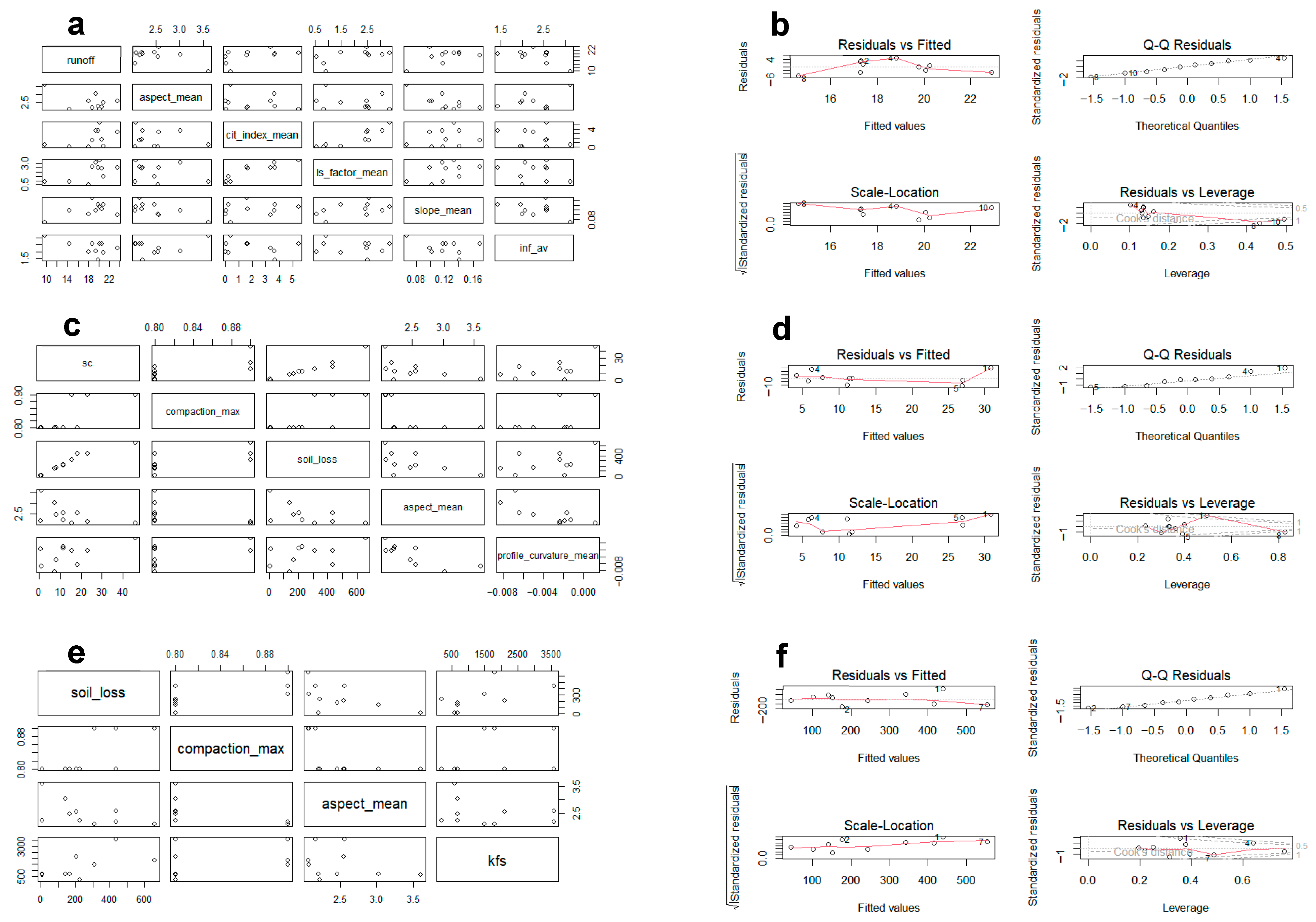
Table 2 summarizes the model performance metrics obtained using the 20% test data. The performance of the soil loss and SC models were moderate (R2 = 0.28–0.29), while the runoff model performed poorly. Moreover, to assess model performance beyond internal fit, we implemented a hold-out validation approach by splitting the dataset into a training set (80%) and a test set (20%), repeated for each target variable (soil loss, runoff, and sediment concentration). In the training phase, Random Forest models achieved moderate to strong fits, with R2 values ranging from 0.68 to 0.75 depending on the variable. However, performance on the test set was noticeably lower (R2 between 0.12 and 0.30), reflecting the expected instability due to the limited sample size (n = 10). Root Mean Square Error (RMSE) values on the test data confirmed this discrepancy, showing increased prediction error relative to the training phase. These results underscore the exploratory nature of our analysis: the machine learning models were not intended to produce robust predictive outputs but to help identify the most influential explanatory variables under the specific conditions of a citrus orchard. The limited generalization is thus an inherent feature of the dataset’s structure and sampling scope.

3.3.1. Runoff

For runoff, a simple linear regression with infiltration average (inf_av) indicates a clear inverse trend: each 1-unit increase in inf_av is associated with a −4.83 unit change in runoff (β = −4.83 ± 2.38), explaining 33.9% of the variance (adjusted R2 = 0.26; F1,8 = 4.10; p = 0.077). The scatterplot shows a steady decline in runoff as infiltration increases, although the 95% CI remains wide, reflecting small sample size. Diagnostic plots reveal centered residuals, mild heteroscedasticity and tail departures, and a few high-leverage points, none exceeding usual Cook’s distance thresholds. Pairwise displays suggest weak or no linear associations of runoff with aspect_mean, cit_index_mean, ls_factor_mean, or slope_mean. A random-forest model performed poorly (% variance explained = −46%, MSE ≈ 20.34), with unstable importance scores—consistent with limited data and weak nonlinear signal. Overall, the evidence supports infiltration capacity as a primary control on runoff, but results should be considered tentative, warranting larger samples and, potentially, transformations or mixed/regularized models.

3.3.2. Sediment Concentration

Exploratory analyses indicate a clear positive association between SC and maximum compaction: SC increases steadily from low values at ~0.80 compaction to markedly higher values near 0.90, although the 95% confidence band is wide, reflecting limited sample size and dispersion. Pairwise plots show weak or no linear relationships between SC and aspect_mean or profile_curvature_mean, and no consistent monotonic pattern with soil_loss. Diagnostic plots for the SC-compaction fit show centered residuals with mild heteroscedasticity and tail departures from normality, plus a few high-leverage observations. Overall, these results suggest that surface compaction is the main proximal control on SC in our dataset, while topographic metrics contribute little; however, inference should be cautious given leverage points and the small n.

3.3.3. Soil Loss

The multiple linear regression model for soil loss (soil_loss) using maximum values of compaction (compaction_max) aspect_mean, and kfs explained 67.8% of the variability (R2), with an adjusted R2 of 0.52 and a global test close to significance (F = 4.22; p = 0.063). Maximum compaction showed the largest positive effect (β = 1.74 × 10³), followed by kfs (β = 0.069), while aspect_mean had a negative effect (β = −89.5); none of these were statistically significant (p > 0.15–0.47). Diagnostic plots indicated centered residuals, slight heteroscedasticity, and tail deviations, with some high-leverage points. The random forest model explained 28.8% of the variance (MSE ≈ 2.67 × 10⁴) and confirmed the relevance of compaction_max and kfs (highest %IncMSE and IncNodePurity), while aspect_mean contributed less information. Overall, the results suggest that compaction and hydraulic conductivity are key factors influencing soil loss; however, the small sample size and observed variability highlight the need for expanding the dataset and exploring transformations or regularization.

3.4. Challenges and Main Weaknesses

One important limitation of this study is the reduced number of spatial sampling points (n = 10), which constrains the generalizability and statistical power of both conventional and machine learning analyses. While each point was thoroughly characterized with repeated field measurements, and averaged to obtain representative values, this aggregation inevitably reduces the ability to model uncertainty within sampling units. Future work should consider hierarchical or mixed-effects modeling frameworks to incorporate both intra-point variance (via more replicates od the rainfall simulations) and spatial heterogeneity (upper, backslope and footslope). Similarly, expanding the number of plot units would allow for more robust machine learning applications and external validation. Nevertheless, the current approach serves as a methodological proof-of-concept for integrating proximal sensing and field experimentation in erosion diagnostics under real-world constraints. We acknowledge that Random Forest is generally robust to multicollinearity and capable of handling a large number of predictors, including the detection of non-linear patterns. Thus, in principle, a preliminary filtering of variables based on Pearson correlation is not strictly necessary. However, in our initial experiments the performance of the models was relatively weak. For this reason, and following recommendations in the literature (e.g., [48,49]), we applied a correlation-based variable reduction (|r| > 0.7) to minimize redundancy and to facilitate model interpretation. This approach was also combined with scatterplot matrices and pairwise plots to examine both linear and non-linear relationships. Nevertheless, we agree that it would be valuable to also test Random Forest without prior filtering in order to verify whether model performance improves when all predictors are retained. In addition, it will be worthy to explore other feature selection strategies embedded within the model, as well as dimensionality reduction through PCA, to compare the outcomes. This would allow us to assess more comprehensively whether the correlation-based filtering might have constrained the predictive capacity of the models. We acknowledge that the aggregation of repeated field measurements into averaged values at each sampling point may have reduced the capacity to model intra-point variability. Future studies should explore hierarchical modeling strategies (e.g., linear mixed-effects models) to integrate replication structure and better represent uncertainty components at multiple scales.
Future studies may consider dimension-reduction methods such as Partial Least Squares (PLS) regression, which are well suited for small sample sizes with high-dimensional predictors and have been extensively applied in environmental and chemometric contexts.
The field experiments conducted in a citrus orchard near Doñana National Park (Seville, southern Spain) revealed crucial insights into erosion processes in flat Mediterranean agroecosystems. Through the integration of UAV-LiDAR–derived topographic variables and detailed field measurements, we found that compaction and infiltration dynamics are the dominant controls on hydrological responses [15,50]. Soil loss was most strongly associated with maximum soil compaction and near-surface saturated hydraulic conductivity (Kfs), with aspect_mean showing a negative relationship—likely reflecting the influence of solar exposure and biological soil cover, particularly moss. Indeed, LiDAR-derived aspect maps showed shaded microsites beneath the citrus canopy (north- and east-facing orientations) with visible moss growth, which appeared to modulate erosion by increasing surface stability (Figure 8a,b). These subtle biophysical differences significantly impacted model outputs [61]. For sediment concentration (SC), surface compaction was the strongest predictor, while topographic variables contributed little explanatory power although they demonstrated the relevance of the sediment mobilisation close to the trees and the compaction in the inter-row areas (Figure 8c; [64,75]). Infiltration emerged as the primary driver for runoff generation, with an inverse relationship between infiltration and runoff clearly established. However, all models were constrained by limited sample size, moderate heteroscedasticity, and the presence of high-leverage observations. Random forest models confirmed the central role of compaction and Kfs but struggled to capture variance in runoff and SC, underscoring the challenge of applying machine learning with small, noisy datasets. Overall, our results highlight the feasibility and value of integrating proximal sensing with field experiments to identify erosion hotspots and optimize monitoring protocols in perennial cropping systems. Yet, future studies should prioritize larger datasets, additional microclimatic and biological indicators which affect aggregate stability (Figure 8a,d), and regularized modeling frameworks to improve predictive reliability.
The relatively weak contribution of UAV-LiDAR to the erosion models in our study is primarily explained by the very gentle relief and limited topographic variability of the citrus orchard as other researchers confirmed [76]. In such flat agroecosystems, morphometric indices derived from high-resolution LiDAR data can provide little differentiation among sampling points, thereby constraining their explanatory capacity. This result should not be interpreted as a limitation of the technology itself but rather as a reflection of the site-specific conditions, which reduce the sensitivity of terrain attributes to capture erosion drivers using visual inspections [77]. Nevertheless, UAV-LiDAR offered important indirect benefits by ensuring centimeter-level georeferencing accuracy, maintaining microtopographic consistency, and providing a replicable framework for future monitoring [78]. These strengths highlight that while UAV-LiDAR may add limited explanatory power in low-relief environments, it remains a valuable tool for scaling up erosion assessments, especially when applied in more heterogeneous landscapes.

4. Conclusions

This study demonstrates that integrating UAV-LiDAR–derived morphometric variables with standardized field experiments provides valuable insights into the drivers of soil erosion in citrus orchards under Mediterranean conditions. Despite the limited sample size, considering the difficulties to perform such number of parallel experiments with four different devices at the same time during summer (dry soils) with enough trained researchers, consistent physical controls emerged across multiple models: soil loss was primarily influenced by maximum soil compaction and saturated hydraulic conductivity (Kfs); sediment concentration was associated with surface compaction; and runoff was inversely related to average infiltration. The aspect orientation derived from LiDAR data revealed the presence of moss and more stable surface conditions in shaded areas under the citrus canopy, emphasizing the role of microclimatic and biological factors in erosion dynamics. Although machine learning approaches such as random forests were useful in identifying relevant predictors, their performance was constrained by data variability and sample limitations. Overall, this framework highlights a cost-effective and scalable strategy for monitoring erosion risk, prioritizing key variables, and guiding sustainable land management in perennial cropping systems.

Supplementary Materials

The following supporting information can be downloaded at: https://www.mdpi.com/article/10.3390/w17243541/s1.

Author Contributions

J.R.-C.: Conceptualization, Methodology, Formal Analysis, Data Collection, Investigation, Resources, Writing—Original Draft, Writing—Review & Editing, Visualization, Supervision; L.C.-R.: Data Collection, Laboratory work, Writing—Original Draft; L.M.-C.: Data Collection, Laboratory work, Writing—Original Draft; J.G.-V.: Data Collection, Writing—Original Draft; M.T.G.-M.: Data Collection, Writing—Original Draft; V.R.-G.: Conceptualization, Methodology, Data Collection, Investigation, Resources, Writing—Review & Editing, Supervision, and Project Administration. All authors have read and agreed to the published version of the manuscript.

Funding

This research was carried out within the framework of the projects: (i) “Monitorización hiper-espectral para el manejo de los cítricos en el contexto del cambio climático (CITRUSMART)”, Junta de Andalucía (GOPG-SE-23-0024, 2023–2025); (ii) “Desarrollo de productos basados en los nuevos sensores satelitales hiperespectrales europeos e IA para la caracterización de estresores en tierras de cultivo (HIPROESTRES)” (grant number PID2023-152656OB-I00), within the Programa Estatal de Investigación Científica, Técnica y de Innovación (2021–2023) funded by the Ministerio de Ciencia, Innovación y Universidades.

Data Availability Statement

The original contributions presented in this study are included in the article. Further inquiries can be directed to the corresponding author.

Acknowledgments

During the preparation of this work the authors used Chat GPT in order to review the Flow and grammar of the text. After using this tool/service, the authors reviewed and edited the content as needed and take full responsibility for the content of the published article.

Conflicts of Interest

The authors declare no conflicts of interest.

References

  1. Seeger, M. (Ed.) Understanding and Preventing Soil Erosion; Burleigh Dodds Science Publishing: London, UK, 2024; ISBN 978-1-003-58788-0. [Google Scholar]
  2. Chen, Y.; De Geeter, S.; Poesen, J.; Matthews, F.; Campforts, B.; Borrelli, P.; Panagos, P.; Vanmaercke, M. Global Patterns of Gully Occurrence and Their Sensitivity to Environmental Changes. Int. Soil Water Conserv. Res. 2025. [Google Scholar] [CrossRef]
  3. Visser, S.; Keesstra, S.; Maas, G.; de Cleen, M.; Molenaar, C. Soil as a Basis to Create Enabling Conditions for Transitions Towards Sustainable Land Management as a Key to Achieve the SDGs by 2030. Sustainability 2019, 11, 6792. [Google Scholar] [CrossRef]
  4. Sanaullah, M.; Usman, M.; Wakeel, A.; Cheema, S.A.; Ashraf, I.; Farooq, M. Terrestrial Ecosystem Functioning Affected by Agricultural Management Systems: A Review. Soil Tillage Res. 2020, 196, 104464. [Google Scholar] [CrossRef]
  5. Alliaume, F.; Rossing, W.A.H.; Tittonell, P.; Jorge, G.; Dogliotti, S. Reduced Tillage and Cover Crops Improve Water Capture and Reduce Erosion of Fine Textured Soils in Raised Bed Tomato Systems. Agric. Ecosyst. Environ. 2014, 183, 127–137. [Google Scholar] [CrossRef]
  6. Casalí, J.; Gastesi, R.; Álvarez-Mozos, J.; De Santisteban, L.M.; de Lersundi, J.D.V.; Giménez, R.; Larrañaga, A.; Goñi, M.; Agirre, U.; Campo, M.A.; et al. Runoff, Erosion, and Water Quality of Agricultural Watersheds in Central Navarre (Spain). Agric. Water Manag. 2008, 95, 1111–1128. [Google Scholar] [CrossRef]
  7. Fu, B.; Merritt, W.S.; Croke, B.F.W.; Weber, T.R.; Jakeman, A.J. A Review of Catchment-Scale Water Quality and Erosion Models and a Synthesis of Future Prospects. Environ. Model. Softw. 2019, 114, 75–97. [Google Scholar] [CrossRef]
  8. Keesstra, S.; Nunes, J.; Novara, A.; Finger, D.; Avelar, D.; Kalantari, Z.; Cerdà, A. The Superior Effect of Nature Based Solutions in Land Management for Enhancing Ecosystem Services. Sci. Total Environ. 2018, 610–611, 997–1009. [Google Scholar] [CrossRef]
  9. Albaladejo, J.; Díaz-Pereira, E.; de Vente, J. Eco-Holistic Soil Conservation to Support Land Degradation Neutrality and the Sustainable Development Goals. Catena 2021, 196, 104823. [Google Scholar] [CrossRef]
  10. Cerdan, O.; Govers, G.; Le Bissonnais, Y.; Van Oost, K.; Poesen, J.; Saby, N.; Gobin, A.; Vacca, A.; Quinton, J.; Auerswald, K.; et al. Rates and Spatial Variations of Soil Erosion in Europe: A Study Based on Erosion Plot Data. Geomorphology 2010, 122, 167–177. [Google Scholar] [CrossRef]
  11. García-Ruiz, J.M.; Beguería, S.; Nadal-Romero, E.; González-Hidalgo, J.C.; Lana-Renault, N.; Sanjuán, Y. A Meta-Analysis of Soil Erosion Rates across the World. Geomorphology 2015, 239, 160–173. [Google Scholar] [CrossRef]
  12. Panagos, P.; Borrelli, P.; Meusburger, K.; Alewell, C.; Lugato, E.; Montanarella, L. Estimating the Soil Erosion Cover-Management Factor at the European Scale. Land Use Policy 2015, 48, 38–50. [Google Scholar] [CrossRef]
  13. Cerdà, A.; Rodrigo-Comino, J.; Giménez-Morera, A.; Novara, A.; Pulido, M.; Kapović-Solomun, M.; Keesstra, S.D. Policies Can Help to Apply Successful Strategies to Control Soil and Water Losses. The Case of Chipped Pruned Branches (CPB) in Mediterranean Citrus Plantations. Land Use Policy 2018, 75, 734–745. [Google Scholar] [CrossRef]
  14. Duan, J.; Liu, Y.-J.; Yang, J.; Tang, C.-J.; Shi, Z.-H. Role of Groundcover Management in Controlling Soil Erosion under Extreme Rainfall in Citrus Orchards of Southern China. J. Hydrol. 2020, 582, 124290. [Google Scholar] [CrossRef]
  15. Jianjun, W.; Quansheng, L.; Lijiao, Y. Effect of intercropping on soil erosion in young citrus plantation—A simulation study. Chin. J. Appl. Ecol. 2017, 8, 143–146. [Google Scholar]
  16. Bayat, F.; Monfared, A.B.; Jahansooz, M.R.; Esparza, E.T.; Keshavarzi, A.; Morera, A.G.; Fernández, M.P.; Cerdà, A. Analyzing Long-Term Soil Erosion in a Ridge-Shaped Persimmon Plantation in Eastern Spain by Means of ISUM Measurements. Catena 2019, 183, 104176. [Google Scholar] [CrossRef]
  17. Anache, J.A.A.; Wendland, E.C.; Oliveira, P.T.S.; Flanagan, D.C.; Nearing, M.A. Runoff and Soil Erosion Plot-Scale Studies under Natural Rainfall: A Meta-Analysis of the Brazilian Experience. Catena 2017, 152, 29–39. [Google Scholar] [CrossRef]
  18. Bernoux, M.; Cerri, C.C.; Cerri, C.E.P.; Neto, M.S.; Metay, A.; Perrin, A.-S.; Scopel, E.; Tantely, R.; Blavet, D.; de Piccolo, M.C.; et al. Cropping Systems, Carbon Sequestration and Erosion in Brazil: A Review. In Sustainable Agriculture; Lichtfouse, E., Navarrete, M., Debaeke, P., Véronique, S., Alberola, C., Eds.; Springer: Dordrecht, The Netherlands, 2009; pp. 75–85. ISBN 978-90-481-2665-1. [Google Scholar]
  19. Di Prima, S.; Bagarello, V.; Lassabatere, L.; Angulo-Jaramillo, R.; Bautista, I.; Burguet, M.; Cerdà, A.; Iovino, M.; Prosdocimi, M. Comparing Beerkan Infiltration Tests with Rainfall Simulation Experiments for Hydraulic Characterization of a Sandy-Loam Soil. Hydrol. Process. 2017, 31, 3520–3532. [Google Scholar] [CrossRef]
  20. Iserloh, T.; Ries, J.B.; Arnáez, J.; Boix-Fayos, C.; Butzen, V.; Cerdà, A.; Echeverría, M.T.; Fernández-Gálvez, J.; Fister, W.; Geißler, C.; et al. European Small Portable Rainfall Simulators: A Comparison of Rainfall Characteristics. Catena 2013, 110, 100–112. [Google Scholar] [CrossRef]
  21. Vishwakarma, D.K.; Yadav, D.; Kumar, R.; Kumar, R.; Bhat, S.A.; Mirzania, E.; Kuriqi, A. Assessing the Performance of Various Infiltration Models to Improve Water Management Practices. Paddy Water Environ. 2025, 23, 77–93. [Google Scholar] [CrossRef]
  22. Bogunovic, I.; Telak, L.J.; Pereira, P. Experimental Comparison of Runoff Generation and Initial Soil Erosion Between Vineyards and Croplands of Eastern Croatia: A Case Study. Air Soil Water Res. 2020, 13, 1178622120928323. [Google Scholar] [CrossRef]
  23. Telak, L.J.; Dugan, I.; Bogunovic, I. Soil Management and Slope Impacts on Soil Properties, Hydrological Response, and Erosion in Hazelnut Orchard. Soil Syst. 2021, 5, 5. [Google Scholar] [CrossRef]
  24. Fini, A.; Frangi, P.; Mori, J.; Donzelli, D.; Ferrini, F. Nature Based Solutions to Mitigate Soil Sealing in Urban Areas: Results from a 4-Year Study Comparing Permeable, Porous, and Impermeable Pavements. Environ. Res. 2017, 156, 443–454. [Google Scholar] [CrossRef]
  25. Khan, M.O.; Keesstra, S.D.; Słowik-Opoka, E.; Klamerus-Iwan, A.; Liaqat, W. Determining the Role of Urban Greenery in Soil Hydrology: A Bibliometric Analysis of Nature-Based Solutions in Urban Ecosystem. Water 2025, 17, 322. [Google Scholar] [CrossRef]
  26. Gayen, A.; Pourghasemi, H.R.; Saha, S.; Keesstra, S.; Bai, S. Gully Erosion Susceptibility Assessment and Management of Hazard-Prone Areas in India Using Different Machine Learning Algorithms. Sci. Total Environ. 2019, 668, 124–138. [Google Scholar] [CrossRef]
  27. Alexiou, S.; Efthimiou, N.; Karamesouti, M.; Papanikolaou, I.; Psomiadis, E.; Charizopoulos, N. Measuring Annual Sedimentation through High Accuracy UAV-Photogrammetry Data and Comparison with RUSLE and PESERA Erosion Models. Remote Sens. 2023, 15, 1339. [Google Scholar] [CrossRef]
  28. Gómez Gutiérrez, Á.; Schnabel, S.; Lavado Contador, F.; De Sanjosé, J.J.; Atkinson Gordo, A.; Pulido Fernández, M.; Sánchez Fernández, M. Studying the Influence of Livestock Pressure on Gully Erosion in Rangelands of SW Spain by Means of the Uav+sfm Workflow. Boletín Asoc. Geógrafos Españoles 2018, 78, 66–88. [Google Scholar] [CrossRef]
  29. IUSS-WRB. World Reference Base for Soil Resources. International Soil Classification System for Naming Soils and Creating Legends for Soil Maps, 4th ed.; International Union of Soil Sciences (IUSS): Vienna, Austria, 2022. [Google Scholar]
  30. Crema, S.; Cavalli, M. SedInConnect: A Stand-Alone, Free and Open Source Tool for the Assessment of Sediment Connectivity. Comput. Geosci. 2018, 111, 39–45. [Google Scholar] [CrossRef]
  31. Ries, J.B.; Iserloh, T.; Seeger, M.; Gabriels, D. Rainfall Simulations—Constraints, Needs and Challenges for a Future Use in Soil Erosion Research. Z. Geomorphol. 2013, 57, 1–10. [Google Scholar] [CrossRef]
  32. Carollo, F.G.; Caruso, R.; Ferro, V.; Serio, M.A. Characterizing the Kamphorst Rainfall Simulator for Soil Erosion Investigations. J. Hydrol. 2024, 643, 132025. [Google Scholar] [CrossRef]
  33. Hlavčová, K.; Danáčová, M.; Kohnová, S.; Szolgay, J.; Valent, P.; Výleta, R. Estimating the Effectiveness of Crop Management on Reducing Flood Risk and Sediment Transport on Hilly Agricultural Land—A Myjava Case Study, Slovakia. Catena 2019, 172, 678–690. [Google Scholar] [CrossRef]
  34. Iserloh, T.; Fister, W.; Seeger, M.; Willger, H.; Ries, J.B. A Small Portable Rainfall Simulator for Reproducible Experiments on Soil Erosion. Soil Tillage Res. 2012, 124, 131–137. [Google Scholar] [CrossRef]
  35. Cerdà, A. The Influence of Aspect and Vegetation on Seasonal Changes in Erosion under Rainfall Simulation on a Clay Soil in Spain. Can. J. Soil Sci. 1998, 78, 321–330. [Google Scholar] [CrossRef]
  36. Cerdà, A.; Jurgensen, M.F. Ant Mounds as a Source of Sediment on Citrus Orchard Plantations in Eastern Spain. A Three-Scale Rainfall Simulation Approach. Catena 2011, 85, 231–236. [Google Scholar] [CrossRef]
  37. Saleh, A. Soil Roughness Measurement: Chain Method. J. Soil Water Conserv. 1993, 48, 527–529. [Google Scholar] [CrossRef]
  38. Ortega, J.P.; Cambronero, L.; Alcarria Salas, M.; Rodríguez, J.L.; Durán-Zuazo, V.H.; Keesstra, S.D.; Rodrigo-Comino, J. Conducting an in Situ Evaluation of Erodibility in a Mediterranean Semi-Arid and Conventional Vineyard in Granada Province (Southern Spain) through Rainfall Simulation Experiments. Euro-Mediterr. J. Environ. Integr. 2024, 9, 797–808. [Google Scholar] [CrossRef]
  39. Rodrigo-Comino, J.; Bogunovic, I.; Mohajerani, H.; Pereira, P.; Cerdà, A.; Ruiz-Sinoga, J.; Ries, J. The Impact of Vineyard Abandonment on Soil Properties and Hydrological Processes. Vadose Zone J. 2017, 16, 1–7. [Google Scholar] [CrossRef]
  40. Jobbágy, J.; Krištof, K.; Angelovič, M.; Zsembeli, J. Evaluation of Soil Infiltration Variability in Compacted and Uncompacted Soil Using Two Devices. Water 2023, 15, 1918. [Google Scholar] [CrossRef]
  41. Naik, A.P.; Pekkat, S. Time Dependence of Hydraulic Parameters Estimation from Transient Analysis of Mini Disc Infiltrometer Measurements. Eur. J. Soil Sci. 2022, 73, e13228. [Google Scholar] [CrossRef]
  42. Reynolds, W.D. The Guelph Permeameter Method for in Situ Measurement of Field-Saturated Hydraulic Conductivity and Matric Flux Potential. Ph.D. Thesis, University of Guelph, Guelph, ON, Canada, 1986. [Google Scholar]
  43. Arredondo, A.M.; Mirzaei, M.; Wu, G.-L.; Keshavarzi, A.; Durán-Zuazo, V.H.; Bernardo, F.S.; Rodrigo-Comino, J. Evaluating Soil Respiration and Water Infiltration in Esparto Grasslands: The Effects of Hillslope Position and Soil Management in Arid, Human-Affected Mediterranean Environments. Discov. Sustain. 2025, 6, 421. [Google Scholar] [CrossRef]
  44. Madalina, V.; Valentina, C.; Natalia, E.; Lucian, L.; Monica, M.; Anda, R.; Norbert, B.; Madalina, B.; Silvius, S.; György, D. Experimental Determination of Carbon Dioxide Flux in Soil and Correlation with Dependent Parameters. IOP Conf. Ser. Earth Environ. Sci. 2020, 616, 012010. [Google Scholar] [CrossRef]
  45. Keller, T.; Colombi, T.; Ruiz, S.; Schymanski, S.J.; Weisskopf, P.; Koestel, J.; Sommer, M.; Stadelmann, V.; Breitenstein, D.; Kirchgessner, N.; et al. Soil Structure Recovery Following Compaction: Short-Term Evolution of Soil Physical Properties in a Loamy Soil. Soil Sci. Soc. Am. J. 2021, 85, 1002–1020. [Google Scholar] [CrossRef]
  46. Khemis, C.; Abrougui, K.; Mohammadi, A.; Gabsi, K.; Dorbolo, S.; Mercatoris, B.; Mutuku, E.; Cornelis, W.; Chehaibi, S. Development of Artificial Neural Networks to Predict the Effect of Tractor Speed on Soil Compaction Using Penetrologger Test Results. Processes 2022, 10, 1109. [Google Scholar] [CrossRef]
  47. Pulido, M.; Schnabel, S.; Lavado Contador, J.F.; Lozano-Parra, J.; Gómez-Gutiérrez, Á.; Brevik, E.C.; Cerdà, A. Reduction of the Frequency of Herbaceous Roots as an Effect of Soil Compaction Induced by Heavy Grazing in Rangelands of SW Spain. Catena 2017, 158, 381–389. [Google Scholar] [CrossRef]
  48. Dormann, C.F.; Elith, J.; Bacher, S.; Buchmann, C.; Carl, G.; Carré, G.; Marquéz, J.R.G.; Gruber, B.; Lafourcade, B.; Leitão, P.J.; et al. Collinearity: A Review of Methods to Deal with It and a Simulation Study Evaluating Their Performance. Ecography 2013, 36, 27–46. [Google Scholar] [CrossRef]
  49. Kyriazos, T.; Poga, M. Dealing with Multicollinearity in Factor Analysis: The Problem, Detections, and Solutions. Open J. Stat. 2023, 13, 404–424. [Google Scholar] [CrossRef]
  50. Di Prima, S.; Rodrigo-Comino, J.; Novara, A.; Iovino, M.; Pirastru, M.; Keesstra, S.D.; Cerdà, A. Soil Physical Quality of Citrus Orchards Under Tillage, Herbicide, and Organic Managements. Pedosphere 2018, 28, 463–477. [Google Scholar] [CrossRef]
  51. Basche, A.D.; DeLonge, M.S. Comparing Infiltration Rates in Soils Managed with Conventional and Alternative Farming Methods: A Meta-Analysis. PLoS ONE 2019, 14, e0215702. [Google Scholar] [CrossRef] [PubMed]
  52. Jagdale, S.; Nimbalkar, P. Infiltration Studies of Different Soils under Different Soil Conditions and Comparison of Infiltration Models with Field Data. Int. J. Eng. Technol. Sci. 2012, 3, 154–157. [Google Scholar]
  53. Rodrigo-Comino, J.; Taguas, E.; Seeger, M.; Ries, J.B. Quantification of Soil and Water Losses in an Extensive Olive Orchard Catchment in Southern Spain. J. Hydrol. 2018, 556, 749–758. [Google Scholar] [CrossRef]
  54. Rodrigo-Comino, J.; Ruiz Sinoga, J.D.; Senciales González, J.M.; Guerra-Merchán, A.; Seeger, M.; Ries, J.B. High Variability of Soil Erosion and Hydrological Processes in Mediterranean Hillslope Vineyards (Montes de Málaga, Spain). Catena 2016, 145, 274–284. [Google Scholar] [CrossRef]
  55. Amini, M.; Rasoulzadeh, A.; Mobaser, J.A.; Ahmadabad, Y.H.; Pollacco, J.A.P.; Fernández-Gálvez, J. Hydro-Pedotransfer Functions to Estimate Evaporation from Bare Soil Surface in Semi-Arid Regions. Air Soil Water Res. 2025, 18, 11786221251349047. [Google Scholar] [CrossRef]
  56. Angulo-Jaramillo, R.; Bagarello, V.; Iovino, M.; Lassabatere, L. Infiltration Measurements for Soil Hydraulic Characterization; Springer: Cham, Switzerland, 2016; ISBN 978-3-319-31788-5. [Google Scholar]
  57. Cerdà, A.; González-Pelayo, Ó.; Giménez-Morera, A.; Jordán, A.; Pereira, P.; Novara, A.; Brevik, E.C.; Prosdocimi, M.; Mahmoodabadi, M.; Keesstra, S. Use of Barley Straw Residues to Avoid High Erosion and Runoff Rates on Persimmon Plantations in Eastern Spain under Low Frequency–High Magnitude Simulated Rainfall Events. Soil Res. 2016, 54, 154–165. [Google Scholar] [CrossRef]
  58. Keesstra, S.; Pereira, P.; Novara, A.; Brevik, E.C.; Azorin-Molina, C.; Parras-Alcántara, L.; Jordán, A.; Cerdà, A. Effects of Soil Management Techniques on Soil Water Erosion in Apricot Orchards. Sci. Total Environ. 2016, 551–552, 357–366. [Google Scholar] [CrossRef]
  59. Cerdà, A.; Ackermann, O.; Terol, E.; Rodrigo-Comino, J. Impact of Farmland Abandonment on Water Resources and Soil Conservation in Citrus Plantations in Eastern Spain. Water 2019, 11, 824. [Google Scholar] [CrossRef]
  60. de Lima, J.L.M.P.; Carvalho, S.C.P.; de Lima, M.I.P. Rainfall Simulator Experiments on the Importance o of When Rainfall Burst Occurs during Storm Events on Runoff and Soil Loss. Z. Geomorphol. 2013, 57, 91–109. [Google Scholar] [CrossRef]
  61. Seeger, M. Uncertainty of Factors Determining Runoff and Erosion Processes as Quantified by Rainfall Simulations. Catena 2007, 71, 56–67. [Google Scholar] [CrossRef]
  62. Fiener, P.; Dlugoß, V.; Korres, W.; Schneider, K. Spatial Variability of Soil Respiration in a Small Agricultural Watershed—Are Patterns of Soil Redistribution Important? Catena 2012, 94, 3–16. [Google Scholar] [CrossRef]
  63. Parkin, T.B.; Doran, J.W. Field and Laboratory Tests of Soil Respiration. In Methods for Assessing Soil Quality; Doran, J.W., Jones, A.J., Eds.; Soil Science Society of America Incorporated: Madison, WI, USA, 1996; Volume SSSA Special Publication 49, pp. 231–246. [Google Scholar]
  64. Bogunović, I.; Kisić, I.; Maletić, E.; Perčin, A.; Matošić, S.; Roškar, L. Soil Compaction in Vineyards of Different Ages in Pannonian Croatia. Part I. Influence of Machinery Traffic and Soil Management on Compaction of Individual Horizons. J. Cent. Eur. Agric. 2016, 17, 533–544. [Google Scholar] [CrossRef]
  65. Duttmann, R.; Schwanebeck, M.; Nolde, M.; Horn, R. Predicting Soil Compaction Risks Related to Field Traffic during Silage Maize Harvest. Soil Sci. Soc. Am. J. 2014, 78, 408–421. [Google Scholar] [CrossRef]
  66. Cleveland, C.C.; Nemergut, D.R.; Schmidt, S.K.; Townsend, A.R. Increases in Soil Respiration Following Labile Carbon Additions Linked to Rapid Shifts in Soil Microbial Community Composition. Biogeochemistry 2007, 82, 229–240. [Google Scholar] [CrossRef]
  67. Moradi, E.; Rodrigo-Comino, J.; Terol, E.; Mora-Navarro, G.; Marco da Silva, A.; N. Daliakopoulos, I.; Khosravi, H.; Pulido Fernández, M.; Cerdà, A. Quantifying Soil Compaction in Persimmon Orchards Using ISUM (Improved Stock Unearthing Method) and Core Sampling Methods. Agriculture 2020, 10, 266. [Google Scholar] [CrossRef]
  68. Arabameri, A.; Cerda, A.; Pradhan, B.; Tiefenbacher, J.P.; Lombardo, L.; Bui, D.T. A Methodological Comparison of Head-Cut Based Gully Erosion Susceptibility Models: Combined Use of Statistical and Artificial Intelligence. Geomorphology 2020, 359, 107136. [Google Scholar] [CrossRef]
  69. Keshavarzi, A.; Omran, E.-S.E.; Bateni, S.M.; Pradhan, B.; Vasu, D.; Bagherzadeh, A. Modeling of Available Soil Phosphorus (ASP) Using Multi-Objective Group Method of Data Handling. Model. Earth Syst. Environ. 2016, 2, 157. [Google Scholar] [CrossRef]
  70. Vermeulen, D.; Van Niekerk, A. Machine Learning Performance for Predicting Soil Salinity Using Different Combinations of Geomorphometric Covariates. Geoderma 2017, 299, 1–12. [Google Scholar] [CrossRef]
  71. Capello, G.; Biddoccu, M.; Ferraris, S.; Cavallo, E. Effects of Tractor Passes on Hydrological and Soil Erosion Processes in Tilled and Grassed Vineyards. Water 2019, 11, 2118. [Google Scholar] [CrossRef]
  72. Esteves, M.; Lapetite, J.M. A Multi-Scale Approach of Runoff Generation in a Sahelian Gully Catchment: A Case Study in Niger. Catena 2003, 50, 255–271. [Google Scholar] [CrossRef]
  73. Martínez-Carreras, N.; Krein, A.; Gallart, F.; Iffly, J.F.; Pfister, L.; Hoffmann, L.; Owens, P.N. Assessment of Different Colour Parameters for Discriminating Potential Suspended Sediment Sources and Provenance: A Multi-Scale Study in Luxembourg. Geomorphology 2010, 118, 118–129. [Google Scholar] [CrossRef]
  74. Nunes, J.P.; Seixas, J.; Keizer, J.J. Modeling the Response of Within-Storm Runoff and Erosion Dynamics to Climate Change in Two Mediterranean Watersheds: A Multi-Model, Multi-Scale Approach to Scenario Design and Analysis. Catena 2013, 102, 27–39. [Google Scholar] [CrossRef]
  75. Alameda, D.; Villar, R.; Iriondo, J.M. Spatial Pattern of Soil Compaction: Trees’ Footprint on Soil Physical Properties. For. Ecol. Manag. 2012, 283, 128–137. [Google Scholar] [CrossRef]
  76. Niu, Y.H.; Wang, L.; Wan, X.G.; Peng, Q.Z.; Huang, Q.; Shi, Z.H. A Systematic Review of Soil Erosion in Citrus Orchards Worldwide. Catena 2021, 206, 105558. [Google Scholar] [CrossRef]
  77. Đomlija, P.; Bernat Gazibara, S.; Arbanas, Ž.; Mihalić Arbanas, S. Identification and Mapping of Soil Erosion Processes Using the Visual Interpretation of LiDAR Imagery. ISPRS Int. J. Geo-Inf. 2019, 8, 438. [Google Scholar] [CrossRef]
  78. Donmez, C.; Villi, O.; Berberoglu, S.; Cilek, A. Computer Vision-Based Citrus Tree Detection in a Cultivated Environment Using UAV Imagery. Comput. Electron. Agric. 2021, 187, 106273. [Google Scholar] [CrossRef]
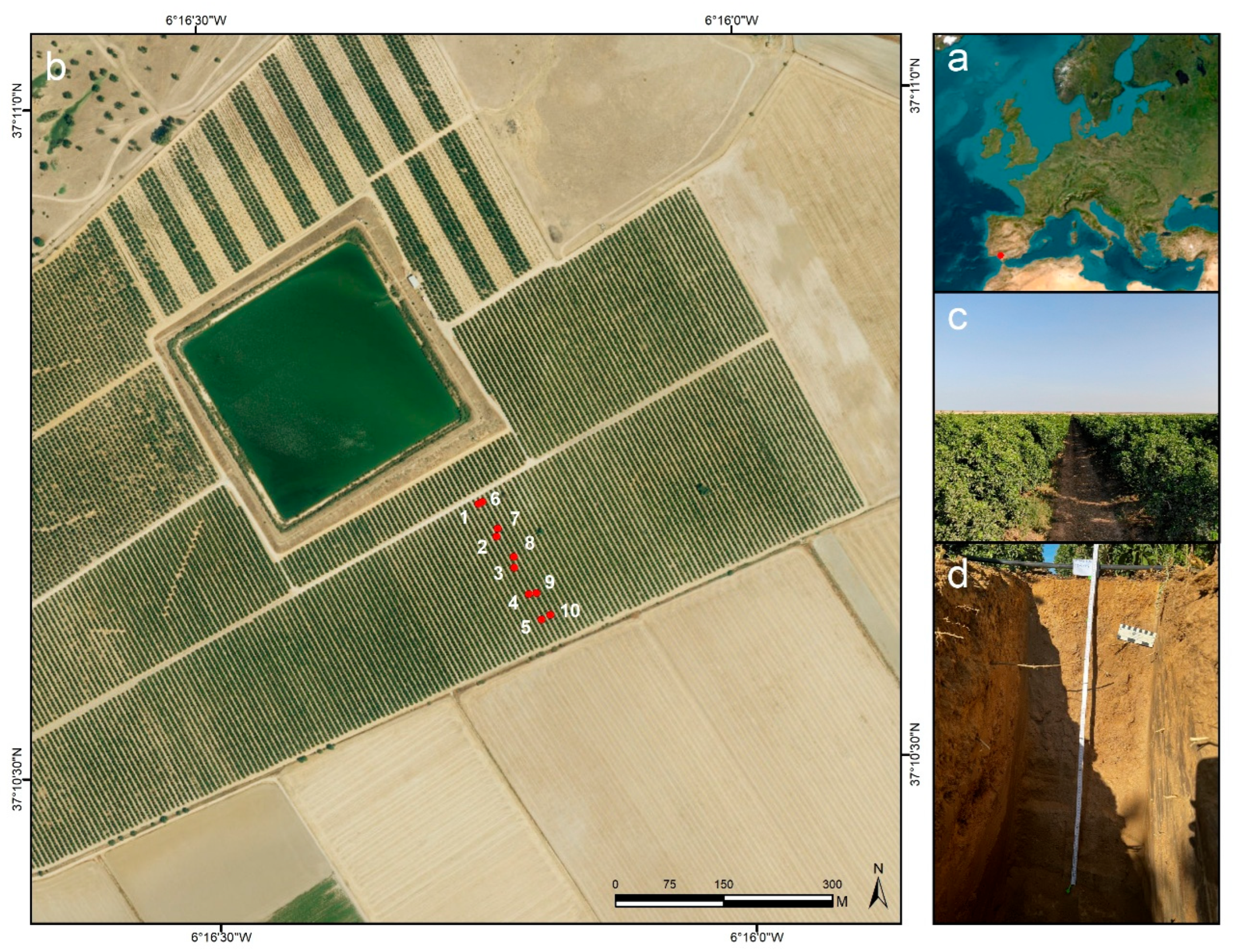
Figure 1. Study area. (a): localization in Europe of the study site; (b): exact localization of the sampled points (1–10) in the citrus orchard plantation; (c): general overview using a UAV; (d): soil profile in the study area (Gleyic regosol; clayic, arenic; IUSS-WRB, 2022 [29]).
Water 17 03541 g001
Figure 2. Methods employed in the field experiments and measurements. (a): Rainfall simulations; (b): Infiltration (mini-disc); (c): Guelph permeameter; (d): Soil compaction; (e): CO2 analysis; (f): soil profile description.
Water 17 03541 g002
Figure 3. Methodological workflow followed in this study [29].
Water 17 03541 g003
Figure 4. Hydrological response of the experiments and measurements. (a): average soil infiltration rates (mini-disc infiltrometer); (b): average soil saturated hydraulic conductivity (Guelph permeameter); (c): average soil flux matric potential; (d): Toutlet (time to outlet), Tponding (time to ponding) and Trunoff (time to runoff generation); (e): runoff, sediment concentration and soil loss per interval using a rainfall simulator.
Water 17 03541 g004
Figure 5. Gas analysis and air temperature, and soil compaction. av: average; max: maximum; min: minimum; sd: standard deviation.
Water 17 03541 g005
Figure 6. Correlation matrix using Pearson linear relationships. av: average; max: maximum; min: minimum; sd: standard deviation; co2: gas analysis of CO2; tair: air temperature; sc: sediment concentration; Toutlet (time to outlet), Tponding (time to ponding) and Trunoff (time to runoff generation); cit_index: connectivity index; TWI: Topographic Wetness Index; ls_factor: LS factor (USLE); kfs: soil saturated hydraulic conductivity.
Water 17 03541 g006
Figure 7. Pairwise scatterplot matrix of runoff, soil loss, and key terrain variables. Each subplot shows the relationship between two variables with fitted trendlines and dispersion patterns. Values are standardized. This matrix helps assess multicollinearity and co-variability between predictors and erosion responses. Pairwise (a,c,e) and residual (b,d,f) graphs show the main results obtained after applying the random forest machine learning technique.
Water 17 03541 g007
Figure 8. Some key factors affecting soil erosion in citrus orchards detected after finishing the study without possible measurements. (a). Biocrusts and catch crops; (b). inter-row areas with bare soils; (c). concave micro-topography where runoff activates soil erosion; (d). example of compacted soil aggregate.
Water 17 03541 g008
Table 1. Basic morphometric statistics derived from LiDAR-based terrain analysis in SAGA GIS. Values correspond to the mean and standard deviation of a 3 × 3 pixel window centered on each sampling point. The indices include: (a) CNBL—Channel Network Base Level (m); (b) CND—Channel Network Distance (m); (c) Convergence Index (unitless); (d) Catchment Area (m2); and (e) TWI—Topographic Wetness Index (unitless, log-transformed ratio of upslope area and slope).
AspectCNBLCNDCIT IndexConv. IndexHillshadeLSFactor Plan Curv.Prof. Curv.SlopeCatch. AreaTWI (Mean)
2.1 ± 1.44.50.3 ± 0.10.1 ± 0−2.6 ± 14.60.80.8 ± 0.40.00.00.16.6 ± 5.93.4 ± 1.5
2.2 ± 1.33.40.5 ± 0.11.7 ± 2.3−3.3 ± 22.30.82.4 ± 2.20.00.00.1129.8 ± 156.64.8 ± 2.6
3.0 ± 2.02.60.6 ± 0.13.6 ± 6.7−13.3 ± 12.70.83.1 ± 3.90.00.00.1246.7 ± 345.15.0 ± 2.8
2.6 ± 1.82.20.3 ± 0.13.4 ± 5.9−8.3 ± 6.60.82.5 ± 3.00.00.00.1344.5 ± 483.95.0 ± 3.0
2.1 ± 1.31.90.1 ± 0.15.5 ± 9.9−6.1 ± 8.60.83.3 ± 4.10.00.00.1427.7 ± 601.94.7 ± 3.2
2.5 ± 1.74.40.3 ± 0.10.2 ± 0.2−11.7 ± 13.70.81.5 ± 1.00.00.00.18.4 ± 6.93.8 ± 1.5
2.2 ± 1.83.40.5 ± 0.11.6 ± 2.7−9.6 ± 10.10.82.6 ± 2.20.00.00.2108.5 ± 150.74.0 ± 2.8
3.6±2.70.6 ± 0.10.4 ± 1.0−7.4 ± 27.70.80.9 ± 1.10.00.00.1183.6 ± 260.66.0 ± 3.1
2.6±2.10.6 ± 00.0 ± 013.7 ± 9.00.80.6 ± 0.50.00.00.11.4 ± 0.32.6 ± 0.8
2.2±1.80.2 ± 0.13.7 ± 9.11.8 ± 7.60.82.5 ± 3.50.00.00.1290.5 ± 539.64.0 ± 3.0
Table 2. Summary of the prediction performance for each model (including RMSE and correlation coefficients between predicted and observed values in the test folds).
ModelDatasetR2RMSEMAENotes
RF (soil_loss)Test (20%)0.29141.9113.6Train/test split, ntree = 500
RF (SC)Test (20%)0.28124.295.4Low signal, short range
RF (Runoff)Test (20%)−0.46NaNNaNPoor model fit
Disclaimer/Publisher’s Note: The statements, opinions and data contained in all publications are solely those of the individual author(s) and contributor(s) and not of MDPI and/or the editor(s). MDPI and/or the editor(s) disclaim responsibility for any injury to people or property resulting from any ideas, methods, instructions or products referred to in the content.