Identifying Urban Pluvial Frequency Flooding Hotspots Using the Topographic Control Index and Remote Sensing Radar Images for Early Warning Systems

Abstract

Identifying areas that frequently experience post-rainfall ponding is essential for effective flood mitigation and planning. This study integrates Sentinel-1 radar imagery and the Topographic Control Index (TCI) to identify 378 flood-prone urban depressions in Beaumont, Texas. Out of 159 major rainfall events, only six had Sentinel-1 radar imagery acquired within six hours of peak rainfall, and these were used to generate the flood frequency map; the ground-based flood sensor data were used to verify that these selected events corresponded to actual peak rainfall and to validate radar-detected water pixels. Validation results showed 100% precision, 70.87% recall, an F1-score of 82.95%, and 71.32% overall accuracy. Approximately 84% of medium-to-high TCI depressions overlapped with Beaumont’s two-year inundation map, confirming a strong relationship between TCI and observed flooding. A total of 124 depressions retained significant water, and after excluding 25 engineered detention ponds, 99 natural depressions remained flood vulnerable. Among these, 74 depressions with medium or high TCI were identified as the highest-priority nuisance flooding hotspots. The results demonstrate that combining TCI with radar imagery provides a reliable and cost-effective approach for identifying areas prone to frequent urban ponding. This framework supports practical decision-making for drainage improvements, hotspot identification, and early-warning system development in urban flood-prone regions.

1. Introduction

Flooding, both major and minor, is one of the most devastating natural disasters globally, impacting millions of people annually. Flooding impacted approximately 31.15 million people in 2020 alone, causing 5275 deaths and $567.59 million in losses in the United States as a result of small flooding events [1]. While major floods receive significant attention because of their catastrophic impacts, nuisance flooding, characterized by localized and frequent inundations, remains understudied despite its potential to cause cumulative economic losses over time [2]. Such flooding disrupts daily activities, damages urban infrastructure, and imposes long-term costs on municipalities [3]. Investigating urban pluvial nuisance flooding is important to aid in mitigating these losses, particularly in urban areas where frequent flooding poses ongoing challenges.

Nuisance flooding thresholds are primarily defined by flood depth, exceedance probability, and elevation above the Mean Higher High Water (MHHW) mark [3,4,5]. Studies emphasize that rain events resulting in inundation depths between 3 cm and 10 cm are generally classified as nuisance flooding, aligning with safety and property damage considerations [2]. In addition, thresholds such as a 50% probability of exceedance and flood elevation of 0.3 m over MHHW are regionally significant, as observed in Texas [6]. Employment of these thresholds in this work ensures compliance with approved guidelines like the American Association of State Highway and Transportation Officials (AASHTO) [7], specifying a maximum depth of ponding of 10 cm for parked vehicles.

Flood mapping techniques increasingly rely on remote sensing data, including optical and Synthetic Aperture Radar (SAR) imagery, for better accuracy and to complement traditional hydrologic models, which need high computational resources and inputs. Optical sensors, such as Landsat and Moderate Resolution Imaging Spectroradiometer (MODIS), provide multispectral data over a long temporal span but are limited by weather conditions, particularly cloud cover [8,9]. SAR systems overcome these limitations by offering reliable performance under all weather and lighting conditions, making them particularly effective for urban flood mapping [10,11,12,13]. Flood maps are initially derived from SAR imagery through techniques such as thresholding of backscatter values (−13.4 dB to −32.96 dB), supervised machine learning classification, and unsupervised machine learning classification [12,13,14]. When these outputs are further integrated with topographic indicators such as the Topographic Wetness Index (TWI), Topographic Control Index (TCI), flood detection accuracy is enhanced, particularly in urban depressions with limited drainage capacity [14,15,16].

The East and Gulf Coasts of the United States are highly vulnerable to nuisance flooding due to different factors such as flat topography, geology, and rising sea levels [5,6,17]. While most of the recent research has focused on the northeastern U.S., regions like Southeast Texas, including Beaumont, remain underexplored even though it is socio-economically vulnerable to flooding. Beaumont, a coastal city with 112,193 residents [18], experiences frequent nuisance flooding due to its flat terrain, proximity to the Gulf of Mexico, and high average rainfall in June (18.28 cm). Beaumont, with an average elevation of 6.10 m (20 feet) and a well-developed drainage network monitored by flood sensors, is a good candidate to study urban pluvial flooding [19].

This study aims to identify hotspots prone to flooding in Beaumont, Texas, and assess water pixel concentrations in urban depressions by integrating radar imagery, ground sensor data, and the TCI. The study evaluates the relationship between TCI and water pixel density while incorporating Parameter-elevation Regressions on Independent Slopes Model (PRISM) rainfall data and European Space Agency radar datasets for known wet days between 2014 and 2024. This research offers a novel approach to identifying vulnerable regions in Beaumont, TX, by delineating high-frequency pluvial flood maps and calculating TCI for areas with poor drainage to improve flood mapping accuracy. The TCI identifies flood-prone depressions by considering slope, contributing area, and inundation volume, which affect runoff velocity, flow direction, and flooding potential [15,20]. The study also emphasizes the importance of accurate flood mapping and hotspot identification to mitigate frequent flooding impacts, especially as urban areas face increasing flooding frequency (Figure 1).

The objectives of this study are:

• To show the applicability of Sentinel-1 radar imagery to generate a flood frequency map.
• To detect flood hot spots by integrating radar imagery and TCI evaluated depression areas.

Study Area

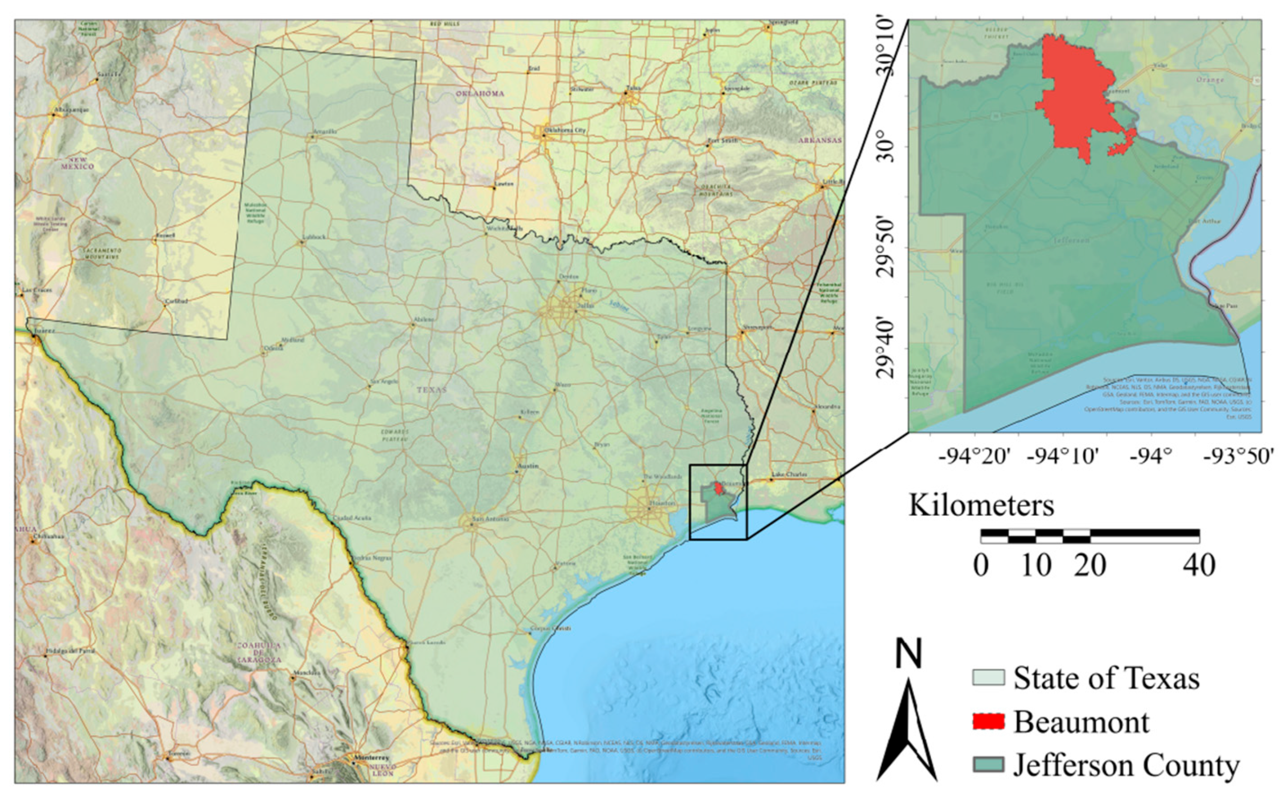
Beaumont, a coastal city near the Gulf of Mexico located in Southeast Texas, offers a strategic location due to its well-developed drainage network and the availability of flood sensors. This city, with a population of 112,193 people as of 2023, experiences an average monthly high temperature of 33.9 °C in August and an average monthly low temperature of 5.6 °C in December and January. The city is located on the western bank of the Neches River, with an average elevation of 6.10 m. June is the wettest month in Beaumont, with an average monthly precipitation of 182.8 mm, and April is the driest month, with an average monthly precipitation of 74.2 mm. The city’s flat topography, the strategic placement of sensors by the Southeast Texas Flood Control Division and Jefferson County Drainage District 6 (DD6) in critical areas, and a developed drainage and ditch network further enhance its suitability as a study site. By focusing on Beaumont, this research seeks to fill a critical data gap in the region while demonstrating the potential of satellite-based methods in improving the accuracy of nuisance flood mapping (Figure 2).

2. Materials and Methods

The main objective is to use the TCI, which was derived from topographic analysis together with water pixel concentrations, and the flood frequency map derived from Radar image analysis, to determine the area of concern for frequent flooding. Statistical analysis to find the relationships between the TCI and water pixel concentration and the flood frequency map.

2.1. Topographic Analysis to Generate TCI

A 1 m LiDAR Digital Elevation Model (DEM) for Beaumont was downloaded from the Texas Natural Resources Information System (TNRIS) [21,22] and mosaiced. The DEM was clipped to the city boundary and processed using ArcGIS Pro 3.0.0’s general fill tool. Depressions were identified by subtracting the original DEM from the filled DEM. Afterwards, the depressions were reviewed and only depressions > 12,000 m² with depths > 10 cm were included, yielding 378 depressions. Using the D8 algorithm in ArcGIS Pro 3.0.0, flow direction, accumulation, and watershed boundaries were determined (from the outlet point of depression), along with the average slope of catchments (Figure 2). Inundation volumes were estimated for depressions at 10 cm depth to calculate the TCI (Equation (1)):

$$\mathrm{TCI} = Ln\left({\displaystyle \frac{R \times A \times \sqrt{S}}{V}}\right)$$

(1)

where R is the unit inundation water depth (generally 1), A is the catchment area of the depression, S is the average slope, and V is the ponding volume [20]. Figure 3 is an example of a depression area plan view and section from A to A′, and area B is the portion potentially inundated to 10 cm.

2.2. Radar Image Analysis for Water Pixel Detection

To identify water pixels based on Radar imagery, a rainfall analysis should be conducted to find the most suitable image based on the wet days and time. To identify wet days, a comparison was made between PRISM precipitation data and the current water stage sensors. Based on the precipitation data from PRISM, only those days were selected in which there was also a water level rise in the available ground flood monitoring sensors (Algorithm 1).

Daily precipitation data from Parameter-elevation Regressions on Independent Slopes Model (PRISM) Climate Group (14 June 2014 to 6 July 2024) were collected at a 4 km resolution across 18 grids covering the city to analyze frequent flooding in Beaumont, Texas. Rainfall was categorized into four thresholds (<3 cm, 3–10 cm, 10–20 cm, and >20 cm in 24 h), with 3–10 cm events defined as significant for further analysis. Radar images corresponding to these rainfall events were downloaded from the Alaska Satellite Facility’s webpage [23].

In addition, the city of Beaumont has installed several flood monitoring sensors within the city area [19]. Water elevation data from these sensors can be found at SETX Rain. This information was used to further assess the six days during which the radar images were valid by seeing if at least one of the flood sensors in Beaumont’s five regions (North-East, South-East, South-West, North-West, and Central) recorded a significant stage rise on those days.

Finally, a total of six wet dates that meet these criteria were selected and compared with dry days for generating a water pixel concentration map. After selecting the dates, radar images from Sentinel-1A C-band Interferometric Wide (IW) Swath Ground Range detected High-Resolution data (GRDH) were processed using the European Space Agency’s Sentinel Application Platform (SNAP) software (Version 9.1) [24] and GIS tools [14,25]. The orbit file was used initially for precise geocoding so that the satellite position and velocity information were accurate at the time of image acquisition. The data were then subset to the Beaumont extent, and a land-sea mask limited the image to the city’s boundaries. Radiometric image calibration normalized backscatter values using an absolute calibration constant during Level 1 product generation. Speckle filtering followed, using a Lee filter (3 × 3) to remove noise caused by out-of-phase wave interactions. Range Doppler Terrain Correction addressed geometric distortions from viewing angles and high-rise structures [26,27]. Afterward, land elevation data (SRTM 1 sec HGT) were incorporated, and a band equation (Sigma0_VV < 0.05 & elevation < 10) was applied to extract regions below 10 m with low backscatter. The process was repeated for dry days, and a raster calculator in QGIS [28] subtracted dry-day data from wet-day data, identifying water pixels only present on wet days (value = 1). This method was applied to six events, and the results were aggregated into a flood frequency map.

Algorithm 1. Wet day selection algorithm
Select rainy days from the precipitation dataset. Check whether those rainy days also show a water-level rise in ground flood monitoring sensors.
	If yes → proceed. If no → discard.
For the remaining days, check whether radar imagery is available.
	If radar imagery exists → keep the date. If not → remove the date.

Ragdar Imagery Validation

To verify the accuracy of the Sentinel-1 radar-derived flood maps, ground-based water level sensors were used. A 20 m × 60 m rectangular buffer was generated around each sensor, and the presence of water pixels inside this area during each wet event was compared with the sensor’s stage data. Classification was defined as follows:

• True Positive (TP): at least one water pixel is detected and the sensor stage > 0.
• False Positive (FP): water pixels are detected, but the sensor stage ≤ 0.
• False Negative (FN): no water pixels are detected, but the sensor stage > 0.
• True Negative (TN): no water pixels are detected, and the sensor stage ≤ 0.

Using these outcomes, precision, recall, F1-score, and accuracy (Equations (2)–(5)) were calculated to quantitatively assess radar performance. These metrics range from 0 to 1, with higher values indicating better agreement between radar-detected water presence and ground sensor observations:

$$\mathrm{Precision} = {\displaystyle \frac{\mathrm{T}\mathrm{P}}{(\mathrm{T}\mathrm{P}+\mathrm{F}\mathrm{P})}}\times 100$$

(2)

$$\mathrm{Recall}={\displaystyle \frac{\mathrm{T}\mathrm{P}}{(\mathrm{T}\mathrm{P}+\mathrm{F}\mathrm{N})}}\times 100$$

(3)

$$\mathrm{F}1-\mathrm{score}={\displaystyle \frac{(2\times \mathrm{P}\mathrm{r}\mathrm{e}\mathrm{c}\mathrm{i}\mathrm{s}\mathrm{i}\mathrm{o}\mathrm{n}\times \mathrm{R}\mathrm{e}\mathrm{c}\mathrm{a}\mathrm{l}\mathrm{l})}{(\mathrm{P}\mathrm{r}\mathrm{e}\mathrm{c}\mathrm{i}\mathrm{s}\mathrm{i}\mathrm{o}\mathrm{n}+\mathrm{R}\mathrm{e}\mathrm{c}\mathrm{a}\mathrm{l}\mathrm{l})}}\times 100$$

(4)

$$\mathrm{Accuracy}={\displaystyle \frac{\mathrm{T}\mathrm{P}+\mathrm{T}\mathrm{N}}{(\mathrm{T}\mathrm{P}+\mathrm{T}\mathrm{N}+\mathrm{F}\mathrm{P}+\mathrm{F}\mathrm{N})}}\times 100$$

(5)

where TP = True positive (correctly detected water pixels), TN = True negative (correctly detected non-water pixels), FP = water pixels in the flood map but non-water pixels in the sensor, and FN = non-water pixel in the flood map but water pixels as observed pixels. Although metrics like root mean square error and average difference are available for accuracy assessment, they become less informative as they measure squared error rather than true positives and true negatives. Thus, the four selected metrics can be considered for accuracy evaluation.

2.3. Statistical Analysis

After generating the map of depressions with their respective TCI indices and developing a flood frequency map, the intensity of flood occurrence inside and outside of all depressions is statistically discussed to understand the relation between the TCI and flood frequency map and the relation between the water pixel concentration inside and outside of depressions (Equation (6)):

$$Water Pixel Concentration=\left({\displaystyle \frac{N_{water}}{N_{water} +{ N}_{non water}}}\right) \times 100$$

(6)

where

• $N_{\mathrm{water}}$ = number of water pixels detected in the radar image;
• $N_{\mathrm{non}-\mathrm{water}}$ = number of non-water pixels in the radar image.

Two non-parametric methods were employed for statistical analysis: Friedman test (Equation (7)) and the sign test (Equation (8)) [22,23,24]. Non-parametric methods were chosen because the pixel data were skewed, with an unknown distribution, unequal variances, and potential outliers, conditions under which parametric tests requiring normality are not suitable [28,29]:

$$\mathrm{F}\mathrm{r}\mathrm{i}\mathrm{e}\mathrm{d}\mathrm{m}\mathrm{a}\mathrm{n}\mathrm{’}\mathrm{s} \mathrm{C}\mathrm{o}\mathrm{e}\mathrm{f}\mathrm{f}\mathrm{i}\mathrm{c}\mathrm{i}\mathrm{e}\mathrm{n}\mathrm{t}=\left({\displaystyle \frac{12}{nk\left(k+1\right)}}\sum _{j=1}^k{R}_j^2\right)-3n\left(k+1\right)$$

(7)

$$\begin{array}{c}p-\mathrm{v}\mathrm{a}\mathrm{l}\mathrm{u}\mathrm{e}=2\times \mathrm{P}(\mathrm{X}\le \mathrm{x})\\ \mathrm{P}(\mathrm{X} \le \mathrm{x})={\sum }_{x=0}^n\left({\displaystyle \genfrac{}{}{0pt}{}{n}{x}}\right){0.5}^x\end{array}$$

(8)

where x is the smaller of the positive and negative differences and n is the number of observations.

The Friedman test (Equation (7)) is a non-parametric alternative to ANOVA for analyzing mean rank differences in more than two dependent groups. The sign test is a non-parametric approach used when t-test conditions are unmet [30]. It evaluates the statistical significance of a distribution assumption [30]. These tests are conducted at a chosen significance level, and conclusions are drawn based on the p-value. While the Friedman test may be utilized in multiple groups, the sign test may be utilized in a two-group comparison.

3. Results and Discussion

3.1. Topographic Result

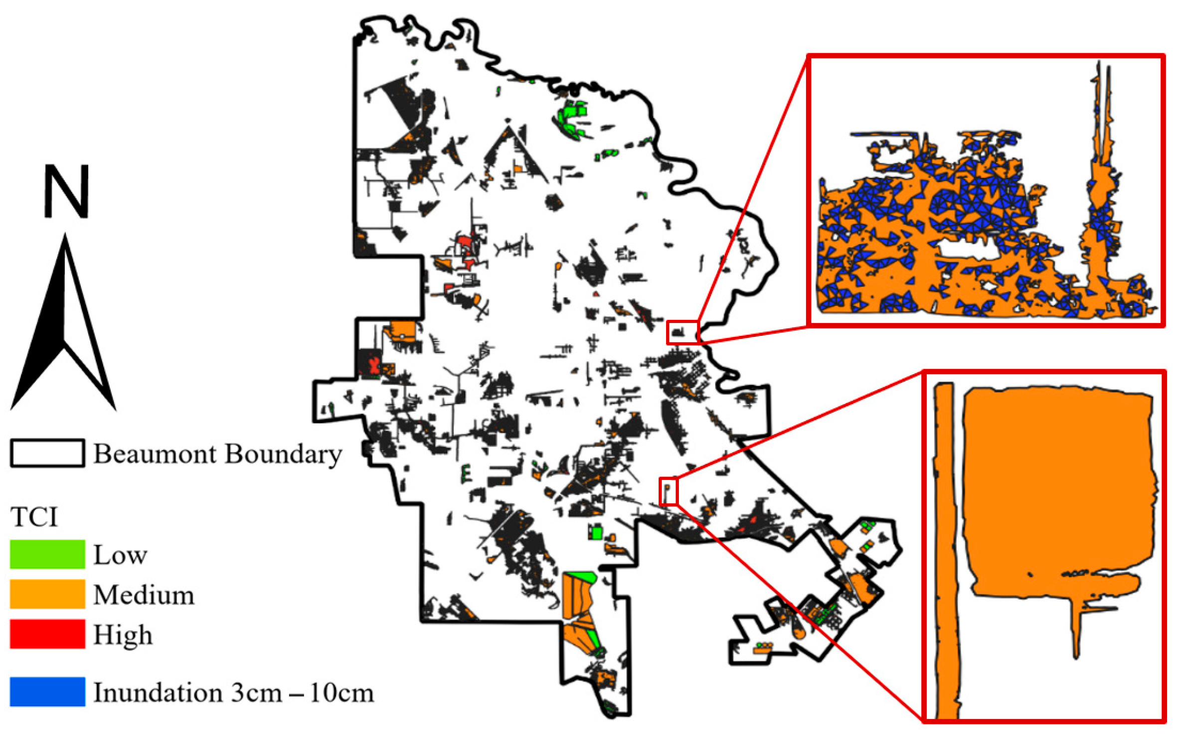
A total of 378 depressions were identified, filtered by areas > 12,000 m² and depth of >10 cm. The TCI was categorized into Low, Medium, and High groups based on the mean (11.21) and standard deviation (2.86) of the TCI values. Depressions with “TCI < mean − standard deviation” were classified as Low, and the “TCI > mean + standard deviation” were considered as High TCI, and the rest as Medium TCI. The TCI map was compared with Beaumont’s two-year flood inundation map. Among the identified depressions, 86 were outside the study zone of the two-year flood inundation map. Of the 292 depressions within a flood depth range of 3–10 cm, 246 (84.25%) overlapped with the inundation map. Figure 4 illustrates these overlaps, including a zoomed section showing Medium TCI depressions with and without overlap. The comparison highlighted a strong correlation between TCI values and areas with water inundation of 3–10 cm, confirming the TCI’s effectiveness in identifying flood-prone areas.

3.2. Flood Frequency Mapping Using Sentinel-1 Radar Imagery

Water elevation (stage) data from flood monitoring sensors were analyzed to understand the relationship between peak water levels and those at Sentinel-1 image acquisition times, along with the time elapsed between these events. Table 1 highlights the average time difference and the average percentage change in water levels (Equation (9)) at image acquisition time:

$$\% Change in Water Level=\left({\displaystyle \frac{H_{peak}-H_{acq}}{H_{peak}}}\right) \times 100$$

(9)

where

• $H_{\mathit{peak}}$ = peak (maximum) water level during the event;
• $H_{\mathit{acq}}$ = water level at the radar image acquisition time.

Table 1. Properties of the radar image in comparison with the peak of rainfall events.

Wet Dates	Mean Delta T (h)	Mean % Change in Water Levels (%)	Number of Active Sensors
19 April 2016	10.11	10.95	11
20 January 2017	6.01	8.67	6
16 June 2021	4.37	13.79	16
10 July 2021	4.26	10.89	19
25 January 2023	6.31	38.27	39
12 June 2024	2.99	17.03	38

Table 1. Properties of the radar image in comparison with the peak of rainfall events.

Wet Dates	Mean Delta T (h)	Mean % Change in Water Levels (%)	Number of Active Sensors
19 April 2016	10.11	10.95	11
20 January 2017	6.01	8.67	6
16 June 2021	4.37	13.79	16
10 July 2021	4.26	10.89	19
25 January 2023	6.31	38.27	39
12 June 2024	2.99	17.03	38

The average time difference was 5.7 h, and the average percentage difference was 16.6%. Table 1 presents data from active water level sensors for six wet days in Beaumont, revealing a significant increase in the number of sensors recording stage data after 2021. Some sensors failed on wet days, reducing the number of active sensors. Observations indicate that radar images were generally acquired within 6 h after peak depth was observed, with the water level 16% lower than at peak time. Only six images were taken on the same day near the peak of 159 flooding events (3–10 cm rainfall in 24 h) from 2014 to 2024, resulting in a low data acquisition rate (<4%).

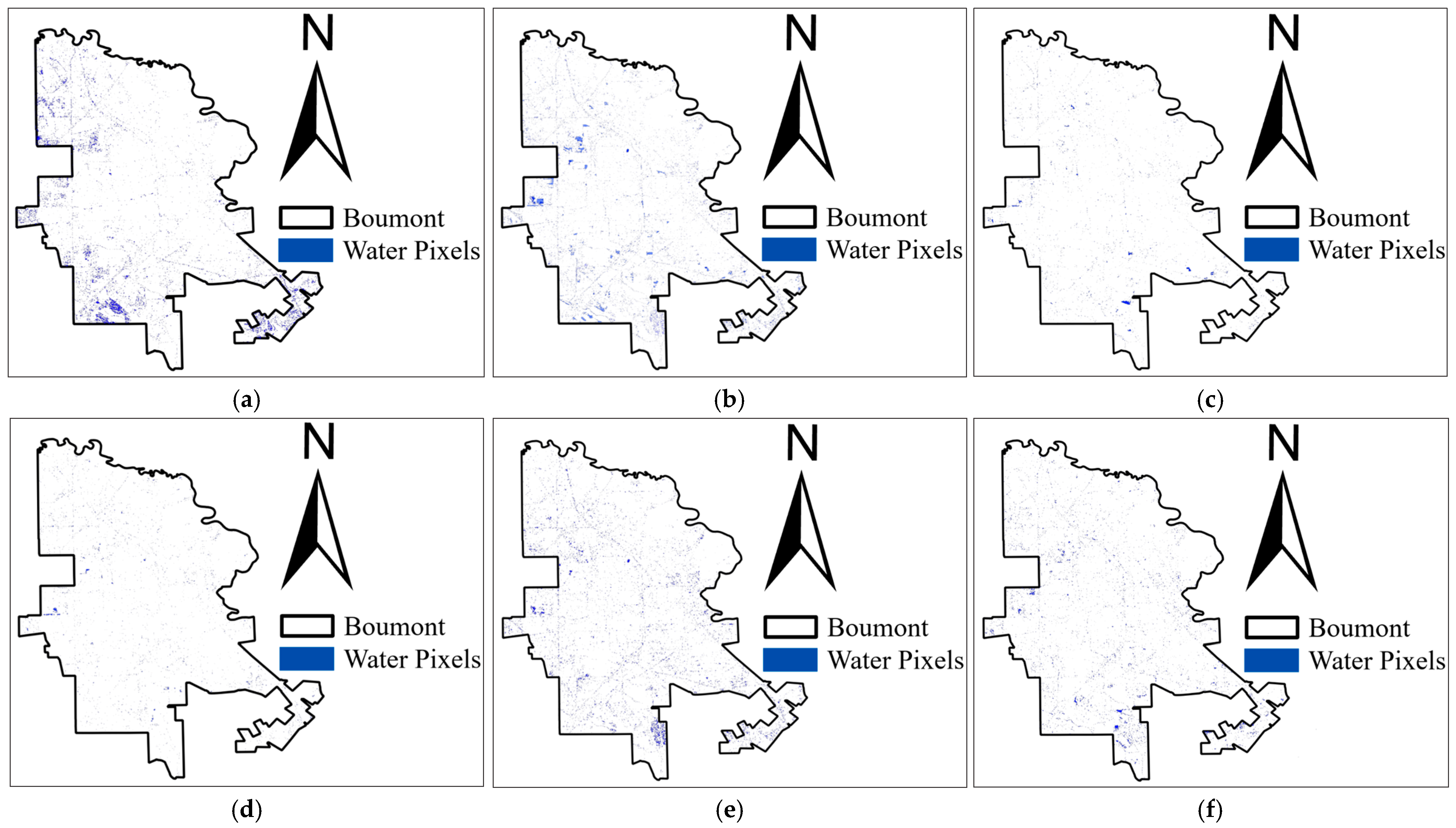
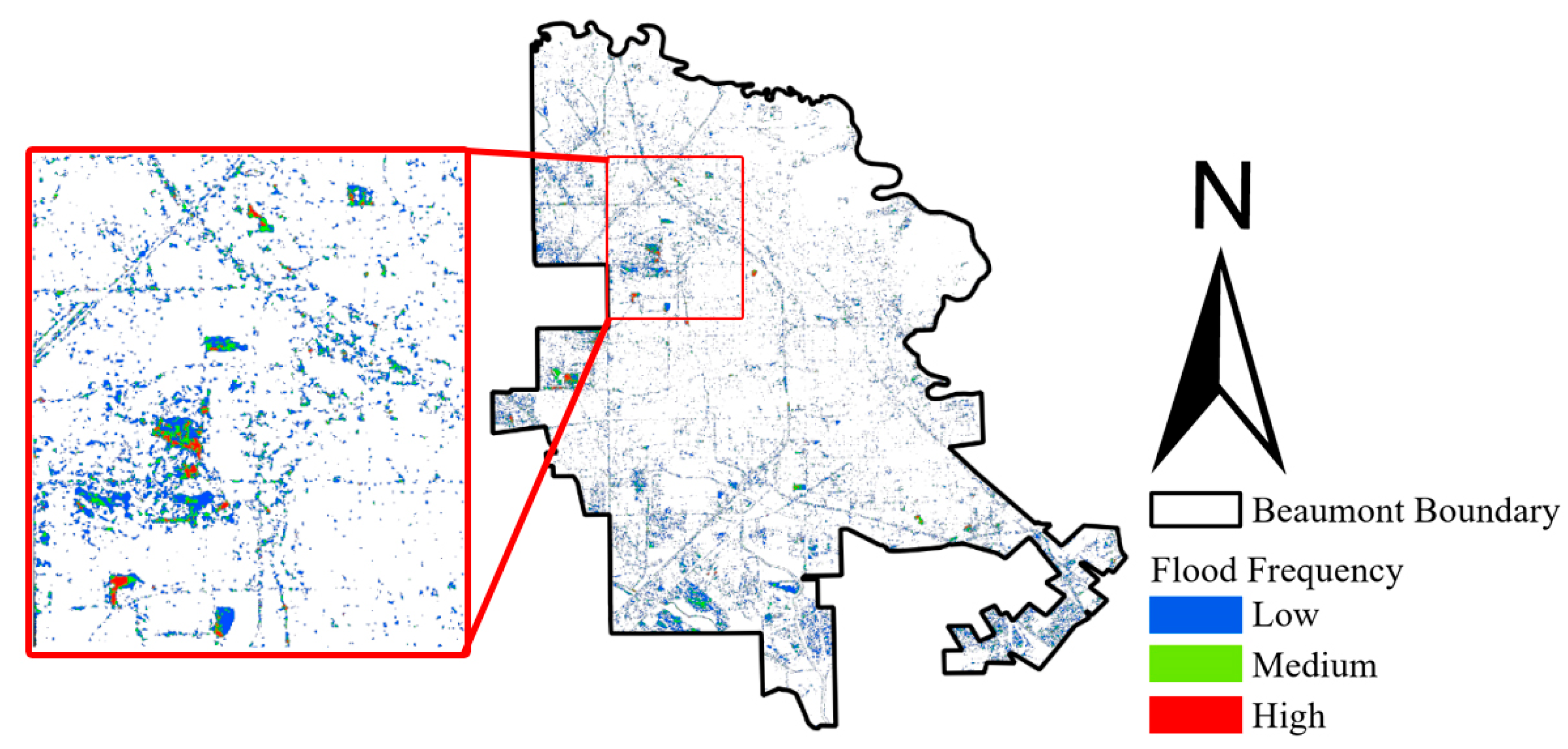
Water pixel maps prepared from radar images for six rainfall events are shown in Figure 5. All six events were combined, and a frequency map was generated and shown in Figure 6. The pixels that only have 1 water pixel are considered low, 2 water pixels overlapping are medium, and 3 or more water pixels overlapping are considered high frequency in this study. The frequency map shows that western Beaumont experiences more pluvial flooding than the eastern side. Southern Beaumont faces more flooding events compared to the north.

3.2.1. Validation of Radar Imagery Using Sensors

The flood maps were validated using a network of 49 water level sensors (as of 2024) installed by Drainage District 6 (DD6) and the Southeast Texas Flood Control District [19]. Validation was performed using four metrics: precision, recall, F1-score, and accuracy (Equations (1)–(4)). Sensor readings were classified as True Positive, True Negative, False Positive, and False Negative. No false positives were observed in the study.

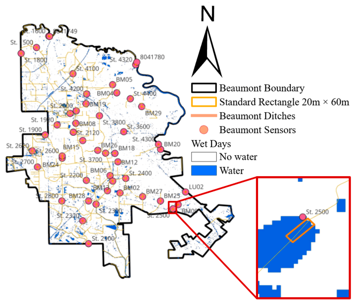
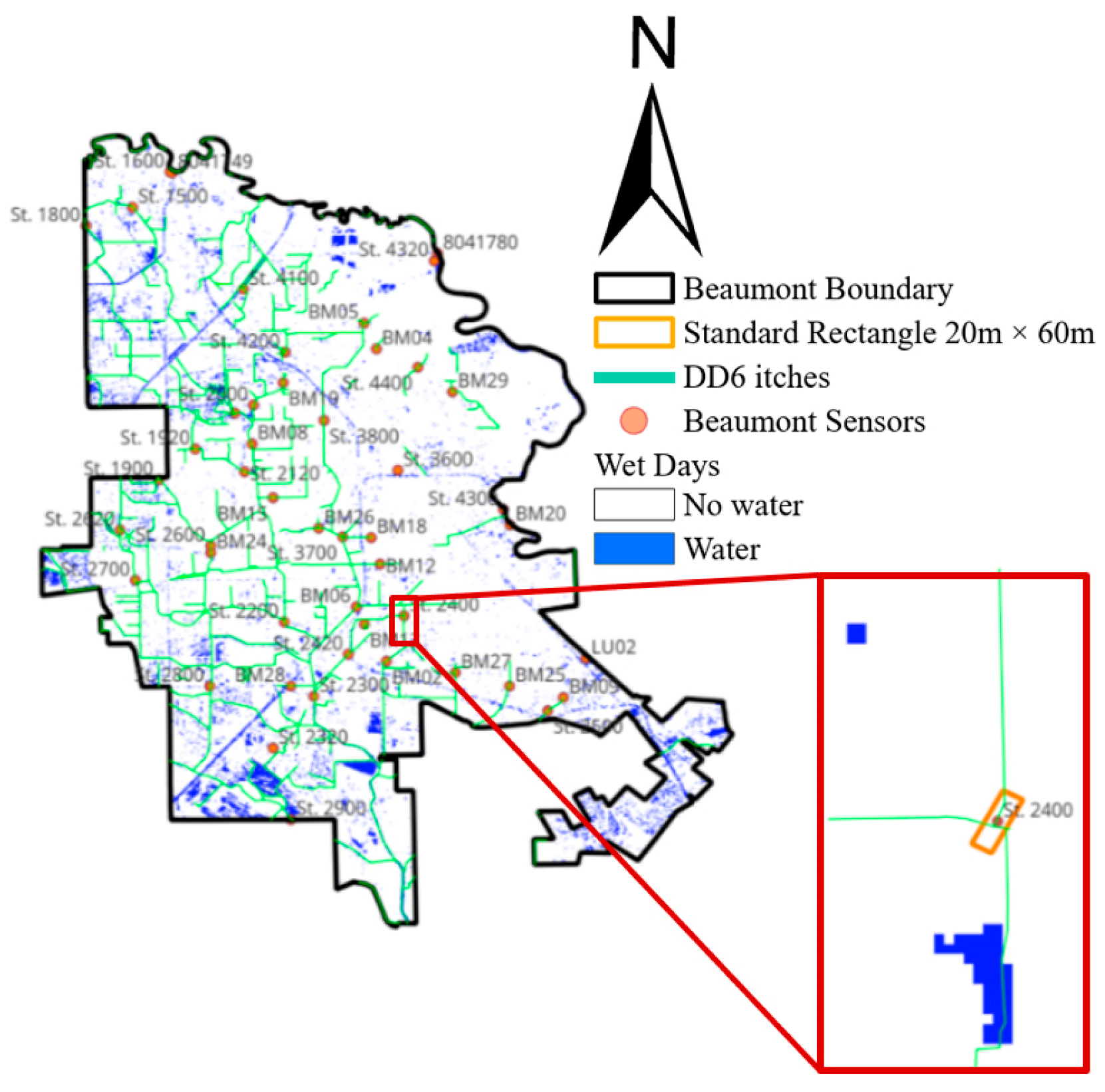
The sensor named St. 2500, with a stage of 8.29 ft and water pixels in the standard rectangle (20 m × 60 m), was classified as True Positive. Sensor St. 2400, with a stage of 6.22 ft but no water pixels in the standard rectangle, was a False Negative. Sensor BM04, with a stage of 0 ft and no water pixels in the rectangle, was classified as a True Negative. Figure 7, Figure 8 and Figure 9 illustrate these results.

The confusion matrix (

Table 2. Confusion Matrix of Radar Image on Wet Day and Sensor Data.

Radar Image|Sensor Stage	Stage > 1 In	Stage < 1 In
Number of Sensors surrounded by water pixels in radar image	90 (True Positive)	0 (False Positive)
Number of Sensors not surrounded by water pixels in radar image	37 (False Negative)	2 (True Negative)

) showed 90 true positives, 37 false negatives, 2 true negatives, and 0 false positives. The precision was 100% which can indicate that all predicted positive observations were accurate. Recall was 70.87%, showing strong identification of positive observations among all cases. The F1-score of 82.95% can be considered as a good balance between precision and recall. Accuracy was 71.32%, indicating correct predictions among watered pixels around sensors (

Table 3. Performance Metrics of Radar Images Against Sensor Data.

Performance Metrics	Value (%)
Precision	100
Recall	70.87
F-1 score	82.95
Accuracy	71.32

).

3.2.2. Identification of Pluvial Nuisance Flooding Hotspots

The number of water pixels from all 6 Sentinel-1 images was counted inside each depression area. The percentage of the area occupied by water pixels inside the depression compared to the area of the depression shows the sensitivity of that depression area. The result of this water pixel concentration is categorized into 6 groups: No water, Extremely Low (0–6%), Low (6–16%), Medium (16–38%), High (38–55%), and Extremely High (>55%).

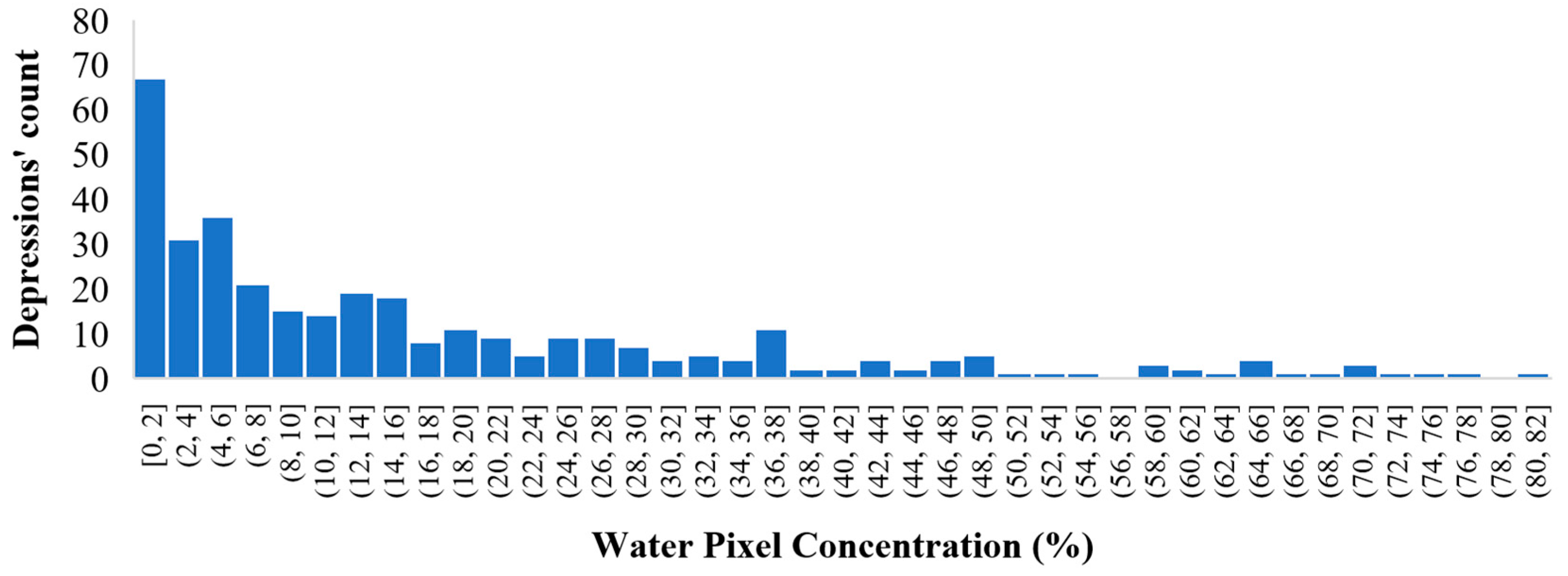
Figure 10 categorizes the number of depressions according to the percentage of water concentration within each depression area. It also indicates that the overall water concentration in the Beaumont area, excluding the depression zones, is 8.66%. Out of 378 depressions, 131 exhibited extremely low water concentrations, indicating effective drainage within six hours of peak rainfall. In Beaumont, 89 depressions had low water concentrations, 83 had medium, 22 had high, and 19 had extremely high water concentrations.

Out of 378 depressions, 124 retained significant water (medium to extremely high water pixel concentration) six hours after peak rainfall. Among these, 97 depressions (78%) had medium or high TCI values, confirming that areas with steeper contributing slopes and limited storage capacity are more prone to post-rainfall ponding. This strong correlation validates TCI as a reliable indicator for detecting flood-susceptible terrain (

Table 4. Water pixel concentration distribution within depressions classified by TCI.

		Water Pixel Concentration
		No Water	Extremely Low	Low	Medium	High	Extremely High
TCI Class of Depression	Low	10	11	11	21 (1)	3	3 (1)
	Medium	21	98	62 (4)	55 (5)	19 (5)	13 (7)
	High	3	22	16	7 (3)	0	3 (3)

Note(s): Values in the parentheses show the number of detention ponds in each TCI-water pixel concentration category.

).

Detention ponds were primarily located within the medium and high-TCI classes and corresponded to high or extremely high-water pixel concentrations. These engineered structures intentionally retain water during storm events and therefore do not indicate drainage failure. A total of 25 detention ponds were identified among the 124 medium to extremely high water pixel concentrated depressions, reflecting proper flood-control design and confirming good alignment between the modeled TCI and actual drainage performance. After excluding detention ponds, 99 natural depressions remained that exhibited medium-to-extremely-high water concentrations. These natural, non-engineered depressions are the true indicators of flood vulnerability. Of these, 74 depressions have medium or high TCI, showing that they are topographically predisposed to rapid inflow and poor drainage, making them the highest flood-mitigation priority (Figure 11).

Such depressions are ideal candidates for mitigation through culvert enlargement, local regrading, small detention retrofits, or the installation of green infrastructure such as bioswales or infiltration basins. Conversely, low-TCI depressions displayed mostly low or extremely low water pixel concentrations, indicating strong infiltration and effective natural drainage.

Figure 12 shows urban pluvial flooding hotspots characterized by significant water pixel concentrations and medium-to-high TCI values. After excluding areas with expected or controlled flooding such as natural water bodies, detention ponds, and designated flood-control zones. These locations represent zones of uncontrolled urban flooding risk. These included areas near Beaumont Municipal Airport, the neighborhood between Seale Rd and Chapel Ln, the exit from E Cardinal Drive to SML King Jr Pkwy, SML King Jr Pkwy from Neches St to East Elgie St, the neighborhood between Finnis Street and Schwarner Street, and the commercial zone of College Street from 8th Street to Private Road (Figure 13).

3.3. Statistical Results

3.3.1. Comparison of the Flood Frequency Map with Depression

The flood frequency map was compared with the TCI map to evaluate differences in water pixel concentrations across depressions categorized as low, medium, and high TCI. The statistical significance of water pixel concentrations within and outside all depressions was analyzed.

3.3.2. Comparison of Flood Frequency Map Within the Depressions (Friedman Test)

Water pixel concentration in all depressions where studied. Based on the intensity of flood frequency (low, medium, high, Null) and the TCI index of each depression, 3 groups of results have been classified from low to high, and 1 group (group 4) has been defined for those depressions with no water pixels. The percentage of flood frequency in each group is presented in

Table 5. Flood frequency percentage inside the depressions.

		TCI
		Low	Medium	High
Flood frequency	Low	16.54%	12.04%	11.29%
	Medium	4.50%	2.94%	4.04%
	High	1.58%	0.83%	1.63%
	Null	77.38%	84.19%	83.04%
Null Hypothesis: There is no significant association between the proportion of low, medium, high, and Null flood frequency and the TCI. Alternative Hypothesis: There is a significant association between the proportion of low, medium, high, and Null flood frequency and the TCI.

. Water Pixels repeated once in six events were labeled “low,” those repeated in two events as “medium,” and those repeated three or more times as “high.” Pixels without water in all six events were “Null”.

A Friedman test was employed on the data presented in Table 4, and the result was the Friedman coefficient of 0.5 and p-value of 0.779, indicating there is no significant association between pixel concentration percentage categories and TCI groups at the 5% significance level.

Because the radar images were acquired within six hours of peak flooding, the absence of a significant association is likely due to the timing of image acquisition relative to the flood peak. Water drainage from depressions during this period may have led to low water pixel concentrations in some cases. The presence of 70 depressions with <1% water concentration supports this explanation.

3.3.3. Comparison of Flood Frequency Map Inside and Outside the Depressions (Sign Test)

Table 6. Mean and Median Water Pixel Concentration Inside and Outside the Depressions.

Depressions/Pixels	Mean Water Pixel Concentration (%)	Median Water Pixel Concentration (%)
Inside depressions	16.67	8.16
Outside depressions	8.66	8.66
Null Hypothesis: The median of the differences between the water pixels inside and outside is equal to 0. Alternative Hypothesis: The median of the differences between the water pixels inside and outside is not equal to 0.

indicates that the average overall water pixel concentration inside depressions (16.67%) is nearly double that outside (8.66%). Among individual depressions, 34 depressions had no water pixels, and 36 depressions had <1% water concentration, with a range of 0% to 80.75%. The median concentration within depressions was 8.16%.

A sign test was employed to determine the median difference in water pixel concentration inside and outside depressions. The number of positive differences is all depressions with Higher than the Median water pixel concentration percentage outside the depression, and negative differences are all depressions lower than the median water pixel concentration percentage outside the depression (

Table 7. Summary of Sign Test Inside and Outside the Depression.

Description	Count
Total number of depressions	378
Number of positive differences	186
Number of negative differences	192
Number of ties	0

).

The null hypothesis stated that there was no difference between water pixel concentrations inside and outside the depressions, while the alternative proposed that a difference existed. The p-value of 0.797 indicated that the null hypothesis could not be rejected, confirming that no statistically significant difference was observed between the two Water pixel concentrations inside and outside the depressions. Despite this, the higher overall concentration inside depressions is evident, though the median difference was 0. This outcome was influenced by many depressions with negligible water concentration due to post-peak drainage within six hours of rainfall events. In general, while the water concentration inside depressions is higher on average, the timing of image acquisition and water drainage dynamics reduced the statistical differences in the sign test results.

4. Conclusions

This study assessed the use of Sentinel-1 radar imagery and the Topographic Control Index (TCI) to map flood frequency and identify urban pluvial flooding hotspots in Beaumont, Texas. Radar-based flood (water pixel) maps were validated using ground-based flood monitoring sensors by comparing radar-detected water presence with the sensors’ recorded stage values. The validation showed a precision of 100%, a recall of 70.87%, and an F1-score of 82.95%, confirming that radar imagery reliably identifies water that remains in poorly drained areas, although short-duration floods were missed due to delayed image acquisition.

Out of 378 depressions, 124 retained significant water six hours after peak rainfall, and 97 of these (78%) had medium or high TCI values. Water concentration in depressions (16.67%) was nearly double that outside (8.66%), and about 84% of medium-to-high TCI areas overlapped with existing two-year flood inundation maps. After excluding engineered detention ponds, 99 natural depressions were identified as flood-vulnerable zones, with 74 medium-to-high TCI depressions representing the priority areas for flood mitigation. These findings show that TCI is a reliable geomorphic indicator of flood vulnerability, even when short-term radar detection is affected by drainage timing.

This integrated approach can help city engineers and planners identify nuisance ponding areas, prioritize drainage network improvements, culvert redesigns, and permeable surface enhancements, and guide the placement of new flood sensors in high-risk locations. The results also highlight the value of engineered detention ponds and show where slow-draining natural depressions cause extended ponding.

The main limitation was the approximate six-hour lag between rainfall peaks and available radar images, which reduces visible water pixels and weakens the correlation between TCI and flood frequency. Future research should incorporate subsurface stormwater infrastructure, pipe capacity, and drainage connectivity to better represent flood dissipation and improve the relationship between radar-detected flooding and topographic indicators.

References

1. Ritchie, H.; Rosado, P.; Roser, M. Natural disasters. In Our World in Data; Global Change Data Lab: Oxford, UK, 2022. [Google Scholar]
2. Moftakhari, H.R.; AghaKouchak, A.; Sanders, B.F.; Matthew, R.A. Cumulative hazard: The case of nuisance flooding. Earths Future 2017, 5, 214–223. [Google Scholar] [CrossRef]
3. Moftakhari, H.R.; AghaKouchak, A.; Sanders, B.F.; Allaire, M.; Matthew, R.A. What is nuisance flooding? Defining and monitoring an emerging challenge. Water Resour. Res. 2018, 54, 4218–4227. [Google Scholar] [CrossRef]
4. Sweet, W.W.V.; Dusek, G.; Obeysekera, J.; Marra, J.J. Patterns and Projections of High Tide Flooding Along the US Coastline Using a Common Impact Threshold; National Oceanic and Atmospheric Administration (NOAA): Silver Spring, MD, USA, 2018. [Google Scholar]
5. Vega, A.J.; Miller, P.W.; Rohli, R.V.; Heavilin, J. Synoptic climatology of nuisance flooding along the Atlantic and Gulf of Mexico coasts, USA. Nat. Hazards 2021, 105, 1281–1297. [Google Scholar] [CrossRef]
6. Sweet, W.; Park, J.; Marra, J.; Zervas, C.; Gill, S. Sea Level Rise and Nuisance Flood Frequency Changes Around the United States; National Oceanic and Atmospheric Administration (NOAA): Silver Spring, MD, USA, 2014. [Google Scholar]
7. American Association of State Highway and Transportation Officials. A Policy on Geometric Design of Highways and Streets, 7th ed.; American Association of State Highway and Transportation Officials: Washington, DC, USA, 2018. [Google Scholar]
8. Justice, C.; Townshend, J.; Vermote, E.; Masuoka, E.; Wolfe, R.; Saleous, N.; Roy, D.; Morisette, J. An overview of MODIS Land data processing and product status. Remote Sens. Environ. 2002, 83, 3–15. [Google Scholar] [CrossRef]
9. Zhang, F.; Zhu, X.; Liu, D. Blending MODIS and Landsat images for urban flood mapping. Int. J. Remote Sens. 2014, 35, 3237–3253. [Google Scholar] [CrossRef]
10. Manjusree, P.; Prasanna Kumar, L.; Bhatt, C.M.; Rao, G.S.; Bhanumurthy, V. Optimization of threshold ranges for rapid flood inundation mapping by evaluating backscatter profiles of high incidence angle SAR images. Int. J. Disaster Risk Sci. 2012, 3, 113–122. [Google Scholar] [CrossRef]
11. Cossu, R.; Schoepfer, E.; Bally, P.; Fusco, L. Near real-time SAR-based processing to support flood monitoring. J. Real-Time Image Process. 2009, 4, 205–218. [Google Scholar] [CrossRef]
12. Oberstadler, R.; Hönsch, H.; Huth, D. Assessment of the mapping capabilities of ERS-1 SAR data for flood mapping: A case study in Germany. Hydrol. Process. 1997, 11, 1415–1425. [Google Scholar] [CrossRef]
13. Feizbahr, M.; Brake, N.; Arbabkhah, H.; Hariri Asli, H.; Woods, K. Flood Susceptibility Mapping Using Machine Learning and Geospatial-Sentinel-1 SAR Integration for Enhanced Early Warning Systems. Remote Sens. 2025, 17, 3471. [Google Scholar] [CrossRef]
14. Martinis, S.; Rieke, C. Backscatter analysis using multi-temporal and multi-frequency SAR data in the context of flood mapping at River Saale, Germany. Remote Sens. 2015, 7, 7732–7752. [Google Scholar] [CrossRef]
15. Huang, H.; Chen, X.; Wang, X.; Wang, X.; Liu, L. A depression-based index to represent topographic control in urban pluvial flooding. Water 2019, 11, 2115. [Google Scholar] [CrossRef]
16. Qi, M.; Huang, H.; Liu, L.; Chen, X. An integrated approach for urban pluvial flood risk assessment at catchment level. Water 2022, 14, 2000. [Google Scholar] [CrossRef]
17. Li, S.; Wahl, T.; Talke, S.A.; Jay, D.A.; Orton, P.M.; Liang, X.; Wang, G.; Liu, L. Evolving tides aggravate nuisance flooding along the US coastline. Sci. Adv. 2021, 7, eabe2412. [Google Scholar] [CrossRef] [PubMed]
18. Bureau, U.S.C. Quick Facts: Beaumont City, Texas. In United States Population Estimates; United States Department of Commerce: Washington, DC, USA, 2023. Available online: https://www.census.gov/quickfacts/fact/table/beaumontcitytexas/PST045223#PST045223 (accessed on 12 March 2024).
19. Asli, H.H.; Brake, N.; Kruger, J.; Haselbach, L.; Adesina, M. Field surveying data of low-cost networked flood sensors in southeast Texas. Data Brief 2023, 50, 109504. [Google Scholar] [CrossRef]
20. Qi, M.; Huang, H.; Liu, L.; Chen, X. Spatial heterogeneity of controlling factors’ impact on urban pluvial flooding in Cincinnati, US. Appl. Geogr. 2020, 125, 102362. [Google Scholar] [CrossRef]
21. Haselbach, L.; Adesina, M.; Muppavarapu, N.; Wu, X. Spatially estimating flooding depths from damage reports. Nat. Hazards 2023, 117, 1633–1645. [Google Scholar] [CrossRef]
22. USGS. Neches River Basin LiDAR. 2017. Available online: https://www.usgs.gov/centers/eros/science/neches-river-basin-lidar (accessed on 11 January 2024).
23. Alaska Satellite Facility. ASF Data Search (Vertex); Alaska Satellite Facility: Fairbanks, AK, USA, 2024. [Google Scholar]
24. European Space Agency. Sentinel Application Platform (SNAP), Version 9.1; European Space Agency: Paris, France, 2023.
25. Guo, H. Spaceborne and airborne SAR for target detection and flood monitoring. Photogramm. Eng. Remote Sens. 2000, 66, 611–617. [Google Scholar]
26. McVittie, A. SENTINEL-1 Flood Mapping Tutorial; SkyWatch Space Applications Inc.: Kitchener, ON, Canada, 2019; Available online: https://step.esa.int/docs/tutorials/tutorial_s1floodmapping.pdf (accessed on 23 March 2024).
27. Tanim, A.H.; McRae, C.B.; Tavakol-Davani, H.; Goharian, E. Flood detection in urban areas using satellite imagery and machine learning. Water 2022, 14, 1140. [Google Scholar] [CrossRef]
28. Pappas, P.A.; DePuy, V. An Overview of Non-Parametric Tests in SAS: When, Why, and How; Paper TU04; Duke Clinical Research Institute: Durham, NC, USA, 2004; pp. 1–5. [Google Scholar]
29. Zimmerman, D.W. A note on the influence of outliers on parametric and nonparametric tests. J. Gen. Psychol. 1994, 121, 391–401. [Google Scholar] [CrossRef]
30. Corrado, C.J.; Zivney, T.L. The Specification and Power of the Sign Test in Event Study Hypothesis Tests Using Daily Stock Returns. J. Financ. Quant. Anal. 1992, 27, 465–478. [Google Scholar] [CrossRef]
Figure 1. The study Framework for driving TCI and Generating Hotspots.
Water 17 03500 g001
Figure 2. Study area—Beaumont, Texas.
Water 17 03500 g002
Figure 3. Visualization of Catchment Area and Slope in TCI Calculation.
Water 17 03500 g003
Figure 4. TCI Map Overlaying the Existing Inundation Map with Depth 3 cm–10 cm.
Water 17 03500 g004
Figure 5. Radar images for six significant rainfall events. (a) Flood Map of 12 June 2024; (b) Flood Map on 25 January 2023; (c) Flood Map of 10 July 2021; (d) Flood Map on 16 June 2021; (e) Flood Map of 20 January 2017; (f) Flood Map on 19 April 2016.
Water 17 03500 g005
Figure 6. Flood frequency map of Beaumont, TX.
Water 17 03500 g006
Figure 7. True Positive Case on 12 June 2024.
Water 17 03500 g007
Figure 8. True Negative Case on 12 June 2024.
Water 17 03500 g008
Figure 9. False Negative Case on 12 June 2024.
Water 17 03500 g009
Figure 10. Number of Depressions vs. Water Pixel Concentration.
Water 17 03500 g010
Figure 11. Distribution of water concentration classes and Detention ponds in medium to extremely high-water pixel depressions.
Water 17 03500 g011
Figure 12. Depression at Lamar University Detention Pond. (a) Depressions with Detention Pond; (b) Depressions with Detention Pond overlaying Water Concentration; (c) Depressions with Water Pixels.
Water 17 03500 g012
Figure 13. Identified Flooding Spots Within Beaumont.
Water 17 03500 g013