Integrating Deep Learning and Copula Models for Flood–Drought Compound Analysis in Iran

Abstract

This study aims to forecast the combined impacts of drought and flood in the future using an integrated framework. This framework integrates U-Net++, quantile mapping (QM), Copula models, and ISIMIP3b gridded large-scale discharge data (1985–2014, 2021–2050, and 2071–2100). Copula models analyze compound effects in four dimensions to determine return periods for droughts and floods. The standalone U-Net++ and its integration with multiple linear regression, multiple nonlinear regression, M5 model tree, multivariate adaptive regression splines, and QM downscaled ISIMIP3b model river flows. U-Net++QM outperformed other models, with a 58% lower RRMSE. Ensemble GCMs showed less uncertainty than other models in river flow downscaling. For the Ensemble model, the highest drought severity was −300, the maximum duration was 300 months, flood peak flow reached 12,000 m³/s, and intervals lasted up to 22 months. Moreover, the return periods of compound events for this model ranged from 50 to 3000 years. Future river flow projections, using the Ensemble model and emission scenarios (SSP126, SSP370, and SSP585), showed increased vulnerability in 2071 and 2025 versus the observed period. Introducing an integrated framework serves as a management tool for addressing extreme combined phenomena under climate change.

1. Introduction

Droughts and floods cause considerable human and financial losses, especially in Iran. Inadequate rainfall distribution results in severe droughts and destructive floods, leading to significant economic, social, and environmental impacts.

Climate change has caused a 1.1–5.4 °C increase in temperature and changes in precipitation patterns [1]. This phenomenon has had a severe impact on Middle Eastern countries, especially Iran. Iran is experiencing a 2.6 °C increase in average temperature and a 35% decrease in precipitation [2]. Forecasting floods and droughts because of climate change is essential for effective planning. Accurate predictions rely on general circulation models’ data and emission scenarios, which require downscaling methods. Deep learning and machine learning can address these challenges, but identifying the most reliable global circulation model remains complex. Thus, uncertainty analysis is needed to assess forecast reliability.

Given the increasing impacts of drought and flooding on the development of human societies, various researchers have studied these phenomena and their relationships with climate change. Panagoulia and Dimou [3] studied the sensitivity of flooding to climate change in central Greece. The study reported that changes in precipitation, and subsequently, temperature have the greatest impact on flood occurrence and characteristics. Spatial and temporal variations in meteorological drought in a watershed in India was assessed using standardized indices and the inverse distance weighting method [4]. The results showed that the mentioned watershed had endured a severe drought in 1980. The impact of climate change on the frequency and severity of floods in the Kabul River basin in Afghanistan was assessed using the SWAT model under RCP scenarios [5]. The results indicated an increase in floods with a 1 to 50-year return period in the near future. The results of the RCP8.5 scenario also showed more severe droughts than the other two scenarios. The SRI and general circulation models, and SSP scenarios related to CMIP6 were used to predict hydrological drought under climate change conditions in China [6].

General circulation models are vital in water resource engineering, but their large scale limits direct use [7]. Recently, dynamical, statistical, and climate model methods have been developed to downscale these models, with statistical methods gaining popularity because of lower data requirements and acceptable accuracy [8]. These methods include linear and nonlinear regressions [9], machine learning algorithms [10,11], and some deep learning techniques [12]. Wilby et al. [13] developed SDSM 6.1 software using multivariate linear regression. According to the study of Harpham and Wilby [14], SDSM software is more accurate in downscaling precipitation than radial neural networks and multilayer perceptron neural networks. Wang et al. [12] used recurrent neural networks and traditional neural networks, as well as big data, to downscale precipitation, temperature, and hydrological modeling. The results showed that recurrent neural networks were more accurate than artificial neural networks. Balmaceda-Huarte et al. [15] performed a daily temperature downscaling of southern South America using convolutional neural networks. The results confirmed the CNN’s performance. Misra et al. [16] conducted a study on daily rainfall downscaling using a combination of convolutional neural networks and long short-term memory. The results showed that the method was more accurate than simple convolutional neural networks and long short-term memory networks. Cho et al. [17] used deep learning and spatial interpolation to downscale temperature data, achieving acceptable accuracy. Wang et al. [18] explored the combined effects of flood, drought, and land use on water quality. The results indicate that floods had a greater impact on water quality than droughts. The results of the study by [19] are based on a floods and droughts dataset from 1968 to 2020, the study highlighted the amplified negative impacts when droughts and floods occur concomitantly or sequentially. Xie et al. [20] used random forest and R-vine copula, and the combined effects of drought and drought–flood abrupt alternation on vegetation in China and Pakistan were investigated. Results from 1981 to 2019 indicate that drought events intensified, the risk of flood-to-drought decreased, and the risk of drought-to-flood increased.

In the country of Iran, Valikhan Anaraki et al. [21] used machine learning to downscale the general circulation models of the fourth and fifth reports to analyze flood frequency in the Karun 3 basin. Anaraki et al. [22] proposed a new method based on ensemble learning for precipitation downscaling. The results showed that the proposed method was more accurate than machine learning, such as least squares support vector machines and random forest. Ghafari and Parvishi [23] used an LSTM-based algorithm to project climate change in Lake Urmia. The results show increased severity and duration of droughts, especially in the 2040s and 2050s. Najafi et al. [24] study the spatial and temporal patterns of climate extremes in Iran. This study highlights the risk of more frequent and severe floods, particularly in the western, northern, and northwestern regions.

Based on the authors’ best knowledge, a gap exists in projecting the combined effects of drought and flood under climate change conditions. Although these phenomena typically occur at distinct intervals, climate change has compressed this timeline and intensified drought and flood events. A study conducted by [25] showed that in Iran, snow and warm-temperate climates experienced greater hydroclimatic changes than arid and semi-arid climate zones. The most noticeable trends were observed in temperature, which significantly increased across all counties, while drying trends were observed in precipitation, surface reservoir content, and runoff. Wind speed and surface albedo in most counties experienced upward and downward trends, respectively, whereas solar radiation, surface air pressure, and evaporation exhibited high spatial variability. Regarding extreme events, Iran experienced increased hot-climate extremes and decreased cold- and precipitation-related extremes. There is a threat to water resources management in Iran, which can increase the frequency and intensity of flood and drought events.

Hence, this research employs an integrated methodology to examine flood and drought as a compound event in Iran between 2021 and 2100. The U-Net++ architecture, combined with quantile mapping and machine learning, is used to downscale river flow data from the ISIMIP3b model. Subsequently, river flow projections are performed using the GFDL-ESM4, MRI-ESM2, and UKESM1-0-II models and emission scenarios (SSP126, SSP370, and SSP585), with uncertainties identified through fuzzy analysis. Copula functions are employed to evaluate the compound drought–flood phenomena in terms of drought intensity, flood peak flow, and multivariate return periods. The study investigates return periods, population growth, income variations, and changes in vulnerability across Iran related to these elements. Given the repercussions of climate change on water resources, the insights from this study will inform the formulation of effective long-term management and adaptation strategies.

2. Materials and Methods

This study first provides explanations about the case study and the data used. Then, the data-processing methods, machine learning and deep learning, drought analysis, flood analysis, the combination of drought and flood phenomena, copula functions, and evaluation criteria are presented.

2.1. Case Studies

This research focuses on Iran as a case study because of its regional and global significance. With over 86 million people and an area of 1,648,195 km², Iran is the second-largest country in the Middle East and the eighteenth-largest globally. Its unique geography—varying altitudes, coasts, forests, and extensive arid zones—creates diverse climates, ranging from extremely arid to very humid. Iran is classified into four climatic zones: the temperate and humid southern Caspian Sea coasts, the cold western mountains, the hot and arid central plateau, and the hot and humid southern coasts. 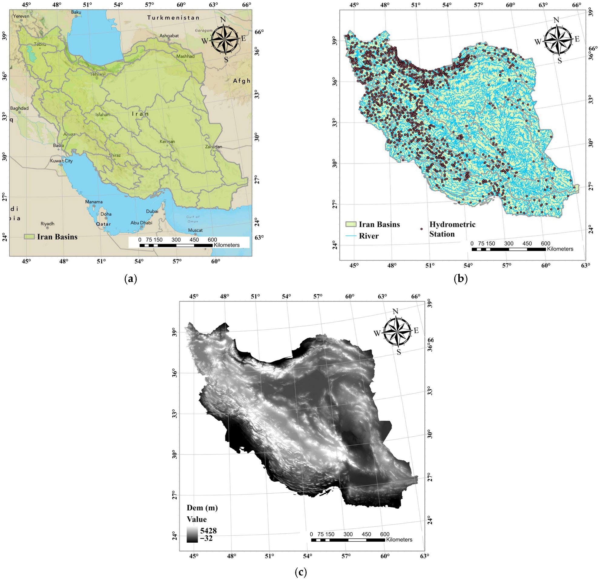Figure 1 shows Iran’s geographical position in the Middle East and its watersheds, segmented into 36 sections for this study based on data from the hydrosheds website. Also, in this figure, the river network, distribution of hydrometric stations, and digital elevation layer are observable. Based on this figure, almost all stations are in foothill regions. In these regions, the population is more concentrated, and access to water resources is greater.

2.2. Data Used

In this study, the grid flow dataset from ISIMIP3b in the base period (1966–2014) and the future period (2021–2100), and runoff observation data from hydrometric stations in the country in the base period are used as input data. The spatial resolution of ISIMIP3b data is 0.5° latitude by 0.5° longitude, and its time scale is daily. This river flow data have been generated using general circulation models and emission scenarios for the present and future periods. Different general circulation models, including GFDL-ESM4, MRI-ESM2-0, and UKESM1-0-LL, are investigated according to SSP126, SSP370, and SSP585 scenarios. The aforementioned models outperformed CNRM-CM6-1 and CNRM-ESM2, according to a study by [26]. Jiang et al. [27] reported that the MRI-ESM2-0 and UKESM1-0-LL models had a remarkable ability to forecast extreme precipitation. The GFDL-ESM4 model was selected as one of the efficient models in the precipitation forecasting study [28]. In addition, the use of the aforementioned models can help forecast precipitation under different conditions, given their different assumptions and specifications.

Table 1. Characteristics of the investigated general circulation models.

GCMs	Institutions	Variants
GFDL-ESM4	National Oceanic and Atmospheric Administration, Geophysical Fluid Dynamics Laboratory, USA	r1i1p1f1
MRI-ESM2-0	Meteorological Research Institute, Tsukuba, Japan	r1i1p1f1
UKESM1-0-LL	Met Office Hadley Centre, UK	r1i1p1f2

presents the specifications of the aforementioned general circulation models.

Table 2. Characteristics of the investigated climate change scenarios.

Abbreviation	Description	Challenges in Reducing Greenhouse Gas Emissions	Challenges in Adaptation
SSP126	Sustainable development scenario	Low	Low
SSP370	Regional rivalry scenario	Low	High
SSP585	Fossil fuel-driven development scenario	High	Low

outlines emission scenarios. In the first scenario, global CO₂ emissions sharply decline, achieving zero emissions after 2050 while stabilizing the temperature rise at about 1.8 °C by the century’s end. The SSP370 scenario sees escalating greenhouse gas emissions, with CO₂ nearly doubling by 2100, intensifying competition among nations, and prioritizing food security, resulting in a 3.6 °C temperature increase. In the SSP585 scenario, CO₂ emissions will also double by 2050, driven by rapid economic growth fueled by fossil fuels, leading to a catastrophic 4.4 °C rise by 2100. The first scenario is optimistic, the third pessimistic, with the second in between. Notably, adaptation challenges in the pessimistic scenario are low because of high economic growth, which reduces vulnerability to climate change risks and enhances adaptation opportunities.

In this study, observed runoff data from 1464 hydrometric stations were collected. The missing data of this dataset were estimated from the study of [25].

2.3. Quantile Mapping

The quantile mapping method is a statistical method for correcting bias in climate change predictions. This method determines the cumulative probability distribution function for the observed and predicted data. Then, the bias in the observed data is corrected using the following equation:

$$Y_{corrected}=CD{F}_{obs}^{-1}\left(CD{F}_{pred}\left(Y_{pred}\right)\right)$$

(1)

In Equation (1), $Y_{corrected}$ is bias-corrected data, ${CDF}_{obs}^{-1}$ is the inverse cumulative distribution function of observed data, ${CDF}_{pred}$ is the cumulative distribution function of predicted data, and $Y_{pred}$ is the predicted data. This method is used in many studies, such as [29,30].

2.4. Machine Learning Algorithms

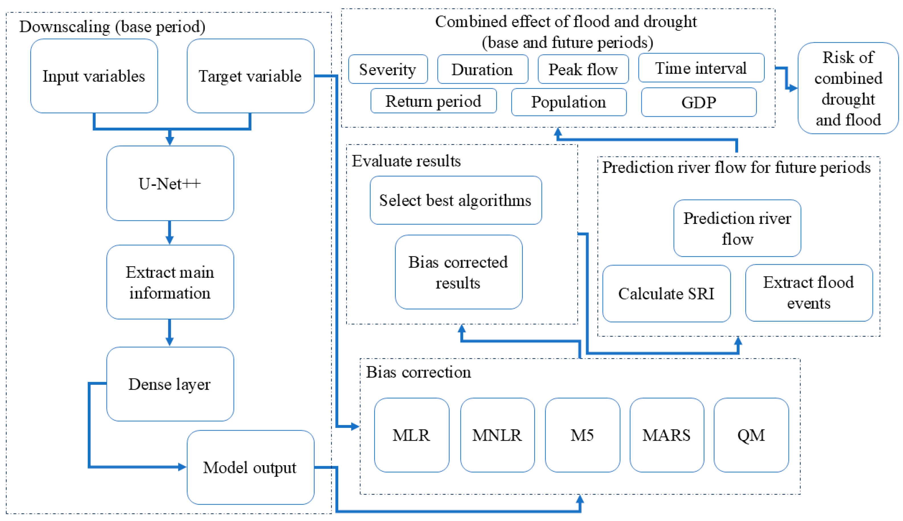
In this study, different machine learning algorithms are used to downscale river flow. The used algorithms include multiple linear regression (MLR), multiple nonlinear regression (MNLR), M5 model tree (M5), multivariate adaptive regression splines (MARSs), and quantile mapping (QM). These algorithms make different assumptions and using them can yield different results. MLR models the problem by assuming a linear relationship between the inputs and target data. MNLR operates by considering the nonlinear relationship between inputs and target data. In M5, the input data are partitioned into multiple clusters, and a linear regression is fit to each cluster. The MARS divides the input dataset into clusters and fits a nonlinear regression to each cluster. QM uses a probability approach to correct the distribution of input data. These algorithms can correct bias in U-Net++ outcomes. However, depending on the assumptions made, the results of bias correction can differ across the algorithms.

2.5. Multiple Linear Regression

MLR is a statistical method used for modeling and analyzing data. MLR models the output data as a linear function of the input data. MLR extends ordinary least squares regression by allowing more than one independent variable or attribute. MLR is an algorithm for examining the effect of a dependent variable by identifying relationships among the independent variables. The relationship between the inputs and the targets is assumed to be as follows:

$$Y=b_0+b_1\times X_1+b_2\times X_2+\dots +b_n\times X_n$$

(2)

In Equation (2), $Y$ is target variable, $X$ is the input variable, $b_0$ is bias, and $b_1$ to $b_n$ are inputs weights.

2.6. Multiple Nonlinear Regression

MNLR is a regression method for creating a nonlinear relationship between inputs and the target variable. This method is similar to MLR, except that it also considers the squares of the inputs. The nonlinear relationship between inputs and output in MNLR is determined based on the following relationship:

$$\begin{array}{l}Y=b_0+b_1\times X_1+b_2\times X_2+\dots +b_n\times X_n+\\ b_{n+1}\times X_{n+1}^2+b_{n+2}\times X_{n+2}^2+b_{n+3}\times X_{n+3}^2+\\ \dots +b_{2n}\times X_{2n}^2\end{array}$$

(3)

In Equation (3), $Y$ is known as the target variable, $X$ is related to the input variables, $b_0$ is bias, $b_1$ to $b_n$ are the weights of input variables, and $b_{\mathrm{n}+1}$ to $b_{2n}$ are the weights of the squared input variables.

2.7. M5 Model Tree

The M5 model tree is a parametric regression method that solves regression problems using the divide-and-conquer method. In this method, the original set of inputs is divided into several subsets; then, a linear regression relationship is fitted to each subset. The input decomposition process is carried out in several stages, like a decision tree. At each stage, there is a parent node and several child nodes. Parent nodes are datasets that are divided into several subsets (child nodes). After the tree is created, due to the large number of child nodes, the extra nodes are removed using the pruning method. This helps to prevent overfitting. The data division process continues until the criterion of the maximum reduction in the standard deviation is not less than a certain limit. This criterion can be calculated from the following relationship:

$$SDR=SD\left(T\right)-{\displaystyle \sum _{i=1}^N\frac{\left|T_i\right|}{\left|T\right|}}\times SD\left(T_i\right)$$

(4)

In Equation (4), $T$ is the parent node, $T_i$ is the child node, and $SD$ is standard deviation of the dataset.

2.8. Multivariate Adaptive Regression Splines

The MARS algorithm is designed to solve nonlinear regression and classification problems. In this algorithm, the dataset is divided into several subsets, and a nonlinear regression is fitted to each subset. This regression relation can be defined based on a basis function. The final equation to determine the relation between the inputs and outputs in the MARS algorithm is expressed as follows:

$$Y={\beta }_0+{\displaystyle \sum _{i=1}^N{\beta }_i\times BF\left(X\right)}$$

(5)

In Equation (5), ${\beta }_0$ is the bias coefficient, ${\beta }_i$ is the weight of the base function, and $BF$ is known as the base function.

2.9. Deep Artificial Neural Networks

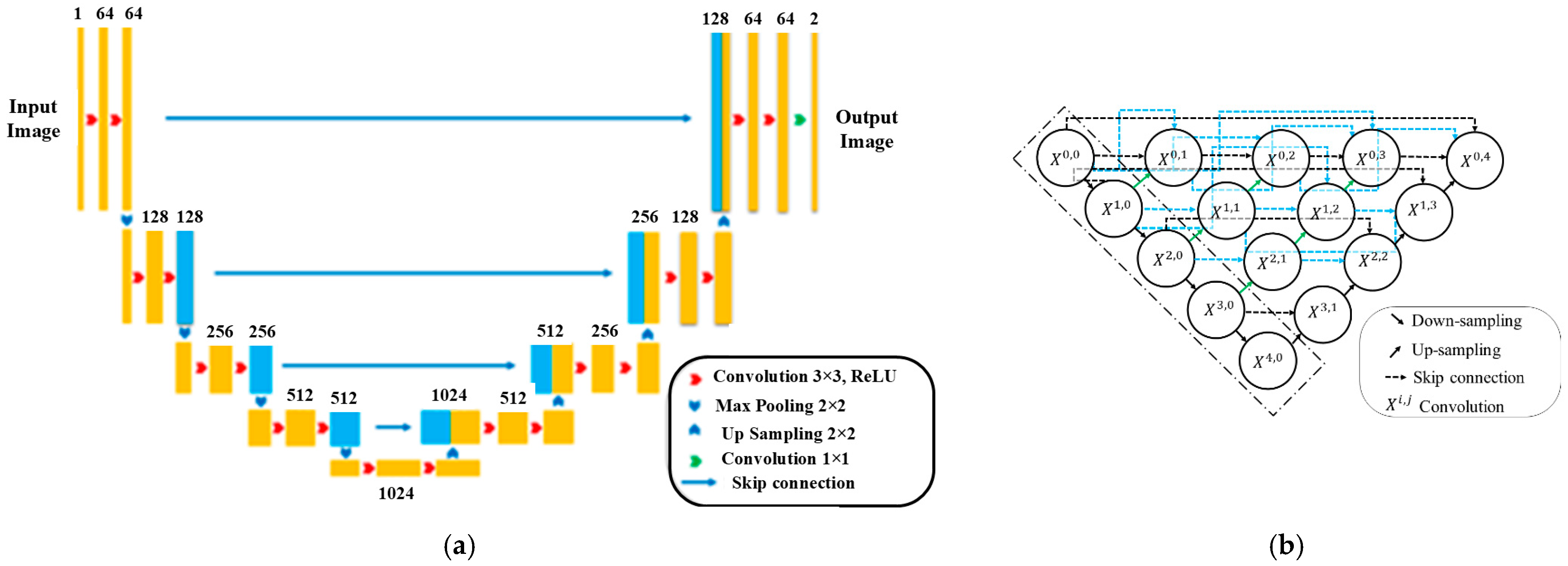
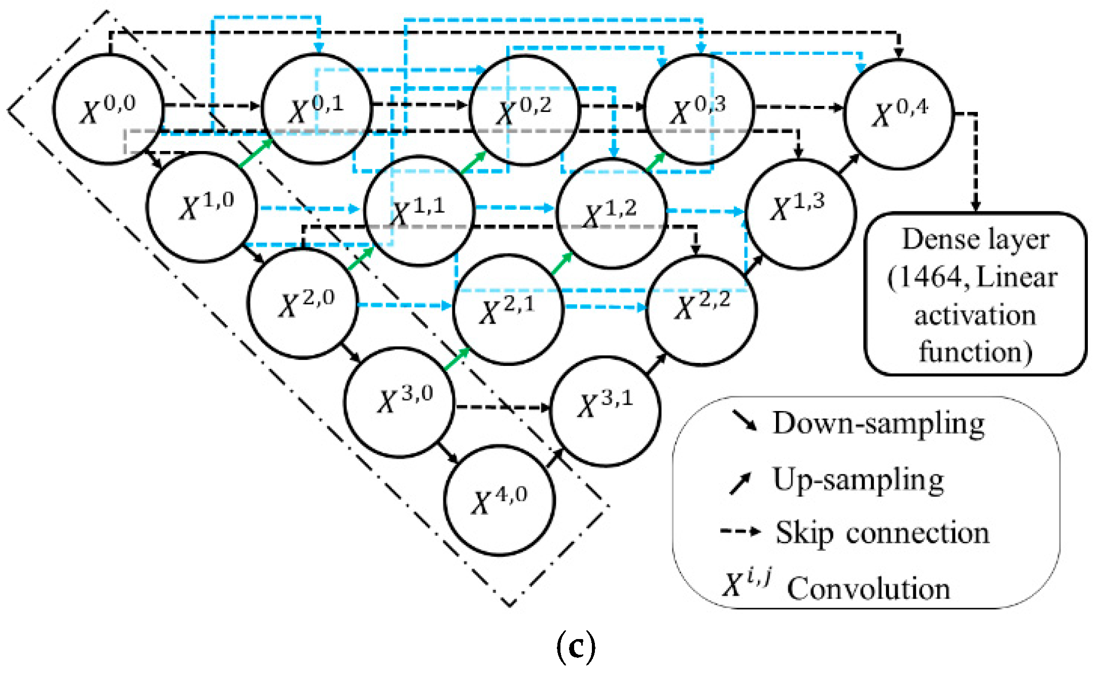
U-Net networks are convolutional structures that encode and decode images. In the encoding stage, the input image dimensions are halved, and channels are doubled using 2D convolutional layers and maxpooling, aiding information extraction. However, identifying which part of the image this information comes from is challenging. U-Net decodes this information by doubling image dimensions and halving channels. The symmetric encoding and decoding process ensures the output size matches the input. To improve gradient flow, the U-Net++ structure redesigns skipping paths between the encoder and decoder networks, incorporating dense connections to enhance encoder outputs and increase modeling accuracy. The current study addresses a regression problem by adding a dense layer to the last layer of U-Net++. The U-Net++ is an advanced structure of convolutional neural networks (CNNs). This algorithm, by using an encoder–decoder and skip connections, extracts the spatial information of the input dataset. However, the CNN may lose the spatial information [31]. Moreover, LSTM-based algorithms are suitable for time series modeling. In the present study, the spatial information of the input dataset is essential, and it is not our aim to discuss time series modeling. Hence, U-Net++ is a good alternative for solving the downscaling problem because of its high performance in extracting spatial information. Figure 2 illustrates the U-Net, U-Net++, and the proposed U-Net++ algorithm for regression problems.

2.10. Gaussian Copula Function

In the Gaussian copula function, the dependence between variables is defined by symmetry and a positive definite matrix whose elements represent the dependence between the combinations of variables. This function is used when the number of variables exceeds two or three. The Gaussian copula function has been used in various hydrological studies such as [32,33]. The following relation defines the Gaussian copula function:

$$c\left(u_1,u_2,\dots ,u_d\right)={\varphi }_d\left({\varphi }^{-1}\left(u_1\right),{\varphi }^{-1}\left(u_2\right),\dots ,{\varphi }^{-1}\left(u_d\right)\right)$$

(6)

In Equation (6), $\phi$ is a normal cumulative distribution function with a mean of zero and a standard deviation of 1. Moreover, ${\phi }_d$ is a multivariate normal distribution function with mean of zero and covariance matrix equal to ∑. The Gaussian copula function is computationally efficient and works well in high-dimensional data.

2.11. Drought Evaluation

This study uses the standardized flow index (SDI) to assess hydrological drought in Iran. This index is a valid measure for assessing hydrological drought and was first introduced to the scientific community by [34]. Using this index, drought phenomena can be assessed using only river flow data and without the need for information such as precipitation and evapotranspiration. The following relationship is used to estimate the SDI:

$$SD{I}_i={\displaystyle \frac{Q_i-\overline{Q}}{Q_{std}}}$$

(7)

where $Q_i$ is the monthly flow rate, $\overline{Q}$ is the average river flow, $Q_{std}$ the standard deviation of the river flow, and i represents the i-th month. Since drought is a creeping phenomenon and usually occurs over a long period; 3-, 6-, 9-, and 12-month moving averages are taken from the SDI data. In this way, additional and noisy information is removed from the SDI results, and drought events are better identified. According to the study by [34], positive SDI values indicate a wet period. In contrast, values between 0 and −1, values between −1 and −1.5, values between −1.5 and −2, and values smaller than −2 correspond to mild drought, moderate drought, severe drought, and very severe drought, respectively.

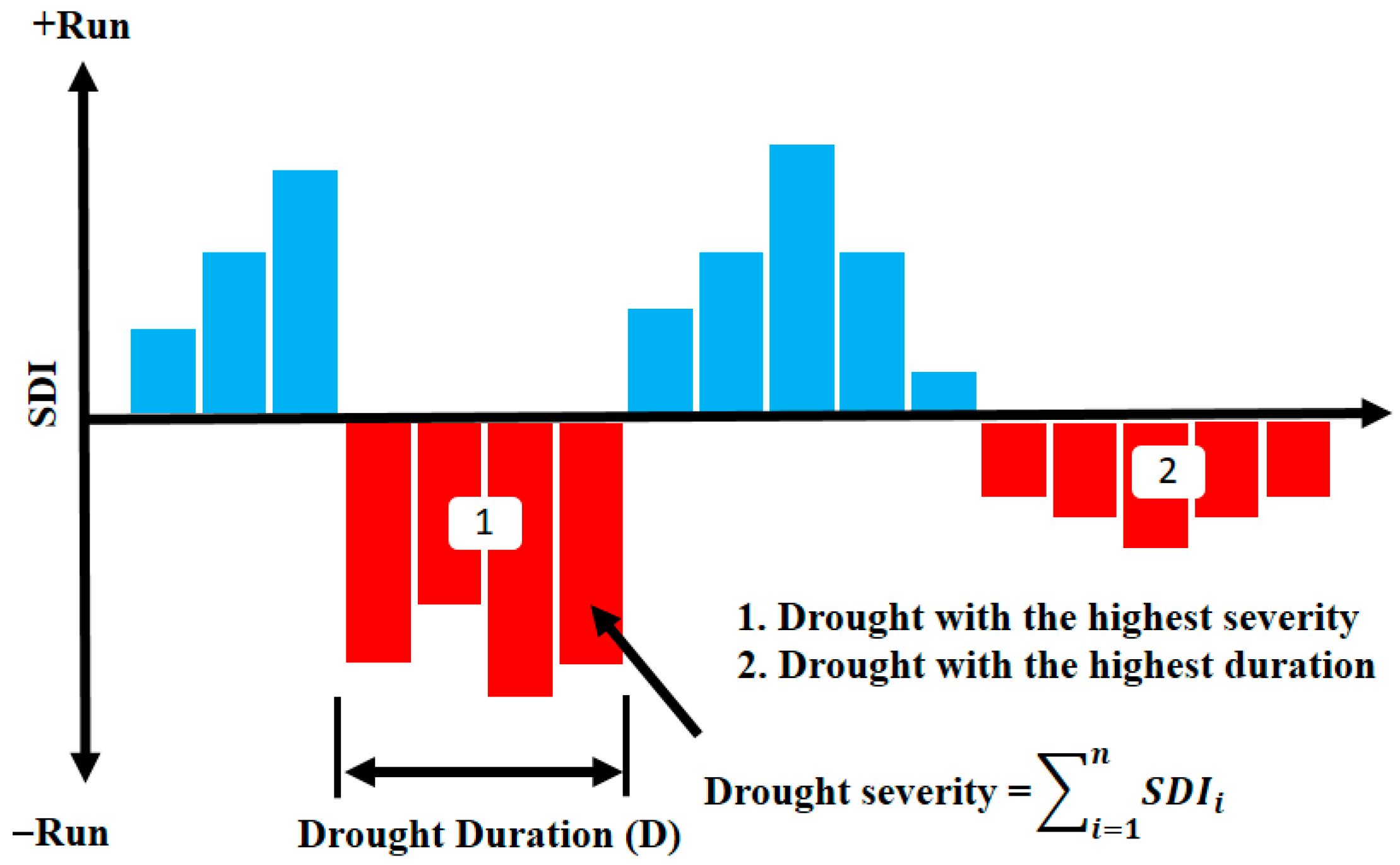
To extract drought events similar to the study by [35], the sequence test is used. This test plots monthly SDI time series data on a graph. Parts of the graph with negative SDI values are drought events, and parts with positive SDI values are wet events. In order to study the drought phenomenon, two measures of severity and duration are examined. Figure 3 shows how the sequence test is used. According to this figure, the severity of a drought is the sum of the negative SDI values for that event. The length of a drought event is its duration.

2.12. Flood Evaluation

The base flow must first be separated from the river flow to extract flood hydrographs. For this purpose, graphical, hydrological, and statistical methods are used. Among them, statistical methods are more popular because of the need for less data. In the statistical method, data with high variations are flood hydrographs, and data with low variations are base flow. 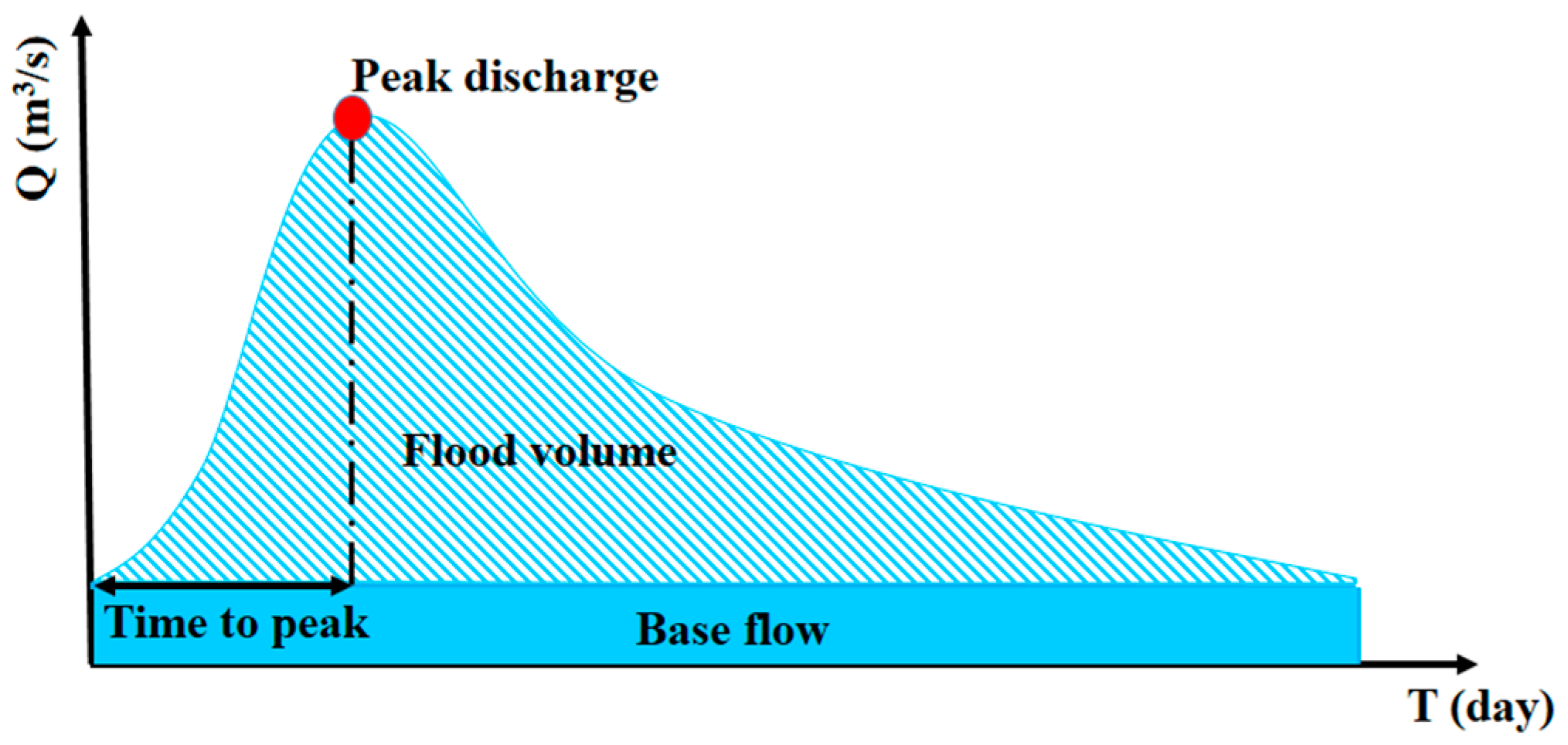One method for statistical separation of base flow was introduced by [36], which has acceptable accuracy. Flood hydrographs are determined after removing the base flow from the daily river flow. Then, the characteristics of the hydrographs, such as maximum discharge values and their occurrence time, can be determined. Figure 4 shows a hydrograph and its characteristics. The hydroEvents software package was used in the present study to perform the above process. For more information about this software package, see [37].

2.13. Downscaling River Flow Data

In this study, drought and flood data for both the base and future periods were extracted from observed and projected river flow data, respectively. For river flow data projection, ISIMIP3b downscaling is used. The river flows in the ISIMIP3b model are large-scale and have a spatial resolution of 0.5 degrees latitude by 0.5 degrees longitude. Therefore, evaluating climate change studies based on these data can be associated with errors. Therefore, in the present study, deep learning is used to downscale river flows in Iran. In the baseline period, deep learning creates a regression relationship between the flow of each hydrometric station and the large-scale ISIMIP3b data, the geographical coordinates of that station, and the flow of that station on the previous day. Then, based on the aforementioned regression relationship, the flow values at each hydrometric station in the future period are predicted for 1464 stations. In this way, the ISIMIP3b network’s flow data can be converted from a scale of 0.5 × 0.5 to flow data at each point in the river. Figure 5 shows the process of downscaling in the present study. As is seen, the bias of U-Net++ outputs is corrected based on the multiple linear regression (MLP), multiple nonlinear regression (MNLR), M5 tree model (M5), multivariate adaptive regression spline (MARS), and quantile mapping (QM).

2.14. Vulnerability Calculation Method

When calculating vulnerability, the criteria of drought severity, drought duration, flood peak flow, and population have a direct relationship with vulnerability. The amount of vulnerability is inversely related to gross domestic product (GDP) and the time interval between drought and flood. Therefore, in this study, the vulnerability relationships are defined as follows:

$$\begin{array}{l}vulnerability\left({\displaystyle \frac{m^3\times year\times millio{n}^2}{s\times billion}}\right)=\\ {\displaystyle \frac{\left|SDI\right|\times Duration\left(month\right)\times Q_{peak}\left(\frac{m^3}{s}\right)\times Pop\left(million\right)}{D\left(month\right)\times GDP\left(\frac{billion}{year \times million}\right)}}\end{array}$$

(8)

In Equation (8), $SD$ is the severity of the drought, $Duration$ is the drought period’s duration, $Q_{peak}$ is the peak flood flow, Pop is the population, $D$ is the time interval between the occurrence of the flood and drought, and $GDP$ is the gross domestic product.

This study examines the interplay between drought and flood exposure, with population linked to vulnerability and resilience reflecting society’s recovery ability. A larger population increases the impact of these disasters, while higher resilience helps mitigate their damage, enhancing overall resilience. Distribution data from Iran in 2016 is utilized as a basis to project the population. The population for baseline and future periods is derived from historical scenario outputs and provincial populations relative to the national total. For future GDP distribution, the 2019 provincial share of national GDP serves as a calculation basis, which, combined with historical outputs, reveals spatial and temporal GDP changes in Iran.

2.15. Evaluation Criteria

In the present research, error evaluation criteria, including mean absolute error (MAE), root mean square error (RMSE), relative root mean square error (RRMSE), Nash–Sutcliffe coefficient criterion (NSE), and percent bias (PBias) have been used. The criteria for MAE, RMSE, RRMSE, NSE, and PBias can be calculated from Equations (9)–(13), respectively [38].

$$MAE={\displaystyle \sum _{i=1}^N\frac{\left|Y_i^{sim}-Y_i^{obs}\right|}{N}}$$

(9)

$$RMSE=\sqrt{{\displaystyle \sum _{i=1}^N\frac{{\left(Y_i^{sim}-Y_i^{obs}\right)}^2}{N}}}$$

(10)

$$RRMSE={\displaystyle \frac{RMSE}{Std}}$$

(11)

$$NSE=1-\left({\displaystyle \frac{{\displaystyle \sum _{i=1}^N{\left(Y_i^{obs}-{\overline{Y}}_i^{sim}\right)}^2}}{{\displaystyle \sum _{i=1}^N{\left(Y_i^{obs}-{\overline{Y}}_i^{obs}\right)}^2}}}\right)$$

(12)

$$PBias={\displaystyle \frac{{\displaystyle \sum _{i=1}^N\left(Y_i^{obs}-Y_i^{sim}\right)}}{{\displaystyle \sum _{i=1}^N{Y}_i^{obs}}}}\times 100$$

(13)

The MAE and RMSE measures range from zero to positive infinity, and their optimal value is zero. This criterion is between 0 and 1, and the closer it is to 1, the higher the simulation accuracy. The PBias measure varies from negative infinity to positive infinity, and its values close to zero indicate less unbiasedness. For PBias, values of less than 10% indicate very good model performance. RRMSE values between 0 and 0.5 are very good. Values greater than 0.7 of this criterion indicate poor simulation performance [39].

3. Results

In this section, first, downscaling of the large-scale ISIMIP3b river flow was performed based on the U-Net++, U-Net++MLR, U-Net++MNLR, U-Net++M5, U-Net++MARS, and U-Net++QM algorithms. In the next step, the flow of Iranian rivers was predicted by considering the best downscaling method and the GFDL-ESM4, MRI-ESM2, and UKESM1-0-II models according to the SSP126, SSP370, and SSP585 scenarios. The fuzzy uncertainty method was used to determine the uncertainty in predicting river flows in Iran. After that, the drought and flood characteristics and vulnerability for the base period as well as near and far future periods are calculated and reported.

3.1. Downscaling River Flow

In this subsection of the present research, downscaling of the country’s river flows has been carried out based on the large-scale ISIMIP3b data and deep learning methods in the basic period. In the following, the accuracy of six integrated deep learning methods in the downscaling of the large-scale GFDL, MRI_ESM2, and UKESM1 data has been investigated. These methods include U-Net++, U-Net++MLR, U-Net++MNLR, U-Net++M5, U-Net++MARS, and U-Net++QM.

The results of the mean, minimum, median, and maximum evaluation criteria obtained from the combined deep learning methods of the training station for estimating river flow at 1464 hydrometric stations of the country based on the large-scale GFDL data are presented in

Table 3. Evaluating the performance of GFDL data downscaling by deep learning models during training.

Algorithm	MAE (m3/s)	RRMSE	PBias	NSE
Mean
U-Net++	7.50	3.30	−0.21	−21.57
U-Net++MLR	5.63	1.09	−0.06	−0.51
U-Net++MNLR	5.64	1.10	−0.06	−0.54
U-Net++M5	5.64	1.14	−0.07	−1.06
U-Net++MARS	5.65	1.12	−0.07	−0.76
U-Net++QM	6.38	1.62	−0.05	−7.16
Min
U-Net++	1.89	0.63	0.00	−339.85
U-Net++MLR	0.07	0.46	0.00	−65.22
U-Net++MNLR	0.07	0.47	0.00	−88.33
U-Net++M5	0.07	0.47	0.00	−417.18
U-Net++MARS	0.07	0.47	0.00	−138.60
U-Net++QM	0.10	0.50	0.00	−1760.64
Median
U-Net++	2.86	1.90	0.31	−2.63
U-Net++MLR	1.32	0.98	0.12	0.03
U-Net++MNLR	1.32	0.98	0.12	0.03
U-Net++M5	1.32	0.99	0.12	0.02
U-Net++MARS	1.33	0.99	0.12	0.01
U-Net++QM	1.40	1.16	0.10	−0.34
Max
U-Net++	271.69	18.46	9.65	0.60
U-Net++MLR	266.10	8.14	6.07	0.78
U-Net++MNLR	264.31	9.45	6.24	0.78
U-Net++M5	269.43	20.45	5.59	0.78
U-Net++MARS	267.26	11.81	5.92	0.78
U-Net++QM	306.78	41.97	4.38	0.75

. According to this table, performing the U-Net++MLR algorithm in the training period is better than the other algorithms studied. This algorithm improved results more than the other five algorithms in 11 out of 16 criteria. Also, the U-Net++QM algorithm competes with other algorithms. This algorithm has better results than the other algorithms in terms of unbiasedness.

In the test period (

Table 4. Evaluating the performance of GFDL data downscaling by deep learning models during testing.

Algorithm	MAE (m3/s)	RRMSE	PBias	NSE
Mean
U-Net++	7.51	6.01	2.87	−82.36
U-Net++MLR	5.60	1.81	4.12	−11.94
U-Net++MNLR	5.59	1.83	4.10	−13.09
U-Net++M5	5.57	1.92	4.10	−18.03
U-Net++MARS	5.57	1.92	4.10	−17.94
U-Net++QM	6.97	2.61	4.18	−17.42
Min
U-Net++	1.80	0.80	0.00	−6797.95
U-Net++MLR	0.07	0.42	0.00	−6194.28
U-Net++MNLR	0.07	0.42	0.00	−6115.57
U-Net++M5	0.07	0.43	0.00	−8196.22
U-Net++MARS	0.07	0.42	0.00	−8323.71
U-Net++QM	0.10	0.58	0.00	−4719.39
Median
U-Net++	2.86	1.90	0.31	−2.63
U-Net++MLR	1.52	1.18	0.40	−0.40
U-Net++MNLR	1.52	1.18	0.40	−0.39
U-Net++M5	1.52	1.21	0.39	−0.48
U-Net++MARS	1.52	1.22	0.39	−0.49
U-Net++QM	1.64	1.74	0.43	−2.01
Max
U-Net++	271.14	82.44	750.73	0.36
U-Net++MLR	241.74	78.70	562.88	0.83
U-Net++MNLR	240.44	78.20	562.28	0.82
U-Net++M5	242.26	90.52	558.31	0.82
U-Net++MARS	246.70	91.23	556.21	0.82
U-Net++QM	394.21	68.69	569.61	0.66

), U-Net++QM had competitive results with other algorithms. This algorithm had good results on most of the criteria. Based on the maximum results, the RRMSE value for this algorithm is approximately 17%, 13%, 12%, 24%, and 25% lower than the algorithms U-Net++, U-Net++MLR, U-Net++M5, and U-Net++MARS, respectively.

The mean, minimum, median, and maximum of the MAE, RRMSE, PBias, and NSE evaluation criteria during the training period for downscaling the MRI model river flow at 1464 hydrometric stations are presented in Table 4 and

Table 5. Evaluating the performance of MRI data downscaling by deep learning models during training.

Algorithm	MAE (m3/s)	RRMSE	PBias	NSE
Mean
U-Net++	6.83	3.38	−0.16	−24.02
U-Net++MLR	5.89	1.10	−0.06	−0.52
U-Net++MNLR	5.91	1.10	−0.06	−0.53
U-Net++++M5	5.86	1.15	−0.07	−0.88
U-Net++MARS	5.85	1.14	−0.07	−0.78
U-Net++QM	5.66	1.63	−0.01	−9.57
Min
U-Net ++	1.84	0.58	0.00	−278.56
U-Net ++MLR	0.07	0.47	0.00	−56.95
U-Net ++MNLR	0.07	0.47	0.00	−68.37
U-Net ++M5	0.07	0.49	0.00	−145.13
U-Net ++MARS	0.07	0.48	0.00	−123.34
U-Net ++QM	0.10	0.49	0.00	−2982.15
Median
U-Net ++	2.78	1.91	0.26	−2.64
U-Net ++MLR	1.32	0.99	0.11	0.02
U-Net ++MNLR	1.33	0.99	0.12	0.02
U-Net ++M5	1.32	1.00	0.12	0.00
U-Net ++MARS	1.33	1.00	0.12	−0.01
U-Net ++QM	1.39	1.14	0.08	−0.31
Max
U-Net ++	245.18	16.72	9.06	0.66
U-Net ++MLR	279.54	7.61	5.45	0.78
U-Net ++MNLR	285.84	8.33	5.61	0.78
U-Net ++M5	287.64	12.09	5.82	0.76
U-Net ++MARS	280.67	11.15	5.65	0.77
U-Net ++QM	255.35	54.61	6.09	0.76

. Based on the results of this table, U-Net++MLR outperformed the other algorithms in 12 out of 16 criteria. The results of U-Net++QM were also comparable to the other algorithms.

In the test period, the results of the minimum, average, median, and maximum evaluation criteria for the MRI model are given in

Table 6. Evaluating the performance of MRI data downscaling by deep learning models during testing.

Algorithm	MAE (m3/s)	RRMSE	PBias	NSE
Mean
U-Net++	6.76	5.74	3.19	−72.89
U-Net++MLR	5.79	1.94	4.12	−19.96
U-Net++MNLR	5.77	1.98	4.12	−23.45
U-Net ++M5	5.69	2.10	4.08	−30.75
U-Net++MARS	5.70	2.13	4.09	−32.14
U-Net++QM	6.16	2.41	3.89	−14.33
Min
U-Net ++	1.82	0.81	0.00	−4553.61
U-Net++MLR	0.07	0.44	0.00	−10,792.16
U-Net++MNLR	0.07	0.42	0.00	−15,260.35
U-Net++M5	0.07	0.46	0.00	−20,864.48
U-Net++MARS	0.07	0.43	0.00	−21,860.62
U-Net++QM	0.09	0.55	0.00	−3894.45
Median
U-Net++	2.82	2.58	0.40	−5.68
U-Net++MLR	1.54	1.20	0.40	−0.44
U-Net++MNLR	1.54	1.21	0.40	−0.46
U-Net++M5	1.51	1.23	0.40	−0.52
U-Net++MARS	1.52	1.24	0.40	−0.55
U-Net++QM	1.59	1.57	0.33	−1.47
Max
U-Net++	218.73	67.48	526.64	0.35
U-Net++MLR	256.95	103.87	560.36	0.81
U-Net++MNLR	253.85	123.52	561.44	0.82
U-Net++M5	253.55	144.43	548.15	0.79
U-Net++MARS	255.58	147.83	558.11	0.81
U-Net++QM	363.75	62.40	564.08	0.70

. According to the results of this table, the U-Net++QM algorithm achieved competitive results compared to the other five algorithms. The maximum RRMSE criterion values for this algorithm were approximately 8%, 40%, 49%, 57%, and 58% lower compared to U-Net++, U-Net++MLR, U-Net++MNLR, U-Net++M5, and U-Net++MARS, respectively.

The results of the mean, minimum, median, and maximum of the training period’s evaluation criteria for estimating river flow at 1464 hydrometric stations in the country based on the large-scale UKESM1 data can be seen in

Table 7. Evaluating the performance of UKESM1 data downscaling by deep learning models during training.

Algorithm	MAE (m3/s)	RRMSE	PBias	NSE
Mean
U-Net++	7.56	3.38	−0.18	−23.75
U-Net++MLR	5.62	1.09	−0.06	−0.52
U-Net++MNLR	5.65	1.10	−0.06	−0.56
U-Net++M5	5.68	1.16	−0.07	−1.21
U-Net++MARS	5.68	1.15	−0.06	−1.02
U-Net++QM	6.42	1.60	−0.04	−7.60
Min
U-Net++	2.01	0.76	0.00	−311.79
U-Net++MLR	0.07	0.47	0.00	−80.66
U-Net++MNLR	0.07	0.47	0.00	−107.63
U-Net++M5	0.07	0.48	0.00	−232.88
U-Net++MARS	0.07	0.47	0.00	−260.48
U-Net++QM	0.10	0.52	0.00	−2639.80
Median
U-Net++	2.78	1.94	0.23	−2.75
U-Net++MLR	1.32	0.98	0.12	0.04
U-Net++MNLR	1.32	0.98	0.12	0.03
U-Net++M5	1.32	0.99	0.12	0.02
U-Net++MARS	1.33	0.99	0.12	0.01
U-Net++QM	1.40	1.15	0.09	−0.32
Max
U-Net++	272.05	17.68	8.19	0.42
U-Net++MLR	262.43	9.04	6.33	0.78
U-Net++MNLR	263.53	10.42	6.22	0.78
U-Net++M5	267.67	15.29	5.58	0.77
U-Net++MARS	265.91	16.17	6.29	0.78
U-Net++QM	314.09	51.39	5.96	0.72

. According to this table, the U-Net++MLR algorithm outperforms the other algorithms studied in the training period. This algorithm outperforms the other five algorithms on 11 out of 16 criteria. The performance of the U-Net++QM algorithm was also comparable to this algorithm.

In the test period (

Table 8. Evaluating the performance of UKESM1 data downscaling by deep learning models during testing.

Algorithm	MAE (m3/s)	RRMSE	PBias	NSE
Mean
U-Net++	7.34	6.29	3.92	−91.34
U-Net++MLR	5.57	1.80	4.11	−11.28
U-Net ++MNLR	5.57	1.82	4.10	−11.92
U-Net ++M5	5.57	1.92	4.09	−15.99
U-Net ++MARS	5.57	1.95	4.09	−17.37
U-Net ++QM	6.41	2.65	4.33	−22.75
Min
U-Net ++	1.88	0.77	0.00	−7092.54
U-Net ++MLR	0.07	0.42	0.00	−4897.82
U-Net ++MNLR	0.07	0.43	0.00	−4328.46
U-Net ++M5	0.07	0.43	0.00	−6398.26
U-Net ++MARS	0.07	0.43	0.00	−7501.15
U-Net ++QM	0.09	0.57	0.00	−8117.01
Median
U-Net ++	3.09	2.86	0.50	−7.19
U-Net ++MLR	1.52	1.17	0.40	−0.38
U-Net ++MNLR	1.52	1.18	0.39	−0.38
U-Net ++M5	1.52	1.21	0.39	−0.46
U-Net ++MARS	1.53	1.22	0.40	−0.48
U-Net ++QM	1.67	1.70	0.37	−1.87
Max
U-Net ++	210.65	84.21	657.25	0.40
U-Net ++MLR	242.14	69.98	561.42	0.82
U-Net ++MNLR	240.65	65.79	559.29	0.81
U-Net ++M5	243.38	79.98	557.47	0.82
U-Net ++MARS	245.54	86.60	552.17	0.82
U-Net ++QM	340.71	90.09	531.60	0.68

), U-Net++MLR was superior to the other algorithms in terms of lower error and higher accuracy in 8 out of 16 criteria. However, the U-Net++QM algorithm had close results to this algorithm. The unbiased coefficient values for the maximum results obtained by U-Net++QM were approximately 19%, 5%, 5%, 5%, and 4% lower than the other algorithms.

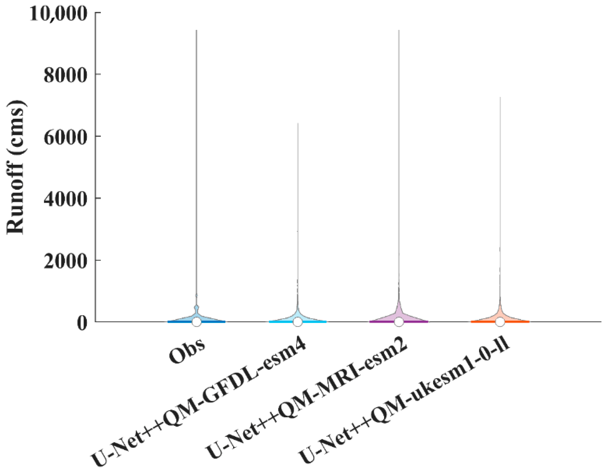
Figure 6 shows the violin plot of the total downscaling outputs of the country’s rivers for the best algorithms for the GFDL, MRI, and UKESM1 models. The violin plot shows the distribution of the modeled data versus the observed data. As seen, the U-Net++QM algorithm models the distribution of the observed data with reasonable accuracy. In addition to the mean values, the maximum values are also estimated with reasonable accuracy by this algorithm. In the meantime, more accuracy has been achieved for the MRI model. Given the acceptable accuracy of U-Net++QM in estimating the maximum and mean values, this algorithm is used to make predictions. QM corrects the distribution of downscaled river flow based on the distribution of the observed data. Machine learning algorithms can be sensitive to bias in input data. Considering the bias in downscaled results of the standalone U-Net++ model, QM corrects this bias by using the distribution of the observed dataset. Hence, QM when using this approach can improve the accuracy of U-Net++.

3.2. Projection the Flow in the Country’s Rivers in the Future

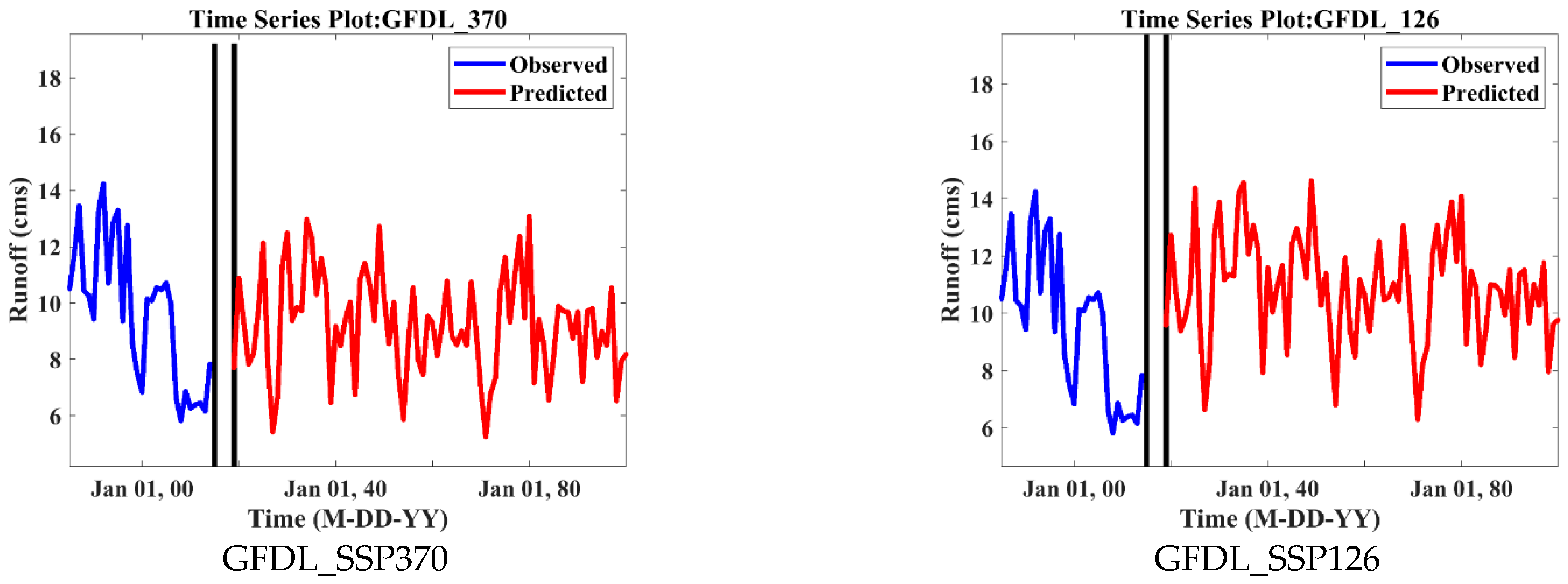
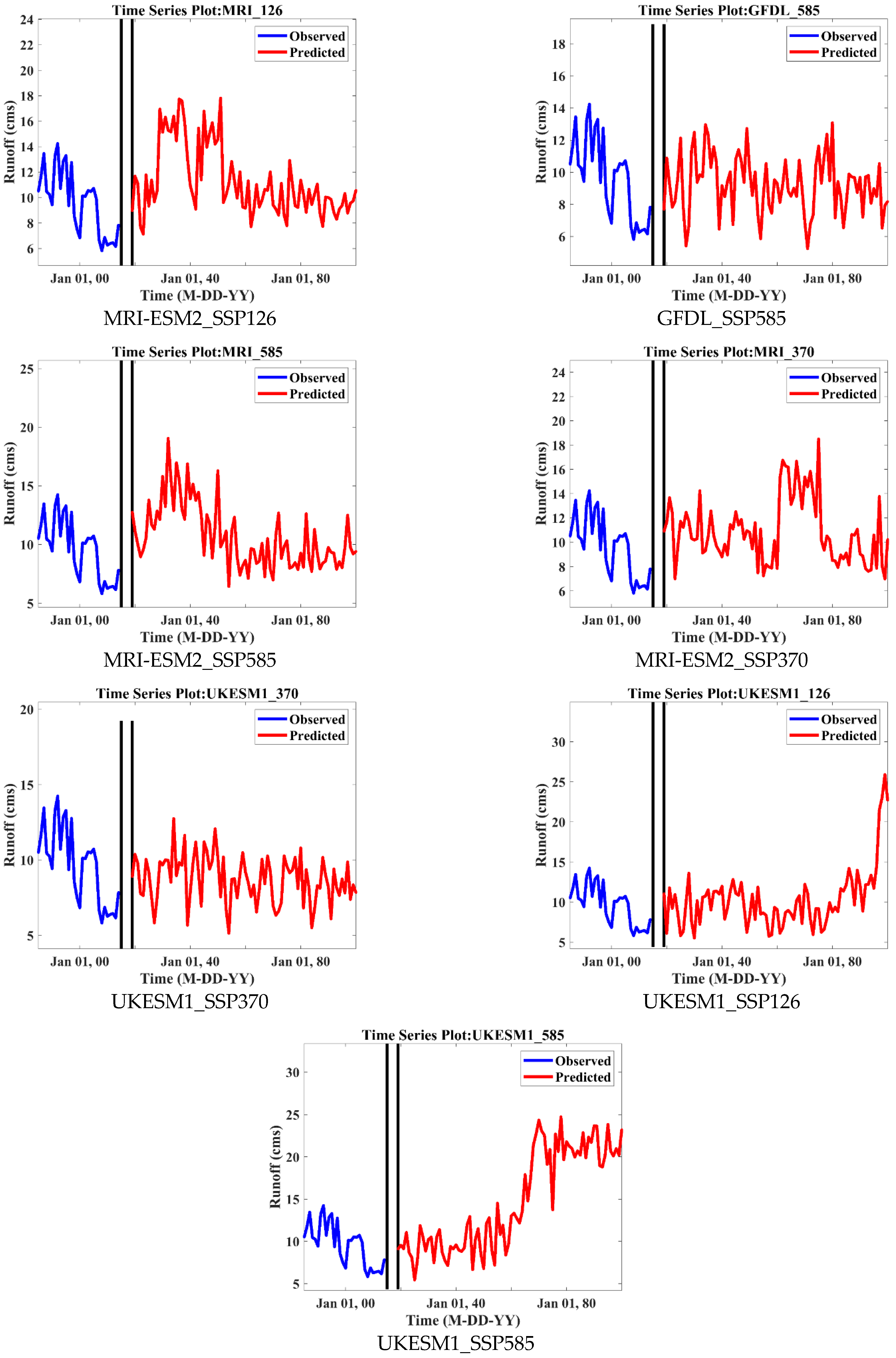
Figure 7 shows the average time series changes in the country’s hydrometric stations for the base period and the future horizon. Based on the forecasts, the amount of river flow at the beginning of the future period (2019) increases compared to the end of the base period (2014). Based on the forecasts made by the GFDL model, the average runoff of the country’s stations has a decreasing trend. With the MRI-ESM2 model, the average runoff time series trend initially increases and then decreases in the future period. The results of runoff forecasting using the UKESM1 model in the SSP126 scenario indicate a decreasing trend in runoff and then an increasing trend in the average runoff time series. With the SSP370 scenario in this model, the amount of runoff has a decreasing trend. However, with the SSP585 scenario in the aforementioned model, sudden changes in the average runoff are predicted after 2060. By observing Figure 7, the evidence shows that the runoff changes in the SSP585 scenario, which is a pessimistic scenario, are more significant than those in the other two scenarios. The observed variation in river flow in this Figure lead to the development of drought and floods in future periods. Moreover, changes in river flow, droughts, and floods can alter the combined impact of floods and droughts. This investigation will be conducted in the following subsections.

3.3. Uncertainty Analysis in River Flow Forecasting in the Future Period (2019–2100)

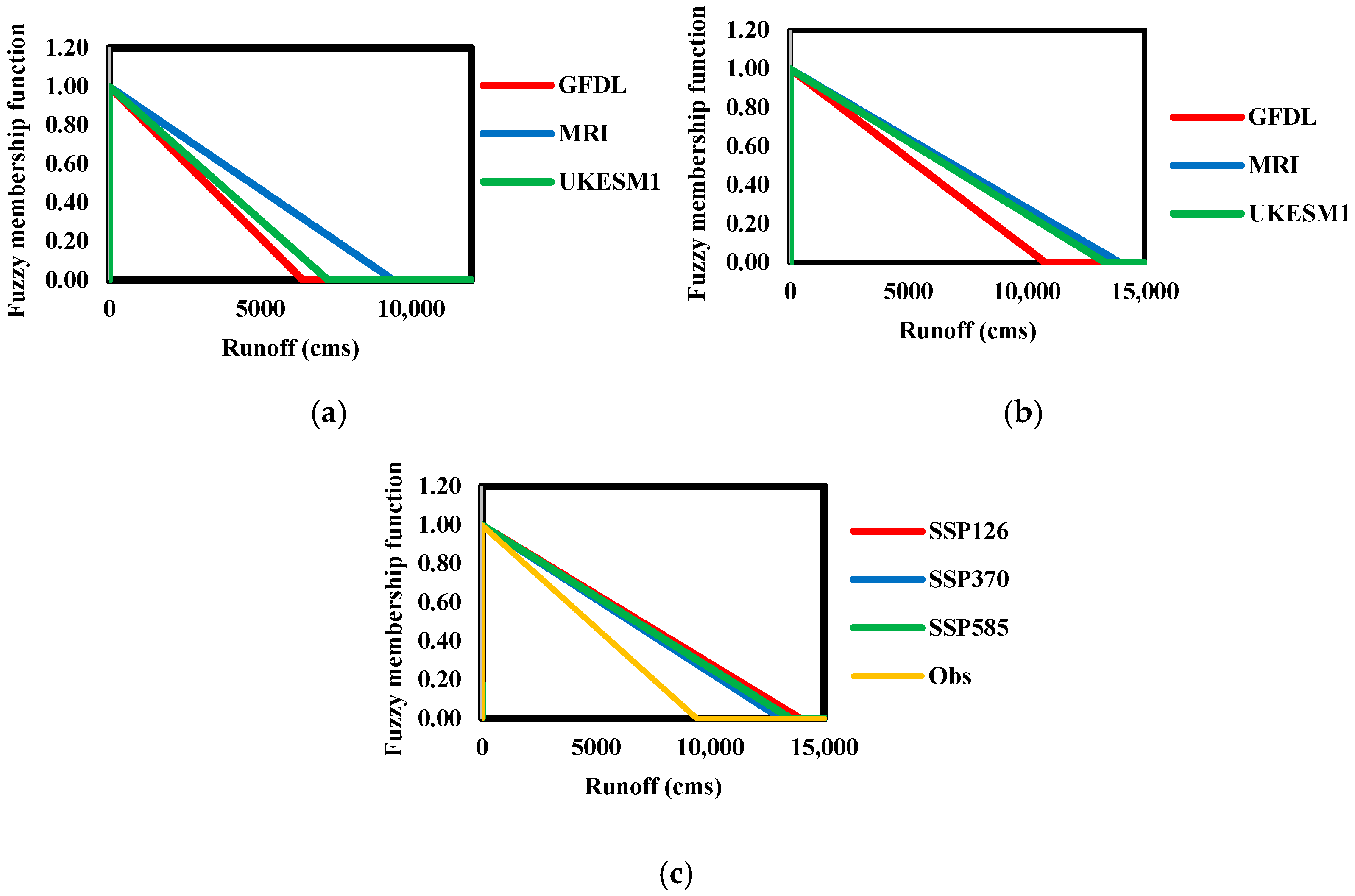
In Figure 8, the results of fuzzy uncertainty analysis for the general circulation models in the base and future periods, and also the climate change scenarios against the base period, can be seen. In the fuzzy uncertainty analysis method, the extreme values, i.e., the maximum and minimum values, are considered with a membership function of zero. The value of the median membership function is also considered equal to one. In this way, a triangle is formed for the three minimum, median, and maximum values. The sharper the triangle, the lower the uncertainty, and the wider the base of the triangle, the greater the uncertainty. Therefore, as seen in Figure 8, the GFDL model has the lowest uncertainty in both the base and future periods, and the UKESM1 model has the highest uncertainty. With climate change scenarios, the highest uncertainty is related to SSP585, and the lowest is related to SSP370. Also, in the base period, the uncertainty of the results is less than in the future period. Therefore, the GFDL model predictions under the SSP370 scenario are more reliable than other general circulation models and climate change scenarios. This could be because of the assumptions made by these models and scenarios.

3.4. Ensemble Model Under SSP126 for 2021–2050

The results of drought intensity, duration, peak flood flow, drought–flood intervals, and their return periods are summarized in the following sections. Figure S1 shows the maximum drought intensity projected from 2021 to 2050 by the deep learning model, indicating that the most severe droughts are expected late in this period, particularly from 2044 to 2047, with a maximum intensity of −80. Figure S2 indicates that drought intensities for SDI1, SDI3, SDI6, and SDI9 range from −5 to −750, with peak values mainly in the northwestern regions. The central areas and the coasts of the Sea of Oman and the Persian Gulf are predicted to have a lower intensity.

Figure S2 shows the drought duration using the Ensemble General Circulation Model (GCM) and SSP126 scenario from 2021 to 2050, predicting significant extensions towards the end, especially from 2044 to 2047, totaling approximately 70 months. Figure S3 displays changes in drought duration for SDI1, SDI3, SDI6, SDI9, and SDI12, ranging from 1 to 40 months, with the longest drought predicted in the east and the shortest in central regions, the coasts of the Sea of Oman, and the western borders. Figure 9 presents the maximum peak flood flow predicted by a deep learning model, exceeding 7000 m³/s, with severe flooding expected in most years during this period. Figure S4 shows flood peak variations, with maximum values for SDI1, SDI3, SDI6, SDI9, and SDI12 ranging from 0 to 400 m³/s, and highlights that the southwestern and northeastern regions will face the highest flood flows. Figure S5 illustrates the maximum interval between droughts and floods, estimated at six months, with drought periods peaking towards the end of the prediction. Figure S6 depicts time intervals between floods and droughts, varying from 1 to 5 months, with the highest in the northwest and the lowest in central regions. 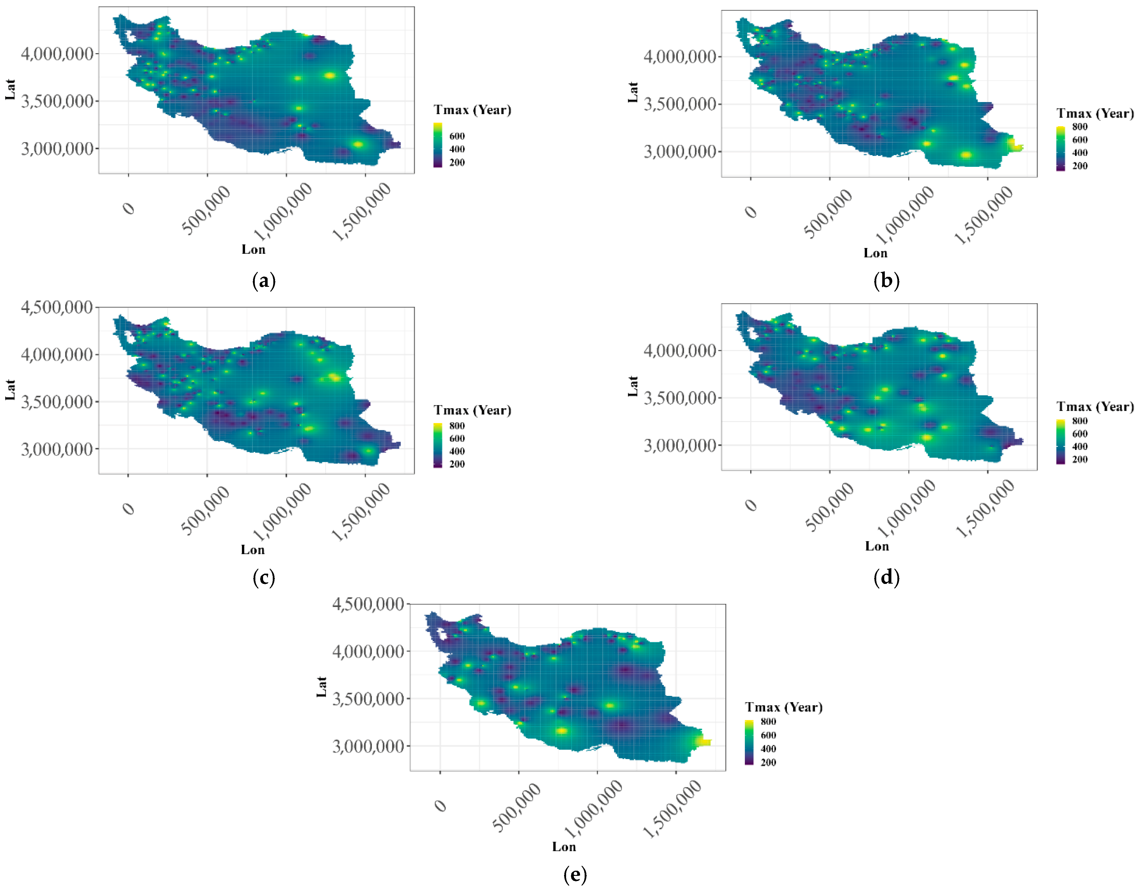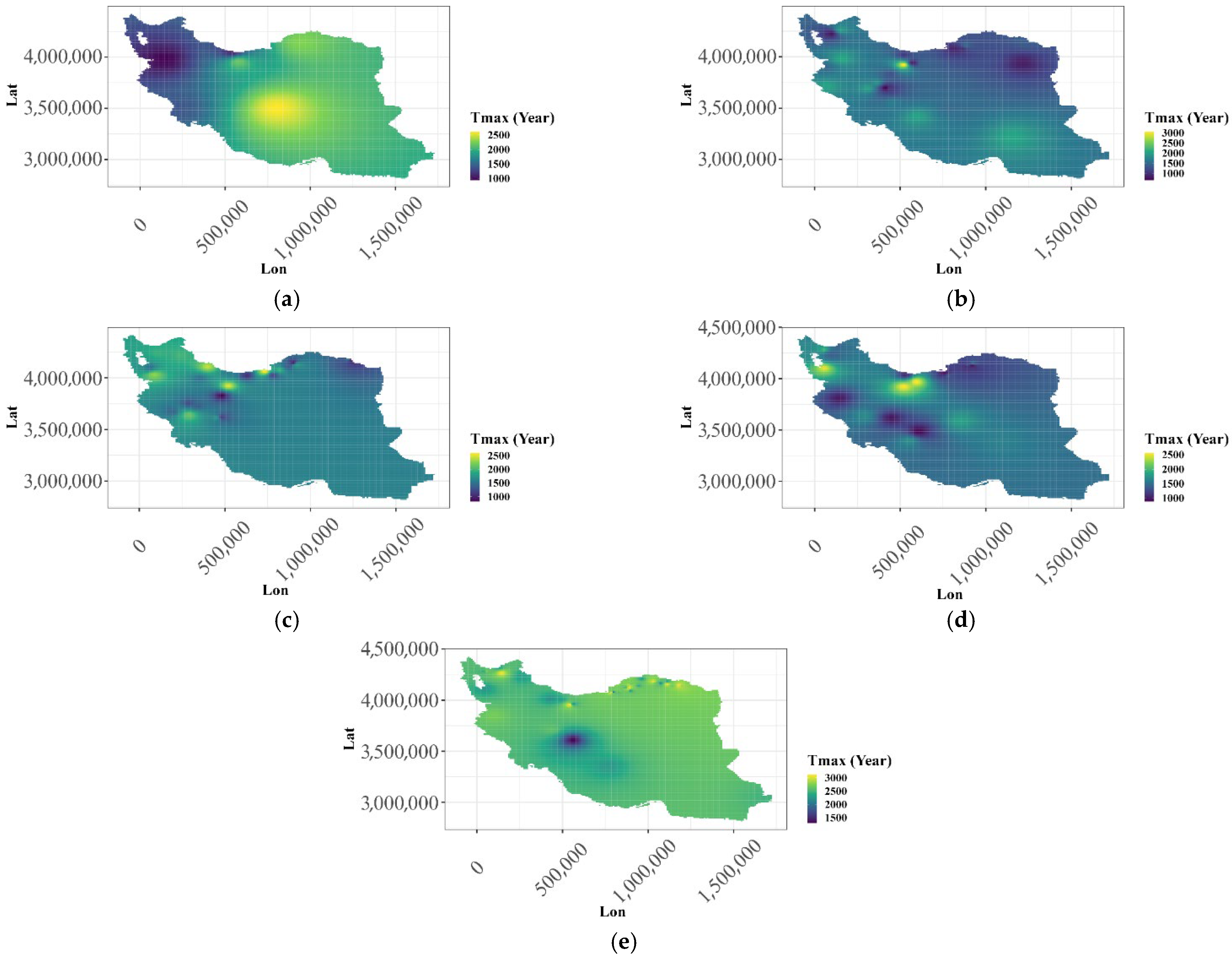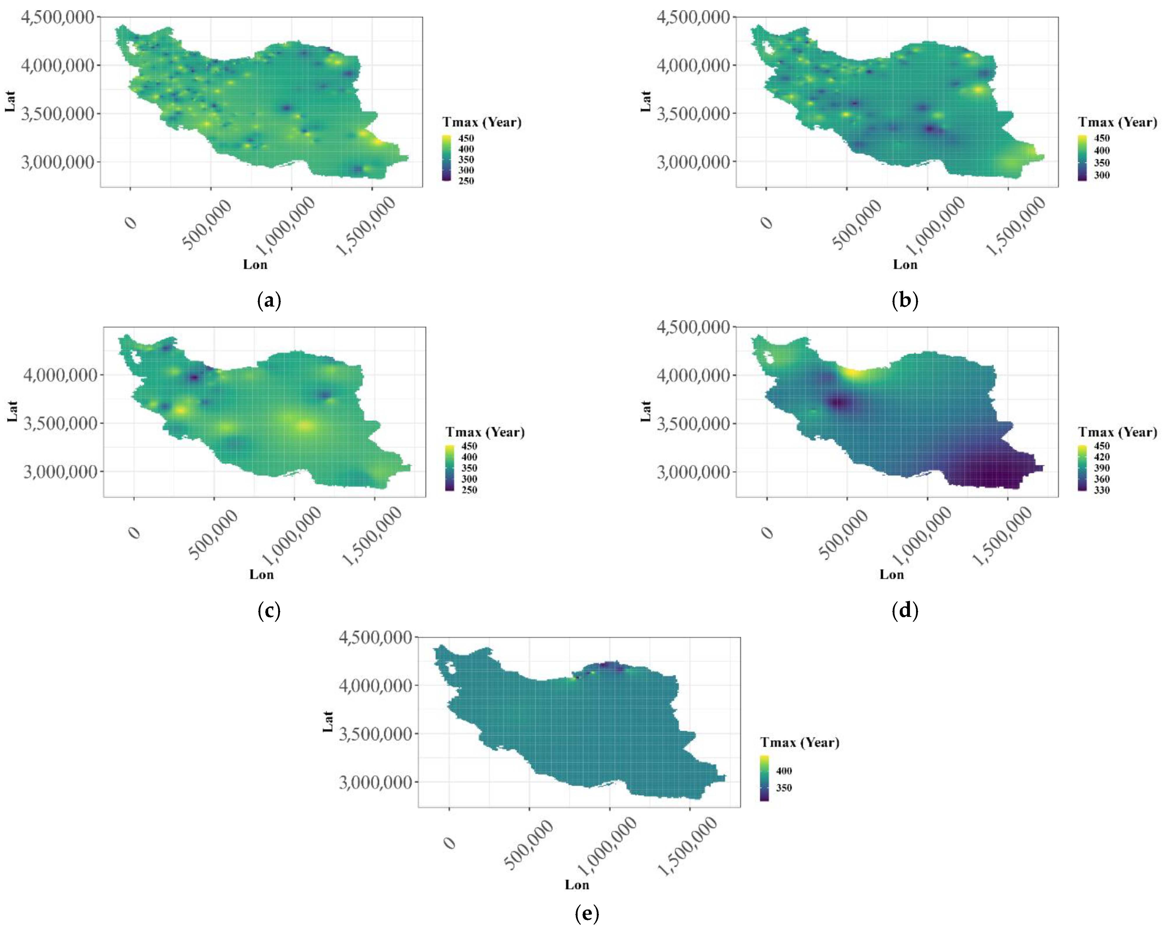Figure 9 illustrates the maximum return period for combined drought and flood, ranging from about 200 to 800 years, with higher values concentrated in southern and eastern regions, while lower values are in central and western areas.

3.5. Ensemble Model Under SSP370 for 2021–2050

The results of the combined projection of droughts and floods, along with their multivariate frequency analysis based on fine-scale river flow using the Ensemble GCM under scenario SSP370, are evaluated below. Figure S7 shows the maximum drought severity predicted by the deep learning model for the near future (2021–2050) and the Ensemble model under the SSP370 scenario. The most severe droughts are forecasted for 2021, 2024–2025, 2044–2045, and 2049, with a maximum predicted severity of −60. Figure S8 demonstrates the maximum drought duration predicted by a deep learning model based on the UKESM1 model and scenario SSP585 for the distant future (2071–2100). Drought durations peak earlier, particularly in 2071 and 2075–2076, with a maximum duration of approximately 350 months, 218% longer than in the near future. Figure S9 shows the projected maximum peak flood flow exceeding 12,000 m³/s, similar to near-future predictions. Severe flooding is expected most years throughout this period. Figure S10 illustrates spatial variations in the maximum flood peak post-drought. Predicted peak values for SDI1, SDI3, SDI6, SDI9, and SDI12 range from 10 to 30 m³/s, 10 to 60 m³/s, 5 to 20 m³/s, 3 to 9 m³/s, and 5 to 8 m³/s, respectively, with the western regions experiencing the highest and eastern the lowest flows. Figure S11 presents the maximum interval between droughts and floods, predicted at 12 months, reflecting an 83% reduction from the near future. Drought duration peaks towards the end of the distant future. Figure S12 shows the time intervals between floods and droughts, ranging from one to five months, with northern regions exhibiting the highest values and central regions the lowest. Figure 10 indicates the maximum return period of the combined drought and flood phenomenon, ranging from approximately 3000 to 1000 years, with northern areas showing the highest and southern and eastern the lowest values.

3.6. Ensemble Model Under SSP585 for 2021–2050

The drought and flood forecasts, including multivariate frequency analysis of downscaled river flows from the Ensemble GCM under the SSP585 scenario, are evaluated. Figure S13 shows the maximum drought severity predicted by the deep learning model for 2021–2050, with severe droughts expected in 2021–2025, 2030–2035, and 2047–2049, reaching a maximum severity of −60. Figure S14 presents maximum drought intensity, which ranges from −6 to −750, peaking in the northern and western regions and being the lowest in the south and southeast. Figure S15 depicts maximum drought duration using the UKESM1 model, showing longer durations in 2021–2025, 2030–2035, and 2047–2049, with a maximum of approximately 55 months. Figure S16 highlights drought period changes for SDI1, SDI3, SDI6, SDI9, and SDI12 as 10–40, 2–8, 20–60, 10–40, and 100–300 months, respectively, with the longest durations in the north and shortest in the southern, eastern, and southwestern regions. Figure S17 illustrates maximum flood peak flows from the deep learning model, with expected peaks exceeding 5000 m³/s during extreme events in 2021–2023, 2026–2034, 2035, 2038, 2040, and 2046–2050. Figure S18 presents maximum flood peak values for SDI1, SDI3, SDI6, SDI9, and SDI12, ranging from 4.8 to 12.5 m³/s, with the highest peaks in the west and south and the lowest in the northeast. Figure S19 shows the maximum interval between droughts and floods, exceeding 22 months and being significant from 2041 to 2050. Figure S20 illustrates time intervals between events, ranging from 1 to 4 months; they are highest in the north and lowest in the south and east. 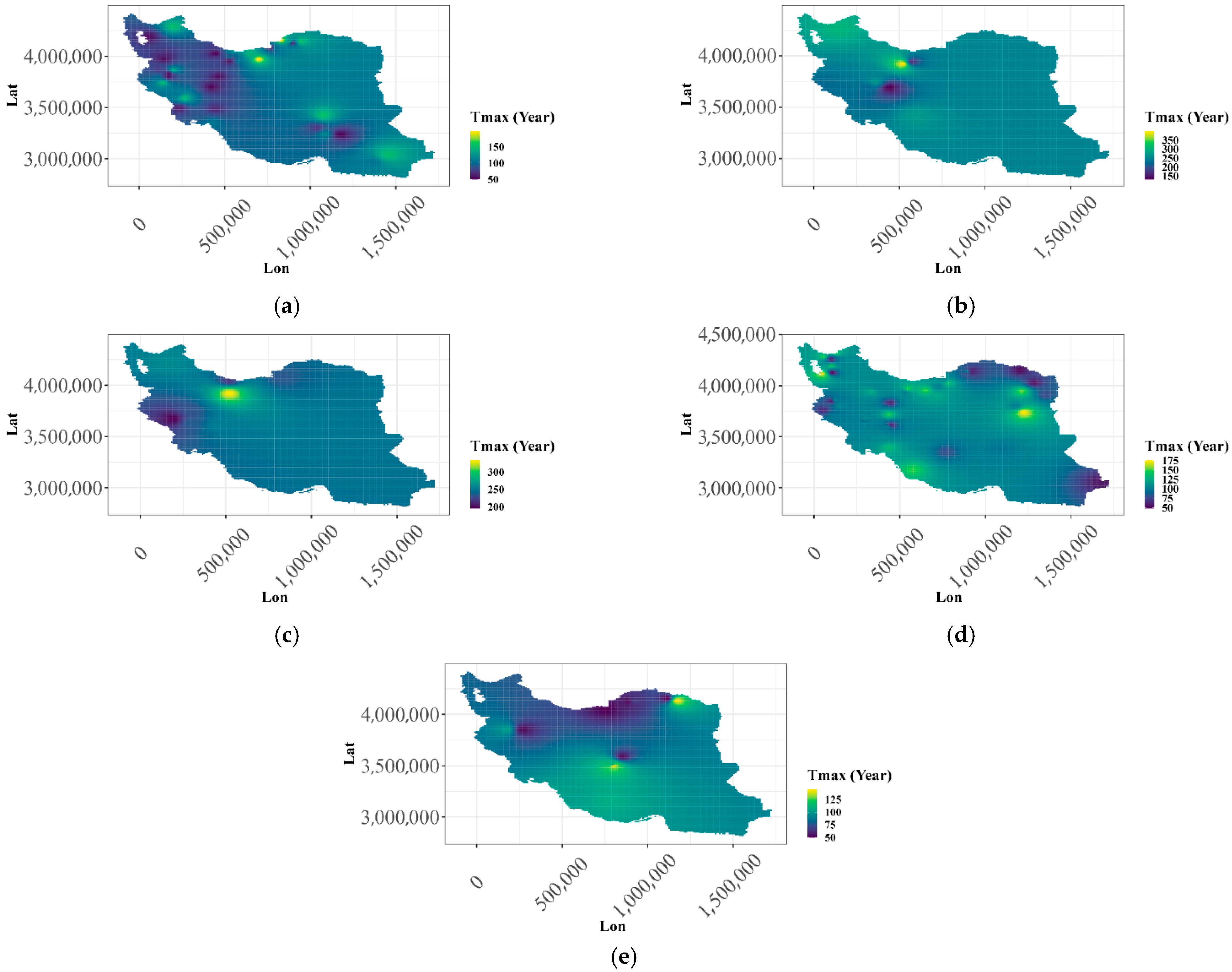Finally, Figure 11 details the maximum return period for combined drought and flood phenomena, with a maximum of approximately 350 years and a minimum of approximately 50 years; it is highest in the north and lowest in the southeast.

3.7. Ensemble Model Under SSP126 for 2071–2100

This analysis examines drought and flood characteristics, focusing on intensity, duration, intervals, and return periods. Figure S26 presents the maximum drought intensity for 2071–2100 predicted by the deep learning model, showing the most severe droughts at the period’s start and end, with intensity peaking around −220, 175% above earlier estimates. Figure S27 illustrates spatial drought intensity from −200 to −800, highest in the northern, eastern, and western regions, and lowest in central and southern areas. Figure S28 depicts the maximum drought duration predicted for 2071–2100, with distant-future droughts lasting over 200 months, 186% longer than near-future droughts. Figure S29 displays drought durations for SDIs 1, 3, 6, 9, and 12 over 1 to 300 months, with the longest durations in the northwest and southeast, and the shortest in the south. Figure S30 forecasts a maximum peak flood flow exceeding 3000 m³/s for 2071–2100, indicating potential severe flooding. Figure S31 predicts drought–flood intervals under scenario SSP585 for 2071–2100, with maximum intervals of 6 months, and longer future drought durations. Figure S32 shows that intervals between events range from 1 to 4 months and are the highest in eastern and western areas, and the lowest in coastal regions. 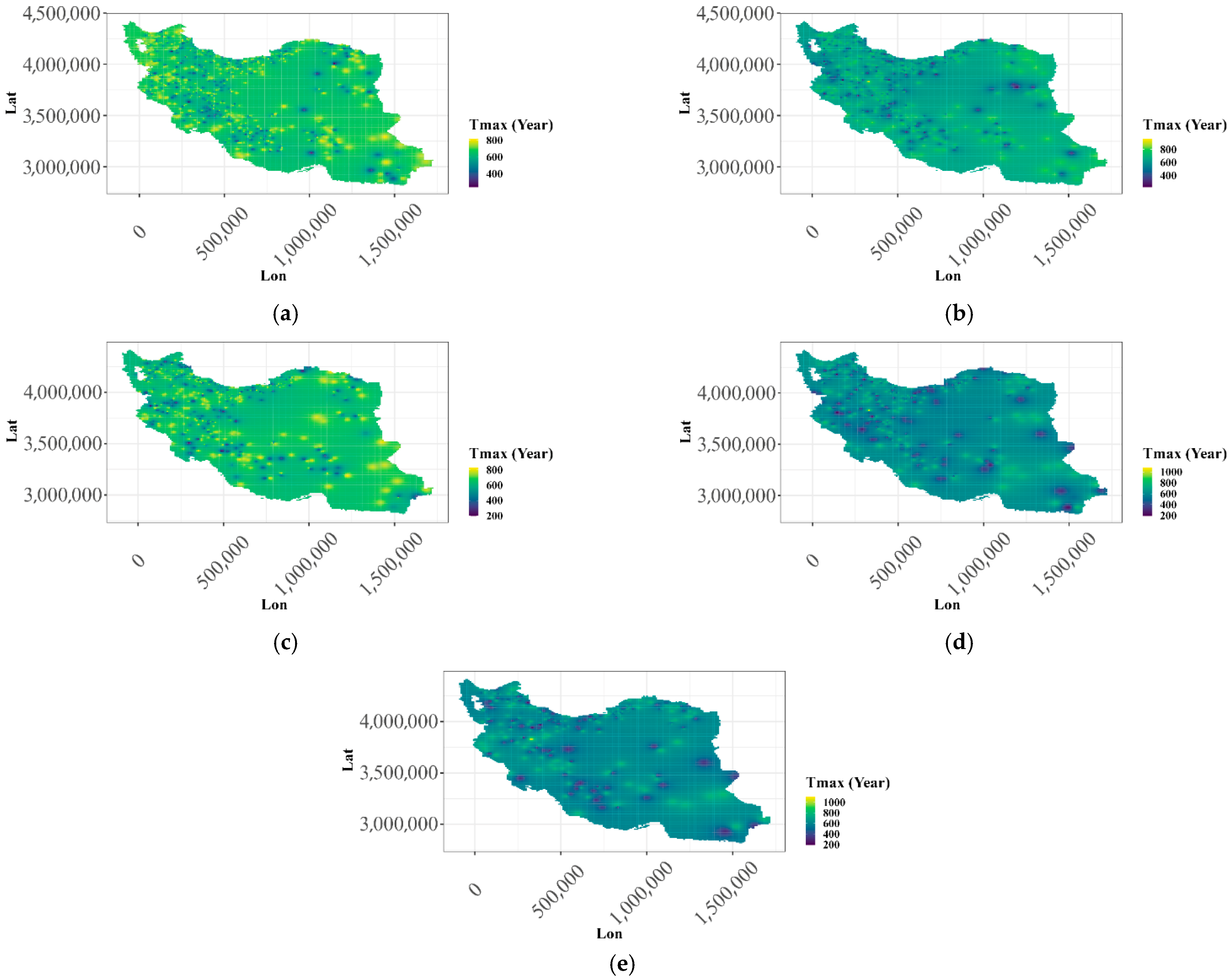Finally, Figure 12 depicts return periods for drought and flood phenomena, reaching approximately 1000 years maximum and 200 years minimum, with the longest periods in the eastern and western regions, and shorter periods in the southern and central areas.

3.8. Ensemble Model Under SSP370 for 2071–2100

This section evaluates combined drought and flood forecasts and multivariate frequency analysis of downscaled river flow using the Ensemble GCM aligned with the SSP370 scenario. Figure S33 shows the maximum drought predicted by a deep learning model for 2071–2100, highlighting severe droughts expected in 2071–2072 and 2087–2088, with a maximum severity of −300. Drought intensity varies spatially from −200 to −750 and is highest in the southwest and west and lowest in the southeast and coastal areas. Figure S34 projects the maximum drought duration using deep learning for 2071–2100, with periods extending longer in the early years, especially 2071–2072. The maximum duration could reach 300 months, a 400% increase from near-future values. Figure S35 illustrates drought variations from 1 to 30 months, which are the longest in the north, west, and east, with shorter durations in the south. Figure S36 shows projected peak flood flows over 3000 m³/s from deep learning using the Ensemble GCM for 2071–2100. Floods of around 3000 m³/s may occur annually, a 40% decrease from near-future levels. Figure S37 illustrates peak flood variations post-drought, with SDI1, SDI3, SDI6, SDI9, and SDI12 flows projected between 0 and 500 m³/s, highest in the northwestern and northeastern regions. Figure S38 predicts a maximum time interval between droughts and floods at 6 months for 2071–2100, similar to the near future. Figure S38 depicts these intervals ranging from 1 to 3 months, with the highest in the west and south, and the shortest in the east. 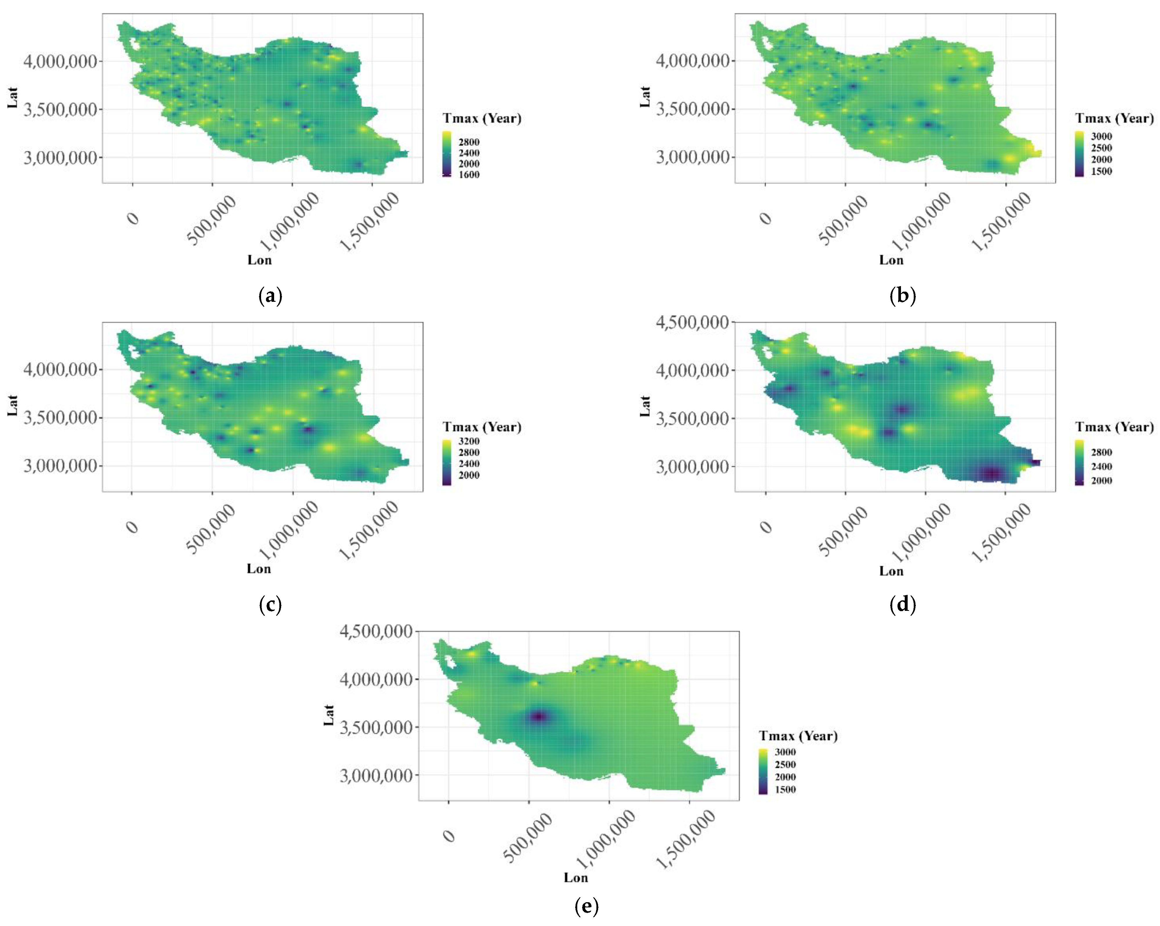Figure 13 displays the combined maximum return period of droughts and floods at approximately 3200 years, with a minimum of approximately 1500 years, highest in the north and west and lowest in the central and southern areas.

3.9. Ensemble Model Under SSP585 for 2071–2100

This study reviews drought and flood forecasting using downscaled river flow data from the Ensemble model under the SSP585 scenario. Figure S39 shows the predicted maximum drought intensity via a deep learning model for 2071–2100, indicating severe droughts starting at −300, approximately 400% higher than near-future estimates. Figure S40 illustrates drought intensity variations for different SDIs, with the highest values in the southeastern and northern areas and the lowest in the southwest. Figure S41 forecasts maximum drought duration for 2071–2100 at approximately 300 months, a 445% increase compared to earlier periods. Figure S42 illustrates drought durations for various SDIs, with the longest in the northeast and shortest in the south and southwest. Figure S43 predicts peak flood flow from the Ensemble model for 2071–2100 to be over 4000 m³/s, a 20% decline from near-future values. Figure S44 estimates peak flood flows post-drought for different SDIs, with the highest in the northwestern and northeastern regions. Figure S45 indicates drought–flood intervals exceeding 6 months, a 72% drop from near-future predictions, peaking from 2098 to 2100. Figure S46 outlines intervals between floods and droughts from 1 to 4 months, with the highest in the west and northeast, and the lowest in the south and southeast. Figure 14 shows maximum return periods for concurrent drought and flood events to be from 250 to 450 years, with the highest in western and eastern regions and the lowest in central and southern areas. Figure S41 again forecasts maximum drought duration for 2071–2100, confirming that it exceeds subsequent years at 300 months—a 445% rise. Figure S42 details drought duration variations for different SDIs, replicating previous findings. Figure S43 predicts maximum flood flow for 2071–2100 to be over 4000 m³/s, a 20% decline from earlier values. Figure S44 depicts maximum flood peaks after droughts, ranging from 0 to 600 m³/s for SDI1 to 0 to 60 m³/s for SDI12, with the highest flooding peaks in the northwestern and northeastern regions.

3.10. Vulnerability

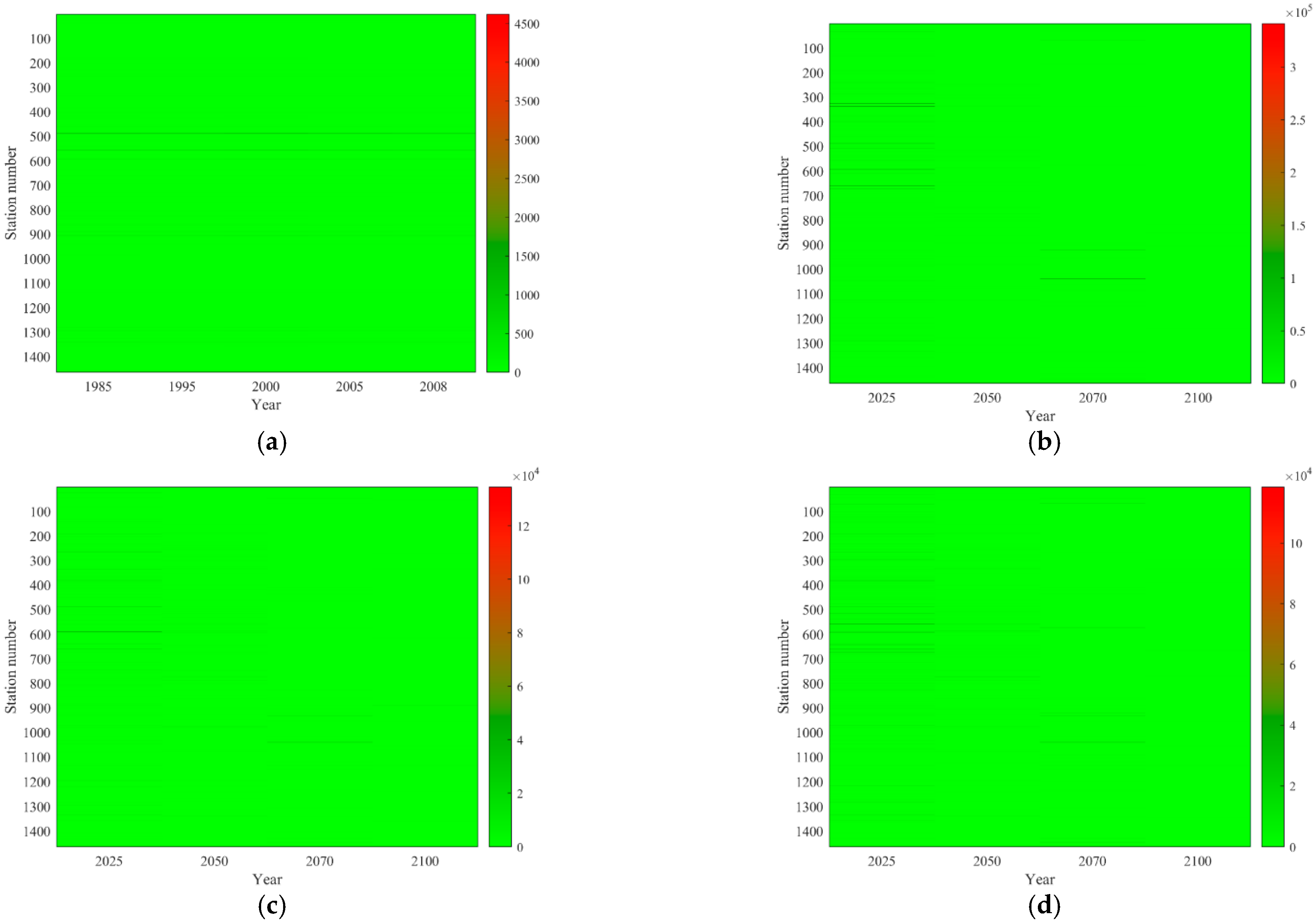
The results of the changes in the vulnerability criterion are illustrated in Figure 15 for the Ensemble model. In this figure, the vulnerability values for the years 2025, 2050, 2071, and 2100 are reported at 1464 stations. Based on this figure, the maximum vulnerability values are calculated as 3 in 10⁵, 12 in 10⁴, and 10⁵ for the SSP126, SSP370, and SSP585 scenarios, respectively. For these scenarios, the highest vulnerability value is estimated for the year 2025. These maximum values are predicted to be approximately 6700% higher than the base period (maximum vulnerability of about 4500).

In this study, the combined effect of drought and flood was projected based on integrating U-Net++ with machine learning algorithms and QM. The U-Net++QM outperformed other integrated models. Based on the downscaled results of U-Net++, there is a bias in the outputs of this model. QM, based on probabilistic methods and considering the distribution of observational data, corrects the bias of downscaled results. Machine learning algorithms require various features to correct bias in this problem. Hence, in this study, QM outperformed machine learning algorithms. This method was successful in the bias correction of GCM outputs in different studies, such as [30,40,41,42].

The results of projecting the combined effect of flood and drought were different for each GCM and emission scenario. This can be attributed to the uncertainty in GCMs and related scenarios that arise from different assumptions and characteristics (Table 1 and Table 2). These variations are for changes in river flow in future periods (Figure 7). The mentioned uncertainty was shown by fuzzy uncertainty analysis in Figure 8. In this figure, GFDL had less uncertainty. In other studies [29,43,44], this model was employed as a tool for climate change projection in Iran.

With multivariate probabilistic analysis of the combined effects, the spatial variations for the SDI differed across different time scales. This was because of differences in the statistical parameters of the SDI time series across different time scales and, consequently, in the probabilistic analysis. The vulnerability results show distinct spatial and temporal variations for different models and scenarios. However, the vulnerability index values differ across the models and scenarios. This is because of the different values for the characteristics of the combined phenomena of flood and drought, as well as different values for the economic and social parameters.

The spatial variations in drought and flood intensity are due to differences in Iran’s topography, distance from the sea, and latitudinal zones. In the mountainous region, where fluctuations in various climate parameters are common, distinct characteristics of flooding and drought are evident.

The results of this study reveal an increase in vulnerability of the combined effects of flood and the future period compared to the base period. This issue may be attributed to increases in drought severity, drought duration, and flood peaks, which decrease the time interval between drought and flood events. Moreover, spatial and temporal variations in GDP can yield different vulnerability values.

4. Conclusions

This study introduced an integrated method to predict the spatial–temporal compound events of floods and droughts. It used gridded flow data from ISIMIP3b for the base period (1985–2014), near future (2021–2050), and far future (2071–2100) as inputs, while using observational discharge data from hydrometric stations as the target variables. A regression relationship was established between ISIMIP3b outputs and river flows using the U-Net++ deep learning, quantile mapping methods, and machine learning techniques for downscaling. River flows were predicted for both future periods, and uncertainty was assessed with the fuzzy method. Drought and flood characteristics were extracted, and multivariate statistical analysis based on copula functions determined the return period of compound events. Finally, vulnerability values were calculated for both the base and future periods. The drought and flood events were assessed by drought severity, duration, peak flood discharge, and the interval between them. The best algorithm for downscaling ISIMIP3b data in the GFDL, MRI_ESM2, and UKESM1 models was the U-Net++QM algorithm (by up to 58% less RRMSE). Fuzzy uncertainty analysis shows less uncertainty for the GFDL-ESM4.

The results of the combined drought–flood effect study for this model indicate that, in the near future, the values of maximum drought intensity and drought duration are expected to decrease. In contrast, flood peak flow is expected to increase, and the time interval between drought and flood events is also expected to increase. In the far-future period, the maximum predicted values for drought intensity increased, drought duration increased, flood peak flow decreased, and the time interval between drought and flood increased. The return period of the combined drought and flood phenomena also increased for future periods (from 50 to 250 years to 50–1000 years). Based on the vulnerability results for the models and scenarios, the years 2071 and 2025 exhibit a higher level of vulnerability compared to the base period years and the year 2100.

The framework and results of this study can help in planning for decreasing the damage from floods and droughts in climate change conditions.