Abstract
The continuous growth of the social economy and the accelerated urbanisation process have led to a rising increase in the demand for water resources in river basins. The uneven temporal and spatial distribution of water resources has further exacerbated the contradiction between supply and demand. The traditional extensive water resource allocation model is no longer suitable for the diverse demands of sustainable development in river basins. Therefore, there is an urgent demand to determine how to reconcile the supply and demand of water resources in river basins to achieve a rational allocation. Taking the Yellow River Basin as an example, an optimal water allocation framework based on multi-objective robust optimisation method was proposed in this study. A robust constraint boundary conditions for the industrial, agricultural, construction and service, ecological, and social water demand were selected from the perspective of the economy–society–ecology nexus. Then, Latin hypercube sampling was adopted to modify the Monte Carlo method to improve the dispersion of sampling values for quantifying the uncertainty of water allocation parameters. Furthermore, a multi-dimensional spatial equilibrium optimal allocation combining adjustable robust optimisation and multi-objective optimisation was established. Finally, a multi-objective particle swarm optimisation algorithm based on a crossover operator was constructed to obtain the Pareto-optimal solution for multi-dimensional spatial equilibrium optimal allocation. The primary findings were as follows: (1) Parameter uncertainty had a significant effect on the provincial/regional revenues of water resources but has no obvious effect on basin revenue. (2) The uncertainty in runoff and parameters had a significant influence on decisions for optimal water allocation. The optimal volume of water purchased by different provinces (regions) varied greatly under different scenarios.
1. Introduction
Water resources are indispensable foundational natural resources and strategic economic assets crucial for human survival and socioeconomic development. The high ratio of sewage generation and discharge, low efficiency of water resource utilisation, and uneven temporal and spatial distribution present significant challenges for current basin water resource management [1,2,3]. Numerous studies have demonstrated that optimal water allocation (OWA; water rights trading) is an effective means of optimising sustainable development strategies, enhancing water-use efficiency, and mitigating the uneven temporal and spatial distribution of water resources through market-based mechanisms [4,5]. The simulation and optimisation process for OWA requires the construction of mathematical models and estimation of parameters and coefficients. This process introduces uncertainties related to variables, such as sewage discharge volumes, sewage treatment costs, and revenues derived from water resource utilisation. Owing to cognitive limitations, the values of these parameters and coefficients often differ from actual conditions, resulting in outcomes derived from abstract parameter calculations that do not accurately represent real-world situations [6,7]. These uncertainty factors impact the OWA process within the basin under an economic–social–ecological equilibrium framework. Despite these challenges, significant progress has been made in the analysis of parameter uncertainty and the optimisation of water allocation. The details of their findings are as follows.
In OWA research, Fu et al. [8] developed an interval two-stage stochastic programming model to enhance the economic value of a water resource system while introducing penalty terms and risk control mechanisms. Wang et al. [9] developed a two-stage stochastic programming water allocation model based on Bayesian optimisation for the Yingke District. Wang and Guo [10] developed an interval multistage stochastic programming model to optimise water resource allocation in the study area. They improved the accuracy of the linkage and conditional distribution functions in water allocation by establishing functional equations between water demand and optimistic-pessimistic factors. Zhang and Li [11] achieved a balance between improving water quality and optimising water allocation by integrating interval two-stage and interval water quality models. Naghdi et al. [12] established an OWA model for the joint scheduling of surface and groundwater in irrigation districts using interval two-stage stochastic programming and multi-objective optimisation methods.
In the realm of uncertainty analysis in basin water allocation, the fuzzy mathematical theory addresses the vague uncertainties inherent in water resource systems, thereby advancing research on uncertainty within the field of water resource management. Lu et al. [13] introduced the fuzzy set theory for water resource management under uncertain conditions and proposed an interval two-stage fuzzy stochastic programming method. Wang and Huang [14] embedded an interactive fuzzy decomposition module within the framework of interval two-stage stochastic programming, and proposed an interactive two-stage stochastic fuzzy programming method. Nematian [15] improved the two-stage stochastic programming using fuzzy chance constraints to address OWA problems under uncertainty. Nematian [16] developed an interval two-stage stochastic programming water allocation model that incorporated fuzzy chance constraints, thereby validating the effectiveness of fuzzy chance-constrained programming. A remarkable limitation of the aforementioned interval two-stage fuzzy stochastic programming model is its inability to consider multiple and mixed uncertainties in the parameters of the problem; that is, the combination of interval, probability, and possibility distributions [17,18].
The aforementioned studies extensively analysed and discussed the application of two-stage stochastic programming methods, interval programming methods, and fuzzy theory in OWA for basins. However, these methods still face challenges in adapting and balancing multiple uncertainty scenarios for optimal solutions and do not consider the economy–society–ecology-coupled boundary constraints in the concept of sustainable basin development.
In recent years, robust optimisation methods have provided new approaches for addressing uncertain optimisation problems in linear programming. To address the potential conservativeness of robust optimisation methods, Ali et al. [19] proposed an improved robust optimisation method that flexibly adjusts the conservativeness level of robust solutions, thereby achieving widespread application in uncertainty research across various fields. Zhu et al. [20] integrated interval programming, fuzzy membership functions, and robust optimisation methods into a general framework, and proposed an interval parameter fuzzy robust nonlinear programming method to address river water quality management under uncertain conditions. Nasiri et al. [21] constructed a robust multi-objective bargaining model to balance the water resource allocation among basins under uncertain conditions. Dadmand et al. [22] applied sustainability evaluation indicators to a water resource allocation model, establishing a robust fuzzy stochastic water resource allocation model that was applied to a water-scarce city in Iran, yielding robust water resource allocation results. These studies demonstrated that robust optimisation methods can effectively address uncertainty issues in OWA. However, existing robust optimisation methods typically solve the most conservative scenario under the same robustness criteria and lack a mechanism to adjust the preference between high-yield and conservative decisions. Therefore, it is of great relevance to study the matching supply and demand for OWA for sustainable development in the Yellow River Basin (YRB) from the perspective of uncertainty analysis and the economy–society–ecology nexus [23,24].
Therefore, the main objectives of this study are (1) maximising the revenue of water resources in the YRB with the consideration of uncertainty quantification and competition among different water right individuals, (2) maximising the revenue of water resources in each region (province) of the YRB, (3) as well as providing equilibrium solutions for optimal trading quantity of water (OTQW) in each region (province). The main contributions and innovations of this study are as follows:
(1) A quantitative method of parameter uncertainty of water allocation in the YRB was constructed to improve the dispersion of sampling values with the combination of the Monte Carlo method and Latin hypercube sampling (LHS).
(2) Considering parameter uncertainty, scenario uncertainty and relative robustness criteria in the YRB, a two-layer optimal water allocation model combining adjustable robust optimisation and multi-objective optimisation was established, and the corresponding comprehensive value of water resources (CVWR) was calculated.
(3) To obtain the multi-objective optimal equilibrium solutions under uncertain conditions in the YRB and to avoid falling into the local optimal problem, an improved multi-objective particle swarm optimisation (PSO) algorithm was introduced by linearly combining particles from the particle population and elite set to implement the crossover operator of real-coded genetic algorithms.
This paper is organised as follows. Section 2 describes the structure and theoretical analysis of OWA model in the YRB based on quantitative method of parameter uncertainty, adjustable robust optimisation mechanism, and improved multi-objective particle swarm. Section 3 introduces the overview of the study area, data source, and parameter setting. Section 4 presents results and discussions, and Section 5 gives conclusions.
2. Methodology
2.1. Research Framework
The objective of the optimal allocation of water resources for sustainable development in the YRB is to seek the equilibrium solution of maximising the comprehensive value of water resources. The framework of the demand–supply matching model for the optimal allocation of water resources for sustainable development in the YRB proposed in this study is illustrated in Figure 1. The modelling process of this framework involves three functional sub-modules: quantitative analysis of parameter uncertainty in water allocation for sustainable development, construction of the OWA model considering uncertainty and the economy–society–ecology nexus, and model solving based on a multi-objective particle swarm.
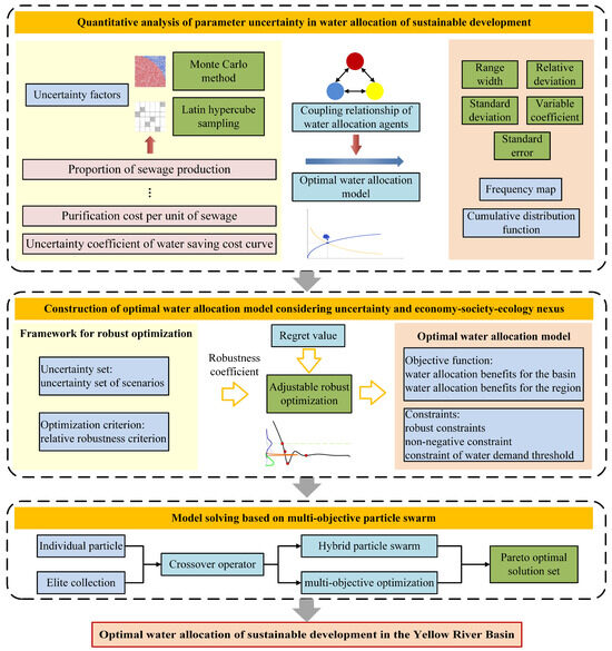
Figure 1.
Research framework of the overall methodology proposed in this study.
Quantitative analysis of parameter uncertainty in water allocation for sustainable development: First, we identified the uncertainty factors that may impact water allocation for sustainable development in the YRB (e.g., sewage generation ratio, unit sewage treatment cost, and uncertainty coefficient of water-saving cost curves). Therefore, to enhance the dispersion of sampled values in traditional uncertainty analysis methods, the Monte Carlo method was improved using LHS, which increased the diversity of the sampling results. This approach allowed for a quantitative analysis of the uncertainties in water allocation for sustainable development in the YRB. The performance indicators for the uncertainty analysis included range width, relative deviation, standard deviation, coefficient of variation, and standard error.
Construction of the OWA model considering uncertainty and economy–society–ecology nexus (OWA-UESE): The dominant economy–society–ecology relationships in the objective functions of water allocation at the basin and regional levels were clarified. Subsequently, a set of scenario uncertainties and relatively robust criteria were selected, and a water allocation model that combines adjustable robust optimisation and multi-objective optimisation was established to seek the equilibrium solution of maximising the comprehensive value of water resources at the basin and regional levels. Robust coefficients were introduced to balance system revenues under various uncertainty scenarios, thereby reducing the impact of parameter uncertainty on water allocation for sustainable development in the YRB.
Model solving based on multi-objective PSO: To overcome the problem of traditional PSO algorithms falling easily into local optima, the particles of the individual and elite sets were linearly combined to achieve the crossover operator of the real-coded genetic algorithm. This increased the exchange of information between the particles. Based on this, a multi-objective PSO algorithm incorporating the crossover operator was constructed to solve the Pareto optimal solutions for the water allocation model for sustainable development in the YRB from the perspectives of uncertainty analysis and the “economy–society–ecology” balance.
2.2. Basic Theory
2.2.1. Participants and Uncertain Factors of Water Allocation for Sustainable Development in the YRB
Participants in water allocation for sustainable development in the basin include basin water administrative agencies, provincial (regional) water administrative agencies, and water rights exchanges. Basin water administrative agencies do not directly participate in the decision-making process of water allocation, but instead coordinate sustainable water allocation among provinces (regions) through administrative regulations in the form of water rights trading. Provincial (regional) water administrative agencies directly participate in the decision-making process of water rights trading, and water rights exchanges provide a platform for these trades.
Sources of uncertainty in water allocation for sustainable development in the basin include the natural environment, social economy, engineering technology, institutions, markets, and subjective factors of water rights trading entities. The primary uncertainties analysed in this study for water allocation for sustainable development in the YRB include the unit value of water resources, ratio of sewage generation, unit cost of sewage treatment, unit consumption value of untreated sewage, uncertainty coefficient of the value curve, and uncertainty coefficient of the water-saving cost curve.
2.2.2. Mathematical Theoretical Methods for Uncertainty Analysis
Complex systems often contain many uncertain parameters. To address parameter uncertainty, probabilistic statistical methods use mathematical definitions and reasoning to construct a mature framework for quantification. Among these methods, the Monte Carlo method effectively simulates stochastic characteristics and is suitable for quantitative analysis of uncertainties in complex systems [23,24].
The main steps for performing an uncertainty analysis of the OWA model for sustainable development in the basin are shown in Figure 2. First, random numbers that conform to the uncertainty distribution were generated for each uncertainty parameter, and the process was repeated multiple times to construct a sample set of uncertainty parameters. Each set of samples was used as an input parameter for the OWA model for sustainable development in the basin, and the output results were collected to quantify the range of the impact of uncertainty.
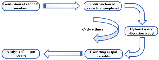
Figure 2.
Monte Carlo method diagram.
The purpose of Latin hypercube sampling (LHS) [25] is to ensure that the sample points cover the complete distribution interval of the variables, addressing the clustering defect in the sample results generated by simple random sampling in the Monte Carlo simulation process. The method involved the following steps:
- (1)
- Random sampling
Assume that N samples must be drawn in an M-dimensional vector space . The cumulative probability distribution function of variable in the i-th dimension is , as shown in Figure 3. For each , the curve was evenly divided into N equidistant intervals based on the function values. In each of the N intervals, a simple random sampling was conducted to obtain N values. Therefore, the sample points obtained in this manner achieved a complete coverage over the entire sampling interval.
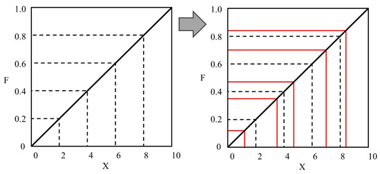
Figure 3.
LHS method diagram of random sampling.
- (2)
- Permutation and combinations
For each , the N sampled values were randomly permuted. The sampling results for each were combined, grouping together the values with the same permutation order to obtain an N-sample M-dimensional vector set .
Figure 4 shows the process and results of drawing five samples in a two-dimensional vector space according to the above steps.
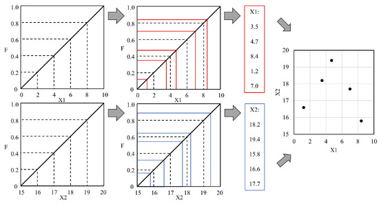
Figure 4.
LHS method diagram of premutation and combinations.
2.2.3. Adjustable Robust Optimisation Method
The robust optimisation method effectively addresses the impact of uncertainty on the results of water allocation for sustainable development in basins. Robust optimisation solutions demonstrate a strong resistance to uncertainty.
In optimal programming models, the uncertainty of real-world problems is mainly manifested in the uncertainty of the input parameter values. In robust optimisation, uncertainty sets are used to describe this uncertainty. An uncertainty set contains all possible input parameter values, and common types include scenario, interval, likelihood, and relative entropy uncertainty sets. A scenario uncertainty set, which refers to the uncertain parameters that take values in several finite scenarios, is a simple convex hull uncertainty set.
The selection of the optimal criteria involves the construction of a robust objective function. There are three robust optimisation criteria: absolute robustness, robust deviation, and relative robustness [26]. These criteria differ in their definitions of “better” and “worse” decisions.
Absolute Robustness Criterion
For a given decision, its objective value under each combination of input parameter values is computed and the worst objective value is used as the performance measure of the decision. This approach selects the optimal decision for the problem by solving for the optimal (minimum objective value) solution under the worst (maximum objective value) input–parameter combination. Therefore, the absolute robustness criterion is known as the minimax criterion. The decision obtained by the absolute robustness criterion optimisation is called an absolutely robust decision. The specific expression for an absolutely robust decision is as follows.
where is the optimal objective function value corresponding to the robust decision , s is the scenario corresponding to a combination of input parameter values, is the robust decision, X is the feasible domain of decision x, is the instance of input parameter values under scenario s, S is the set of all scenarios, and is the objective function of the deterministic model with respect to x under the input parameter instance .
Robust Deviation Criteria
According to the robust deviation criterion, the optimal objective value was first calculated for each combination of the input parameter values. Subsequently, for a given decision, the difference between its objective value under each combination of input parameter values and the optimal objective value for the corresponding combination was calculated, with the largest difference used as the performance measure for that decision. This approach selects the optimal decision for the problem by determining the optimal (minimum regret value) solution for the worst (maximum regret value) combination of input parameters, which is a form of the minimax regret criterion. The regret value is defined as the difference calculated using the above process.
The robust deviation decision is specifically expressed as follows:
where is the optimal objective function value corresponding to the robust decision, is the optimal decision of the deterministic model for the input parameter instance , and is the optimal objective value of the deterministic model for the input parameter instance .
The established robust deviation programming model is as follows.
Relative Robustness Criteria
The relative robustness criterion is another form of the minimax regret criterion, which defines the regret value as the deviation percentage between the objective value of the decision under a combination of input parameter values and the optimal objective value of the corresponding parameter value combination. First, the optimal objective value for each combination of input parameter values is calculated, and then, for a particular decision, its regret value under each combination of input parameter values is calculated. The maximum regret value is used as the performance measure for that decision. This approach selects the optimal solution for a problem by determining the optimal (minimum regret value) solution for the worst (maximum regret value) combination of input parameters.
The relatively robust decision is specifically expressed as follows:
where is the robust decision corresponds to the robust optimal objective function value.
The established relatively robust programming model is shown as follows.
All three robustness criteria aimed to determine the optimal value under the worst parameter combination, representing the most conservative situation under the same robustness criterion. In practical applications, decision makers have their own preferences for high-yield and conservative decisions. Therefore, adjustable robust optimisation is proposed, adjusting the conservativeness of robust optimisation through the robust coefficient ρ.
A robust programming model in the general form must be transformed before it can be solved. When the uncertainty set is continuous, the robust constraint is equal to an infinite number of constraints, rendering it directly unsolvable. It is necessary to transform the original robust constraint and use duality theory to convert the original robust linear programming problem into a robust counterpart problem. In this study, the OWA problem for sustainable basin development was transformed into a relatively robust programming model with discrete scenario uncertainty sets, and the adjustable relatively robust planning was constructed as follows.
where z is the optimal objective function value of the scenario uncertainty set with adjustable relatively robust programming and is the probability of scenario s occurring. denotes the robust coefficient.
2.3. OWA Model for Sustainable Development Guided by Uncertainty and Economy–Society–Ecology Nexus
A scenario uncertainty set was selected to represent uncertainty in the OWA model for sustainable development. According to Section 2.2.1, the uncertainty factors selected in the YRB include the unit value of water resources, proportion of sewage generated, unit cost of sewage treatment, unit value of untreated sewage consumption, uncertainty coefficient of the value curve, and uncertainty coefficient of the water-saving cost curve. By combining the possible values of these uncertainty parameters, the value curve, and the uncertainty coefficient of the water-saving cost curve, we established the possible OWA parameter scenarios and the corresponding occurrence probabilities for the basin, constructing the scenario uncertainty set S to describe the uncertainty of the OWA in the basin.
2.3.1. Two-Layer OWA Model Based on Adjustable Robust Optimisation Mechanism
The goal of the basin is to maximise revenue for the basin water administrative department, specifically maximising the total value of water resources and tax revenue from water rights transactions. Maximising the total value of water resources involves maximising economic, social, and ecological environmental values while minimising the negative value of water pollution.
Each province (or region) in the basin aims to maximise its regional revenue, which involves maximising the total value of water resources and transaction revenue in the region while minimising various cost expenditures. These expenditures include water saving, wastewater treatment, and tax expenditures.
A unified unit water resource trading price is set for the entire basin as a whole in the utilisation of water resources. During the water allocation process in the basin, each province formulates the trading price based on the supply and demand relationship, achieving economic value compensation for the traded water volume among the provinces. The total amount of water resources purchased by the buyer in the monetised water resources transaction is equal to that of the seller. Therefore, the total CVWR value of the basin will not be affected by the price of water resource transactions.
Based on this analysis, the OWA model for sustainable development in the YRB was structured as a two-layer model. Because the revenues of the same water allocation decision vary across different scenarios and differ from the optimal revenues of each scenario, the relative robust criterion was adopted as the robust optimisation criterion of the model. The adjustable relative robust optimisation of the scenario uncertainty set is applied to the OWA of the basin, establishing a multi-objective OWA model for sustainable development that considers uncertainty and the economy–society–ecology nexus, as detailed below.
The objective functions of the model are formulated as follows.
where is the robust optimal target revenue value of the basin, is the robust optimal target revenue value of province (region) i, is the probability of scenario s occurring, is the total revenue of the basin under scenario s when the OWA decision is made, and is the total income of province (region) i under scenario s of water rights trading decisions. and are calculated as follows.
where denotes the value curve uncertainty coefficient of scenario s, and represents the five water usage sectors: industry, agriculture, construction and services, society, and ecological environment, respectively. denotes the value curve parameter of the h-th industry in the i-th province (region), is the unit water resource value of the h-th industry in the i-th province (region) under the condition of no water saving in scenario s. represents the water-saving amount of the i-th province (region). is the initial water rights of the i-th province (region) in scenario s. is the water allocation ratio of the h-th industry in the i-th province (region). is the water rights trading volume of the i-th province (region), with a positive value indicating the purchase of water rights, and a negative value indicating the sale of water rights. represents the negative value per unit of untreated sewage and is the sewage treatment rate of the i-th province (district). is the sewage discharge coefficient of the h-th industry in the i-th province (region). is the tax revenue of the basin in scenario s. is the benchmark price of water rights trading in scenario s, set as the highest unit water resource value among the water rights sellers. reflects the impact of trading activity on prices and . is the uncertainty coefficient of the water-saving cost curve and is the water-saving investment cost required for water-saving amount . is the tax expenditure of the i-th province (region) in scenario s. is the unit sewage treatment cost of the i-th province (region) in scenario s. In the water resource reallocation plan, the affected user groups are classified into n categories (such as agriculture, industry, low-income residents, etc.), denoted as l = 1, 2, …, n. Then, the formula for calculating the total opportunity cost is . denotes the reduced water volume for the i-th category of users due to reallocation. represents the unit water output loss value of the i-th type of user. denotes the unit water substitution cost of the i-th type of user. represents the transaction price per unit of water of province i. If the province is the seller, the value of is positive. If the province is the buyer, the value of is negative. The total allocated water volume in province i is .
, , and represent economic value, social value, and ecological environment value per unit of water in province i, respectively. The proportions of water applied to economic, social, and ecological environment values in province i can be denoted as , , and , respectively. Then, economic value, social value, and ecological environment value of water resources can be calculated by , , and [27].
The constraint conditions of the normal optimal model are as follows.
Equations (14) and (15) are robust constraints that limit the regret value of a decision to less than the robust coefficient . is the optimal revenue value of the basin in scenario s and is the optimal revenue value of the i-th province (region) in scenario s. is the water demand threshold of the h-th water usage sector in the i-th province (region) under scenario s. represents the historical annual water-saving amount of the i-th province (region). denotes the actual water volume after trading of the h-th water usage sector in the i-th province (region) under scenario s. represents environmental flow after the implementation of the water allocation plan in the YRB, denotes the minimum water demand threshold for environmental flow of the YRB.
2.3.2. Model Solving Based on Improved Multi-Objective Particle Swarm
PSO is known for its fast convergence speed. However, it has the drawback of easily falling into local optima. By linearly combining particles from the particle population and elite set to implement the crossover operator of real-coded genetic algorithms, the exchange of information among particles is increased. This approach can overcome the disadvantage of PSO by easily falling into local optima. Based on this, this study employs a multi-objective PSO algorithm that incorporates a crossover operator for model solving [27]. The attributes of the objects and population objects in the proposed algorithm are detailed in Table 1 and Table 2, respectively.

Table 1.
Attribute declarations of multi-objective PSO.
Table 2.
Correspondence between different functions and modules.
The key operators of multi-objective particle swarm optimisation include the particle encoding operator, the velocity–position update operator, and the external archive operator. The particle encoding operator divides the basin into 9 major water users according to administrative divisions, and the encoding must meet the basic water use constraints of the basin. The inertia weight of the velocity–position update operator is taken from the adaptive value (initially 0.9, linearly decreasing to 0.4 with the number of iterations). The individual learning and group learning weights are set to be equal to ensure that particles can not only refer to their own historical optimal solutions but also absorb the group’s optimal solutions. The external archive operator uses the “crowding distance sorting method” to maintain the archive: when a new solution is added, the dominated solutions are deleted first; if the archive is full (set capacity to 100), the crowding distance of each solution is calculated (the smaller the distance, the denser the distribution of the solution), and the solution with the smallest crowding distance is deleted. This operator ensures that the final output of the optimal solution set is evenly distributed. The weights of the first and second layer OWA objective functions are 0.6 and 0.4, respectively; that is, the maximisation of regional water allocation benefits must be subordinate to the maximisation of the overall water allocation benefits of the basin management institution.
The water resources system is subject to inherent uncertainties (such as fluctuations in runoff and deviations in water demand predictions). This study adopts a combined approach of “historical data statistics + expert validation” to determine these. The “mean ± standard deviation” of monthly runoff from 2010 to 2023 is calculated, and “mean ± 30%” is taken as the uncertainty range (as the maximum inter-annual variation in runoff in the YRB reaches 30%) [5].
- Particle velocity and position iteration
For the k-th iteration, for the i-th particle in the population, the velocity and position of the particle are and , respectively. The optimal position of the particle is , and the optimal position of the population is . The particle velocity and position were updated as follows.
where denotes the position of a particle randomly selected from the elite population set. , , and are random numbers ranging from 0 to 1, and , , and are fixed values representing the inertia weights of the particle velocity, self-learning factor, and social learning factor, respectively.
- Uncontrolled rank value sorting
For a population of size N, where is a particle in the population, uncontrolled rank value sorting was performed according to the following steps:
(1) Set .
(2) Select a particle from P and let .
(3) For each particle in population P, and .
Let .
For each particle in , determine the controlled relationship of the particle fitness function values:
① If , ,;
② If , no processing is performed;
③ If and , when , .
Let .
(4) Output a subpopulation of the same uncontrolled rank, whose rank value is .
(5), if , then end, otherwise, set and jump to step (2).
- Updating the crowding degree of particles in subpopulations
For each subpopulation, of the population sorted by uncontrolled rank values: Let it have m objective functions, iterate T times, and calculate the crowding degree of the particles in the subpopulation according to the following steps:
(1) Set , and initialise the crowding degree distance for all particles.
(2) For each objective function :
Sort each particle in the sub-population P by the value of the objective function, ;
Crowding distance between the first particle and the n-th particle in subpopulation P:
The crowding distance for second particle to the n − 1th particle in the sub-population P:
(3) If , then end, otherwise, set and jump to step (2).
- Improved multi-objective PSO
The solution steps of the multi-objective PSO algorithm based on the crossover operator are as follows:
(1) Set , initialise the population with N particles.
(2) Perform uncontrolled rank sorting on , calculate the crowding degree distance for each particle, update the elite set of the population, and update the Pareto optimal solution set of the problem.
(3) Randomly select a particle from the elite set as the particle corresponding to the global optimal position of the population, update the velocity and position of each particle in the population , and generate population .
(4) Generate a new population .
(5) Perform uncontrolled rank sorting on , calculate the crowding degree distance for each particle in the sub-population, and select N particles according to the principle of “priority to particles with higher uncontrolled rank, and for particles with the same uncontrolled rank, priority to particles with larger crowding degree distance.”
(6) Set , and form the new generation population with the particles selected in step (5).
(7) Update the elite set of population .
(8) Update the Pareto optimal solution set of the problem: let , perform uncontrolled rank sorting on A, and select particles with higher uncontrolled rank to form set A.
(9) End when , output the Pareto optimal solution set of the problem; otherwise, proceed to step (3).
In step (3), by determining the controlled relationship of the particle fitness function value, the particle’s optimal position is selected as follows:
(1) Set the initial condition of the individual best particle corresponding to the particle optimal position as each particle in the initial population , and set the new particle generated after updating the velocity and position as .
(2) If , then retain .
(3) If , then .
(4) If and , randomly select to retain or let .
Throughout the algorithm, constraints are handled as follows. Whenever a Pareto dominance comparison is performed between two particles, we first check whether the two particles satisfy the constraint conditions. Particles that satisfied the constraints and had fewer constraint violations were preferentially selected. When both particles satisfied the constraint conditions, a Pareto dominance comparison was performed, and the particle with the Pareto dominance was preferentially selected. The optimal value of the model solving algorithm is determined by Tamhane test [28]. Meanwhile, the algorithm parameters are optimised by Response Surface Methodology (RSM) [29].
3. Case Study
3.1. Overview of the Study Area
The Yellow River originates in the Bayan Har Mountains in Qinghai Province and flows through nine provinces (regions): Qinghai, Sichuan, Gansu, Ningxia, Inner Mongolia, Shaanxi, Shanxi, Henan, and Shandong. It finally empties into the Bohai Sea in Kenli County, Dongying City, Shandong Province, as shown in Figure 5. Most of the YRB is located in arid and semi-arid regions with low precipitation and high evaporation. The water resources of the basin are primarily replenished by atmospheric precipitation, leading to severe water resource shortages. The multi-year average runoff is 58 billion m3, with a per capita water resource of 905 m3. The YRB is a crucial ecological barrier and a grain production area in China. To meet the needs of socioeconomic development, the water resource development and utilisation rate in the basin should be as high as 80%, ranking first among the 10 major river basins in China. Economic development levels in different regions of the YRB vary significantly, resulting in differing degrees of water resource development and utilisation among the provinces (regions). Consequently, the value of water resources varies across provinces (regions). OWA, including mechanisms such as water rights trading, can achieve an efficient flow of water resources within the basin, addressing disparities in water resource availability and utilisation.
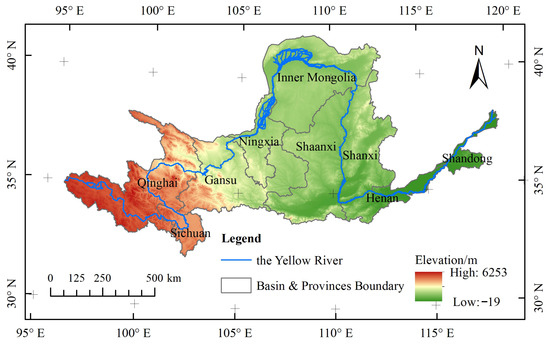
Figure 5.
Yellow River and administrative divisions.
3.2. Data Source and Parameter Setting
According to the Comprehensive Planning of the Yellow River Basin (2012–2030) and China Water Resources Bulletin [30], the water resource allocation results from the implementation of the South-to-North Water Diversion Project’s eastern and central routes before the implementation of the first phase of the western route were used as the initial benchmark water rights allocation results, as shown in Table 3.
Table 3.
Initial water rights allocation in the YRB in 2020 (unit: 100 million m3).
Based on the historical water-saving amounts and historical water-saving investment data from the Statistical Yearbook of each province (region) in the YRB, the curve parameter fitting method was adopted and the corresponding parameter values of the water-saving cost functions for each province (region) were obtained, as listed in Table 4.
Table 4.
The parameter values of the water-saving cost functions for each province (region) in the YRB.
According to the rigid water demand forecast results from the Comprehensive Planning of the Yellow River Basin (2012–2030) and China Water Resources Bulletin [30], the minimum water demand thresholds for each water-use sector were obtained, as shown in Table 5.
Table 5.
Water demand thresholds of each water-use sector for each province (region) in the YRB (unit: m3).
4. Results and Discussion
4.1. Sensitivity Analysis of Uncertain Factors in the OWA-UESE Model of the YRB
The uncertain parameters in this study include the runoff volume, water pollution treatment process, the process of producing value from water resources, and the uncertain parameters involved in the process of saving water: the proportion of wastewater generation, the unit cost of wastewater treatment, the value of untreated water consumption per unit, the unit value of water resources, the uncertainty coefficient of the value curve, and the uncertainty coefficient of the water-saving cost curve. On this basis, the Monte Carlo simulation method based on LHS of the OWA-UESE was adopted to generate sample sets. Then, 1000 sets of uncertainty parameter samples were generated within the range of −5% to +5% based on the benchmark values. Three tax modes were selected: taxing the buyer based on trading revenue (Tax mode 1), taxing the seller based on trading revenue (Tax mode 2), and taxing the buyer and seller based on trading revenue (Tax mode 3). The uncertainty parameter samples were input separately to the two-layer OWA model based on adjustable robust optimisation mechanism for the solution, and the results were optimised according to the improved multi-objective particle swarm in Section 2.3.2. In the process of model solving based on improved multi-objective particle swarm, the initial particle number is set to 1000 and iterated 1000 times. Then, the optimal water rights trading results of each scenario are obtained and statistically compared.
4.1.1. Sensitivity Analysis of Uncertain Runoff on the Revenue of the Basin
Table 6 presents the influence of the uncertainty of the runoff volume on the total benefit of the basin OWA-UESE when the runoff volume varies within the range of [−30%, 30%]. It can be seen from the table that when the runoff volume fluctuates by 30% above and below the benchmark value, the sensitivity varies within the range of [−8.3%, 6.9%], and all remain below 8.5%. This indicates that the two-layer OWA model based on the adjustable robust optimisation mechanism proposed in this study has strong robustness.
Table 6.
Sensitivity analysis of runoff volume during the process of variation in the uncertain interval.
4.1.2. Analysis of the Impact of Uncertainty on the Revenue of Provinces/Regions
For tax mode 1 (tax on buyers), the two-layer OWA model is constructed based on adjustable robust optimisation mechanism (Equations (10)–(13) in Section 2.3.1) and the corresponding optimal revenue values for each province (region) in the YRB are calculated based on improved multi-objective particle swarm (Equations (21)–(25) in Section 2.3.2). The optimal revenue values for each province (region) under uncertain conditions are listed in Table 7. From the distribution range of the samples in each province (region), it is evident that the parameter uncertainty significantly affects the water allocation revenue of each province within the basin. The variation ranges of the samples relative to the benchmark values are [−98.0%, 236.6%] and [−92.0%, 112.8%], with the coefficient of variation ranging from [7.7%, 32.5%].
Table 7.
The optimal revenue of each province (region) under the condition of tax mode 1.
The cumulative distribution function (CDF) curves of revenue for each province (region) under tax mode 1 are shown in Figure 6. For Qinghai, Gansu, Shanxi, and Shandong, the baseline values corresponded to CDF curve values > 0.75, indicating that the revenues of most samples are lower than the benchmark values. If the parameter uncertainty is not considered, the probability of overestimating the revenues of these provinces (regions) is >75%. For Ningxia and Henan, the benchmark values correspond to CDF curve values of <0.25, suggesting that, if parameter uncertainty is not considered, the probability of underestimating the revenue of these provinces (regions) is >75%.
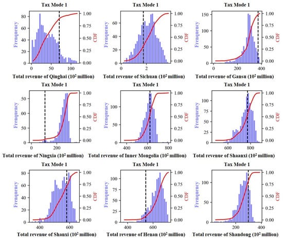
Figure 6.
Revenue calculation results of provinces (regions) under the condition of tax mode 1.
4.1.3. Analysis of the Impact of Uncertainty on the Total Revenue
Without considering uncertainty, the benchmark values of total basin revenue under the tax mode 1, 2, and 3 were CNY 357.44 billion, CNY 357.35 billion, and CNY 357.70 billion, respectively, with the highest revenue achieved when taxing the buyer and seller and the lowest revenue when taxing the seller. The calculated results of the total basin revenue under the three tax modes when considering uncertainty are shown in Figure 7. When taxing the buyer, the total basin revenue ranged from 340.02 billion to CNY 377.10 billion, with a relative change range from the benchmark value of −4.9% to 5.5%. When taxing the seller, the total basin revenue ranged from CNY 339.76 billion to CNY 376.70 billion, with a relative change range from the benchmark value of −4.9% to 5.4%. When taxing the buyer and seller, the total basin revenue ranged from CNY 340.33 billion to CNY 377.13 billion, with a relative change range from the benchmark value of −4.9% to 5.4%. Under all tax modes, the total basin revenue of the samples showed a uniform distribution, with a change range of approximately ±5.0%, indicating that parameter uncertainty had no significant impact on the total basin revenue.
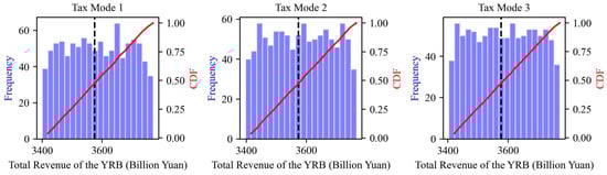
Figure 7.
Distribution of total regional revenue calculation results under different tax modes.
The sum of the revenues for each province (region) was calculated as the total revenue of the region. Without considering uncertainty, the benchmark values of total regional revenue under tax modes 1, 2, and 3 were CNY 337.10 billion, CNY 337.32 billion, and CNY 339.81 billion, respectively, with the highest revenue achieved when taxing the buyer and seller and the lowest revenue when taxing the buyer. The calculated results of the total regional revenue under the three tax modes when considering uncertainty are shown in Figure 8. When taxing the buyer, the total regional revenue ranged from CNY 319.75 billion to CNY 357.94 billion, with a relative change range from the benchmark value of −5.1% to 6.2%. When taxing the seller, the total regional revenue ranged from CNY 318.54 billion to CNY 358.32 billion, with a relative change range from the benchmark value of −5.6% to 6.2%. When taxing the buyer and seller, the total regional revenue ranged from CNY 319.22 billion to CNY 357.23 billion, with a relative change range from the benchmark value of −6.1% to 5.1%. Under all tax modes, the total regional revenue of the samples showed a uniform distribution, with a change range of approximately ±5.0%, indicating that parameter uncertainty had no significant impact on the total regional revenue.
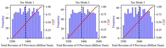
Figure 8.
Distribution of total basin revenue calculation results under different tax modes.
4.2. Construction of Parametric Scenario Set and Computation of Robust Constrained Boundary Conditions
4.2.1. Construction of Parametric Scenario Set
Based on the uncertainty levels of the runoff volume, pollution, value, and water-saving cost, as well as the potential scenarios, seven possible water rights trading scenarios were set, as shown in Table 8. The statistic possibilities of each scenario were captured primarily from the China Water Resources Bulletin [30]. Scenarios 1 and 2 represent the worst conditions (i.e., lowest runoff volume, highest pollution consumption, lowest value, and highest water-saving cost) and optimal conditions (i.e., highest runoff volume, lowest pollution consumption, highest value, and lowest water-saving cost), respectively, with probabilities set at 0.1. Scenario 3 was the most likely scenario, with the runoff volume at the normal water year level and other parameters set to actual values, with probabilities set at 0.2. Scenarios 4 and 5 represent the conditions of the lowest runoff volume with the best other parameters and the highest runoff volume with the worst other parameters, respectively, with probabilities set at 0.15. Scenarios 6 and 7 are scenarios that may occur in a normal water year with probabilities set at 0.15. Scenario 6 represents the conditions with the highest pollution consumption, highest value, and lowest water-saving costs, whereas Scenario 7 represents the conditions with the lowest pollution consumption, lowest value, and highest water-saving costs.
Table 8.
The setting of the uncertainty scenario.
This study used the 2020 level year runoff volume of 51.98 billion m3 from the Comprehensive Planning of the Yellow River Basin (2012–2030) as the normal water year runoff volume, with the corresponding initial water rights allocation results as the initial water rights allocation results for a normal water year. Based on this, the classification of the runoff volume abundance and drought levels in the YRB is presented in Table 9. The ratio of the average runoff volume of the Yellow River during slightly rainy years to that during normal water years was 1.250 and that during slightly dry years to that during normal water years was 0.851. Considering that water rights trading is unsuitable in extremely drought and extremely rainy years, this study sets the dry year runoff volume as the 2020 level year runoff volume of 51.98 billion m3 converted at a ratio of 0.851, and the rainy year runoff volume as the 2020 level year runoff volume of 51.98 billion m3 converted at a ratio of 1.250. The initial water rights allocations for the drought, normal, and abundant scenarios set in this study are listed in Table 10.
Table 9.
Classification of natural runoff rainy and drought levels in the Yellow River.
Table 10.
Results of initial water rights allocation in the basin under different runoff volumes (unit: 108 m3).
The high and low values corresponding to the proportion of sewage generated, unit sewage treatment cost, untreated sewage consumption value, and unit water resource value are derived from the original data multiplied by factors of 1.15 and 0.85, respectively. Similarly, the uncertainty coefficients for the value curve and the water-saving cost curve are set to high and low values of 1.15 and 0.85, respectively.
4.2.2. Computation of Robust Constrained Boundary Conditions
Taking Scenario 2 (rainy year in the basin) as an example, all uncertainty parameters were set to their optimal values (minimum pollution consumption, highest unit value of water resources, and lowest water-saving costs). The parameter scenario setting in Section 4.2.1 is substituted into the OWA model in Section 2.3.1, and the improved multi-objective particle swarm in Section 2.3.2 is adopted to optimise the solution. On this basis, a set of Pareto solutions for a deterministic multi-objective water rights trading model was obtained. Ten Pareto-optimal solutions are selected based on the optimal conditions for each goal, as shown in Figure 9. Water rights sellers include Inner Mongolia, Henan, Shanxi, and Ningxia, with a total water rights volume of 23 billion m3 before trading. Water rights buyers include Shandong, Shaanxi, Gansu, Qinghai, and Sichuan, with a total water rights volume of 17.8 billion m3 before trading. The total transaction volume of water rights was 3.05 billion m3, accounting for 13.3% of sellers’ total water rights before the transaction and 14.6% of buyers’ total water rights after the transaction. The proportion of water rights held by sellers changed after the water rights transactions. Shanxi sold 1.34 billion m3 of water rights, accounting for 43.9% of the total transaction volume, making it the seller with the most water rights sold. After the transaction, Shanxi’s water rights holdings were lower than those of Ningxia, which sold 826 million m3 of water rights. Furthermore, the rankings of water rights holdings in Inner Mongolia, Henan, Shandong, and Sichuan remained unchanged.
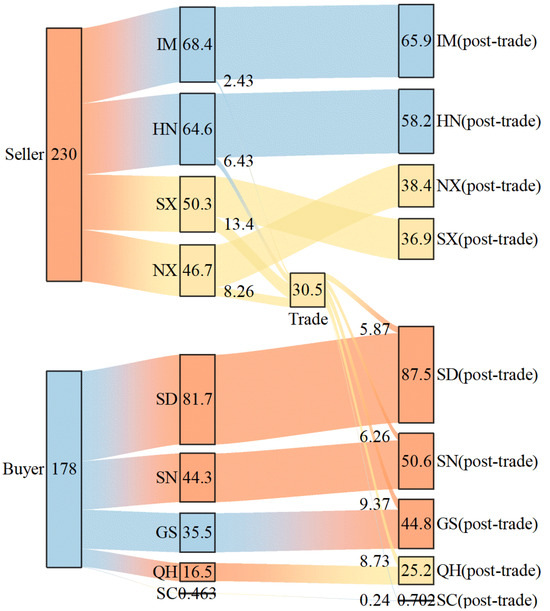
Figure 9.
Sankey diagram of OWA decisions in a basin under Scenario 2 (unit: 100 million m3).
According to the calculation results of each scenario, a combination of optimal values of each objective function was selected as the input parameter F* for the robust constraint conditions required for the subsequent robust water rights trading model solution, as shown in Table 11.
Table 11.
The calculation results of robust constraint input parameter F* (unit: CNY 100 million).
The optimal water rights trading volumes for each scenario are shown in Figure 10. Positive values indicate the volume of water rights purchased, whereas negative values indicate the volume of water rights sold. S1-1 represents the first optimal solution for Scenario 1. There were differences in the trading volumes of the YRB. The maximum value was 5.84 billion m3, accounting for 14.3% of the total initial water rights, and the minimum value was 597 million m3, accounting for 2.1% of the total initial water rights. Scenario 5 was a rainy year with the largest water rights trading volume, whereas Scenario 1 was a dry year with the smallest trading volume. As the runoff volume increased, the proportion of trading water volume to the total initial water rights also increased, indicating that the runoff volume had the greatest impact on the activity level of water rights trading. Compared with Scenario 2, which was also a rainy year, Scenario 5 had a higher trading volume. This is because, under the same inflow conditions, worsening parameters such as water-saving costs force trading entities to use water rights trading more actively to increase their revenues. Similarly, for the scenarios representing normal years, the water rights trading volumes in Scenarios 3 and 7 are similar, whereas Scenario 6 has the least trading volume. This indicates that value is the direct driving factor for water rights trading and that water-saving costs have a smaller impact on the level of activity in water rights trading.
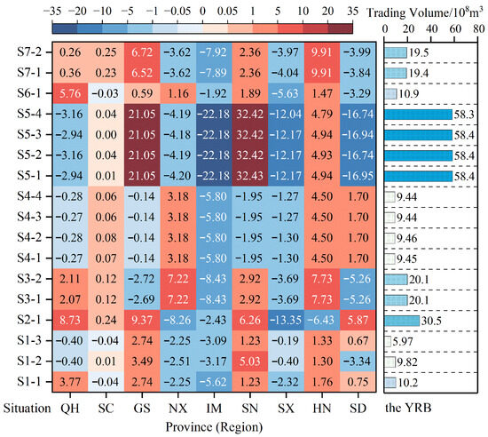
Figure 10.
Comparison diagram of water rights trading under different scenarios.
There were significant differences in the water rights of Inner Mongolia and Shanxi under different scenarios. The minimum and maximum volumes sold by Inner Mongolia were 192 million m3 and 2.218 billion m3, respectively, with a standard deviation of 560.2 million m3 and a coefficient of variation of 81.8%. The minimum and maximum volumes sold by Shanxi were 19 million m3 and 1.335 billion m3, respectively, with a standard deviation of 460 million m3 and a coefficient of variation of 91.5%. The trading roles of some provinces (regions) in the basin have changed, and there are significant differences in trading volumes, even when the trading roles are the same. The minimum and maximum purchase volumes in Shaanxi were 120 million m3 and 3.12 billion m3, respectively, with a coefficient of variation of 138.8%, making it the province (region) with the largest variation in water rights trading volume. In summary, when faced with multiple scenarios of runoff volumes and water rights trading parameters, the decisions made by provinces (regions) vary greatly. In practice, only one decision can be made and a robust constraint condition is required to determine the decision that can achieve optimal results under various scenarios.
4.3. Analysis of Robust Optimisation Decision Results of the OWA-UESE Model
By setting the robustness coefficient to 0.5, the OWA models in the YRB and each province were reconstructed and calculated by improved multi-objective particle swarm and then a Pareto set satisfying the robustness constraints was obtained, and two typical Pareto decisions with the worst and best robustness were selected. The optimal trading water and water-saving volumes for each province (region) are shown in Figure 11a and Figure 11b, respectively.
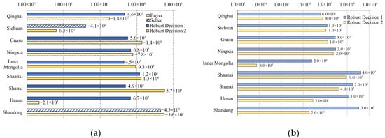
Figure 11.
Pareto optimal robust decision. (a) Optimal volume of water rights traded (unit: m3); (b) optimal water-saving amount (unit: m3).
As shown in Figure 11a, in decision 1, Sichuan and Shandong are sellers, whereas Qinghai, Gansu, Ningxia, Inner Mongolia, Shaanxi, Shanxi, and Henan are buyers. The total water rights traded in the entire basin volume was 451.8 million m3, accounting for 8.08%, 6.88%, and 5.50% of the total water rights of sellers in dry, normal, and rainy years, respectively. Inner Mongolia is the province (region) with the lowest volume of water rights purchased, with a purchase volume of 44.6 million m3, accounting for 9.88% of total traded water rights. It also had the smallest proportion of purchased water rights after the transaction, accounting for 0.95%, 0.81%, and 0.39% of the total water rights in Inner Mongolia after transactions in dry, normal, and rainy years, respectively. Compared with other provinces (regions), water rights transactions bring lower revenue to Inner Mongolia, resulting in low enthusiasm for water rights trading in Inner Mongolia.
In decision 2, Qinghai, Gansu, Ningxia, Henan, and Shandong are sellers, whereas Sichuan, Inner Mongolia, Shaanxi, and Shanxi are buyers. Compared with those in decision 1, where almost all the sold water volume comes from Shandong alone, the sources of traded water rights in decision 2 are more diverse. Shanxi is the province (region) with the most traded water rights and the largest proportion of purchased water rights after the transaction, accounting for 71.79% of total traded water volume. This represents 14.26%, 13.90%, and 6.74% of the total water rights in Shanxi after the transaction in the dry, normal, and rainy years, respectively. At this time, the revenue Shanxi gains from purchasing water rights exceeds the costs, indicating a high willingness to purchase more water rights to obtain value revenue.
As shown in Figure 11b, the water-saving amounts in decisions 1 and 2 for Qinghai, Sichuan, Gansu, and Ningxia are similar. However, the water-saving amounts for Inner Mongolia, Shaanxi, Shanxi, Henan, and Shandong differ significantly, with the water-saving amounts of Inner Mongolia differing by three orders of magnitude. Overall, the water-saving amount in decision 2 was less than that in decision 1, corresponding to a higher water rights trading volume in decision 2. These two decisions have different preferences for water rights trading and saving. Decision 1 focused on increasing value through water saving to enhance overall revenue, making it a water-saving decision. decision 2 focused on redistributing water resources through water rights trading to enhance the overall revenue, making it a trading decision. The total water-saving amount in decision 1 was 1.1529 billion m3, with Shaanxi having the highest water-saving amount, accounting for 37.00% of the basin’s total water-saving amount. The total water-saving amount in decision 2 was 196.8 million m3. The water-saving amount of Inner Mongolia was the lowest, indicating that it has low water-saving potential and high water-saving costs, and the revenue from continuously increasing the water-saving amount is less than the corresponding water-saving costs. As shown in Equations (14)–(20), in the OWA-UESE model, the minimum water demand thresholds for the economic, social, and ecological environment aspects of water resources are clearly defined. Meanwhile, the equilibrium of water supply and demand among provinces within the basin and the maximisation of the comprehensive value (economic–social–ecological environment) are set as the solution objectives. Therefore, the above robust optimal solutions in this section undoubtedly reconcile supply and demand under the economic–social–ecological environment nexus in the process of maximising the comprehensive value of water allocation.
4.4. Comparative Analysis of Total Revenue Before and After OWA-UESE Model Decision
The distribution of expected total revenue and value for each province (region) before and after water rights trading in the YRB is shown in Figure 12. For Trading Scenario 1, the expected revenues of Qinghai, Gansu, Ningxia, Inner Mongolia, Shaanxi, Shanxi, and Henan provinces decreased, the expected revenues of Sichuan and Shandong increased, and the expected revenues of Sichuan and Shandong increased. This is because Robust Solution 1 is a water-saving decision. Substantial water-saving efforts in each province (region) result in significant water-saving costs, leading to decreased expected revenues in most provinces (regions). However, these provinces (regions) increase their expected total value through water-saving behaviours. For Trading Scenario 2, the expected revenues of Inner Mongolia, Shaanxi, Shanxi, and the three provinces (regions) decreased, whereas the expected revenues of Qinghai, Sichuan, Gansu, Ningxia, Henan, and Shandong increased. The trading role significantly impacts revenue. Generally, buyers purchase water rights to increase the value of water resources and their revenue decreases because of the cost of purchasing water rights, whereas sellers benefit from selling water rights, thereby increasing their revenue. However, Sichuan has low water-saving costs and its water-saving behaviour increases the unit value of water resources. After purchasing water rights, Sichuan gained more water resource value, leading to an increase in revenue, even as a water rights buyer. Robust Solution 2 is a trading decision, where water rights trading increases the expected total revenue of several provinces (regions); however, the total expected value of water resources in certain provinces (regions) decreased. The total expected value of water resources in Qinghai, Gansu, Ningxia, and Shandong decreased by CNY 35 million, CNY 242 million, CNY 70 million, and CNY 812 million, respectively.
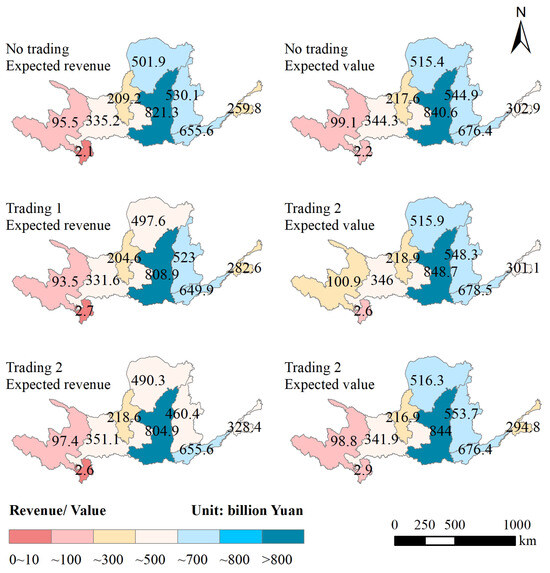
Figure 12.
Distribution diagram of expected total revenue for each province (region).
The distribution of the expected water-saving costs and tax expenditures for each province (region) is shown in Figure 13. The water-saving amount in the water-saving decision (Trade 1) was markedly larger than that in the trading decision (Trade 2). For Trade 1, Shandong and Shaanxi had the highest water-saving costs of CNY 1.27 billion and CNY 1.05 billion, respectively. Shandong and Shaanxi had the highest water-saving amounts. For Trade 2, Shaanxi and Shanxi had the highest water-saving costs of CNY 190 million and CNY 140 million, respectively. Shaanxi and Shanxi had the highest water-saving amounts.
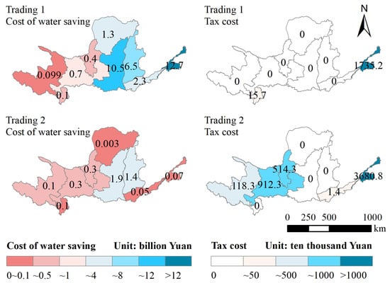
Figure 13.
Distribution diagram of expected water-saving costs and tax expenditures for each province (region).
Tax expenditure in the trading decision (Trade 2) was substantially larger than that in the water-saving decision (Trade 1). In Trade 1, only Sichuan and Shandong were water rights sellers, and the basin collected water rights trading taxes only from these two provinces (regions). For Trade 2, Qinghai, Gansu, Ningxia, Henan, and Shandong were water rights sellers, and the basin collected water rights transaction taxes from these five provinces (regions). Shandong had the largest volume of water rights sales; therefore, its tax expenditure was the highest.
As shown in Figure 14, the social value of water resources in the YRB before trading is CNY 104.56 billion, accounting for 29.5% of the positive value of water resources in the YRB. In Trading Scenarios 1 and 2, the social value of water resources in the YRB increased by CNY 354 million and CNY 67 million, respectively, reaching CNY 104.91 billion and CNY 104.63 billion, respectively. After Trade 1, the ecological environment value of water resources in the YRB significantly improved, increasing from CNY 30.53 billion before trading to CNY 31.00 billion, an increase of CNY 465 million, with the highest relative increase rate of 1.52%. Negative revenue related to sewage includes the negative value brought about by untreated sewage and the cost of sewage treatment. After water rights trading, the negative revenues related to sewage decreased from CNY −13.39 billion before trading to CNY −13.26 billion, reducing by CNY 132 million. After water rights trading, the economic, social, and ecological environmental values of water resources in the YRB improved and the negative revenues related to sewage decreased.
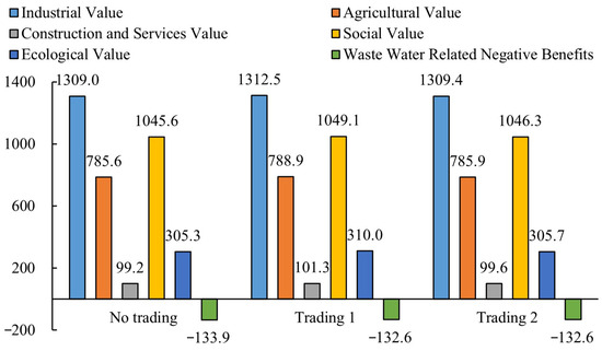
Figure 14.
Comparison of expected revenue situations for water resource values in the YRB.
The CVWR statistics of each province in the calculation basin are shown in Table 12. The CVWR index value of this study is significantly better than the historical allocation plan of the YRB. This is because the optimal water allocation model of this study, under the premise of fully considering the water demand threshold constraints of each sector, has achieved the maximisation of the economic benefits of water resource utilisation.
Table 12.
The CVWR statistics of different schemes.
4.5. Comparative Analysis of the Results of the Robust Optimisation and Deterministic Models
We substitute the average of all uncertain parameters into the OWA model in Section 2.3.1 and solve it using the improved multi-objective particle swarm method in Section 2.3.2. Then, the calculation result of the deterministic model can be acquired. Compare this result with the solution of the proposed OWA-UESE model under uncertain conditions. The river basin revenue corresponding to the robust and deterministic model decisions for various scenarios is shown in Figure 15. If water rights trading is carried out without considering the uncertainty of parameters, it may result in some provinces (regions) having less water after the trade, which cannot meet the water demand threshold of each water-using department, thus bringing risks to the water resources system of the Yellow River Basin. Therefore, the deterministic model decision results obtained with the initial determined values of parameters are not reliable, and the benefits are obtained under the premise of system risks, while robust decision-making will not cause violation of constraints. The ranking of river basin revenue situations from high to low across different scenarios is as follows: Scenarios 2, 7, 4, 3, 5, 6, and 1. Scenario 2, with the best inflow situation and parameters, exhibited the highest total river basin revenue, whereas Scenario 1, which had the worst inflow situation and parameters, and had the lowest total river basin revenue. The revenue in Scenario 4 surpassed that in Scenario 5, indicating that the cumulative impact of the uncertainty parameters was greater than that of the inflow volume. Additionally, the revenue in Scenario 7 exceeded that in Scenario 6, suggesting that the uncertainty of water-saving costs has a smaller impact on the total river basin revenue than the uncertainty of pollution and water resource value.
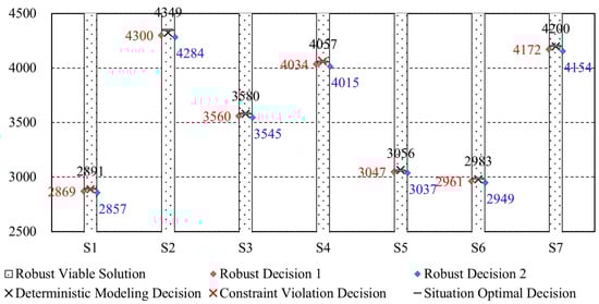
Figure 15.
Total basin revenue corresponding to robust decision-making (unit: CNY 100 million).
4.6. Comparison Between Previous Studies and the OWA-UESE Model
The proposed model solving method based on improved multi-objective particle swarm (IMPS) is compared with the typical meta-heuristic algorithms, such as particle swarm optimisation (PSO) [31] and differential evolution algorithm (DEA) [32]. The comprehensive value of water resources (CVWR) was quantified based on the Equations (10)–(13) in this study.
Considering the practical demands of water allocation in the Yellow River Basin, this study adopts a dual convergence criterion of “iteration termination condition (hard constraint) + convergence index threshold (soft constraint)”. The maximum number of iterations is set at 200. When the number of iterations exceeds 200, the uniformity of the distribution of Pareto solutions improves by less than 3%, but the computational time increases by more than 20%. The soft constraint conditions for convergence iteration are set as the generation distance ≤ 0.01 and the rate of change in the reverse generation distance for five consecutive generations ≤ 1%. The number of particles is 100, the external archive capacity is 100, the initial inertia weight and the final inertia weight are 0.9 and 0.4, respectively. The crowding distance threshold is 0.05.
The running time of the meta-heuristic algorithms and the corresponding CVWR value are shown in Figure 16. Figure 16a indicates that the CVWR result of the IMPS solution is obviously better than PSO and DEA, and the amplitude is higher than 7%. This is because IMPS can realise the crossover operator of real coded genetic algorithm by the linear combination of the particle individual and elite set of particles, increase the information exchange between particles, and overcome the shortcomings of PSO and DEA which can fall easily into local optimal. As shown in Figure 16b, the running time of IMPS and PSO is basically the same. However, DEA convergence speed is slow; the time is more than 12% higher than other algorithms. From the above analysis, it can be seen that it is appropriate to adopt IMPS for optimisation solutions.
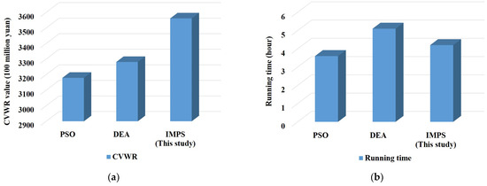
Figure 16.
Comparison of the running time and CVWR value of the meta-heuristic algorithms. (a) CVWR values based on different meta-heuristic algorithms; (b) statistics of the running time of the meta-heuristic algorithms.
To analyse the performance of different optimal water allocation schemes, the administrative management-based water allocation mechanism (AM-RWRAP) [33] and the OWA for water rights trading in the basin (OWA-with respect to) [34] (Wang, 2011) were introduced to compare with the OWA-UESE model. Equations (10)–(13) were adopted to quantify the comprehensive value of water resources (CVWR) in the YRB. According to the quantification of scenario probability in Table 7 and parameter uncertainty, the CVWR quantification method in Equation (12) was adopted for calculation, and the statistical results of each water resources allocation scheme were obtained and presented in Figure 17.
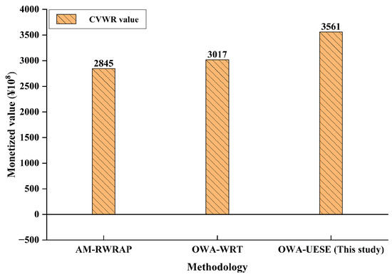
Figure 17.
CVWR distribution of the YRB in different water allocation schemes (unit: CNY 100 million).
As shown in Figure 17, the calculated values, which include economy, society, ecological environment, and sediment transport, are combined with the YRB data in 2023 and the trading cycle T is set to 1 year. The CVWR value of the OWA-UESE model is significantly higher than that of other models (AM-RWRAP and OWA-with respect to). This is because other models do not take into account the uncertainty parameters of different scenarios and the negative value of sewage on CVWR, and the improved multi-objective particle swarm method enhances the accuracy of solving the optimal solution for water distribution.
The optimisation model of this research provides a technical path for the efficient allocation of water resources in the YRB. However, its practical application urgently requires supporting policies and market mechanisms. Therefore, we suggest establishing a basin water rights trading platform with total control and rights confirmed for water-using departments of each province. First, the basin management institution must complete the initial water rights confirmation and registration under the premise of ensuring the ecological water demand threshold and the water use red line of each province, laying a legal foundation for the trading. Secondly, a multi-level trading market should be established, allowing water-using departments such as agriculture and industry to trade their surplus water on the online platform, and the government should set a price range to prevent market failure. Most importantly, the platform should utilise real-time monitoring and remote metering technologies to ensure the traceability and verifiability of the traded water volume, thereby establishing a sustainable market-based water resource allocation system.
5. Conclusions
Based on the above research model of optimal water allocation in the YRB, the following conclusions can be drawn:
- (1)
- The robust solutions of the two-layer OWA-UESE model across all scenarios indicate that the economic, social, and ecological values of water resources in the Yellow River Basin (YRB) have increased, while the negative revenues associated with sewage treatment have decreased significantly.
- (2)
- The ranking of river basin revenue situations from highest to lowest across different scenarios is as follows: Scenarios 2, 7, 4, 3, 5, 6, and 1. This indicates that the cumulative impact of uncertainty parameters was greater than that of basin inflow volume, and that the uncertainty in water-saving costs has a relatively smaller effect on total river basin revenue compared to the uncertainties in pollution and water resource value.
- (3)
- Since IMPS can implement the crossover operator of a real-coded genetic algorithm through a linear combination of particle individuals and the elite set of particles, thereby enhancing information exchange among particles and overcoming the tendency of PSO and DEA to fall into local optima, the CVWR result of the IMPS solution in this study is significantly better than those of PSO and DEA, with an improvement exceeding 7%. Moreover, the runtime of IMPS is comparable to that of other metaheuristic algorithms. Therefore, the two-layer OWA-UESE modelling framework in the Yellow River Basin (YRB) can enhance strategic trade-offs in efforts to ensure basin water sustainability and revenue maximisation under diverse scenarios and uncertainties.
The robust optimisation solutions in this multi-objective framework depends on the objective functions of the basin administrative agency and each province. Therefore, the proposed OWA-UESE may be extended to various stakeholders and can be applied with limited modification to other basins that face similar water management problems and have a strong unified administration.
Author Contributions
D.D. and Q.S.: conceptualisation, formal analysis, funding acquisition, investigation, methodology, project administration, supervision, validation, visualisation, writing—original draft, writing—review and editing; H.H. and S.D.: data curation, formal analysis, investigation, methodology, software, validation, visualisation; H.W.: software, visualisation, data curation; L.X.: funding acquisition, project administration, resources. All authors have read and agreed to the published version of the manuscript.
Funding
This work was supported in part by the National Natural Science Foundation of China 42477172, by Henan Province scientific and technological innovation talents in college and university 24HASTIT026, by Youth Support Program of the China Association for Science and Technology CHINCOLD-QNRC0010, by Natural Science Foundation of Henan Province 252300421086, by Key Research and Development Project of Henan Province 251111220700, by the Youth Talent Promotion Project of Henan Province 2024HYTP033, by Program for Innovative Research Team (in Science and Technology) in University of Henan Province 23IRTSTHN004, by Key Program of Science and Technology Research Plan Joint Foundation of Henan Province 235200810014, by Natural Science Foundation of Henan Province 242300421001, and by Leading Talent Program for Central Plains Basic Research 22ZYLJ005.
Data Availability Statement
Data will be made available on request.
Conflicts of Interest
The authors declare that they have no known competing financial interests or personal relationships that could have appeared to influence the work reported in this paper.
References
- Zhang, H.; Luo, J.; Wu, J. Dynamic multiobjective two-stage fuzzy stochastic strategy for optimal water allocation in inter-basin water division under changing environment: A case study of Hanjiang-to-Weihe water division in Shaanxi Province, China. J. Clean. Prod. 2024, 452, 142175. [Google Scholar] [CrossRef]
- Zhang, Y.; Lu, Y.; Zhou, Q. Optimal water allocation scheme based on trade-offs between economic and ecological water demands in the Heihe River Basin of Northwest China. Sci. Total Environ. 2020, 703, 134958. [Google Scholar] [CrossRef] [PubMed]
- Li, M.; Xu, Y.; Fu, Q. Efficient irrigation water allocation and its impact on agricultural sustainability and water scarcity under uncertainty. J. Hydrol. 2020, 586, 124888. [Google Scholar] [CrossRef]
- Guo, H.; Chen, X.; Liu, J. Joint analysis of water rights trading and water-saving management contracts in China. Int. J. Water Resour. Dev. 2020, 36, 716–737. [Google Scholar] [CrossRef]
- Huang, Q.; Lv, C.; Feng, Q. Stackelberg game based optimal water allocation from the perspective of energy-water nexus: A case study of Minjiang River, China. J. Clean. Prod. 2024, 464, 142764. [Google Scholar] [CrossRef]
- Wei, F.; Zhang, X.; Xu, J. Simulation of water resource allocation for sustainable urban development: An integrated optimization approach. J. Clean. Prod. 2020, 273, 122537. [Google Scholar] [CrossRef]
- Feng, J. Optimal allocation of regional water resources based on multi-objective dynamic equilibrium strategy. Appl. Math. Model. 2021, 90, 1183–1203. [Google Scholar] [CrossRef]
- Fu, Q.; Li, L.; Li, M. An interval parameter conditional value-at-risk two-stage stochastic programming model for sustainable regional water allocation under different representative concentration pathways scenarios. J. Hydrol. 2018, 564, 115–124. [Google Scholar] [CrossRef]
- Wang, Y.; Yin, H.; Guo, X. Distributed ANN-bi level two-stage stochastic fuzzy possibilistic programming with Bayesian model for irrigation scheduling management. J. Hydrol. 2022, 606, 127435. [Google Scholar] [CrossRef]
- Wang, Y.; Guo, P. The interval copula-measure Me based multi-objective multi-stage stochastic chance-constrained programming for seasonal water resources allocation under uncertainty. Stoch. Environ. Res. Risk Assess. 2021, 35, 1463–1480. [Google Scholar] [CrossRef]
- Zhang, Q.; Li, Z. Development of an interval quadratic programming water quality management model and its solution algorithms. J. Clean. Prod. 2020, 249, 119319. [Google Scholar] [CrossRef]
- Naghdi, S.; Bozorg-Haddad, O.; Khorsandi, M. Multi-objective optimization for allocation of surface water and groundwater resources. Sci. Total Environ. 2021, 776, 146026. [Google Scholar] [CrossRef]
- Lu, H.; Huang, G.; Zeng, G. An inexact two-stage fuzzy-stochastic programming model for water resources management. Water Resour. Manag. 2008, 22, 991–1016. [Google Scholar] [CrossRef]
- Wang, S.; Huang, G. Interactive two-stage stochastic fuzzy programming for water resources management. J. Environ. Manag. 2011, 92, 1986–1995. [Google Scholar] [CrossRef] [PubMed]
- Nematian, J. An extended two-stage stochastic programming approach for water resources management under uncertainty. J. Environ. Inform. 2016, 27, 72–84. [Google Scholar] [CrossRef]
- Nematian, J. A two-stage stochastic fuzzy mixed-integer linear programming approach for water resource allocation under uncertainty in Ajabshir Qaleh Chay Dam. J. Environ. Inform. 2023, 41, 52–66. [Google Scholar] [CrossRef]
- Hao, N.; Sun, P.; Yang, L. Optimal allocation of water resources and eco-compensation mechanism model based on the Interval-Fuzzy Two-Stage Stochastic Programming method for Tingjiang River. Int. J. Environ. Res. Public Health 2021, 19, 149. [Google Scholar] [CrossRef]
- Raei, M.; Hossienzad, J.; Ghorbani, M. An uncertainty-based random boundary interval multi-stage stochastic programming for water resources planning. Water Resour. Manag. 2023, 37, 4571–4587. [Google Scholar] [CrossRef]
- Shee, A.; Kopinke, F.; Mackenzie, K. Borohydride and metallic copper as a robust dehalogenation system: Selectivity assessment and system optimization. Sci. Total Environ. 2022, 810, 152065. [Google Scholar] [CrossRef]
- Zhu, H.; Huang, G.; Guo, P. A fuzzy robust nonlinear programming model for stream water quality management. Water Resour. Manag. 2009, 23, 2913–2940. [Google Scholar] [CrossRef]
- Nasiri-Gheidari, O.; Marofi, S.; Adabi, F. A robust multi-objective bargaining methodology for inter-basin water resource allocation: A case study. Environ. Sci. Pollut. Res. 2018, 25, 2726–2737. [Google Scholar] [CrossRef]
- Dadmand, F.; Naji-Azimi, Z.; Farimani, N. Sustainable allocation of water resources in water-scarcity conditions using robust fuzzy stochastic programming. J. Clean. Prod. 2020, 276, 123812. [Google Scholar] [CrossRef]
- Eid, M.; Eissa, M.; Mohamed, E. New approach into human health risk assessment associated with heavy metals in surface water and groundwater using Monte Carlo Method. Sci. Rep. 2024, 14, 1008. [Google Scholar] [CrossRef]
- Yu, J.; Kou, C.; Ma, Y. Effect analysis on hydrocarbon adsorption enhancement of different zeolites in cold start of gasoline engine based on Monte Carlo method. Energy 2024, 294, 130738. [Google Scholar] [CrossRef]
- Trinh, M.; Jun, H. Stochastic bending and buckling analysis of laminated composite plates using Latin hypercube sampling. Eng. Comput. 2023, 39, 1459–1497. [Google Scholar] [CrossRef]
- Tirkolaee, E.; Goli, A.; Faridnia, A. Multi-objective optimization for the reliable pollution-routing problem with cross-dock selection using Pareto-based algorithms. J. Clean. Prod. 2020, 276, 122927. [Google Scholar] [CrossRef]
- Di, D.; Wu, Z.; Wang, H.; Huang, S. Optimal water distribution system based on water rights transaction with administrative management, marketization, and quanti fication of sediment transport value: A case study of the Yellow River Basin, China. Sci. Total Environ. 2022, 802, 1–10. [Google Scholar]
- Brechenmacher, T.; Xu, J.; Dmitrienko, A. A mixture gatekeeping procedure based on the Hommel test for clinical trial applications. J. Biopharm. Stat. 2011, 21, 748–767. [Google Scholar] [CrossRef]
- Chelladurai, S.; Murugan, K.; Ray, A. Optimization of process parameters using response surface methodology: A review. Mater. Today 2021, 37, 1301–1304. [Google Scholar] [CrossRef]
- Di, D.; Wu, Z.; Wang, H.; Huang, S.; Chen, B. Multi-objective optimization for water allocation of the Yellow River basin based on fluid mechanics, emergy theory, and dynamic differential game. J. Clean. Prod. 2021, 312, 127643. [Google Scholar] [CrossRef]
- Freitas, D.; Lopes, L.; Morgado-Dias, F. Particle swarm optimisation: A historical review up to the current developments. Entropy 2020, 22, 362. [Google Scholar] [CrossRef]
- Deng, W.; Shang, S.; Cai, X. An improved differential evolution algorithm and its application in optimization problem. Soft Comput. 2021, 25, 5277–5298. [Google Scholar] [CrossRef]
- Bekchanov, M.; Bhaduri, A.; Ringler, C. Potential gains from water rights trading in the Aral Sea Basin. Agric. Water Manag. 2015, 152, 41–56. [Google Scholar] [CrossRef]
- Wang, Y. Trading water along a river. Math. Soc. Sci. 2011, 61, 124–130. [Google Scholar] [CrossRef]
Disclaimer/Publisher’s Note: The statements, opinions and data contained in all publications are solely those of the individual author(s) and contributor(s) and not of MDPI and/or the editor(s). MDPI and/or the editor(s) disclaim responsibility for any injury to people or property resulting from any ideas, methods, instructions or products referred to in the content. |
© 2025 by the authors. Licensee MDPI, Basel, Switzerland. This article is an open access article distributed under the terms and conditions of the Creative Commons Attribution (CC BY) license (https://creativecommons.org/licenses/by/4.0/).