Abstract
The radius-to-width ratio has an obvious impact on the flow structure within curved channels, which most natural rivers possess, but there are currently few studies on the influence of the radius-to-width ratio of a tributary (R/B) on the hydrodynamic characteristics of a confluent channel. In order to contribute to this field of research, this study employed the RNG k-ε turbulence model, which has good applicability and accuracy for confluence, to investigate the effects of the R/B and flow ratios (q*) on the hydraulic characteristics of confluence. The results reveal that the numerical model can effectively simulate the velocity distribution in the confluence. The values of the key errors are all relatively small (e.g., the value of Mean RMSE is 0.05), and the flow patterns near the bed and water surfaces are different. The maximum velocity zone (MVZ) and the scale of the separation zone (SZ) increase as R/B increases; conversely, the MVZ and the scale of the SZ decrease as the q* increases. Upstream of the confluence, turbulent kinetic energy (TKE) increases and decreases as R/B and q* increase, respectively, while TKE downstream of the confluence hardly changes. Furthermore, the size of the SF decreases as R/B increases. The value of peaks downstream of the confluence, increases with the increase in the R/B, and decreases with the increase in the q*. The results of this study will contribute to a better understanding of the hydrodynamic characteristics of confluence and provide valuable insights for the management and ecological restoration of confluent channels.
1. Introduction
Confluence is an important node in the natural river network, serving as a crucial hub and key site where the river system interacts [1]. The interaction between two flows moving in different directions leads to significant changes in the flow structure, which has a crucial impact on the dispersion of pollutants [2,3], riverbed evolution [4,5], accumulated clutter [6], and morphodynamic processes. Furthermore, the complex flow structure at the confluence also provides habitats for aquatic organisms and enhances the availability of utilizable nutrients. An in-depth understanding of the hydrodynamics of confluent channels is of great significance for pollutant management and ecological governance [7,8].
Currently, the hydrodynamic characteristics of confluent channels have been extensively studied [9,10,11,12]. Previous studies have pinpointed the primary factors influencing confluence, including the junction angle [13], manning coefficient, surface roughness, and flow ratio (q*). Here, q* is defined as Qm/(Qt + Qm), where Qm and Qt denote the main channel and tributary flow rates, respectively. These factors have a significant impact on the SF and SZ, which are two key features of the confluent channel. The SZ is a low-velocity pressure recirculation region located downstream of the confluence (Figure 1c), which alters the pattern of the flow structure, reduces the flow area and flooding passage [14], and has a clear impact on the distribution of energy transfer, velocity, and stress on the riverbed; therefore, it has continuously received attention in relevant research [8,9]. The scale of SZ decreases as the q* increases, and increases as the junction angle increases. Similarly to the spiral motion in the curved channel, secondary flow (SF) is generated downstream of the confluence under the lateral pressure gradient and centrifugal force [5]. The SF alters the velocity distribution and shear stress, thereby influencing the exchange and transfer of substances within the flow field [15]. Furthermore, the generation of SF requires specific conditions: the junction angle, flow ratio, and roughness have an important impact on the evolution and intensity of the SF.
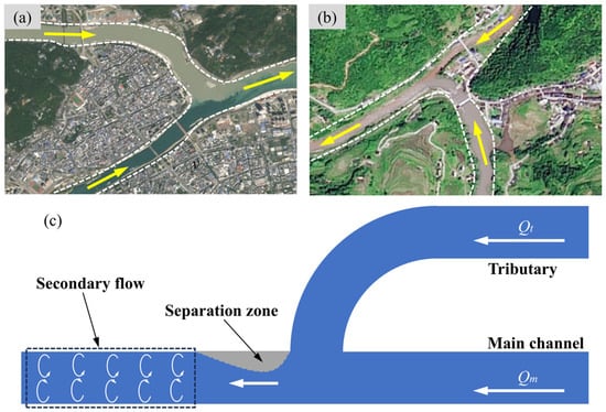
Figure 1.
(a,b) Some confluences with meandering tributaries. (c) Schematic diagram of confluence.
As mentioned above, the effect of flow ratios and junction angles on confluent channels has been extensively studied. However, in some river networks, the tributaries have curved morphologies (Figure 1a,b). Under the combined effect of centrifugal force and the lateral pressure gradient, after the flow moves into the bend, SF will be generated [16,17,18] (Figure 1c). Therefore, the water flow structure within a meandering tributary is completely different from that of a straight tributary, resulting in a more complex water flow structure when the tributary merges into the mainstream. Furthermore, the radius-to-width ratio plays an important role in influencing the flow structure of the curved channel. The velocity distribution within the cross-section becomes increasingly uneven as the radius-to-width ratio decreases. This further intensifies the turbulence of the flow within the bend, resulting in a continuous increase in the turbulent kinetic energy over a wide area downstream of the bend exit. Therefore, the change in the radius-to-width ratio of the meandering tributary has an important impact on the hydrodynamic characteristics downstream of the confluence. However, in current studies of confluent channels, tributaries mostly have straight channel morphologies [19,20,21,22], while there have been relatively few studies on the confluent channels of curved tributaries. This limits our comprehensive understanding and accurate grasp of the hydraulic characteristics of the confluent channels.
To address this knowledge gap, this study employed the RNG k-ε turbulence model to investigate the effects of the R/B and q* on the flow structure (longitudinal velocity, TKE, SZ, and SF) and quantify the longitudinal distribution of the secondary flow intensity. The results will contribute to a better understanding of the hydrodynamic characteristics of confluence, and provide valuable insights for the management and ecological restoration of confluent channels.
2. Description of Numerical Model
2.1. Model Layout and Numerical Cases
The computational model in this study is similar to the equal-width confluence flume of Weber et al. (2001) [19], but has been appropriately adjusted to conduct the research under a wider range of conditions. The computational domain consists of a straight main channel and a curved tributary located on the left side of the main channel. All the channels have a rectangular cross-section with a width (B) of 0.914 m and a height (Z) of 0.56 B (Figure 2a). In order to allow the main channel flow (Qm) and the tributary flow (Qt) to fully develop before they reach confluence, the upstream length of the main channel has been extended to 10 B, the downstream length is 17 B, and the water depth at the entrance of both the main channel and the tributary is 0.34 B. The layout of the confluent channel with different radius-to-width ratios is shown in Figure 2b. The origin of the coordinate system is positioned at the upstream confluence point of the main channel and the tributary.
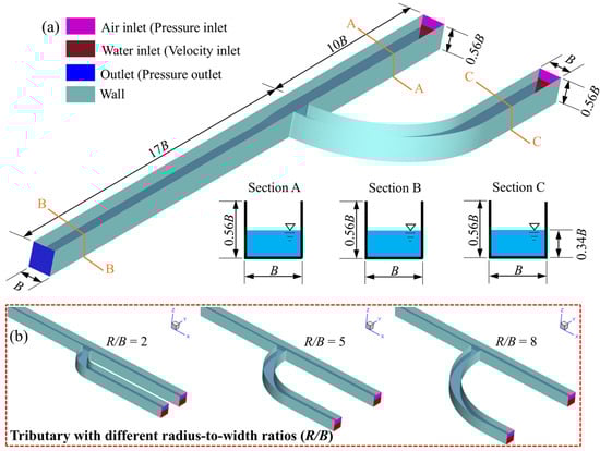
Figure 2.
(a) Model setup and boundary conditions. (b) Tributary with different radius-to-width ratios.
Figure 2b and Table 1 present the simulation case settings and the primary hydraulic parameters. We set three different radius-to-width ratios of the tributary (R/B) to study the effects on the hydrodynamic characteristics in the confluence. Furthermore, we added three values of q* ranging from 0.25 to 0.75 to study the effect of the flow ratio q* on the flow structure at the confluence. In the previous literature on confluence [23,24], the value of q* ranged from 0.25 to 0.97.

Table 1.
Numerical cases.
2.2. Simulation Strategy
2.2.1. Turbulence Model
The Renormalization Group (RNG) k-ε turbulence model proposed by Yakhot and Orzag (1986) [25] can effectively predict the flow characteristics in a curved channel and can accurately capture more flow lines in the confluence [26]; therefore, it was employed in this study. The governing equations were as follows:
Continuity equation:
Momentum equation:
Turbulent kinetic energy (k) equation:
Turbulent dissipation rate () equation:
with
where ρ and p are the corresponding density and pressure, respectively; t is the time; μ is the molecular viscosity coefficient; and are the velocity components in the and directions; i, j, k = 1, 2, 3; is the turbulence viscosity; is the turbulent Prandtl number of k; is the term that increases the turbulent kinetic energy generated by the flow gradient; and is the critical value used to determine whether the flow has entered the “high-strain-rate state”. In this study, , , , , and are empirical constants that takes values of 0.0845, 1.42, 1.68, 4.38, and 0.012 [27], respectively.
2.2.2. VOF Two-Phase Flow Model
In this study, the Volume of Fluid (VOF) method proposed by Hirt and Nichols (1981) [28] was employed to capture the characteristics of the water–air interface. The governing equation is as follows:
where aw is the volume fraction of water. Furthermore, the volume fractions of water–air should satisfy continuity:
where the volume fraction of water may correspond to three potential states: (1) the cell is completely filled with water, aw = 1.0; (2) the cell is fully occupied by air, aw = 0.0; and the (3) cell is located within an infinitesimally small region, 0 < aw < 1.
2.2.3. Methods and Boundary Conditions
The ANSYS FLUENT 2022 R1 software was employed for numerical simulation in this study. The CPU and RAM of the computing machine were Inter(R) Xeon(R) Platinum 8370 C @ 2.80 GHZ and 512 GB, respectively. The semi-implicit method for pressure-linked equations (SIMPLE) algorithm was selected to solve the pressure–velocity coupling equations, and the pressure interpolation scheme was PRESTO! Specifically, the first-order upwind scheme was applied to discretize the turbulent kinetic energy and turbulent dissipation rate, while the second-order upwind scheme was employed for the discretization of all other parameters.
As shown Figure 2a, the water and air phases were the velocity and pressure inlets, respectively, with both directions being perpendicular to the inlet section. The outlet boundary was the pressure outlet, the pressure value was determined by the water depth, and the wall boundary adopted the standard wall function method.
2.2.4. Mesh Generation and Testing
The ICEM CFD software 2022 R1 was selected to generate structured hexahedral grids. Considering the complex flow structure in the confluence, a more refined grid was used. In order to capture more flow details with increased accuracy, a finer grid was used for the water phase; furthermore, a 1 mm grid was used to obtain more information about the walls (Figure 3a). As shown in Figure 3b, three different simulation scenarios with different radius-to-width ratios adopted the same grid division method.
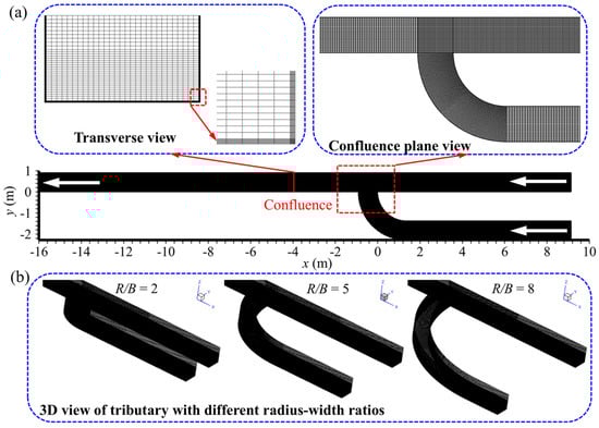
Figure 3.
(a) The mesh of the computational domain. (b) Three-dimensional meshes of the tributary with different radius-to-width ratios. The white arrow indicates the direction of flow.
The mesh size has a crucial impact on the simulation results. It is of note that the model used by Zhang et al. (2025) [1] is similar to the model in this study and can therefore provide a reference for the selection of the grid scale in this study, eliminating the need for unnecessary experimental calculations. The meshes with 492,660 (Mesh 1), 1,282,348 (Mesh 2), and 3,065,280 (Mesh 3) cells were divided to select the optimal computational grid. The combined velocity in the x and y directions (uxy) was used to verify the grid dependence, as this can better reflect the fluid dynamic characteristics of the flow direction. For ease of analysis, normalized coordinates were adopted as X = x/B. As shown in Figure 4, the value of uxy in Mesh 1 (492,660) was significantly lower than that of Mesh 2 and Mesh 3. The values of uxy aligned closely when the number of cells increased from 1,282,348 (Mesh 2) to 3,065,280 (Mesh 3), with a change rate of 0.32%. The fundamental reason for the differences in calculation results under different grids is that the grid size directly determines the “discretization accuracy”; therefore, considering the accuracy and computational efficiency of the simulation, Mesh 2 was chosen for this study.
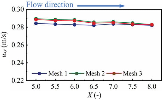
Figure 4.
Distribution of uxy at different sections in the confluence.
2.3. Model Validation
We selected the 90° equally wide confluence flume proposed by Weber et al. (2001) [19] for model validation, as it is from a classic study with reliable experimental data. The entire flume system was composed of a main channel and tributary, all with a width of 0.914 m (Figure 5). The lengths of the main channel and the tributary were 21.95 m and 3.66 m, respectively, while the model height and downstream water depth were 0.51 m and 0.296 m, respectively.
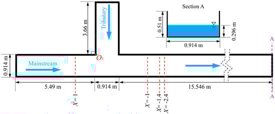
Figure 5.
Experimental layout from Weber et al. (2001) [19].
The flow ratio of the selected verification case was 0.25, while Qm and Qt were 0.042 m3/s and 0.127 m3/s, respectively. To facilitate comparison and analysis, both the experimental data and the numerical values have been normalized according to the following formula: X = x/B, Y = y/B, Z = z/B, where uxy represents the resultant velocity in the x and y directions.
Figure 6 shows the comparison of the numerical values (black circle) and the experimental data (red line). We selected the experimental data from the near-bed (Z = 0.014) and near-water surfaces (Z = 0.278) at three different planes (X = −2, −1.4, 1) for comparison. This numerical model successfully reproduced the velocity (uxy) distribution trend, and the calculated data were consistent with the experimental data.
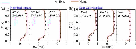
Figure 6.
Comparison of numerical values with experimental data by Weber et al. (2001) [19]. (a) Near bed surface (Z = 0.014). (b) Near water surface (Z = 0.278).
To obtain a more accurate assessment of the simulation results, a quantitative analysis was conducted. As shown in Table 2, the five key errors proposed by Blocken and Gualtieri (2012) [29] were selected, namely Root Mean Square Error (RMSE), Bias, Mean Square Error (MSE), Mean Absolute Error (MAE), and Mean Relative Error (MRE). A smaller absolute value of the error indicates that the difference between the numerical values and the experimental data is smaller. The statistical errors of the velocity distribution are presented in Table 2, where it can be observed that the values of the key errors are all relatively small.
Table 2.
Critical errors and results at different horizontal planes for uxy.
3. Results and Discussion
3.1. Longitudinal Velocity
3.1.1. Horizontal Flow Pattern
Figure 7 shows the different patterns of the flow near the bed surface (Z = 0.014) and water surface (Z = 0.278) in Case A1. The flow near the bed surface (Z = 0.014) enters the main channel at a larger flow angle and flows towards the outer bank of the main channel (the blue rectangle) (Figure 7a). Near the water surface (Z = 0.278), the tributary flows into the main channel at a smaller flow angle (Figure 7b), which is consistent with the findings of Weber et al. (2001) [19]. The smaller flow angle results in a smaller transverse kinetic energy near the water surface, which in turn leads to the SZ scale near the water surface being smaller than that near the bed surface, especially in terms of the length of the SZ. This is because the angle of the water flowing near the bed surface is larger, which results in an increased concentration of high flow velocities near the bed surface. Moreover, compared to near the water surface, a more noticeable flow stagnation phenomenon is observed near the bed plane where the tributary flow connects with the upstream section of the main channel.
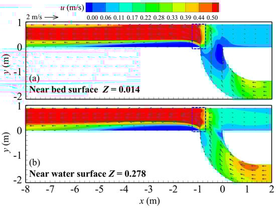
Figure 7.
The flow structures at different water depth positions (Case A1). (a) Z = 0.014, near bed surface; (b) Z = 0.278, near water surface.
3.1.2. Effect of Flow Ratio and Radius-to-Width Ratio on the Velocity Distribution
To further study the field structure downstream of the confluence, Figure 8 shows the longitudinal distribution of the normalized flow velocity u* under different radius-to-width ratios (R/B) and flow ratios (q*). Figure 8a–f illustrate the effect of R/B and q* on the velocity distribution, demonstrating that the scale of the recirculation zone (black rectangle) and the MVZ (purple rectangle) increase as R/B increases, and the water flow needs a longer distance to recover. Furthermore, the scale of the recirculation zone and MVZ decreases as q* increases (Figure 8d–f), and the distance for the water flow to recover shortens [1].
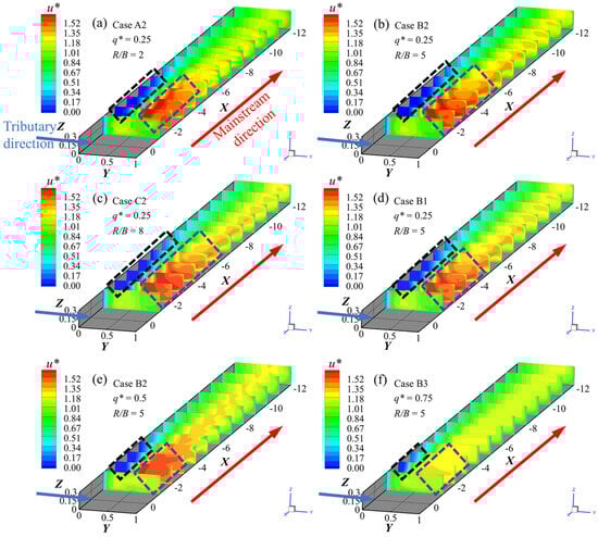
Figure 8.
The longitudinal distribution of u* downstream in the confluence with different R/B and q*. (a) Case A2. (b) Case B2. (c) Case C2. (d) Case B1. (e) Case B2. (f) Case B3. The black and purple rectangular boxes represent the recirculation zone and the MVZ, respectively.
3.2. Turbulent Kinetic Energy
Turbulent kinetic energy (TKE) represents the distribution of turbulence intensity in the flow field. Figure 9 shows the distribution of TKE with different cross-sections. The peak value of TKE occurs on the inner bank of the main channel (Figure 9a) in almost the same position as that of the SZ, then decreases for an increasing longitudinal distance, which indicates that turbulence decreases and the flow gradually recovers.
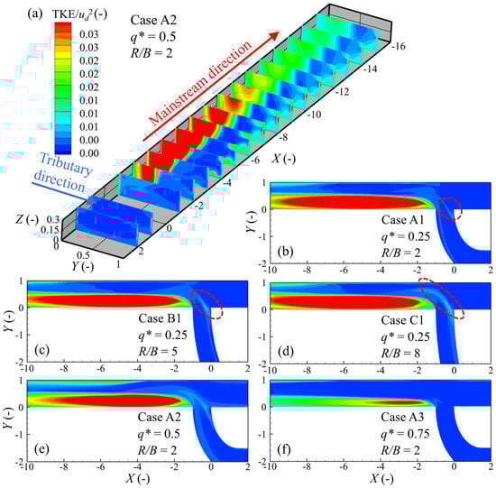
Figure 9.
Distribution of normalized turbulent kinetic energy in confluence. (a) Distribution of TKE at different cross-sections in Case A2. (b–d) Distribution of TKE at water surface plane (Z = 0.278) with different R/B. (b,e,f) Distribution of TKE at water surface plane with different q*. The red circles represent the distribution of TKE within the stagnant zone.
To further analyze the influence of R/B and q* on the distribution of TKE, Figure 9b–f show the distribution of TKE near the water surface (Z = 0.278, demonstrating that TKE downstream of the confluence remains almost unchanged as the R/B increases, while that upstream of the confluence increases as the R/B increases (red circle). This is mainly because the velocity on the inner side of the bend increases as the R/B increases, thereby forming a strong turbulent flow at the outlet of the tributary close to the upstream of the main channel. As shown in Figure 9b,e,f, the value of TKE decreases as q* increases; as the q* is large, the velocity of the tributary is much lower than that of the mainstream. Therefore, the lateral flow of the tributary will not cause significant interference to the flow field within the main channel.
3.3. Separation Zone
3.3.1. Characteristic Values of the Separation Zone
The SZ is an important feature downstream of the confluence, which is a low-velocity pressure recirculation structure [9]. Currently, many methods for identifying the SZ have been proposed; in previous studies, the zero-flow method, streamline method, contour method, and three-dimensional streamline method [30,31,32] were utilized. Jin et al. (2023) [30] systematically compared several methods and provided detailed descriptions of the SZ, the recirculation zone, and the countercurrent zone. In this study, the zero longitudinal velocity method proposed by Yang et al. (2009) [32] was adopted to identify the boundary of the SZ (Figure 10), as it has a higher physical accuracy. The maximum width of the SZ occurs at the middle water depth, consistent with the findings of Schindfessel et al. (2017) [31]. Unlike the straight confluent channel, the length of the SZ decreases as the water depth increases in this study, which might be caused by the different flow structures within the straight and curved tributaries. The differences in the tributary morphologies significantly affect the formation and evolution of the SF downstream of the confluence, thereby leading to changes in the scale of the SZ. The width (Ws) and length (Ls) of the SZ are defined as the maximum vertical distance from the boundary to the left bank and the length intercepted by the boundary of the SZ, respectively (Figure 10).
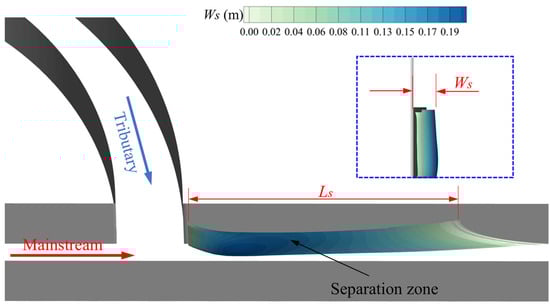
Figure 10.
Three-dimensional schematic diagram of SZ.
3.3.2. Variation in the Scale of the Separation Zone
As shown in Figure 11, the scale of the SZ varies with the changes in the R/B and the q*: it increases as R/B increases and decreases as q* increases (Figure 11a,b). To further investigate the effects of R/B and q* on the shape of the SZ, the aspect ratio Ws/Ls was used. A value of Ws/Ls closer to “1” implied that the shape of the SZ was “fuller”. Furthermore, three planes (Z = 0.06, 0.16, 0.3) were identified to study the effects of R/B and q* on the aspect ratio Ws/Ls. As shown in Figure 11c,d, although the values of Ws/Ls at the three positions are relatively close and the shape of the SZ tends to be flat, the peak value of Ws/Ls occurs at the middle water depth (Z = 0.16). This indicates that the shape of the SZ is “fuller” at Z = 0.16, at which point the value of Ws/Ls increases with the effect of q* (Figure 11c); conversely, the value of Ws/Ls decreases with the increase in R/B (Figure 11c).
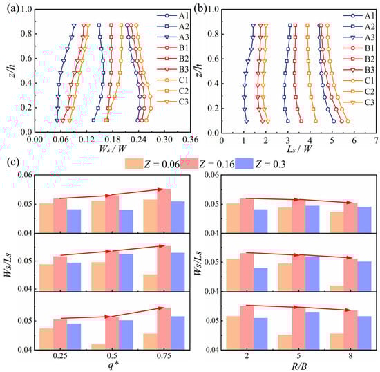
Figure 11.
(a) Variation in the width of the SZ under different q*and R/B. (b) Variation in the length of the SZ under different q*and R/B. (c) Variation in the aspect ratio of of the SZ under different q*and R/B.
3.4. Secondary Flow
3.4.1. Formation and Evolution of Secondary Flow
As one of the important features in the downstream of confluence, SF is formed because of centrifugal force and the lateral pressure gradient [10]. The scale and position of SF change as the longitudinal distance increases. Therefore, before studying the effects of R/B and q* on the SF, it is important to analyze its formation and evolution process.
The transverse velocity v and the vertical velocity w are important hydraulic parameters that reflect the movement patterns and intensities of SF. For Case A2, the distribution of uyz in different cross-sections is shown in Figure 12a, where it can be observed that the maximum value of uyz occurs near the confluence. The value of uyz decreases as the distance increases, indicating that the SF intensity gradually weakens.
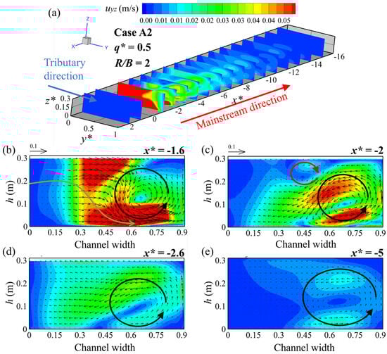
Figure 12.
(a) The longitudinal distribution of Uyz downstream of the confluence (Case A2). (b–e) The formation and evolution of SF (Case A2). The circles and the green curves represent the secondary flow and the flow direction. x* = x/W.
Figure 12b–e depict the evolution of SF in cross-sections X = −1.6 to −5. In the section X = −1.6, SF is observed in a clockwise direction (Figure 12b). The lateral flow from the inner to the outer bank occupies most of the cross-section, and as the longitudinal distance increases, only the counterclockwise SF is observed at X = −2.6, while the clockwise SF disappears. The main reason is that as the distance increases, uyz decreases, the flow gradually returns to normal, and the smaller SF structures disappear [2]. The peak value of uyz with a smaller magnitude occurs on the right side of the X = −5 cross-section.
3.4.2. Effect of Radius-to-Width Ratios and Flow Ratios on the Evolution of Secondary Flow
Figure 13a–c show the distribution of SFs in the downstream of the confluence with different R/B (2, 5, and 8) when q* = 0.75. The peak value of uyz decreases as the longitudinal distance increases, and gradually moves towards the right bank of the section. Furthermore, the scale of the SF gradually increases as the distance increases. A smaller scale SF in the counterclockwise direction is observed at the position close to the bed on the X = −3 section (Figure 13a). As the R/B increases, the uyz value decreases at the X = −3 cross-section and the scale of the SF decreases. Even at R/B = 8 (Case C3), no SF is observed within this section. At the cross-sections X = −7 and X = −11, the value of uyz and the scale of the SF decrease as R/B increases, because as the R/B increases, the disturbance in the mainstream tributary flow decreases, thereby exerting an inhibitory effect on the formation of the SF.
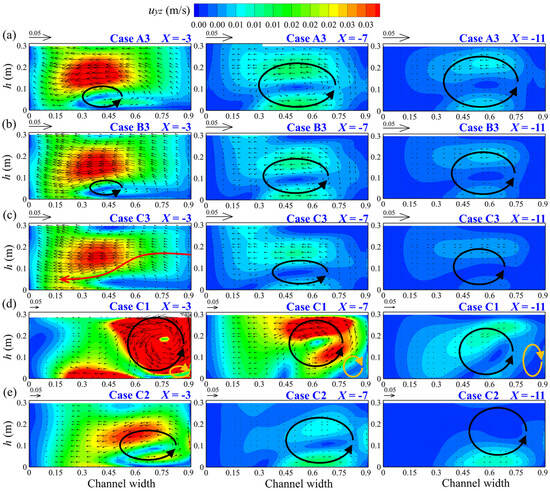
Figure 13.
Evolution of SF with different q* and R/B. (a,b) Effect of R/B on the evolution of SF. (c–e) Effect of q* on the evolution of SF.
Figure 13c–e show the distribution of SFs in the downstream cross-section of the confluence when R/B = 8 with different q* (0.25, 0.5, and 0.75). As shown in Figure 13d, the maximum value of uyz is located closely to the right side of the section, and an SF with a larger scale in the counterclockwise direction and a smaller size in the clockwise direction (Case C1) is observed on the right bank. As q* increases, the SF in the clockwise direction disappears and the scale of the SF in the counterclockwise direction decreases (Case C2). Furthermore, as q* increases, the number of SFs within the cross-section decreases and the scale of the SFs also reduces because of the influence of the tributary flow on the mainstream and the turbulence intensity as q* increases. However, the formation of SF requires specific hydraulic conditions, which leads to the inhibition of the formation and development of SF.
3.4.3. Quantification of Secondary Flow Intensity
The large lateral flow of a tributary is a notable feature of the confluence section. The current criterion for evaluating the SF intensity is based mainly on the combination of v–w, which would lead to an overestimation of the SF intensity at the confluence, even if no obvious SF phenomenon was actually observed [30]. Therefore, to further reasonably evaluate the distribution of SF intensity in the confluent channel, a new evaluation criterion was proposed in this study. Considering that the vertical velocity w and longitudinal velocity u are important hydraulic parameters representing the SF motion pattern and the flow characteristics in the confluence, respectively, the evaluation criteria are as follows:
where represents the secondary flow intensity; and u, w, and A represent the longitudinal velocity, vertical velocity, and the cross-section area, respectively.
Figure 14 illustrates the distribution of the mean SF intensity at different cross-sections with different R/B and q*. shows a trend of gradually increasing and then decreasing, with the peak value of occurring at the downstream section of the confluence, consistent with the findings of Shen et al. (2022) [26]. Furthermore, R/B and q* have almost no effect on the SF intensity in the upstream of the confluence. The peak value of increases with the increase in R/B and decreases with the increase in q*, mainly because the influence of the curved boundary on the water flow in the tributary decreases as the R/B increases. This results in a stronger lateral flow of the tributary, which in turn creates more favorable conditions for the formation of SFs. Conversely, the squeezing effect of the mainstream on the tributary flow increases as q* enhances, and thus suppresses the development of SF.
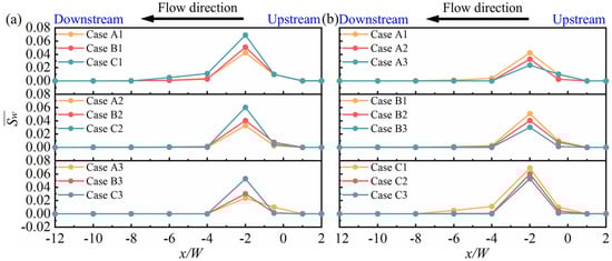
Figure 14.
Distribution of the in the confluence. (a) The influence of R/B on the . (b) The influence of q* on the .
4. Conclusions
In this study, we employed the RNG k-ε turbulence model to investigate the effects of the radius-to-width ratio of a tributary (R/B) and the flow ratio (q*) on the hydrodynamic characteristics of the confluence. Specifically, the obtained results were as follows:
- 1.
- The patterns of flow are different near the surface and near the bottom. Near the surface, the tributary water flows into the main channel and moves significantly towards the outer bank of the main channel; conversely, at near the bottom surface, the tributary water flows towards the downstream direction.
- 2.
- The MVZ and scale of the SZ increase as the R/B increases. The peak value of Ws/Ls occurs at the middle water depth and increases with the increase in the R/B; conversely, the MVZ and the scale of the SZ decrease as the q* increases and the value of Ws/Ls decreases as the q* increases.
- 3.
- The peak value of TKE is always located on the left bank of the main channel. The TKE value in the upstream of the confluence increases as the R/B increases, while there is almost no change downstream. Moreover, the value of TKE decreases as the q* increases.
- 4.
- The scale of SF decreases as R/B and q* increase and the peak value of the always occurs downstream of the confluence. Notably, the value of the increases and decreases as the R/B and q* increase.
While this study was centered on the effect of R/B on the hydrodynamic characteristics of the confluence, it lacked an in-depth investigation into factors like wall roughness and bed morphology. Accordingly, future research ought to incorporate the impacts of these factors for more comprehensive analysis.
Author Contributions
Conceptualization, Y.Z. and H.Y.; methodology, H.T.; software, L.Y.; validation, H.T. and R.H.; formal analysis, H.Y.; investigation, Y.Z. and H.T.; resources, L.Y.; data curation, R.H.; writing—original draft preparation, Y.Z.; writing—review and editing, H.T.; visualization, R.H. and H.Y.; supervision, H.Y.; project administration, R.H.; funding acquisition, R.H. and H.Y. All authors have read and agreed to the published version of the manuscript.
Funding
This research was funded by the National Natural Science Foundation of China (Grant No. 52479059), the science and technology research program of Chongqing Education Commission of China (Grant No. KJQN202400705), the public announcement and appointment program of the Chongqing Xike Water Transport Engineering Consulting Co., Ltd. (Grant No. 2024990007), Chongqing Water Conservancy Science and Technology Project (Grant No. CQSLK-2023018), and Chongqing Natural Science Foundation General Program (Grant No. CSTB2024NSCQ-MSX0824), and The APC was funded by the National Natural Science Foundation of China (Grant No. 52479059).
Data Availability Statement
Dataset available on request from the authors.
Acknowledgments
We are grateful to ZongJiang Zhang of Chongqing Jiaotong University, China, for the data processing and discussion. We would like to express our gratitude to the Editor, Associate Editor, and all anonymous reviewers for their valuable feedback and insightful comments.
Conflicts of Interest
The authors declare that this study received funding from Chongqing Xike Water Transport Engineering Consulting Co., Ltd. The funder had the following involvement with the study: investigation and visualization.
References
- Zhang, J.; Miao, M.; Wang, W.; Li, Z.; Li, P.; Wang, H.; Wu, Z.; Zhao, B.; Li, J. Three-Dimensional Flow Characteristics and Structures in Confluences Based on Large Eddy Simulation. J. Hydrol. 2025, 655, 132956. [Google Scholar] [CrossRef]
- Shen, X.; Li, S.; Cai, H.; Wang, K.; Yuan, X.; Li, D.; Li, P. The Response Mechanism of Transversal Mixing of Dissolved Oxygen to the Evolution of SF at the Confluence. J. Hydrol. 2024, 635, 131184. [Google Scholar] [CrossRef]
- Shi, X.; Jin, Q.; Chen, H.; Tao, H.; Song, T. Analysis of Pollutant Diffusion Characteristics with Intersection Angle of 45° in Environmental Open Channel. Int. J. Environ. Sci. Technol. 2024, 22, 5543–5554. [Google Scholar] [CrossRef]
- Canelas, O.B.; Ferreira, R.M.L.; Cardoso, A.H. Hydro-morphodynamics of an Open-channel Confluence with Bed Discordance at Dynamic Equilibrium. Water Resour. Res. 2022, 58, e2021WR029631. [Google Scholar] [CrossRef]
- Yuan, S.; Xu, L.; Tang, H.; Xiao, Y.; Gualtieri, C. The Dynamics of River Confluences and Their Effects on the Ecology of Aquatic Environment: A Review. J. Hydrodyn. Ser. B (Engl. Ed.) 2022, 34, 1–14. [Google Scholar] [CrossRef]
- Yuan, S.; Zheng, Y.; Tang, H.; Chen, Y.; Xu, L.; Whittaker, C.; Gualtieri, C. Large Wood Transport and Accumulation near the SZ of a Channel Confluence. Water Resour. Res. 2024, 60, e2023WR034790. [Google Scholar] [CrossRef]
- Cao, L.; Shen, X.; Cai, H.; Gao, W.; Li, S.; Li, D. Mechanisms of Influence of Confluence Containing Spur-Dike on Microplastic Transport and Fate. J. Hydrol. 2024, 641, 131720. [Google Scholar] [CrossRef]
- Tang, H.; Zhang, H.; Yuan, S. Hydrodynamics and Contaminant Transport on a Degraded Bed at a 90-Degree Channel Confluence. Environ. Fluid Mech. 2018, 18, 443–463. [Google Scholar] [CrossRef]
- Best, J.L.; Reid, I. Separation Zone at Open-channel Junctions. J. Hydraul. Eng. 1984, 110, 1588–1594. [Google Scholar] [CrossRef]
- Bradbrook, K.F.; Lane, S.N.; Richards, K.S.; Biron, P.M.; Roy, A.G. Role of Bed Discordance at Asymmetrical River Confluences. J. Hydraul. Eng. 2001, 127, 351–368. [Google Scholar] [CrossRef]
- Gurram, S.K.; Karki, K.S.; Hager, W.H. Subcritical Junction Flow. J. Hydraul. Eng. 1997, 123, 447–455. [Google Scholar] [CrossRef]
- Constantinescu, G.; Koken, M.; Zeng, J. The Structure of Turbulent Flow in an Open Channel Bend of Strong Curvature with Deformed Bed: Insight Provided by Detached Eddy Simulation. Water Resour. Res. 2011, 47, W05515. [Google Scholar] [CrossRef]
- Penna, N.; De Marchis, M.; Canelas, O.; Napoli, E.; Cardoso, A.; Gaudio, R. Effect of the Junction Angle on Turbulent Flow at a Hydraulic Confluence. Water 2018, 10, 469. [Google Scholar] [CrossRef]
- Demir, V.; Keskin, A.Ü. Obtaining the Manning Roughness with Terrestrialremote Sensing Technique and Flood Modeling Using FLO-2D: A Case Study Samsun from Turkey. Geofizika 2020, 37, 131–156. [Google Scholar] [CrossRef]
- Shen, X.; Li, D.; Cao, L.; Wang, K.; Yuan, X.; Li, X.; Li, S. The Influence of Vortex Flow Generated by Spur Dikes on the Distribution and Mixing of Dissolved Oxygen at a Wide-Shallow Confluence. Phys. Fluids 2024, 36, 105106. [Google Scholar] [CrossRef]
- He, X.; Yu, M.; Wang, K.; Liu, Y. Propagation of the Effect of Upstream Bend Circulations to Downstream Flow and Sediment Transport in Consecutive River Bends. J. Hydrol. 2025, 660, 133358. [Google Scholar] [CrossRef]
- Pan, Y.; Liu, X.; Yang, K. Effects of Discharge on the Velocity Distribution and Riverbed Evolution in a Meandering Channel. J. Hydrol. 2022, 607, 127539. [Google Scholar] [CrossRef]
- Hu, R.; Zhang, J. Numerical Study on the Outer Bank Cell of SF in a U-Shaped Open Channel. KSCE J. Civ. Eng. 2023, 27, 1558–1567. [Google Scholar] [CrossRef]
- Weber, L.J.; Schumate, E.D.; Mawer, N. Experiments on Flow at a 90° Open-Channel Junction. J. Hydraul. Eng. 2001, 127, 340–350. [Google Scholar] [CrossRef]
- Shumate, E.D. Experimental Description of Flow at an Open-Channel Junction. Master thesis, University of Iowa, Iowa City, IA, USA, 1998. [Google Scholar]
- Wei, L.; Li, W.; Pan, Y.; Li, K.; Yang, K. SF Characteristics in Confluent Streams with Vegetation. J. Hydrol. 2024, 640, 131722. [Google Scholar] [CrossRef]
- Hu, C.; Yu, M.; Wei, H.; Liu, C. The Mechanisms of Energy Transformation in Sharp Open-Channel Bends: Analysis Based on Experiments in a Laboratory Flume. J. Hydrol. 2019, 571, 723–739. [Google Scholar] [CrossRef]
- Boyer, C.; Roy, A.G.; Best, J.L. Dynamics of a River Channel Confluence with Discordant Beds: Flow Turbulence, Bed Load Sediment Transport, and Bed Morphology. J. Geophys. Res. 2006, 111, F04007. [Google Scholar] [CrossRef]
- Yuan, S.; Tang, H.; Xiao, Y.; Qiu, X.; Zhang, H.; Yu, D. Turbulent Flow Structure at a 90-Degree Open Channel Confluence: Accounting for the Distortion of the Shear Layer. J. Hydro-Environ. Res. 2016, 12, 130–147. [Google Scholar] [CrossRef]
- Yakhot, V.; Orszag, S.A. Renormalization Group Analysis of Turbulence. I. Basic Theory. J. Sci. Comput. 1986, 1, 3–51. [Google Scholar] [CrossRef]
- Shen, X.; Li, R.; Cai, H.; Feng, J.; Wan, H. Characteristics of SF and SZ with Different Junction Angle and Flow Ratio at River Confluences. J. Hydrol. 2022, 614, 128537. [Google Scholar] [CrossRef]
- Han, Z.; Reitz, R.D. Turbulence Modeling of Internal Combustion Engines Using RNG κ-ε Models. Combust. Sci. Technol. 1995, 106, 267–295. [Google Scholar] [CrossRef]
- Hirt, C.W.; Nichols, B.D. Volume of Fluid (VOF) Method for the Dynamics of Free Boundaries. J. Comput. Phys. 1981, 39, 201–225. [Google Scholar] [CrossRef]
- Blocken, B.; Gualtieri, C. Ten Iterative Steps for Model Development and Evaluation Applied to Computational Fluid Dynamics for Environmental Fluid Mechanics. Environ. Model. Softw. 2012, 33, 1–22. [Google Scholar] [CrossRef]
- Jin, T.; Ramos, P.X.; Mignot, E.; Riviere, N.; De Mulder, T. On the Delineation of the Flow SZ in Open-Channel Confluences. Adv. Water Resour. 2023, 180, 104525. [Google Scholar] [CrossRef]
- Schindfessel, L.; Creëlle, S.; De Mulder, T. How Different Cross-Sectional Shapes Influence the SZ of an Open-Channel Confluence. J. Hydraul. Eng. 2017, 143, 4017036. [Google Scholar] [CrossRef]
- Yang, Q.-Y.; Wang, X.-Y.; Lu, W.-Z.; Wang, X.-K. Experimental Study on Characteristics of SZ in Confluence Zones in Rivers. J. Hydrol. Eng. 2009, 14, 166–171. [Google Scholar] [CrossRef]
Disclaimer/Publisher’s Note: The statements, opinions and data contained in all publications are solely those of the individual author(s) and contributor(s) and not of MDPI and/or the editor(s). MDPI and/or the editor(s) disclaim responsibility for any injury to people or property resulting from any ideas, methods, instructions or products referred to in the content. |
© 2025 by the authors. Licensee MDPI, Basel, Switzerland. This article is an open access article distributed under the terms and conditions of the Creative Commons Attribution (CC BY) license (https://creativecommons.org/licenses/by/4.0/).