Analysis of Greenhouse Gas Emissions from China’s Freshwater Aquaculture Industry Based on the LMDI and Tapio Decoupling Models

Abstract

Carbon emissions from freshwater aquaculture can exacerbate the greenhouse effect, thereby impacting human life and health. Consequently, it is of great significance to explore the carbon peak process and the role of emission reduction data in China’s freshwater aquaculture industry. This study innovatively employs the Logarithmic Mean Divisia Index model (LMDI) and the Tapio decoupling model to conduct an in-depth analysis of the relationship between carbon emissions and output values in the freshwater aquaculture industry, accurately identifying the main driving factors. Meanwhile, the global and local Moran’s I indices are introduced to analyze its spatial correlation from a new perspective. The results indicate that from 2013 to 2023, carbon emissions from China’s freshwater aquaculture industry exhibited a quasi-“N”-shaped trend, reaching a peak of 38 million tons in 2015. East China was the primary contributor to carbon emissions, accounting for 46%, while South China, Central China, and Northeast China each had an average annual share of around 14%, with Southwest, North China, and Northwest China contributing relatively small proportions. The global Moran’s I index showed a decreasing trend, with a p-value ≤ 0.0010 and a z-score > 3.3, indicating a 99% significant spatial correlation. High-high clusters were concentrated in some provinces of East China, while low-low clusters were found in Northwest, North, and Southwest China. The level of fishery economic development positively drove carbon emissions, whereas freshwater aquaculture production efficiency, industrial structure, and the scale of the aquaculture population had negative effects on carbon emissions. During the study period, carbon emissions exhibited three states: weak decoupling, strong decoupling, and expansive negative decoupling, with alternating strong and weak decoupling occurring after 2015.

1. Introduction

Greenhouse gas emissions are the underlying cause of environmental issues, including global warming, sea-level rise, and the increasing frequency of extreme weather events. It is estimated that future global CO₂ emissions could lead to a rise in Earth’s temperature by 1.5–2 °C [1], posing a severe threat to human survival and development [2]. To alleviate the global food security crisis and address human needs, there has been an increasing demand for aquatic products such as fish and shrimp, which are rich in high-quality animal protein. This has subsequently led to the rapid development of the aquaculture industry [3,4]. It is projected that the global scale of aquaculture will expand rapidly by 200% by 2050 [5,6], and the substantial greenhouse gas emissions generated from this sector are exacerbating the trend of global warming [4]. In 2020, the global aquaculture production reached a staggering 120 million tons, with freshwater aquaculture contributing approximately 54 million tons to this total [7]. The emissions from freshwater aquaculture exhibit significant variability both spatially and temporally [8,9,10], with fluctuations reaching up to threefold. This high degree of uncertainty is particularly concerning. Consequently, there is an urgent need to reduce greenhouse gas emissions from the freshwater aquaculture sector and transition towards a low-carbon economic development model in this industry.

Nitrous oxide (N₂O), carbon dioxide (CO₂), and methane (CH₄) are all generated throughout the entire process of freshwater aquaculture. In the early stages, due to extensive input methods and an irrational industrial structure, the low-carbon development of aquaculture encountered bottlenecks. Compared to natural water bodies, the freshwater aquaculture industry is regarded as a high-intensity source of greenhouse gas emissions [11]. Furthermore, the anthropogenic greenhouse gases emitted from activities such as freshwater aquaculture can trigger severe issues such as climate change and ocean acidification [12], posing significant challenges to national aquaculture programs. Despite the growing recognition that freshwater aquaculture is a major source of CH₄, N₂O, and CO₂ emissions, the scale and dynamics of these emissions remain notably absent or inadequately specified in the assessment reports of the Intergovernmental Panel on Climate Change (IPCC), as well as in most global and regional greenhouse gas budgets [8,9,10,13,14]. Consequently, some scholars have initiated research on carbon emissions from the freshwater aquaculture industry to address this gap and contribute to the low-carbon development of the sector.

Methane emissions during the aquaculture process are influenced by a multitude of environmental factors, including weather conditions, hydrothermal regimes, nutrient content, and various other aspects [15]. Under anaerobic conditions, in water bodies rich in microorganisms, methane gas is produced through the degradation of organic matter. This methane is then released into the atmosphere via processes such as ebullition (gas bubbling), molecular diffusion, or plant-mediated transport [16,17]. Meanwhile, aquaculture systems receive substantial inputs of nutrients to accelerate primary production [18,19]. These nutrient inputs can interfere with microbial processes, subsequently influencing carbon emission dynamics [20]. Numerous studies have been conducted on the carbon emission processes and mechanisms associated with freshwater aquaculture. These studies, categorized based on the types of surface water bodies, encompass a variety of settings such as lakes, rivers, ditches, ponds, and reservoirs [21]. Carbon emissions from freshwater aquaculture encompass both direct and indirect emission processes [22]. Among these, direct carbon emission processes refer to the carbon emissions occurring during the production process of aquaculture, primarily including those resulting from energy consumption and nutrient cycling [23,24]. Indirect carbon emissions, on the other hand, refer to the carbon emissions generated during the production or manufacturing of various input factors for aquaculture. These primarily include emissions resulting from the construction of equipment such as fishing vessels and emissions associated with electricity consumption for facilities during the power generation process [25].

China ranks first in aquaculture production, accounting for nearly two-thirds of the global output [26,27,28]. Although China’s aquaculture systems can be divided into two major categories, namely marine aquaculture and freshwater aquaculture, existing research on carbon emissions has predominantly focused on the marine aquaculture sector, with relatively insufficient attention given to freshwater aquaculture. Specifically, most current research on carbon emissions in freshwater aquaculture centers on the aquaculture pond segment, while systematic studies on greenhouse gas emissions generated from resource consumption throughout the entire freshwater aquaculture process remain scarce [3,29]. There is a limited amount of literature in China examining the green development level and efficiency of the freshwater aquaculture industry, and existing research still has shortcomings. These are manifested as follows: firstly, the research perspectives are relatively narrow, lacking the establishment of a model evaluation system; secondly, a spatial analysis of emissions has not been conducted; thirdly, research is mostly based on a micro level, selecting locations such as villages, towns, and aquaculture farms, with a lack of studies at the provincial and national levels. In particular, research on freshwater aquaculture in western China is insufficient, necessitating supplementary and improved studies to formulate more targeted and comprehensive countermeasures and suggestions.

Based on this, this study focuses on carbon emissions from the freshwater aquaculture industry. By categorizing the emissions based on three greenhouse gases—methane (CH₄) and nitrous oxide (N₂O) generated through nutrient cycling, as well as carbon dioxide (CO₂) emitted from the combustion of diesel fuel in fishing vessels—this research conducts an in-depth analysis of carbon output and the potential for emission reduction in the freshwater aquaculture sector. Concurrently, this study employs the Logarithmic Mean Divisia Index (LMDI) model and the Tapio decoupling model to measure and analyze carbon emissions in China’s freshwater aquaculture industry. Furthermore, it introduces Moran’s I index to conduct a spatial correlation analysis of carbon emissions in this sector. Based on these analyses, targeted emission-reduction recommendations are proposed, thereby providing a theoretical foundation for mitigating climate change impacts in China’s freshwater aquaculture industry.

2. Methodology and Data

2.1. Study Area and Data Sources

The study area of this paper encompasses 31 provinces (autonomous regions, and municipalities directly under the central government) in China, excluding Hong Kong, Macao, and Taiwan due to data limitations. The study area is divided into eight major regions. The data utilized in this paper are sourced from the “China Fishery Statistical Yearbook” (2014–2023) [30] and the “China Statistical Yearbook” (2014–2023) [31], including data on freshwater aquaculture area, total power of fishing vessels, power of inland motorized fishing vessels, total power of motorized fishing vessels, output value of fishing vessel and machinery repair and manufacturing, total output value of freshwater aquaculture, total output value of fishery, number of the fishery population, and number of the fishery farming population. The energy consumption conversion coefficients for carbon emissions are derived from the “China Energy Statistical Yearbook,” [32] while some data are obtained from relevant research literature.

2.2. Methodology for Calculating Carbon Emissions in Freshwater Aquaculture

Carbon emissions from freshwater aquaculture primarily refer to the emissions of three greenhouse gases: methane (CH₄) and nitrous oxide (N₂O) generated through nutrient cycling within the aquaculture system itself, as well as carbon dioxide (CO₂) emitted from the combustion of diesel fuel in fishing vessels used for aquaculture [33]. These emissions are categorized into direct and indirect emissions. Among these, N₂O emissions are primarily influenced by feed inputs. However, due to the current lack of detailed data on feed inputs in fisheries statistics, coupled with the fact that N₂O emissions only account for approximately 1% of the total emissions of the three greenhouse gases [22], this study primarily focuses on CH₄ and CO₂ emissions.

Direct emissions:

(1)

Accounting for methane emissions

Methane is one of the primary greenhouse gases emitted from freshwater aquaculture systems. When dissolved oxygen levels in the water decrease, various organic matters, under the influence of methanogenic bacteria, tend to produce methane. Excess feed, fish excreta, and other organic matter increase the content of dissolved organic carbon in the water body, thereby providing more substrates for methanogenic bacteria. Referring to the research findings of Ma [24], the accounting method for methane emissions in this study is presented in Equation (1) as follows:

$$Q_{{CH}_4}=S_r\times {\mathrm{\rho }}_c$$

(1)

In the equation, Q_CH4 is the methane emissions, S_r is the area of freshwater aquaculture, and ρ_c is the methane emission coefficient per unit area of aquaculture.

(2)

Accounting for carbon dioxide emissions resulting from the use of diesel fuel in fishing vessels.

During the operation of fishing vessels, the combustion of diesel fuel emits a significant amount of carbon dioxide. The accounting for carbon dioxide emissions resulting from the use of diesel fuel in fishing vessels is presented in Equation (2) as follows:

$$Q_y=P\times \alpha \times \delta$$

(2)

In the equation, Q_y is CO₂ emissions generated from the diesel fuel consumed by the fishing vessel, P denotes the power of the fishing vessel (kW), α is the fuel consumption coefficient of the fishing vessel, and δ is the CO₂ conversion factor for diesel fuel.

To enable a unified measurement of emissions generated by different gases, this study converts the greenhouse effects of all gases into equivalent CO₂ emissions; the details are presented in Equation (3) as follows:

$$Q_c={\sum }_{i=1}^2{GHG}_i\times {GWP}_i$$

(3)

In the Equation, Q_c is the total CO₂ emissions under a unified standard; GHG_i is the emissions of two greenhouse gases, namely methane (CH₄) and carbon dioxide (CO₂); GWP_i is the global warming potential (GWP) values for different greenhouse gases, and according to the data on global warming potential (GWP) values published in the 2014 report by the Intergovernmental Panel on Climate Change (IPCC) [34], the GWP values for CH₄ and CO₂ are 28 and 1, respectively.

Indirect emissions:

This paper primarily considers carbon emissions arising from the construction of newly built vessels and the electricity consumption of various equipment.

(1)

The calculation of CO₂ emissions generated from the electricity consumption of newly added vessels is presented in Equation (4), as follows:

$$Q_a=Q_b\times {\rho }_b\times \mu$$

(4)

In the equation, Q_a is the CO₂ emissions generated from the construction of new vessels for freshwater aquaculture, Q_b is the output value of vessel construction for freshwater aquaculture, ρ_b is the electricity consumption coefficient for the output value of vessel construction, and μ is the carbon emission conversion coefficient for electricity consumption. Due to the lack of statistical data on the output value of vessel construction for freshwater aquaculture, this paper refers to the study by Wu Daqing [33] for estimation, as shown in Equation (5).

$$Q_b={\displaystyle \frac{P_b}{P_t}}\times Q_t$$

(5)

In the equation, P_b is the power (kW) of inland motorized fishing vessels; in the equation; P_t denotes the total power (kW) of motorized fishing vessels and Q_t is the output value (in ten thousand yuan) of the repair and manufacturing of fishing vessels and related machinery

(2)

Carbon dioxide emissions resulting from electricity consumption by water pumps

Water pumps are utilized for the make-up water supply in the process of freshwater aquaculture. The carbon dioxide emissions resulting from the electricity consumption of water pumps are calculated by drawing on the research of Xu [35], as detailed in Equation (6).

$$Q_s={\displaystyle \frac{Q_h}{{\lambda }_1}}\times \mu$$

(6)

$$Q_h=\left(1+200\times 2\%\right)\times S_r\times 1.5$$

(7)

In the Equation, the electricity consumption of the water pump is estimated based on the water exchange volume in aquaculture, and Q_s is the carbon dioxide emissions generated from the electricity consumption of the water pump. Assuming an average aquaculture water depth of 1.5 m, a water replenishment rate of 2%, and the water pump operating for 200 days a year, the approximate value of the water exchange volume in freshwater aquaculture is as shown in Equation (7), S_r is the area of freshwater aquaculture, λ₁ is the electricity consumption coefficient per unit volume of water used, and μ is the carbon emission conversion coefficient for electricity consumption

(3)

Carbon dioxide emissions resulting from electricity consumption by aeration equipment

Aeration equipment is primarily employed to regulate water quality in freshwater aquaculture and is widely utilized during the aquaculture process. This paper refers to the research conducted by Li [36] and calculates the carbon dioxide emissions resulting from electricity consumption by this equipment based on its operational duration, as detailed in Equation (8):

$$Q_z=N_z\times T\times {\lambda }_2\times \mu$$

(8)

$$N_z=S_r\times 15\times 80\mathrm{\%}\times {\displaystyle \frac{0.15}{3}}$$

(9)

In the Equation, Q_z is the carbon dioxide emissions generated from the electricity consumption by the aerator, and N_z is the number of aerators. According to the research conducted by Xu Hao [35], it is hypothesized that 80% of the aquaculture area requires aeration machines. Each hectare consumes 2.25 kilowatts of power, and the power rating of a single aeration machine is 3 kW. Consequently, the number of aeration machines can be calculated using Equation (9); S_r is the area of freshwater aquaculture, and T is the operating time of an aerator. Suppose one aerator operates for 4 h per day and works for 200 days each year, λ₂ is the power consumption coefficient per unit time of the aerator, and μ is the carbon emission conversion coefficient for electricity consumption.

(4)

Calculation of carbon dioxide emissions resulting from electricity consumption by feeders

Feeders can not only reduce labor costs but also improve feed utilization efficiency. This paper similarly calculates the carbon dioxide emissions resulting from electricity consumption based on the operating time of this equipment, as demonstrated in Equation (10):

$$Q_t=N_t\times T\times {\lambda }_3\times \mu$$

(10)

$$N_t={\displaystyle \frac{S_r}{0.8}}$$

(11)

Q_t is the carbon emissions generated from the electricity consumption by the feeder, and T is the operating time of the bait feeder. It is typically used 4 to 5 times per day, with each session lasting 0.5 h, and it operates for 200 days a year [37]. N is the number of bait feeders, and each bait feeder covers an area ranging from 0.6 to 1.0 hectares [36]. S_r is the area of freshwater aquaculture, λ₃ is the power consumption coefficient of the bait feeder, and μ is the carbon emission conversion coefficient. The parameter values involved in the carbon emission calculation in this paper are referenced from Wu [33], as shown in

Table 1. Parameter index description.

Index	Parameter	Reference
Fishing vessel construction (ρb)	100~300 kW·h/104 yuan	[35]
Water pump (λ1)	60 m3/kW·h
Oxygenator (λ2)	3~3.79 kW	[36,38]
Feeder (λ3)	0.075 kW	[22]
Fishing vessel fuel consumption (α)	0.225 t/kW	Reference Standards for Calculating the Fuel Consumption for Domestic Motorized Fishing Vessels’ Oil Subsidy
Nitromethane (ρc)	51.60 kg/hm2	[24]
Diesel (δ)	3.21 kg CO2/kg	[39]
electrical power (μ)	0.78 kg CO2/kW·h	[40]

.

2.3. Spatial Autocorrelation Analysis Using Moran’s I Index

Global spatial autocorrelation can be used to measure the spatial correlation of carbon emissions among different regions in the country. It is commonly represented by Moran’s I index, which ranges from −1 to 1. If Moran’s I is positive, it indicates the significant spatial clustering of regions, whereas a negative Moran’ I suggests a notably dispersed spatial pattern among regions [41,42], as detailed in Equation (12).

$$I={\displaystyle \frac{\sum _{i=1}^n\sum _{j=1}^n{W}_{ij}\left(x_i-\overline{x}\right)\left(x_j-\overline{x}\right)}{S^2\sum _{i=1}^n\sum _{j=1}^n{W}_{ij}}}$$

(12)

In Equation (12), n is the number of observations, S² is the variance of the observations, $\overline{x}$ is the mean of the observations, W_ij is the spatial weight matrix, and x_i and x_j respectively represent the carbon emission levels of freshwater aquaculture in the i-th and j-th regions of the spatial unit.

Both “High-High” and “Low-Low” are classified as hotspot areas. “High-High” indicates that high-value regions are surrounded by high-value neighbors, forming a “high-value cluster,” while “Low-Low” denotes that low-value regions are encompassed by low-value neighbors, creating a “low-value cluster.” In contrast, “High-Low” and “Low-High” are identified as outlier areas. “High-Low” represents a scenario where high-value regions are adjacent to low-value neighbors, resulting in a “spatial outlier,” and “Low-High” describes a situation where low-value regions are surrounded by high-value neighbors, also forming a “spatial outlier.”

We employed ArcGIS software (ArcMap 10.8.1) to process the administrative division data of the study area. Specifically, we imported and organized the administrative boundary data of various regions (provinces, autonomous regions, and municipalities directly under the central government) in China, ensuring the accuracy and completeness of the data. By utilizing the Moran’s I spatial analysis function in Arcgis, we can visually identify the adjacency relationships among different regions and export this adjacency information into tabular or other appropriate data formats, thereby providing foundational data support for the subsequent construction of a spatial weight matrix. We opted for the Queen contiguity method because it considers all provinces as adjacent if they share a common boundary or vertex. This method offers a more comprehensive reflection of inter-provincial spatial relationships and helps avoid overlooking potential spatial interactions.

2.4. Factors Influencing Freshwater Agricultural Carbon Emissions and Decomposition Models

Index decomposition analysis (IDA) has been extensively utilized to better investigate the trends in the driving factors of CO₂ emissions and energy consumption [43]. Since there are no residual variables in the Divisia index method, it has become the predominant empirical research method in the research field. Moreover, the Logarithmic Mean Divisia Index (LMDI) is a typical way of calculating the Divisia index that is compelling in both practice and theory [44,45]. Subsequently, the well-known LMDI decomposition analysis approach was proposed. The LMDI model was derived from further research on the basis of Kaya’s constant equation, and this approach can be decomposed in both additive and multiplicative ways. The additive decomposition analysis determines absolute change, while the multiplicative decomposition analysis assesses relative change [46].

In this paper, we use addition decomposition to decompose CO₂ emissions levels between a reference year and an end year into additive components, called factors, from the Freshwater Aquaculture carbon emissions. Equations (13) and (14), through the use of an analysis of LMDI and an explanation of five decomposed factors, are summarized as follows:

$$C=\sum _{i}Ci=\sum _i\left({\displaystyle \frac{C_i}{D}}\times {\displaystyle \frac{D}{N}}\times {\displaystyle \frac{N}{P_z}}\times {\displaystyle \frac{P_z}{P}}\times P\right)==\sum _i\left(\alpha \times \beta \times \delta \times \epsilon \times P\right)$$

(13)

$${\displaystyle \frac{Ci}{D}}=\alpha ,{\displaystyle \frac{D}{N}}=\beta ,{\displaystyle \frac{N}{P_z}}=\delta ,{\displaystyle \frac{P_z}{P}}=\epsilon ,P=P$$

(14)

In Equations (13) and (14),

C is total carbon emissions from freshwater aquaculture,

C_i is the i-th category of carbon emissions from freshwater aquaculture,

D is the total output value of freshwater aquaculture,

N is the total output value of the fisheries industry.

P_z is the number of the fishing population,

P is the number of people engaged in fishery farming,

α is the production efficiency of freshwater aquaculture emissions,

β is the industrial structure of the freshwater aquaculture industry,

δ is the level of fishery economic development,

ε is the level of fishery farming development.

The above equation was further decomposed using LMDI summation decomposition to quantify the magnitude of the effect of each factor on carbon emissions.

$$C=\alpha \times \beta \times \delta \times \epsilon \times P$$

(15)

Taking the logarithm of Equation (15) yields

$$lnC=ln\alpha +ln\beta +ln\delta +ln\epsilon +lnP$$

(16)

A summation decomposition of Equation (16) indicates that the difference is decomposed as

$$∆{C_T=C}_t-C_0$$

(17)

The contribution values of the different decomposition factors are

$$∆\alpha =\sum {\displaystyle \frac{C_t-C_0}{ln{C}_t-ln{C}_0}}(ln{\alpha }_t-ln{\alpha }_0)$$

(18)

$$∆\beta =\sum {\displaystyle \frac{C_t-C_0}{ln{C}_t-ln{C}_0}}(ln{\beta }_t-ln{\beta }_0)$$

(19)

$$∆\delta =\sum {\displaystyle \frac{C_t-C_0}{ln{C}_t-ln{C}_0}}(ln{\delta }_t-ln{\delta }_0)$$

(20)

$$∆\epsilon =\sum {\displaystyle \frac{C_t-C_0}{ln{C}_t-ln{C}_0}}(ln{\epsilon }_t-ln{\epsilon }_0)$$

(21)

$$∆P=\sum {\displaystyle \frac{C_t-C_0}{ln{C}_t-ln{C}_0}}(ln{P}_t-ln{P}_0)$$

(22)

T is the total change; t is the target year, and 0 is the base year (if the target year is y, its base year will be y − 1.); depending on the actual situation, C_t − C₀ ≠ 0, and the individual parameters introduced are not 0. The total effect is then

$$∆C_T=∆\alpha +∆\beta +∆\delta +∆\epsilon +∆P$$

(23)

This study has extended the LMDI model and decomposed total agricultural carbon emissions into five factors: ∆α, ∆β, ∆δ, ∆ε, and ∆P, respectively, production efficiency of freshwater aquaculture emissions, industrial structure of the freshwater aquaculture industry, level of fishery economic development, level of fishery farming development, number of people engaged in fishery farming (Tables S1–S4). The LMDI model, through the aforementioned decomposition, allows for the quantification of the impacts and interactions of each factor on changes in freshwater aquaculture carbon emissions.

2.5. Construction of Tapio’s Decoupling Model

The decoupling theory, proposed by the Organisation for Economic Co-operation and Development (OECD), is a fundamental concept that describes the process of severing the link between economic growth and resource consumption or environmental pollution. The Tapio decoupling model, introduced by Professor Tapio [47] in 2005 in the context of carbon emissions in the transportation sector, establishes a decoupling elasticity coefficient. The decoupling elasticity is categorized into eight types, which include weak decoupling, strong decoupling, recessive decoupling, weak negative decoupling, strong negative decoupling, expansive negative decoupling, growth linkage, and recessive linkage (

Table 2. Types of Tapio decoupling.

Type of Decoupling	Decoupling Status	ΔC/C	ΔG/G	T
Decoupling	weak decoupling	>0	>0	0 ≤ T < 0.8
	strong decoupling	<0	>0	T < 0
	declining decoupling	<0	<0	T > 1.2
Negative decoupling	weak negative decoupling	<0	<0	0 ≤ T < 0.8
	strong negative decoupling	>0	<0	T < 0
	expansive negative decoupling	>0	>0	T > 1.2
Connect	expansion connection	>0	>0	0.8 ≤ T ≤ 1.2
	decay connection	<0	<0	0.8 ≤ T ≤ 1.2

). This paper analyzes the characteristics of carbon emissions in China’s freshwater aquaculture industry based on the Tapio model.

The calculation Equation for the Tapio decoupling model is as follows:

$$T={\displaystyle \frac{∆C/C_{t1}}{∆G/G_{t1}}}={\displaystyle \frac{\frac{C_t-C_{t-1}}{C_{t-1}}}{\frac{G_t-G_{t-1}}{G_{t-1}}}}$$

(24)

In the equation, T is the decoupling elasticity between economic growth and carbon emissions in the freshwater aquaculture industry. ∆C is the change in carbon emissions for the current year relative to the base year. C_t1 is the carbon emissions from the freshwater aquaculture industry in the base year, ∆G is the change in the gross production value of the regional freshwater aquaculture industry for the current year relative to the base year, t is the current period, and t − 1 is the previous period.

3. Results

3.1. Carbon Emission Measurement and Analysis of Freshwater Aquaculture

The total carbon emissions from China’s freshwater aquaculture industry exhibit an “N”-shaped curve trend (Figure 1). Specifically, the emissions rose from 37 million tons in 2013 to 38 million tons in 2015, then declined from 2015 to 30 million tons in 2021, and subsequently increased again to 33 million tons in 2023. This indicates a pattern of an initial increase, followed by a decrease, and then another increase. However, on the whole, the total carbon emissions show a downward trend. More precisely, the total carbon emissions decreased from 37 million tons in 2013 to 33 million tons in 2023. In 2015, the carbon emissions from freshwater aquaculture nationwide peaked at 38 million tons. Subsequently, in 2016, the Ministry of Agriculture issued the “Guidance on Accelerating the Transformation of Fisheries Development Mode and Adjusting Its Structure”, which explicitly proposed advancing the “two reductions, two improvements, and three transformations” initiative. This stressed placing greater emphasis on quality and efficiency, ecological conservation, and technological advancement in fisheries development. Among the “two reductions” measures, one was to reduce emissions from aquaculture. Under this policy guidance, the carbon emissions from freshwater aquaculture subsequently exhibited a year-on-year declining trend. However, in 2022, there was a slow rebound in carbon emissions, a change primarily attributable to the fact that the influence of policies promoting green development in fisheries had entered a “bottleneck period”, with their effectiveness in driving carbon emission reductions somewhat diminished.

East China stands as the primary contributor to carbon emissions from freshwater aquaculture (Figure 1), with average annual emissions of 16 million tons, accounting for 46% of the total emissions. South China, Central China, and Northeast China have average annual emission proportions of 15%, 15%, and 13%, respectively, all falling within the 13–15% range. The emission proportions in the Southwest, North China, and Northwest regions are 5.2%, 3.6%, and 2.4% respectively, indicating a relatively small share of emissions from these areas. Coastal regions, characterized by developed economies and high levels of industrialization, have witnessed the rapid and large-scale development of freshwater aquaculture. However, this has also resulted in relatively high carbon emissions. This situation serves as a reminder that while promoting industrial upgrading, we must place great emphasis on the application of environmental protection technologies and the exploration of low-carbon development pathways.

3.2. Spatial Variation and Spatial Aggregation Characteristics

Based on the carbon emission data of freshwater aquaculture, this paper calculates the Global Moran’s I index for regions in China to determine whether there exists spatial aggregation phenomena within the study area. The overall trend shows a decrease in the Global Moran’s I index across the characteristic years, declining from 0.44 in 2013 to 0.38 in 2023 (

Table 3. Moran’s I index for carbon emissions in China’s freshwater aquaculture industry from 2013 to 2023.

Year	Moran’s I	p-Value	Z-Value
2013	0.44	0.000071	4.0
2015	0.41	0.00029	3.6
2017	0.41	0.00027	3.6
2019	0.44	0.000075	4.0
2021	0.40	0.00026	3.6
2023	0.38	0.00068	3.4

). Except for the year 2023, the Moran’s I index for carbon emissions in the freshwater aquaculture industry has remained above 0.40. Moreover, from 2013 to 2023, the p-values have been ≤0.0010 and the z-scores have exceeded 3.3, indicating a 99% confidence level of significant spatial correlation. Overall, there exists a distinct and stable clustering pattern in the spatial distribution of carbon emissions from China’s freshwater aquaculture industry.

Based on the results of the Global Moran’s I index, it is evident that there exists a spatial correlation in carbon emissions from China’s freshwater aquaculture industry. Therefore, we further employed the Local Moran’s I index to explore the spatial clustering patterns of carbon emissions in this industry from 2013 to 2023. The spatial associations among the sample regions during the study period were categorized into five types of clustering: not significant, high-high (H-H), low-low (L-L), high-low (H-L), and low-high (L-H).

The cluster map based on the Local Moran’s I index is illustrated in Figure 2. As can be observed from the map, the predominant clustering types of carbon emissions in China’s freshwater aquaculture industry are high-high and low-low aggregations. The high-high and low-low clustered samples account for 2/5 to 1/2 of the total samples, indicating a prominent local spatial clustering effect towards carbon neutrality in China’s freshwater aquaculture sector. The number of samples exhibiting a high-high clustering pattern has shown an overall downward trend, decreasing from an initial 7 to 4. In 2017, the provinces within this clustering region were the same as those in 2019 and 2021. During the study period, Anhui Province, Jiangxi Province, and Fujian Province in East China consistently remained within this clustering region, constituting the core areas with high-level carbon emission clustering in China’s freshwater aquaculture industry. Samples exhibiting a low-low clustering pattern were predominantly concentrated in the Northwest, North, and Southwest regions of China, with a relatively stable sample distribution.

3.3. Driving Factors and Decoupling Effects

3.3.1. Analysis of Driving Factors

Based on the Logarithmic Mean Divisia Index (LMDI) model, a decomposition analysis was conducted on the driving factors of carbon emissions in China’s freshwater aquaculture industry. The contribution values of production efficiency in freshwater aquaculture emissions, the industrial structure of the freshwater aquaculture sector, the level of economic development in the fishery industry, the development level of fishery farming, and the scale of the fishery farming population to carbon emissions in China’s freshwater aquaculture industry from 2013 to 2023 were obtained (Figure 3).

The impact of the economic development level of the fishery industry and the development level of fishery farming on carbon emissions in China’s freshwater aquaculture industry exhibit a positive effect. During the period from 2013 to 2023, these two decomposed factors contributed to an increase in carbon emissions from the freshwater aquaculture industry, with emissions rising by 26 million tons and 8.9 million tons, respectively. Among them, the economic development level of the fishery industry played a direct and positive role in driving up carbon emissions. The production efficiency of emissions in freshwater aquaculture, the industrial structure of freshwater aquaculture, and the scale of the fishery farming population have collectively exerted a negative impact on carbon emissions in China’s freshwater aquaculture industry. These three factors have cumulatively reduced carbon emissions by 31 million tons, with reductions of 21 million tons, 3.8 million tons, and 6.3 million tons attributed to each factor, respectively. Their contributions to emission reduction are 67%, 13%, and 20% respectively, the production efficiency of carbon emissions in freshwater aquaculture stands out as the primary mitigating factor. This result is consistent with that of Wu [33]. The promotion of carbon emission reduction in the fishery sector through the production efficiency of emissions in freshwater aquaculture can likely be attributed to measures such as the widespread adoption of green, low-carbon fishery production technologies, enhanced training programs for fishermen to improve their production skills, and increased policy support for low-carbon scientific and technological innovations. These initiatives collectively enhance production efficiency and subsequently lead to a reduction in carbon emissions [48]. Labor intensity, as measured by the number of professionals engaged in the fishery sector, exhibits a uniformly negative elasticity, indicating that it has a negative effect on carbon emissions. This phenomenon may be attributed to the enhancement of the overall quality of the workforce, including improvements in their scientific and cultural literacy, as well as technological innovation capabilities [49,50].

The results of the LMDI decomposition for different regions in China (Figure 4) indicate that the factor decomposition amplitudes are relatively large in the East China, Central China, and South China regions. In contrast, the decomposition fluctuations are smaller in the North China, Northeast China, Southwest China, and Northwest China regions.

From 2013 to 2023, East China achieved a carbon emission reduction of 4.0 million tons. However, the development level of the fishery economy has positively contributed to carbon emissions, accumulating a total of 11 million tons of emissions during this period. The production efficiency of freshwater aquaculture emissions, the industrial structure of the freshwater aquaculture industry, the development level of fishery farming, and the scale of the fishery farming population have all contributed to curbing the increase in carbon emissions, cumulatively achieving a reduction of 15 million tons. From 2013 to 2023 in Central China, carbon emissions were reduced by 0.17 million tons. However, the industrial structure of freshwater aquaculture and the development level of the fishery economy contributed to an increase in carbon emissions, with a cumulative increase of 4.3 million tons. The production efficiency of emissions in freshwater aquaculture, the development level of fishery farming, and the scale of the fishery farming population have inhibited the increase in carbon emissions, with a cumulative reduction of 4.5 million tons. In South China, from 2013 to 2023, carbon emissions were reduced by 0.18 million tons. However, the development level of the fishery economy has promoted an increase in carbon emissions, with a cumulative increase of 5.9 million tons. The production efficiency of emissions in freshwater aquaculture, the industrial structure of freshwater aquaculture, the development level of fishery farming, and the scale of the fishery farming population have all contributed to inhibiting the increase in carbon emissions, resulting in a cumulative reduction of 6.1 million tons.

North China, Northeast China, Southwest China, and Northwest China exhibit relatively small fluctuations in the decomposition of certain indicators. The primary reason for this phenomenon lies in the relatively unique geographical locations of these regions. Being far from the sea, the influence of marine resources on these areas is rather limited. Consequently, in the pattern of fisheries development, marine fisheries have difficulty effectively extending their reach into these regions. Under such circumstances, freshwater aquaculture has become the dominant form of local fisheries development. However, constrained by a combination of geographical conditions, climatic factors, and the distribution of water resources, the scale of the freshwater aquaculture industry in these regions remains relatively small, and its level of development is not highly advanced. Factors such as a weak industrial foundation, relatively backward aquaculture techniques, and inadequate supporting facilities collectively contribute to the small fluctuations observed in the decomposition of relevant indicators in these areas.

3.3.2. Analysis of Decoupling Effect

During the period from 2013 to 2023, the decoupling elasticity between carbon emissions and economic growth in China’s freshwater aquaculture industry exhibited three states: weak decoupling, strong decoupling, and expansive negative decoupling (

Table 4. Decomposition results of carbon emissions from freshwater aquaculture in China from 2013 to 2023 based on the Tapio model.

Year	ΔC/C	ΔG/G	T	Types of Decoupling
2013–2014	0.0086	0.087	0.099	weak decoupling
2014–2015	0.012	0.052	0.23	weak decoupling
2015–2016	−0.00052	0.089	−0.0059	strong decoupling
2016–2017	−0.10	0.011	−9.3	strong decoupling
2017–2018	−0.054	0.0014	−40	strong decoupling
2018–2019	0.0040	0.051	0.078	weak decoupling
2019–2020	−0.048	0.032	−1.5	strong decoupling
2020–2021	−0.030	0.17	−0.18	strong decoupling
2021–2022	0.036	0.052	0.70	weak decoupling
2022–2023	0.056	0.040	1.4	expansive negative decoupling

). In 2013–2015, the situation was characterized by economic growth coupled with a gradual increase in pollution emissions. From 2016 to 2021, there was an alternating pattern where economic growth was accompanied by either a decrease in pollution emissions or a gradual increase in pollution emissions at different times. In 2016, the value of G experienced a relatively rapid decline. The underlying reason lies in the fact that in that year, the Chinese government initiated relevant policy deployments in advance (such as delineating aquaculture zones and strengthening pollution prevention and control) to drive the transformation of the aquaculture industry towards a green, sustainable, and high-quality development path and carried out systematic regulation and rectification of the industry. During this phase, due to factors such as the accelerated adjustment of traditional aquaculture models and increased investment in environmental protection, the short-term growth momentum of the aquaculture industry weakened, and its pulling effect on the overall economy diminished. This, in turn, led to a staged slowdown in the GDP growth rate. In 2019, ten ministries and commissions including the Ministry of Agriculture and Rural Affairs of China officially issued the Several Opinions on Accelerating the Green Development of the Aquaculture Industry. Building on the previous deployments, this document further refined policy measures (such as promoting ecological aquaculture models and improving tailwater treatment standards). As the policy dividends gradually materialized, the aquaculture industry achieved environmental friendliness while enhancing production efficiency through technological upgrades and structural optimization. The industry scale and economic benefits grew simultaneously, and its contribution to the macroeconomy stabilized and rebounded, becoming one of the positive factors driving the upturn in the GDP growth rate. This also resulted in an increase in the value of G. During the period from 2013 to 2015, the decoupling relationship between carbon emissions and economic growth exhibited a state of weak decoupling. This can be attributed to the sustainable development measures implemented in China during the “12th Five-Year Plan” period. During this time, the freshwater aquaculture industry in various regions actively pursued energy conservation and emission reduction policies, achieving certain emission reduction results. From 2015 to 2021, China’s carbon emissions exhibited a downward trend, while the freshwater aquaculture economy demonstrated steady growth, indicating an alternating pattern of strong and weak decoupling effects. This transformation can be attributed to the proactive measures China has taken in the realm of sustainable development, as well as the increased emphasis on ecological and environmental protection during the “13th Five-Year Plan” period. This indicates that China’s freshwater aquaculture industry has been able to more effectively address carbon emission issues while driving economic growth, achieving coordinated development between the economy and the environment.

4. Discussion

4.1. The Spatio-Temporal Pattern of Freshwater Aquaculture in China

During the study period, the total carbon emissions from China’s freshwater aquaculture industry exhibited an “N”-shaped curve trend. The first stage spanned from 2013 to 2015: the rise in carbon emissions during this period was closely linked to the extensive expansion of the freshwater aquaculture industry. The swift economic development fueled an increase in demand for aquatic products. In regions such as East and South China, production was boosted by expanding aquaculture areas and increasing feed inputs. However, the traditional high-density aquaculture model led to prominent issues, including feed wastage, water eutrophication, and high energy consumption, which subsequently drove up carbon emissions. The second stage covered the years from 2016 to 2021: the issuance of the “Guidelines on Accelerating the Transformation of Fisheries and Adjusting Their Structure” in 2016 marked the industry’s entry into a transition phase. The “two reductions” policy effectively lowered the carbon emission intensity per unit of output through measures such as promoting ecological aquaculture techniques, optimizing feed formulations, and enhancing tailwater treatment. The third stage began after 2021: the rebound in carbon emissions in 2022 reflected a temporary bottleneck in policy dividends. On one hand, the initial momentum of policy implementation gradually waned, and further emission reductions now rely on technological innovation and more costly in-depth governance measures. On the other hand, the post-pandemic recovery in aquatic product consumption may have driven a rebound in aquaculture intensity. Coupled with weakened policy enforcement in some regions, this resulted in insufficient momentum for emission reductions. The “N”-shaped trajectory of carbon emissions in China’s freshwater aquaculture industry reveals underlying contradictions in industrial transformation: while short-term policy interventions can achieve rapid emission reductions, long-term sustainability hinges on technological and institutional innovations. Meanwhile, the rapid large-scale development of the freshwater aquaculture industry in coastal regions, driven by their advanced economies and high levels of industrialization, has also led to relatively high carbon emissions. This underscores the necessity of prioritizing the application of environmental protection technologies and exploring low-carbon development pathways while promoting industrial upgrading.

4.2. Analysis of a Carbon Emission Model for Freshwater Aquaculture Based on Multiple Factors

The spatial agglomeration of carbon emissions, regional differentiation in driving factors, and the decoupling process in China’s freshwater aquaculture industry exhibit significant interrelated characteristics. Spatially, a high-emission agglomeration zone centered around Anhui, Jiangxi, and Fujian provinces has long been established in East China, reflecting its large industrial scale and historical path dependency. In contrast, low-emission agglomeration patterns in Northwest, North, and Southwest China are constrained by geographical conditions and a weak industrial foundation. A further analysis of driving factors reveals that East China has achieved net emission reductions through technological upgrading and structural optimization, although the expansion of the fisheries’ economic scale continues to exert pressure. In Central and South China, a positive correlation exists between the fisheries’ economic growth and carbon emissions, necessitating vigilance against a rebound in extensive growth patterns. In North China and other regions, the potential for emission reductions remains unexploited due to the limited industrial scale. This decoupling process indicates that environmental policies during the 13th Five-Year Plan period significantly improved carbon efficiency through tailwater treatment and the promotion of low-carbon technologies. However, the rebound in carbon emissions in 2022 serves as a warning that the marginal effects of policies need to be overcome. Moving forward, strengthening regional collaborative governance and technological innovation is essential to consolidate decoupling achievements and drive a three-dimensional transformation encompassing technology, structure, and management.

4.3. Advantages and Limitations of This Study and Future Research Directions

Compared with previous studies, this study further expands its research scope by integrating the Logarithmic Mean Divisia Index (LMDI) decomposition and Tapio decoupling model to conduct an in-depth investigation into the drivers of emissions, while also introducing global and local Moran’s indices to explore their spatial clustering patterns.

However, there are also some limitations to this study. Due to data limitations, this study did not account for N₂O emissions in direct emissions. This is because recent fishery statistical data lack detailed records on feed input, and previous studies have indicated that N₂O emissions constitute only 1.0% of the total emissions from the three major greenhouse gases [22], while N₂O input accounts for merely 0.54% of the nitrogen input from feed [24]. In future research, we will conduct a more comprehensive investigation into the emission sources of carbon in the freshwater aquaculture industry and provide more accurate estimates of emissions. This will enhance the accuracy and comprehensiveness of our analysis and provide robust evidence for formulating more precise emission reduction measures.

5. Conclusions and Recommendations

5.1. Conclusions

This study conducted an estimation and analysis of carbon emissions from the freshwater aquaculture industry across China’s seven major regions, as well as individual provinces and municipalities, during the period from 2013 to 2023. By employing the LMDI model and the Tapio decoupling model, this study delves into a detailed exploration of the primary driving factors behind carbon emissions in the freshwater aquaculture industry, as well as the relationship between carbon emissions and economic performance. Meanwhile, a comprehensive analysis of the spatial correlation of carbon emissions in China’s freshwater aquaculture industry was conducted using Moran’s I index. The specific conclusions are as follows:

(1)

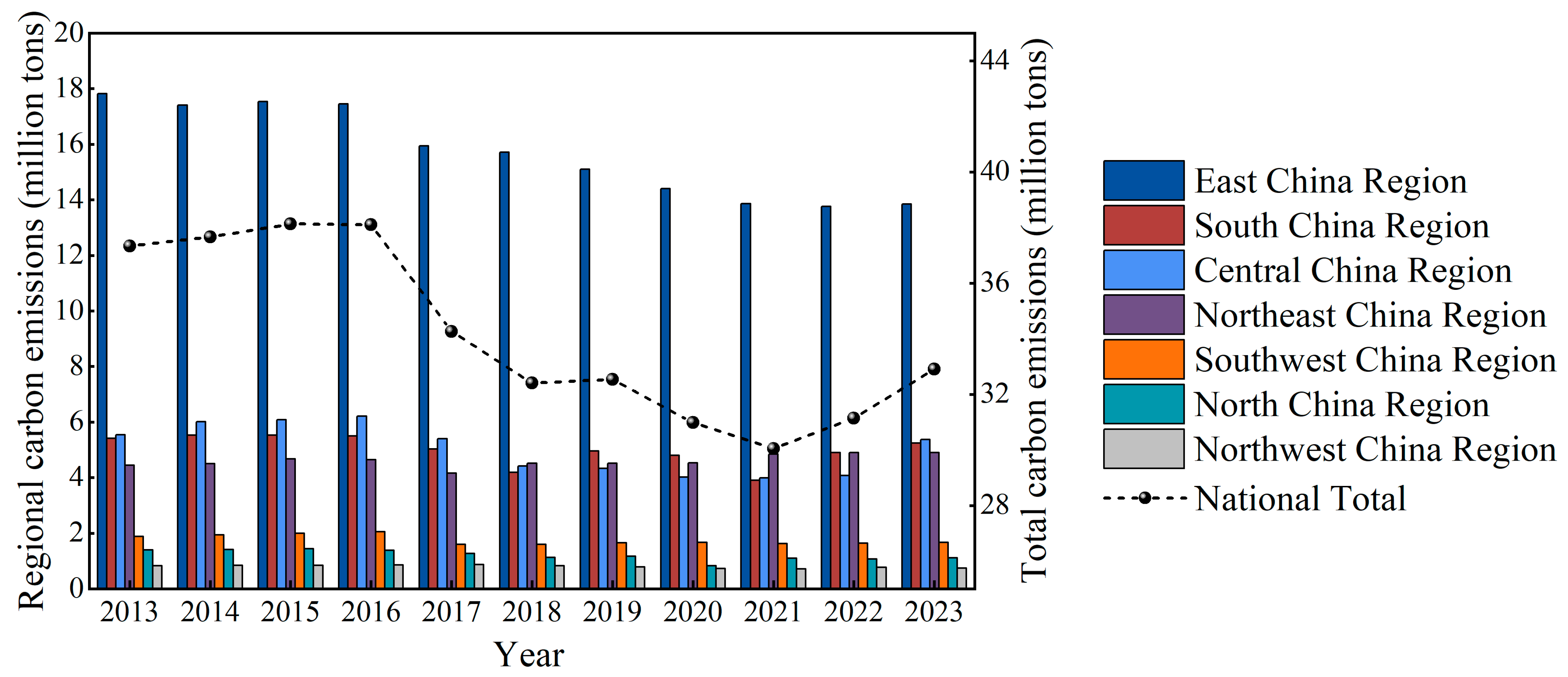
During the period from 2013 to 2023, the total carbon emissions from China’s freshwater aquaculture industry exhibited a declining trend, decreasing from 37 million tons in 2013 to 33 million tons in 2023. The changing trend of these emissions followed an “N”-shaped pattern, indicating an initial increase, followed by a decrease, and then another rise in the total emissions. In 2015, the carbon emissions from freshwater aquaculture nationwide reached a peak of 38 million tons.

(2)

The Eastern China region stands as the primary contributor to carbon emissions from the freshwater aquaculture industry, with an annual average emission of 16 million tons, accounting for 46% of the total emissions. The average annual proportions of carbon emissions from the freshwater aquaculture industry in Southern China, Central China, and Northeast China are 15%, 15%, and 13%, respectively, all falling within the range of 13–15%. The proportions of carbon emissions from the freshwater aquaculture industry in Southwest China, Northern China, and Northwest China are 5.2%, 3.6%, and 2.4%, respectively, indicating a relatively minor contribution to the overall emissions.

(3)

The global Moran’s I index for carbon emissions in China’s freshwater aquaculture industry exhibits a decreasing trend; moreover, with p-values ≤ 0.0010 and z-scores > 3.3 during the period from 2013 to 2023, a 99% confidence level of significant spatial correlation is demonstrated, indicating the presence of distinct and stable clustering effects. The predominant types of clustering are primarily high-high clustering and low-low clustering. The overall number of high-high clustering samples exhibits a declining trend. It has decreased from an initial count of seven to four, with these samples predominantly concentrated in Anhui Province, Jiangxi Province, and Fujian Province within the Eastern China region. The samples exhibiting low-low clustering are primarily concentrated in the Northwest China, Northern China, and Southwest China regions, with a relatively stable distribution pattern.

(4)

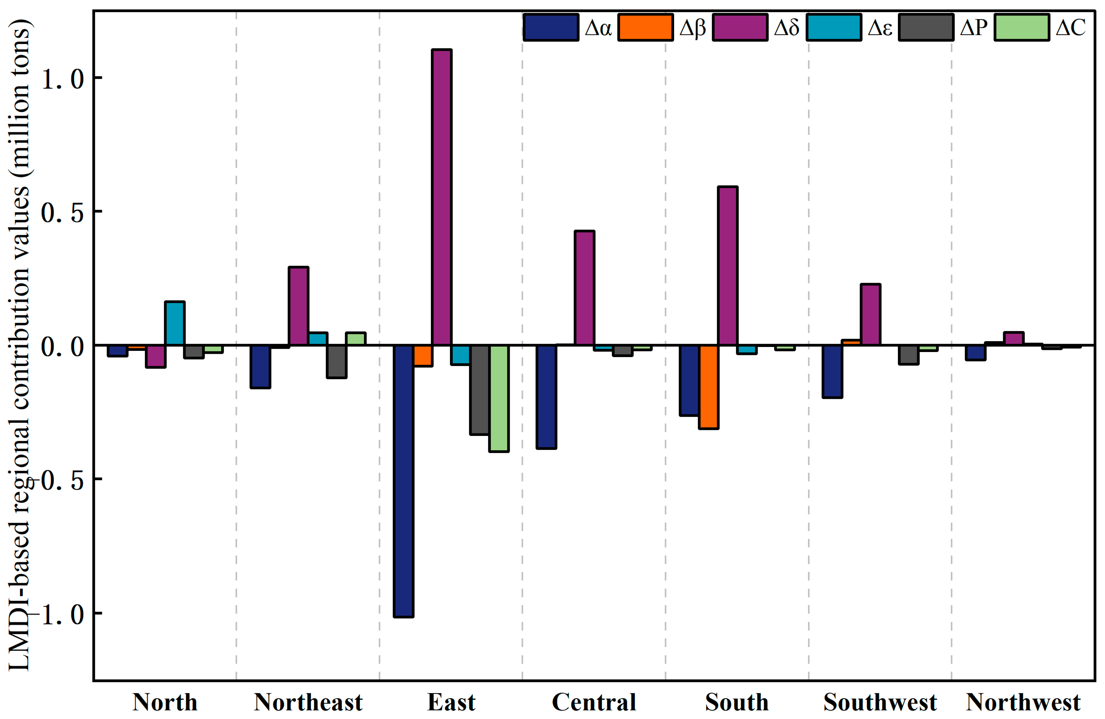
The LMDI decomposition model reveals that the level of economic development in the fisheries sector has exerted a positive and direct driving effect on the increase in carbon emissions. The production efficiency of freshwater aquaculture emissions, the industrial structure of freshwater aquaculture, and the scale of the aquaculture population in the fisheries sector all exhibit negative effects on carbon emissions in China’s freshwater aquaculture industry. The factor decomposition magnitudes are relatively significant in the Eastern China, Central China, and Southern China regions. The decomposition fluctuations are relatively small in Northern China, Northeast China, Southwest China, and Northwest China.

(5)

The decoupling elasticity between carbon emissions and economic growth in China’s freshwater aquaculture industry exhibits three states: weak decoupling, strong decoupling, and expansive negative decoupling. During the period from 2016 to 2021, alternating strong and weak decoupling effects were observed. This indicates that China’s freshwater aquaculture industry has been able to more effectively address carbon emission issues while driving economic growth, achieving coordinated development between the economy and the environment.

5.2. Recommendations

Based on the research findings presented above, this paper proposes the following three targeted recommendations:

(1)

According to China’s statistical data for 2020, 2022, and 2023, the freshwater product output in East China accounted for 42%, 43%, and 43% of the national total freshwater product output in those respective years. In response to the current situation where East China accounts for 46% of carbon emissions, a “one-province-one-policy” precision emission reduction mechanism should be established. For example, in high-high aggregation areas such as Anhui, Jiangxi, and Fujian Provinces, eco-friendly aquaculture models should be promoted, with policy subsidies guiding farmers to transform traditional practices and install tailwater treatment facilities. For regions like South China, Central China, and Northeast China (with proportions ranging from 13% to 15%), dynamic monitoring should be implemented, with carbon trading markets utilized to guide enterprises in optimizing their aquaculture models. For low-emission regions such as Southwest, North, and Northwest China (with proportions from 5.1% to 3.6%), a one-size-fits-all approach to emission reduction should be avoided; instead, green technology support should be provided to prevent the industrial decline caused by excessive pursuit of emission cuts.

(2)

Promote emission reduction technologies such as recirculating aquaculture systems and low-carbon equipment operation. Taking into account the negative driving effect of production efficiency in the Logarithmic Mean Divisia Index (LMDI) model, set targets for reducing the carbon emission intensity per unit of output. Gradually phase down high-carbon aquaculture models (e.g., extensive pond aquaculture) and expand the proportion of ecological aquaculture. Leverage the positive driving effect of the fisheries economic level to enhance product added value through green certification. Considering the economic impacts and the negative effect caused by the scale of the aquaculture population, it is essential to clarify the relationship between economic development and carbon emissions, aiming to achieve concurrent economic growth and a gradual reduction in carbon emissions. Meanwhile, conduct skills training for practitioners and promote the integration of small-scale aquaculture farmers into cooperatives or leading enterprises to minimize ineffective carbon emissions.

(3)

Sustain the state of strong decoupling (as demonstrated by the experience from 2016 to 2021) by providing financial subsidies and tax incentives to encourage freshwater aquaculture practitioners to adopt low-carbon technologies. Furthermore, integrate carbon emission intensity into the performance evaluation system for local governments to prevent carbon emissions from rebounding due to economic fluctuations.

References

1. Li, S.; Liu, L.; Suo, Y.; Li, X.; Zhou, J.; Jiang, Z.; Guan, H.; Sun, G.; Yu, L.; Liu, P.; et al. Carbon Tectonics: A new paradigm for Earth system science. Chin. Sci. Bull. 2023, 68, 309–338. [Google Scholar] [CrossRef]
2. Du, Y.; Liu, H.; Huang, H.; Li, X. The carbon emission reduction effect of agricultural policy—Evidence from China. J. Clean. Prod. 2023, 406, 137005. [Google Scholar] [CrossRef]
3. Yuan, J.; Xiang, J.; Liu, D.; Kang, H.; He, T.; Kim, S.; Lin, Y.; Freeman, C.; Ding, W. Rapid growth in greenhouse gas emissions from the adoption of industrial-scale aquaculture. Nat. Clim. Change 2019, 9, 318–322. [Google Scholar] [CrossRef]
4. MacLeod, M.J.; Hasan, M.R.; Robb, D.H.F.; Mamun-Ur-Rashid, M. Quantifying greenhouse gas emissions from global aquaculture. Sci. Rep. 2020, 10, 11679. [Google Scholar] [CrossRef] [PubMed]
5. Froehlich, H.E.; Runge, C.A.; Gentry, R.R.; Gaines, S.D.; Halpern, B.S. Comparative terrestrial feed and land use of an aquaculture-dominant world. Proc. Natl. Acad. Sci. USA 2018, 115, 5295–5300. [Google Scholar] [CrossRef]
6. Zhang, W.; Belton, B.; Edwards, P.; Henriksson, P.J.G.; Little, D.C.; Newton, R.; Troell, M. Aquaculture will continue to depend more on land than sea. Nature 2022, 603, E2–E4. [Google Scholar] [CrossRef]
7. FAO. The State of World Fisheries and Aquaculture; FAO: Rome, Italy, 2007; Volume 4, pp. 40–41. [Google Scholar]
8. Rosentreter, J.A.; Borges, A.V.; Deemer, B.R.; Hogerson, M.A.; Eyre, B.D. Half of global methane emissions come from highly variable aquatic ecosystem sources. Nat. Geosci. 2021, 14, 225–230. [Google Scholar] [CrossRef]
9. Saunois, M.; Stavert, A.R.; Poulter, B.; Bousquet, P.; Zhuang, Q. The Global Methane Budget 2000–2017. Earth Syst. Sci. Data Discuss. 2020, 12, 1561–1623. [Google Scholar] [CrossRef]
10. Zhang, L.; Wang, X.; Huang, L.; Wang, C.; Gao, Y.; Peng, S.; Canadell, J.G.; Piao, S. Inventory of methane and nitrous oxide emissions from freshwater aquaculture in China. Commun. Earth Environ. 2024, 5, 531. [Google Scholar] [CrossRef]
11. Gephart, J.A.; Henriksson, P.J.G.; Parker, R.W.R.; Shepon, A.; Gorospe, K.D.; Bergman, K.; Eshel, G.; Golden, C.D.; Halpern, B.S.; Hornborg, S.; et al. Environmental performance of blue foods. Nature 2021, 597, 360–365. [Google Scholar] [CrossRef] [PubMed]
12. Doney, S.C.; Ruckelshaus, M.; Duffy, J.E.; Barry, J.P.; Chan, F.; English, C.A.; Galindo, H.M.; Grebmeier, J.M.; Hollowed, A.B.; Knowlton, N.; et al. Climate Change Impacts on Marine Ecosystems. Annu. Rev. Mar. Sci. 2012, 4, 11–37. [Google Scholar] [CrossRef] [PubMed]
13. Solomon, S.; Qin, D.; Manning, M.; Chen, Z.; Marquis, M.; Averyt, K.B.; Tignor, M.; Miller, H.L. IPCC Fourth Assessment Report (AR4). In The Physical Science Basis: Contribution of Working Group I to the Fourth Assessment Report of the Intergovernmental Panel on Climate Change; Cambridge University Press: Cambridge, UK; New York, NY, USA, 2007; Volume 18, pp. 95–123. Available online: http://www.ipcc.ch (accessed on 20 June 2025).
14. IPCC. Climate Change 2022: Impacts, Adaptation and Vulnerability [EB/OL]. Available online: https://www.ipcc.ch/report/sixth-assessment-report-working-group-ii/ (accessed on 20 June 2025).
15. Natchimuthu, S.; Selvam, B.P.; Bastviken, D. Influence of weather variables on methane and carbon dioxide flux from a shallow pond. Biogeochemistry 2014, 119, 403–413. [Google Scholar] [CrossRef]
16. Bastviken, D.; Cole, J.J.; Pace, M.L.; Tranvik, L.J. Methane emissions from lakes: Dependence of lake characteristics, two regional assessments, and a global estimate. Glob. Biogeochem. Cycles 2004, 18, 12. [Google Scholar] [CrossRef]
17. Shao, G.; Kong, H.; Yu, J.; Li, C. Research on the Decomposition of Driving Factors of Carbon Emissions in China’s Marine Fishery Based on the LMDI Method. J. Agrotech. Econ. 2015, 6, 119–128. [Google Scholar]
18. Zhang, Y.; Bleeker, A.; Liu, J. Nutrient discharge from China’s aquaculture industry and associated environmental impacts. Environ. Res. Lett. 2015, 10, 045002. [Google Scholar] [CrossRef]
19. Xiao, X.; Agusti, S.; Lin, F.; Li, K.; Pan, Y.; Yu, Y.; Zheng, Y.; Wu, J.; Duarte, C.M. Nutrient removal from Chinese coastal waters by large-scale seaweed aquaculture. Sci. Rep. 2017, 7, 46613. [Google Scholar] [CrossRef] [PubMed]
20. Yang, P.; He, Q.; Huang, J.; Tong, C. Fluxes of greenhouse gases at two different aquaculture ponds in the coastal zone of southeastern China. Atmos. Environ. 2015, 115, 269–277. [Google Scholar] [CrossRef]
21. Huttunen, J.T.; Alm, J.; Liikanen, A.; Juutinen, S.; Larmola, T.; Hammar, T.; Silvola, J.; Martikainen, P.J. Fluxes of methane, carbon dioxide and nitrous oxide in boreal lakes and potential anthropogenic effects on the aquatic greenhouse gas emissions. Chemosphere 2003, 52, 609–621. [Google Scholar] [CrossRef]
22. Jingying, W. Carbon Emission Efficiency of Freshwater Aquaculture in China; Huazhong Agricultural University: Wuhan, China, 2021. [Google Scholar]
23. Long, R.; Shao, T.; Chen, H. Spatial econometric analysis of China’s province-level industrial carbon productivity and its influencing factors. Appl. Energy 2016, 166, 210–219. [Google Scholar] [CrossRef]
24. Ma, Y.; Sun, L.; Liu, C.; Yang, X.; Zhou, W.; Yang, B.; Schwenke, G.; Liu, D.L. A comparison of methane and nitrous oxide emissions from inland mixed-fish and crab aquaculture ponds. Sci. Total Environ. 2018, 637–638, 517–523. [Google Scholar] [CrossRef]
25. Martins, C.I.M.; Eding, E.H.; Verdegem, M.C.J.; Heinsbroek, L.T.N.; Schneider, O.; Blancheton, J.P.; d’Orbcastel, E.R.; Verreth, J.A.J. New developments in recirculating aquaculture systems in Europe: A perspective on environmental sustainability. Aquac. Eng. 2010, 43, 83–93. [Google Scholar] [CrossRef]
26. Cao, L.; Naylor, R.; Henriksson, P.; Leadbitter, D.; Metian, M.; Troell, M.; Zhang, W. China’s aquaculture and the world’s wild fisheries. Science 2015, 347, 133–135. [Google Scholar] [CrossRef]
27. Pauly, D.; Zeller, D. Comments on FAOs State of World Fisheries and Aquaculture (SOFIA 2016). Mar. Policy 2017, 77, 176–181. [Google Scholar] [CrossRef]
28. Xiao, Q.; Hu, C.; Gu, X.; Zeng, Q.; Liu, Z.; Xiao, W.; Zhang, M.; Hu, Z.; Wang, W.; Luo, J.; et al. Aquaculture farm largely increase indirect nitrous oxide emission factors of lake. Agric. Ecosyst. Environ. 2023, 341, 108212. [Google Scholar] [CrossRef]
29. Chen, Y.; Dong, S.; Wang, F.; Gao, Q.; Tian, X. Carbon dioxide and methane fluxes from feeding and no-feeding mariculture ponds. Environ. Pollut. 2020, 212, 489–497. [Google Scholar] [CrossRef] [PubMed]
30. China Fishery Statistical Yearbook (2014–2023). China Agriculture Press, Beijing, China. Available online: https://www.stats.gov.cn/ (accessed on 20 June 2025).
31. China Statistical Yearbook. Available online: https://www.stats.gov.cn/ (accessed on 20 June 2025).
32. National Bureau of Statistics. Available online: https://data.stats.gov.cn/index.htm (accessed on 20 June 2025).
33. Daqing, W.; Lichen, L. Decoupling relationship and driving factors between carbon emissions and economic growth in China’s freshwater aquaculture industry: Based on Tapio decoupling and LMDI model. J. Fish. China 2024, 49, 059618. [Google Scholar]
34. Field, C.B.; Barros, V.R.; Change, I.P.C. Contribution of Working Group II to the Fifth Assessment Report of the Intergovernmental Panel on Climate Change. In IPCC, 2014: Climate Change 2014: Impacts, Adaptation, and Vulnerability. Part A: Global and Sectoral Aspects; Guangdong Agricultural Sciences: Guangzhou, China, 2014. [Google Scholar]
35. Hao, X.; Huang, L.; Jianhua, Z.; Qi, M.; Jian, S.; Li, J. Calculation of energy consumption in China’s fishery industry. China Fish. 2007, 11, 74–76. [Google Scholar]
36. Weixue, L.; Benfeng, W. Reasonable allocation and proper use of aquaculture machinery. Fujian Agric. 2013, 7, 33. [Google Scholar]
37. Quan, G.; Gang, L.; Guohong, H. Some experiences using the feeder machine. Fish. Mod. 2002, 3, 30. [Google Scholar]
38. Xuehui, Y.; Yuqing, S.; Qifeng, H.; Sheng, L.; Jiaoli, J.; Caili, L. Comparative test on power consumption differences of aerators with different structural types. Mod. Agric. Equip. 2017, 4, 20–22. [Google Scholar]
39. Dong, Y.D.; Min, W.L.; Qian, W.; Si, Z.Y. GHG Emissions Estimation and Efficiency Analysis of Marine Fisheries. J. Shanxi Agric. Sci. 2013, 41, 873–876. [Google Scholar]
40. Huang, L.; Xuan, C. Elementary study on evaluation of CO2 emissions from aquaculture in China. South China Fish. Sci. 2010, 6, 77–80. [Google Scholar]
41. Jia, L.; Wang, M.; Yang, S.; Zhang, F.; Wang, Y.; Li, P.; Ma, W.; Sui, S.; Liu, T.; Wang, M. Analysis of Agricultural Carbon Emissions and Carbon Sinks in the Yellow River Basin Based on LMDI and Tapio Decoupling Models. Sustainability 2024, 16, 468. [Google Scholar] [CrossRef]
42. Zhang, C.; Lv, W.; Zhang, P.; Song, J. Multidimensional spatial autocorrelation analysis and it’s application based on improved Moran’s I. Earth Sci. Inform. 2023, 16, 3355–3368. [Google Scholar] [CrossRef]
43. Isik, M.; Sarica, K.; Ari, I. Driving forces of Turkey’s transportation sector CO2 emissions: An LMDI approach. Transp. Policy 2020, 97, 210–219. [Google Scholar] [CrossRef]
44. Jain, S.; Rankavat, S. Analysing driving factors of India’s transportation sector CO2 emissions: Based on LMDI decomposition method. Heliyon 2023, 9, 16. [Google Scholar] [CrossRef]
45. Ang, B.W. The LMDI approach to decomposition analysis: A practical guide. Energy Policy 2005, 33, 867–871. [Google Scholar] [CrossRef]
46. Karakaya, E.; Bostan, A.; Za, M. Decomposition and decoupling analysis of energy-related carbon emissions in Turkey. Environ. Sci. Pollut. Res. 2019, 26, 32080–32091. [Google Scholar] [CrossRef]
47. Tapio, P. Towards a theory of decoupling: Degrees of decoupling in the EU and the case of road traffic in Finland between 1970 and 2001. Transp. Policy 2005, 12, 137–151. [Google Scholar] [CrossRef]
48. Bin, L.; Jun, Z.X. Potential for Carbon Sink Fishery Development in Guizhou Province. J. Hydroecol. 2023, 44, 79–85. [Google Scholar]
49. Jingye, L.; Jue, L. Research on the Decoupling Effect, Driving Factors and Forecast of China’s Carbon Emissions. Environ. Sci. Technol. 2022, 45, 210–220. [Google Scholar]
50. Qing, H.; Junbiao, Z. Research on the Dynamic Evolution and Driving Factors of Agricultural Carbon Emissions in Major Grain-Producing Areas. Ecol. Econ. 2023, 39, 123–128. [Google Scholar]
Figure 1. Trend of carbon emissions from freshwater aquaculture in China from 2013 to 2023.
Water 17 02282 g001
Figure 2. Distribution map of local Moran’s I for carbon emissions from freshwater aquaculture in China for the years 2013, 2015, 2017, 2019, 2021, and 2023.
Water 17 02282 g002
Figure 3. Decomposition contribution degree of China’s freshwater aquaculture carbon emissions using the LMDI model from 2013 to 2023. Δα is the production efficiency of freshwater aquaculture emissions, Δβ is the industrial structure of the freshwater aquaculture industry, Δδ is the level of fishery economic development, Δε is the level of fishery farming development, and ΔP is the number of people engaged in fishery farming.
Water 17 02282 g003
Figure 4. Decomposition contribution degree of carbon emissions from freshwater aquaculture in different regions of China from 2013 to 2023 based on the LMDI model.
Water 17 02282 g004