Evaluation of Wake Structure Induced by Helical Hydrokinetic Turbine

Abstract

This study investigates the downstream wake characteristics of a helical hydrokinetic turbine through combined experimental and numerical analyses. A four-bladed helical turbine with a 20 cm rotor diameter and blockage ratio of 53.57% was tested in an open water channel under a flow rate of 180 m³/h, corresponding to a Reynolds number of approximately 90 × 10³. Velocity measurements were collected at 13 downstream cross-sections using an Acoustic Doppler Velocimeter, with each point sampled repeatedly. Standard error analysis was applied to quantify measurement uncertainty. Complementary numerical simulations were conducted in ANSYS Fluent using a steady-state k-ω Shear Stress Transport (SST) turbulence model, with a mesh of 4.7 million elements and mesh independence confirmed. Velocity deficit and turbulence intensity were employed as primary parameters to characterize the wake structure, while the analysis also focused on the recovery of cross-sectional velocity profiles to validate the extent of wake influence. Experimental results revealed a maximum velocity deficit of over 40% in the near-wake region, which gradually decreased with downstream distance, while turbulence intensity exceeded 50% near the rotor and dropped below 10% beyond 4 m. In comparison, numerical findings showed a similar trend but with lower peak velocity deficits of 16.6%. The root mean square error (RMSE) and mean absolute error (MAE) between experimental and numerical mean velocity profiles were calculated as 0.04486 and 0.03241, respectively, demonstrating reasonable agreement between the datasets. Extended simulations up to 30 m indicated that flow profiles began to resemble ambient conditions around 18–20 m. The findings highlight the importance of accurately identifying the downstream distance at which the wake effect fully dissipates, as this is crucial for determining appropriate inter-turbine spacing. The study also discusses potential sources of discrepancies between experimental and numerical results, as well as the limitations of the modeling approach.

1. Introduction

In recent years, the increasing demand for renewable and sustainable energy sources has driven significant research and technological development in the field of clean energy [1,2]. Among various alternatives, hydropower remains a prominent option due to its ability to provide consistent energy output with minimal environmental impact.

River turbines, a type of hydrokinetic turbine, harness the kinetic energy of flowing water to generate electricity, offering a hydrokinetic solution that operates without the need for dams [3,4,5]. These turbines are typically installed on the riverbed or suspended in the water column, allowing continuous energy production from natural water currents. River turbines eliminate the need for large-scale and invasive infrastructure typically associated with conventional hydropower plants. They offer several advantages such as modular design, ease of deployment, minimal site preparation, simple maintenance procedures, and the capability for easy retrieval or relocation based on operational or environmental requirements [6].

Helical hydrokinetic turbines, most notably the Gorlov Helical Turbine (GHT), harness the kinetic energy of flowing water through their continuously twisted blades [7]. This helical geometry, evolving from the straight-bladed Darrieus design, ensures that at any rotor position the blades maintain a favorable angle of attack, resulting in smoother torque profiles, reduced vibration, and improved self-starting [3,8,9].

In hydrokinetic energy systems, the wake effect refers to the flow disturbance that forms downstream of a turbine due to the extraction of kinetic energy from the water current [10]. To characterize the wake effect, velocity deficit and turbulence intensity are commonly used as primary indicators [11,12]. The velocity deficit refers to the reduction in streamwise velocity within the wake region compared to the undisturbed upstream flow, reflecting the loss of kinetic energy. Turbulence intensity, on the other hand, quantifies the level of velocity fluctuations relative to the mean flow and indicates the degree of unsteadiness and mixing induced by the turbine [13].

As water flows through the turbine rotor, it experiences a reduction in velocity and an increase in turbulence, resulting in a wake characterized by velocity deficit and turbulent mixing, as well as sometimes in rotational (swirl) motion. This disturbed region extends for several rotor diameters (RDs) downstream and significantly affects the performance of any subsequent turbines placed in that zone [14].

The severity and spatial extent of the wake are influenced by several factors, including the turbine’s tip speed ratio, blade geometry, velocity deficit ambient turbulence intensity, and the degree of channel confinement [15]. In particular, higher blockage ratios and shallow flow conditions tend to intensify the wake effect and prolong wake recovery [16]. The near wake region, typically within 2 to 5 RD downstream, is dominated by coherent vortex structures and strong shear gradients, while the far wake gradually returns to ambient flow conditions through momentum diffusion and turbulent mixing [17]. The process by which the flow recovers from the velocity deficit and turbulent fluctuations is referred to as wake recovery [18]. This wake recovery distance plays a critical role in multi-turbine installations, as insufficient spacing between turbines may result in significant power losses and increased structural fatigue in downstream units due to unsteady loading [19].

To analyze and predict the development and recovery of the wake, Computational Fluid Dynamics (CFD) is extensively employed using turbulence models [20,21]. Nevertheless, numerical results must be validated through physical measurements. Experimental studies conducted in open water channels using techniques such as Acoustic Doppler Velocimetry (ADV) and Particle Image Velocimetry (PIV) provide high-resolution velocity data, which are essential for capturing the three-dimensional wake structure and for benchmarking simulation results [22].

Riglin et al. (2016) [23] conducted a numerical investigation focused on the performance characteristics of hydrokinetic turbine arrays designed for riverine applications. The study utilized a horizontal-axis turbine with a rotor diameter of 0.5334 m. Steady-state, three-dimensional flow fields were resolved using the k-ω Shear Stress Transport (SST) turbulence model. The simulation results demonstrated that the wake dissipated laterally within approximately 2.5 RD and longitudinally by around 6 RD. Under identical operating conditions, the downstream turbines deployed in the array configuration achieved only 20% or less of the power output produced by a single, isolated turbine, highlighting the significant impact of upstream wake interactions.

In the numerical study conducted by Silva et al. [24], the wake generated by a horizontal-axis hydrokinetic turbine was simulated. The study employed a three-bladed axial-flow turbine with a diameter of 10 m, and the numerical results were validated against experimental data from the NREL Phase VI wind turbine. All simulations were carried out using the Unsteady Reynolds-Averaged Navier–Stokes (URANS) approach combined with the Shear Stress Transport (SST) turbulence model, implemented through ANSYS CFX software. The results revealed that the wake extended approximately 3 RD in the near wake and 12 RD in the far wake, with the axial velocity fully recovering at a downstream distance of 12 RD.

Chen et al. [22] performed an experimental study to evaluate the wake behavior downstream of a horizontal-axis tidal turbine. The experiments employed a three-bladed device with a rotor diameter of 0.3 m, installed in a recirculating water flume. Three-dimensional velocity data were collected at sixteen downstream cross-sections extending up to 20 RD, using an Acoustic Doppler Velocimeter. The results showed that the maximum turbulence intensity reached 23%; even at 20 RD, it had not completely returned to the background turbulence level, remaining at approximately 5%. At 1 RD, the velocity deficit peaked at 51.6%, but this value dropped significantly to 20% by 5.5 RD and further diminished to around 5% at 20 RD.

Musa et al. [25] carried out an experimental investigation focusing on wake behavior and sediment dynamics associated with hydrokinetic turbines. The study employed a three-bladed axial-flow turbine featuring a rotor diameter of 0.15 m. According to the findings, the streamwise velocity exhibited a recovery of approximately 72% to 76% of its upstream value at a downstream distance equivalent to 6 RD.

Santos et al. [26] conducted a study on hydrokinetic turbine wake behavior by applying the actuator disk model alongside three-dimensional simulations incorporating realistic velocity profiles, geometric characteristics, and curvature data derived from an Amazonian river. The analysis was performed on a three-bladed turbine with a rotor diameter of 4 m. The investigation utilized Blade Element Momentum (BEM) theory in combination with ANSYS Fluent to evaluate wake dynamics. The authors explored three distinct turbine configurations and reported that the wake dissipation length varied between 7 and 9 rotor RD, depending on the layout and flow conditions.

In the numerical study conducted by Reddy and Bhosale [27], a vertical-axis helical hydrokinetic turbine was employed to evaluate the influence of blade count on wake characteristics. Transient flow simulations were performed using ANSYS-CFX, employing the k-ε Renormalization Group (RNG) turbulence model to resolve unsteady flow characteristics. The analysis revealed that increasing the number of blades leads to a notable rise in both velocity deficit and turbulence intensity within the wake region. Additionally, the time-averaged axial velocity was found to recover to approximately 95% of the freestream value at a downstream distance, ranging between 19 and 25 RD for the configurations examined.

In their literature review, Nago et al. [28] emphasized the critical importance of investigating the correlation between turbine diameter and the wake dissipation length for optimal turbine array configuration. The study also highlighted the limited scope of existing research on wake characterization, noting that the current understanding of the phenomenon remains incomplete. Furthermore, it was evident that accurately estimating wake behavior is inherently complex, with numerous uncertainties associated with the modeling approaches used to represent it.

In numerical studies focusing on the wake effect of hydrokinetic turbines, widely used computational tools include ANSYS Fluent, ANSYS CFX, and OpenFOAM [29]. These simulations typically employ URANS-based approaches, with turbulence models such as k-ε, k-ω SST, and RNG being commonly applied [28]. Particular attention is paid to mesh quality, time step selection, and boundary condition definition to ensure numerical accuracy. In experimental investigations, key wake parameters such as velocity deficit, turbulence intensity, wake length, and momentum diffusion are often measured to characterize wake behavior.

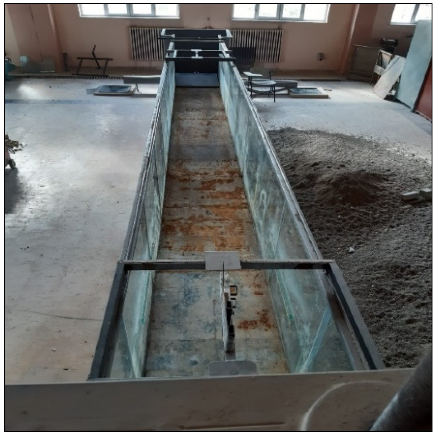
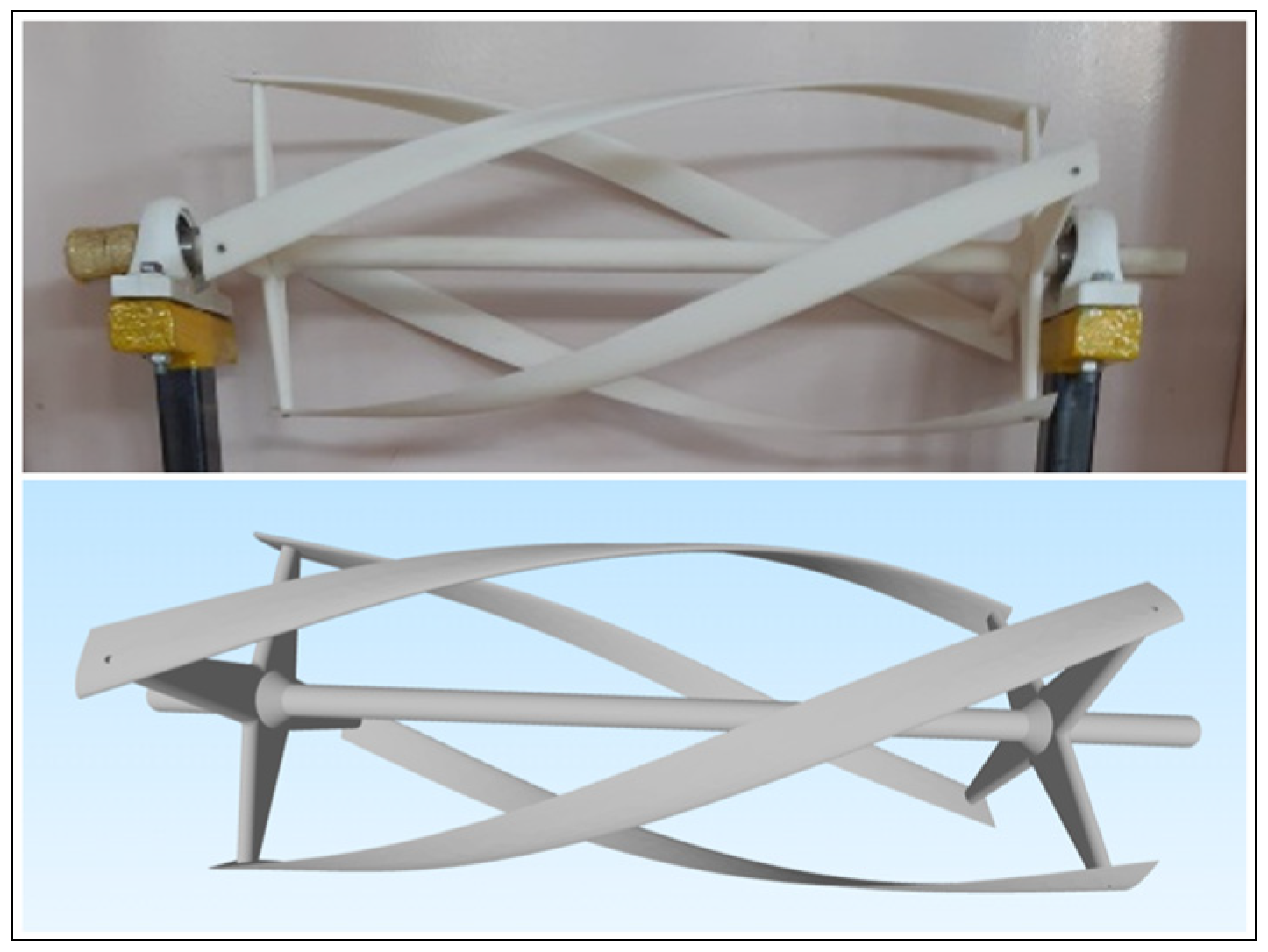
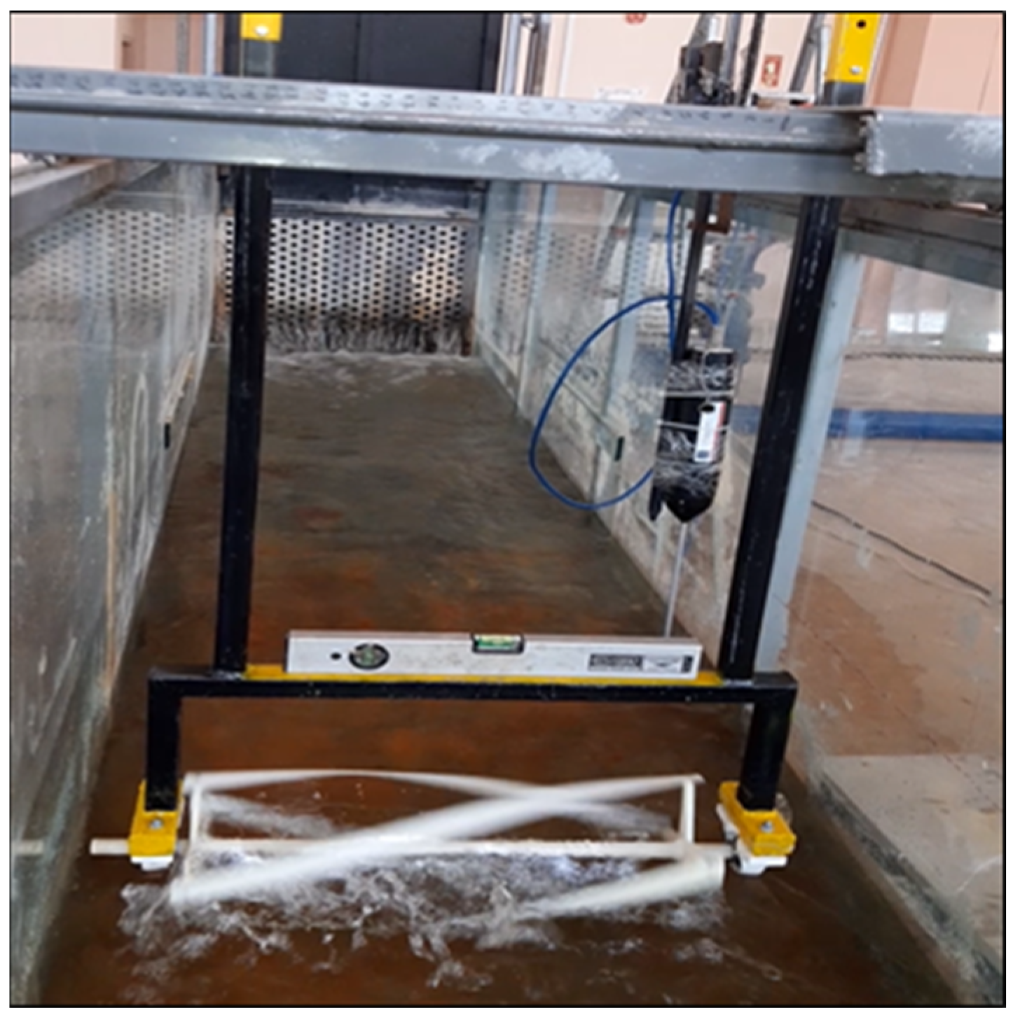
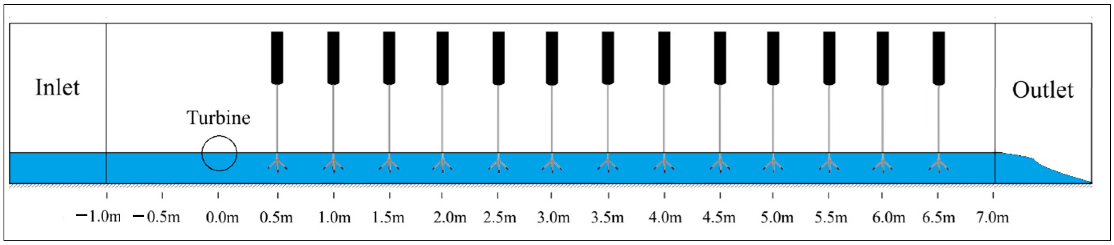
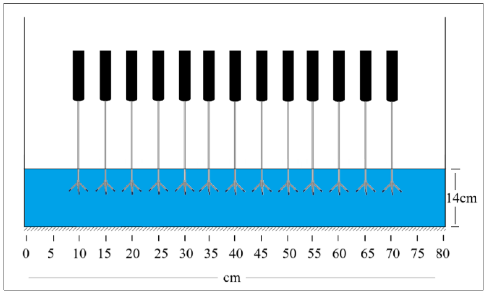
In this study, experimental analyses were performed in an open water channel using a small-scale, four-bladed, helical vertical axis turbine manufactured with a 3D printer. The channel used is a shallow channel with a length of 8 m and a width of 0.8 m. Numerical simulations were carried out by modeling the same turbine and channel geometry, ensuring consistency between the experimental and computational setups. Due to the 8 m length of the channel used in the experiments, experimental measurements were conducted up to this distance downstream of the turbine. In contrast, the numerical study extended the analysis up to 30 m. Velocity measurements up to 6.5 m downstream of the turbine were obtained both experimentally and numerically for comparison. Since the recovery trends of the velocity profiles were similar, further evaluations beyond this distance were based only on numerical results. In the literature, turbulence intensity and velocity deficit are commonly considered as key reference parameters in wake analysis, and turbine spacing is often based on these criteria returning to acceptable levels. Some studies [22] indicate that, even when these values are reached, cross-sectional velocity profiles may not fully recover, suggesting that residual wake effects may persist. Our understanding of the far wake region and precise wake recovery length remains limited. In the present study, alongside velocity deficit and turbulence intensity, recovery in cross-sectional velocity profiles downstream of the turbine was examined to achieve a more accurate determination of wake recovery length. The findings from this study are expected to provide useful insights into wake effects, wake recovery, and turbine array configuration for small-scale river turbine experiments conducted under open-channel laboratory conditions.

2. Materials and Equipment

2.1. Open Water Channel

The experimental study was conducted in an open water channel (Figure 1) operating in a recirculating manner using pumps. The channel is 8 m long and 0.8 m wide. A flow meter is installed on the inlet pipe supplying water to the channel. All experimental procedures were carried out under a constant flow rate of 180 m³/h corresponding to a Reynolds number of approximately 90 × 10³, while the downstream sluice gate remained fully open to minimize backwater effects. At the discharge of 180 m³/h, an average flow depth of approximately 14 cm was recorded along the channel.

2.2. Helical Hydrokinetic Turbine

In this study, a helical hydrokinetic turbine manufactured using a 3D printer with ABS (Acrylonitrile Butadiene Styrene) material was employed (Figure 2). The turbine had a width of 60 cm and a diameter of 20 cm. It consisted of four blades composed of optimized hydrofoil profiles, two star-shaped end disks, and a central shaft. Each blade was configured with a twist angle of 90 degrees. The shaft had a total length of 67 cm and was supported by two ball bearings, located at both ends. For the experimental setup, the shaft was positioned approximately 15 cm above the channel bottom, and the turbine was operated in a half-submerged condition, with the flow depth of approximately 14 cm allowing the turbine to be fully submerged up to the shaft level and to reach its maximum rotational speed. In this configuration, the blockage ratio, which represents the proportion of the channel cross-sectional area occupied by the turbine, was calculated as 53.57%. The turbine was securely mounted to a metallic support structure, which can move along rail-guided tracks fixed to the sidewalls of the channel, using a custom-designed metal bracket.

2.3. Velocimeter

A high-resolution a NORTEK Acoustic Doppler Velocimeter (ADV), (Nortek AS, Oslo, Norway) that is shown in Figure 3 was employed in the experimental study to capture the three-dimensional flow velocity field. The sampling frequency of the velocity measurement device was set to 200 Hz. Approximately 12,000 measurements were recorded at each point, and the mean values of these datasets were utilized for experimental analysis. The velocimeter was mounted on a secondary movable rail system installed above the channel, enabling velocity measurements to be conducted at specified lateral positions. All measurements were taken at a vertical distance of approximately 8.5 cm above the channel bed. The standard error ranges for the velocity measurements at each sampling point, calculated as mean velocity ± standard error, ranged from 0.054% to 0.491% of the mean velocity across all locations. Based on these standard error values, the 95% confidence intervals for the mean velocities at each point fall within a similarly low range, supporting the reliability of the measurements.

3. Methodology

3.1. Experimental Setup

Experimental research was carried out at a constant flow rate of 180 m³/h with an approximate water depth of 14 cm. Initially, the 3D-printed helical turbine was positioned at the 0.0 m mark, while the velocimeter was placed 0.5 m downstream. Subsequently, the turbine was kept fixed at the 0.0 m position, and the velocity measurement device was sequentially relocated to the following positions: 1.0 m, 1.5 m, 2.0 m, 2.5 m, 3.0 m, 3.5 m, 4.0 m, 4.5 m, 5.0 m, 5.5 m, 6.0 m, and 6.5 m (Figure 4). For each cross-section downstream of the turbine, 13 velocity measurements were conducted. The measurements were taken, starting 10 cm inward from both the left and right sidewalls of the channel (Figure 5). Each measurement was repeated multiple times (at least three times) to ensure accuracy and repeatability, allowing for the identification of any potential inconsistencies and the validation of the reliability of the experimental data. The narrow 0.8 m channel may increase flow interactions with the boundaries, potentially affecting lateral velocity profiles. However, while average velocities on the flow direction (x direction) were between 0.276 m/s and 0.516 m/s, y and z directions recorded values from 0.000 m/s to 0.015 m/s, indicating that sidewall effects are negligible in this study.

3.2. Numerical Modeling

In this study, the primary objective was to investigate time-averaged wake characteristics and provide general insights into wake recovery, for which the steady-state approach offers computational efficiency and reliable mean flow predictions when appropriate turbulence models are employed. Therefore, numerical simulations were performed using a steady-state solution approach.

The mesh structure in this study consisted of two separate domains: one defined around the turbine and the other representing the surrounding fluid region. For the turbine domain, approximately 1.5 million elements were generated, while the surrounding domain contained 3.2 million elements, resulting in a total mesh size of 4.7 million elements. The overall mesh exhibited an average element quality of 0.87 with a standard deviation of 0.095, and the average skewness value was 0.19 with a standard deviation of 0.028. The orthogonal quality averaged 0.81, with a standard deviation of 0.093. Mesh independence was assessed by starting with a mesh of 2 million elements and progressively refining the mesh up to 4.7 million elements, monitoring the mean velocity values. It was observed that the mean velocity values remained unchanged beyond 4.5 million elements, indicating mesh convergence. The interface between the turbine domain and the outer domain was defined as a matched boundary. Additionally, nine layers of inflation were applied around blade surfaces to better resolve the boundary layer.

The computational domain was constructed to represent the open water channel used in the experimental study, and the boundary conditions were defined accordingly. Channel walls were modeled with no-slip boundary conditions, while the rotational motion of the turbine blades was represented using the Multiple Reference Frame (MRF) method, which allows for the simulation of rotating components within a steady-state framework. Velocity inlet and pressure outlet boundary conditions were applied at the channel inlet and outlet, respectively. The k-ω SST turbulence model was employed. The turbulence conditions at the inlet and outlet boundaries were also set consistently. A coupled solver algorithm was used to ensure pressure–velocity coupling and to improve convergence. Second-order upwind schemes were applied for the discretization of the momentum and turbulence equations. The convergence criterion was set based on the root mean square (RMS) residuals, with a threshold of 10⁻⁵ for all governing equations. A mesh convergence study was conducted using multiple grid densities to verify mesh independence. In simulations, the channel width was set to 0.8 m, water depth to 0.14 m, and flow rate to 180 m³/h. The helical hydrokinetic turbine was positioned at the 0 m reference location, and flow velocities downstream of the turbine were obtained at the same measurement points as in the experimental setup.

4. Assessment of Turbine Output

4.1. Velocity Deficit

The velocity deficit is a key parameter used to quantify the reduction in flow velocity behind a hydrokinetic turbine due to energy extraction. It is calculated using the following non-dimensional Equation (1):

$$U_{def}=(1-{\displaystyle \frac{\overline{u_{tt}}}{\overline{u}}})\times 100\%$$

(1)

where U_def is the velocity deficit, $\overline{u_{tt}}$: is the mean velocity measured at a point downstream of the installed turbine, and $\overline{u}$ is the local time-averaged velocity measured at a specific downstream point behind the turbine.

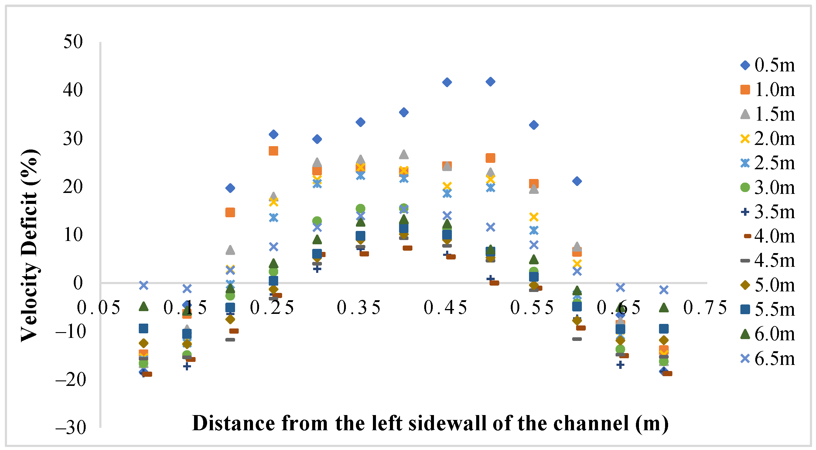
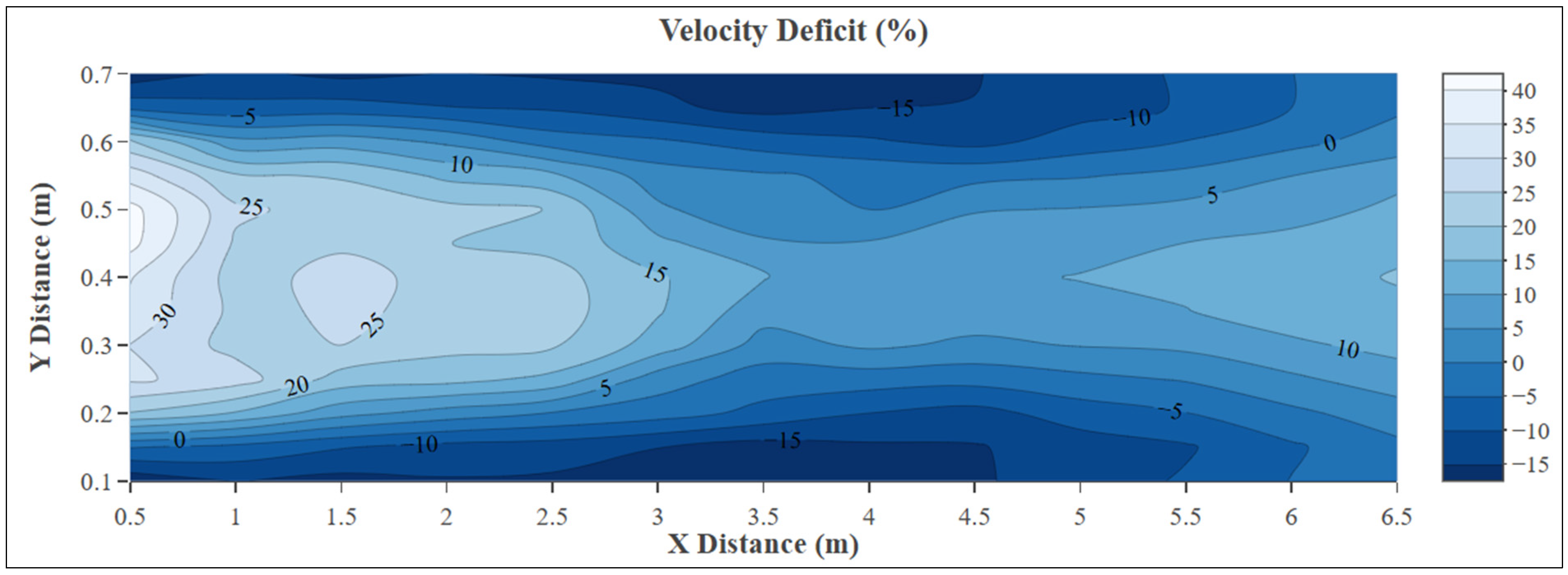
The experimental velocity deficit profiles (Figure 6) and counter map (Figure 7) of multiple downstream cross-sections (0.5 m to 6.5 m) demonstrates the clear evolution of the wake structure generated by the helical turbine. Maximum velocity deficit values were observed near the centerline of the channel (between 0.30 m and 0.50 m from the left sidewall), particularly at 0.5 m downstream, where the deficit exceeded 40%, indicating significant flow deceleration immediately behind the rotor. As the flow progresses downstream, a gradual reduction in deficit values is evident, reflecting the wake recovery process. Notably, while the magnitude of the velocity deficit decreases beyond 4.0 m, residual asymmetries and local fluctuations persist even at 6.5 m, suggesting that the wake has not fully dissipated. The slight increase in velocity deficit near the channel outlet may be attributed to the fully open boundary condition, which can induce reverse flow effects or disturb the recovery pattern in the far-wake region. The lateral velocity deficit profiles exhibit a characteristic double-hump shape near the mid-channel, with negative values near the sidewalls, consistent with wake expansion and flow redirection. These observations confirm the persistence of the wake effect over extended distances and highlight the importance of downstream flow characterization for assessing turbine performance and array placement in hydrokinetic systems.

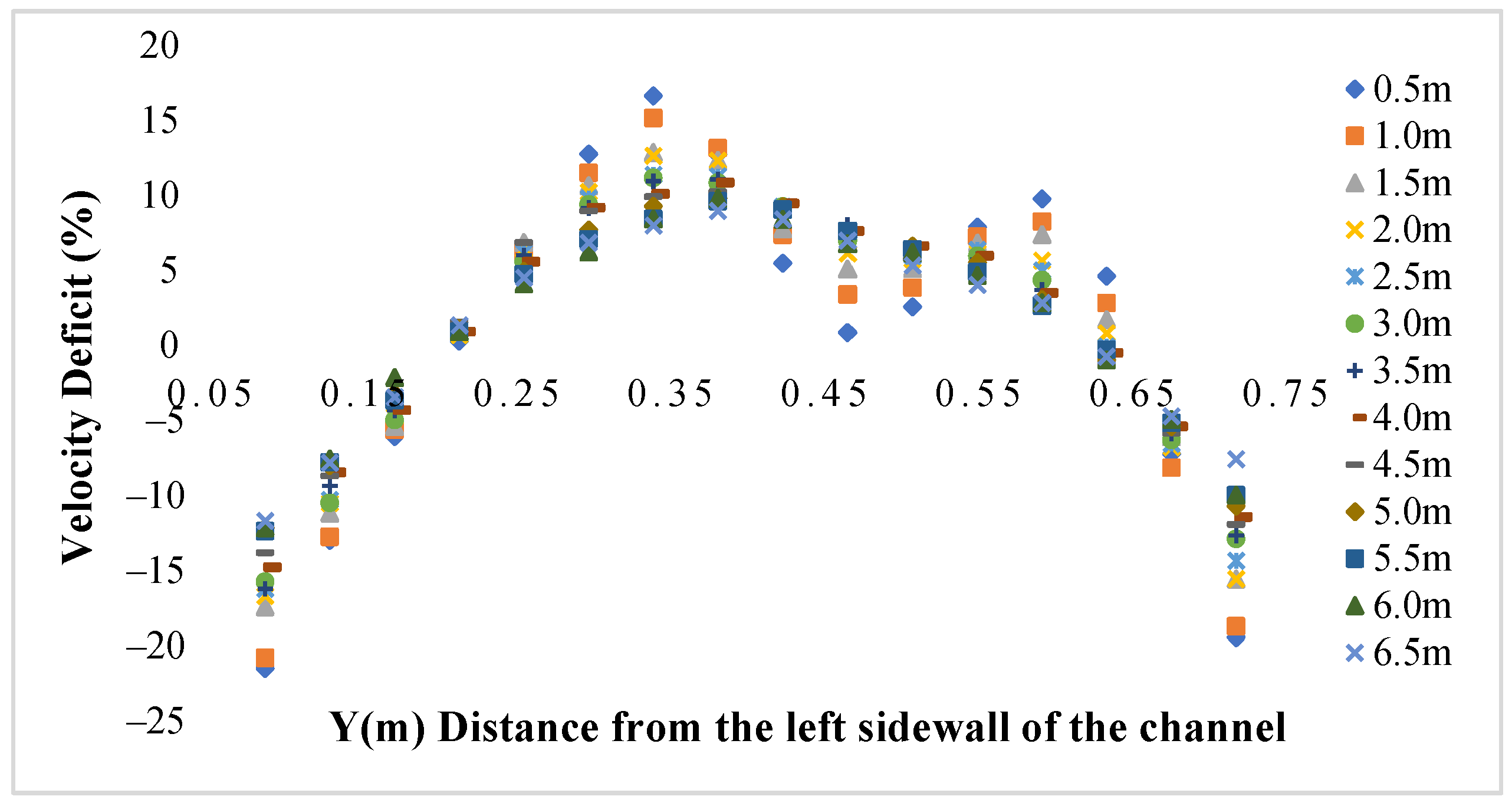
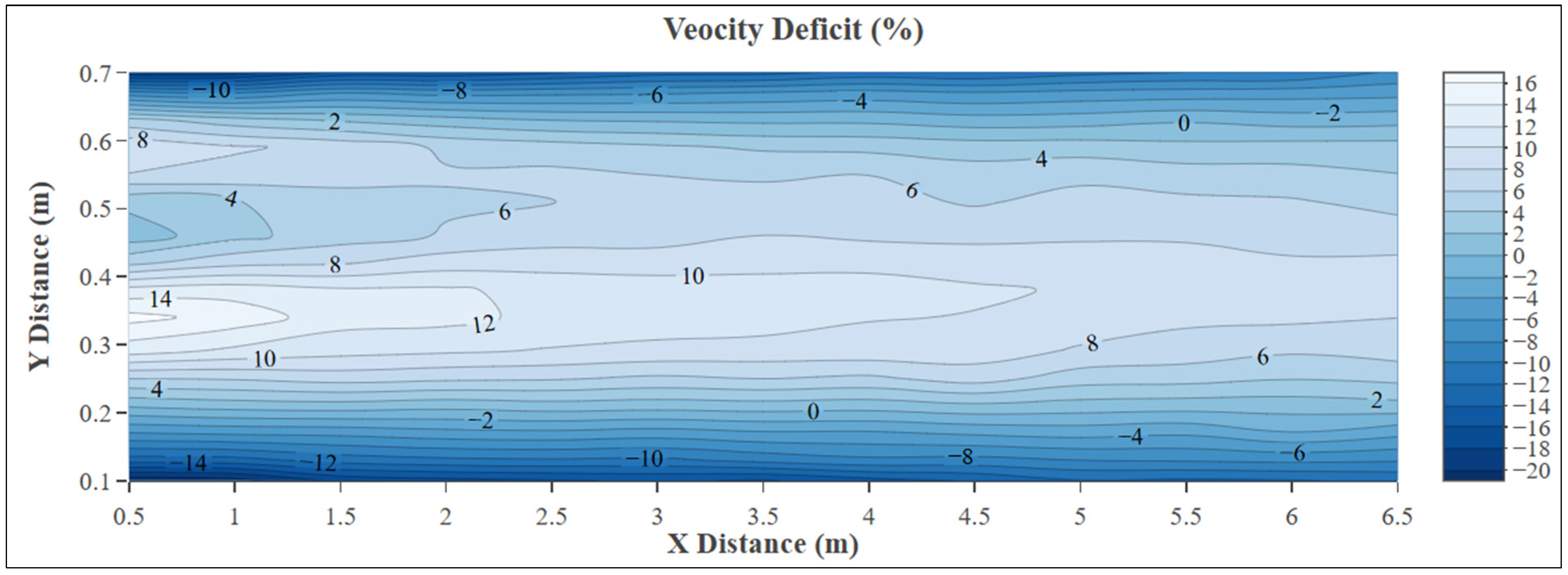
The numerical velocity deficit profiles (Figure 8) and counter map (Figure 9) show a well-defined wake structure formed behind the hydrokinetic turbine, extending up to 6.5 m downstream. Maximum velocity deficits are observed close to the channel center (between 0.30 m and 0.40 m from the left sidewall), especially at 0.5 m downstream, where values exceed 16%, peaking at 16.648%. This peak gradually diminishes along the streamwise direction, with the deficit values decreasing below 10% after approximately 4.5 m. Notably, the wake centerline remains consistently aligned and symmetric, and the lateral profiles maintain a characteristic bell-shaped structure. Velocity recovery is more pronounced between 3.0 m and 6.5 m, as the velocity deficit steadily decreases and approaches near-zero or slightly positive values, particularly in the mid-channel region, based on normalized velocity profiles. The presence of negative deficits near the sidewalls at all distances suggests persistent flow reversal or boundary effects. Overall, the numerical results depict a consistent and smooth wake decay pattern with clear axial symmetry.

A comparison between experimental and numerical velocity deficit profiles reveals both qualitative agreement and notable differences. Both datasets exhibit a symmetric wake pattern, with the highest deficits occurring in the central region of the channel and gradually diminishing downstream. In the experimental results, however, the peak velocity deficits are significantly higher (over 40% at 0.5 m) and the recovery is slower, with residual effects still present at 6.5 m. In contrast, the numerical simulation predicts lower peak deficits (maximum ~16.6%) and a smoother, more rapid recovery. The difference in peak velocity deficits may be attributed to the influence of real-world factors such as turbulence, flow irregularities, and boundary interactions present in the experimental setup, which are not captured under the controlled conditions of the numerical simulation, as well as the limitations of the turbulence model and the steady-state approach’s inability to fully resolve unsteady vortex dynamics. Both factors may contribute to the observed discrepancies between experimental and numerical results. As a result, the experimental results show higher and more persistent deficits, while the simulation yields lower peak values and smoother recovery. Additionally, the experimental data display slightly more lateral asymmetry and irregularities, likely due to real-world disturbances and probe interference. Despite these differences, the general trends and wake characteristics are consistent across both approaches, validating the numerical model as a reliable predictor of turbine-induced flow behavior, albeit with limitations in capturing fine-scale turbulence and local disturbances.

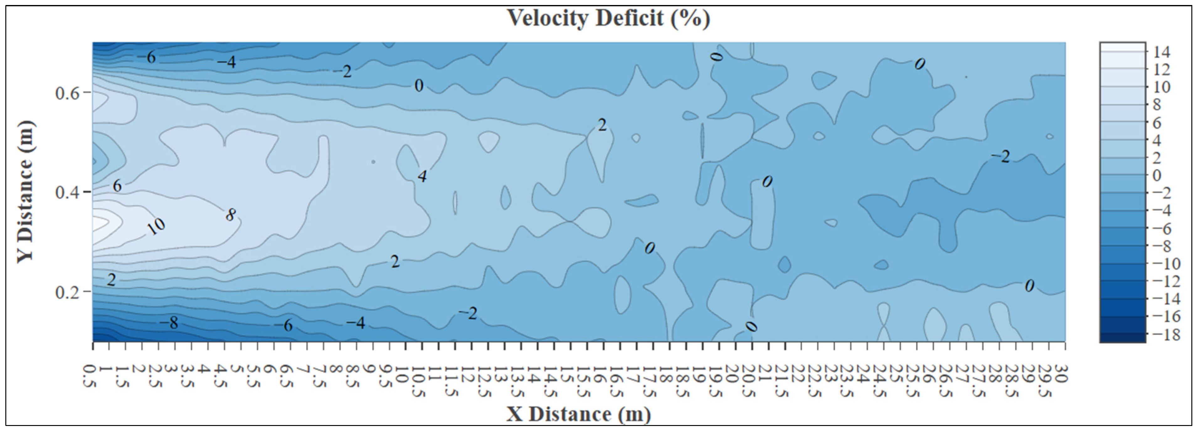
The numerical results for velocity deficit (Figure 10) along the centerline and lateral positions of the channel, extending from the turbine location 0.5 m to 30 m downstream, reveal a clear wake recovery trend. Maximum velocity deficits, ranging between −15% and −20%, are observed within the first 1–3 m after the turbine, particularly at mid-channel positions. Between 5 m and 10 m, a significant reduction in deficit magnitude occurs, with values decreasing to below −5% in most lateral sections, indicating the gradual re-acceleration and redistribution of the flow. Beyond 15 m, the velocity deficit becomes negligible or even transitions to slightly positive values across most of the cross-section, suggesting that the wake has nearly dissipated and the flow has returned to a more uniform, steady profile.

In the context of a tandem turbine array, where minimizing upstream wake interference is crucial for the downstream unit’s performance, the data suggests that the second turbine should ideally be placed no closer than 15 m downstream from the first turbine. At this location, the wake effects sufficiently subside, and the velocity field is more uniform, reducing the risk of reduced efficiency or increased fatigue loading due to turbulence. Therefore, the analysis shows that optimal spacing for a downstream turbine in serial configuration lies in the range of 15–20 m, ensuring minimal wake-induced performance degradation.

4.2. Turbulence Intensity

Turbulence intensity (TI) is a dimensionless measure of the fluctuation of velocity relative to the mean flow velocity in a fluid. It quantifies the strength of turbulence and is commonly expressed as a percentage. In wake effect analysis, turbulence intensity is used to evaluate how rapidly the wake recovers and how much it may disturb downstream turbines in an array. It is calculated with Equations (2) and (3) as follows:

$$\sigma =\sqrt{({\displaystyle \frac{1}{N}}{\sum }_1^N{(u_i-{\overline{u}}_i)}^2}$$

(2)

$$TI={\displaystyle \frac{\sigma }{{\overline{u}}_i}}\times 100\%$$

(3)

where σ is standard deviation of the velocity data, $u_i$ is the $i^{th}$ velocity measurement, ${\overline{u}}_i$ is mean velocity (time-averaged velocity at the measurement point), and N is the total number of velocity measurements.

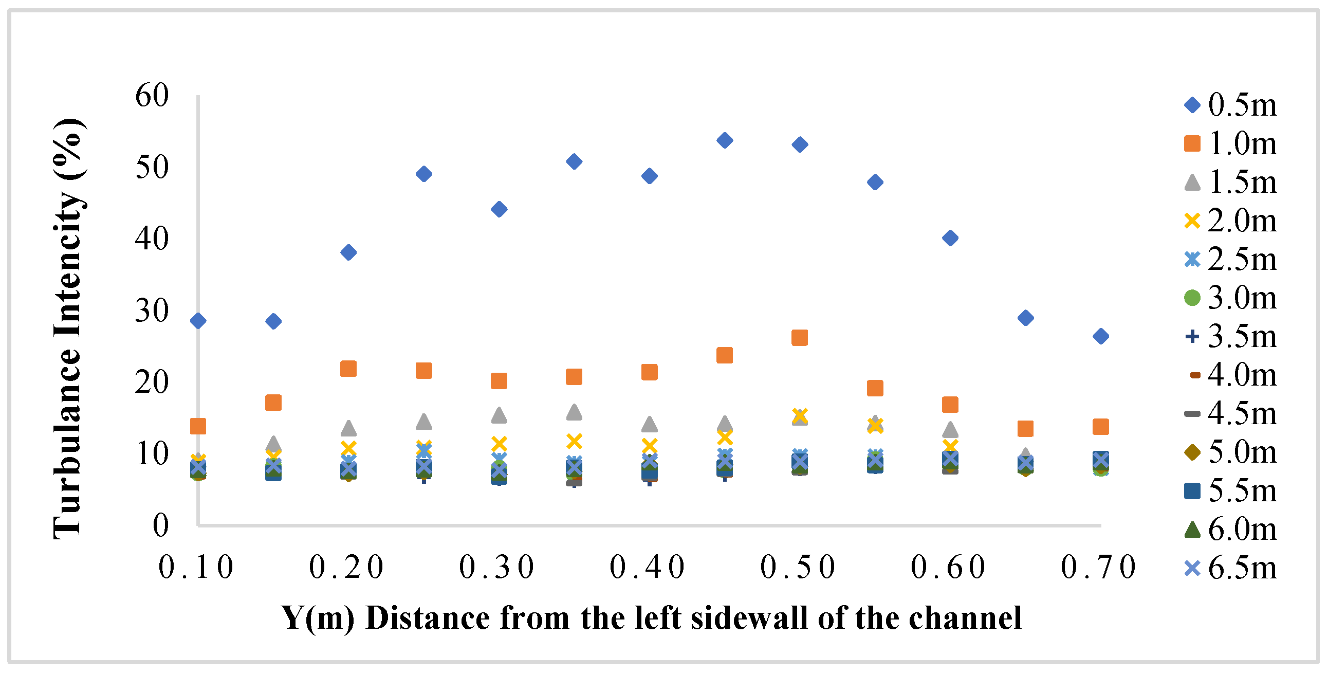
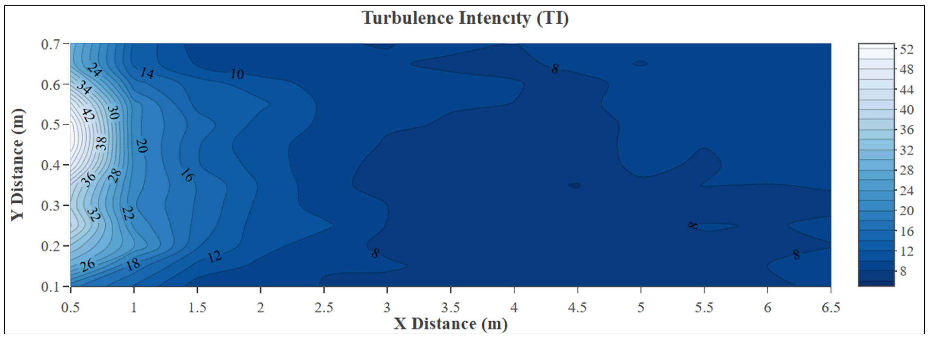
The turbulence intensity (TI) distribution (Figure 11) and counter map (Figure 12) of 13 lateral positions and 13 downstream sections from 0.5 m to 6.5 m provides insight into the wake-induced unsteadiness in the flow field downstream of the hydrokinetic turbine. As expected, TI values are significantly elevated in the near-wake region, with maximum values exceeding 50% at the mid-span of the channel (e.g., 0.45 m and 0.50 m lateral positions at 0.5 m downstream). These elevated turbulence levels are indicative of strong rotor-induced shear and vortex shedding. As the flow progresses downstream, the clear attenuation of TI is observed across the entire span of the channel. Between 1.0 m and 3.0 m, TI values decrease sharply, particularly in the central region, where values drop from over 20% to below 10%. This trend confirms the progressive dissipation of turbulence and energy redistribution as the wake recovers.

From 4.0 m onward, turbulence intensity stabilizes and fluctuates within a narrower range (~7–9%), indicating a transition toward a more developed and uniform flow. However, slight increases in TI are still noticeable beyond 5.0 m, particularly at off-center positions (e.g., 0.60 m and 0.70 m), likely due to lateral mixing and shear-layer interactions between wake and bypass flow. The overall pattern suggests that while the near-wake region is dominated by high turbulence and flow instability, the flow gradually stabilizes beyond 4–5 m, though residual unsteadiness persists across the channel width up to 6.5 m. Based on the statistical analysis, the standard errors for turbulence intensity ranged from 0.0011 to 0.0287. The 95% confidence intervals for the mean turbulence intensity values at each point were also narrow, providing additional evidence for the accuracy and repeatability of the experimental results.

4.3. Cross-Sectional Velocity Comparison

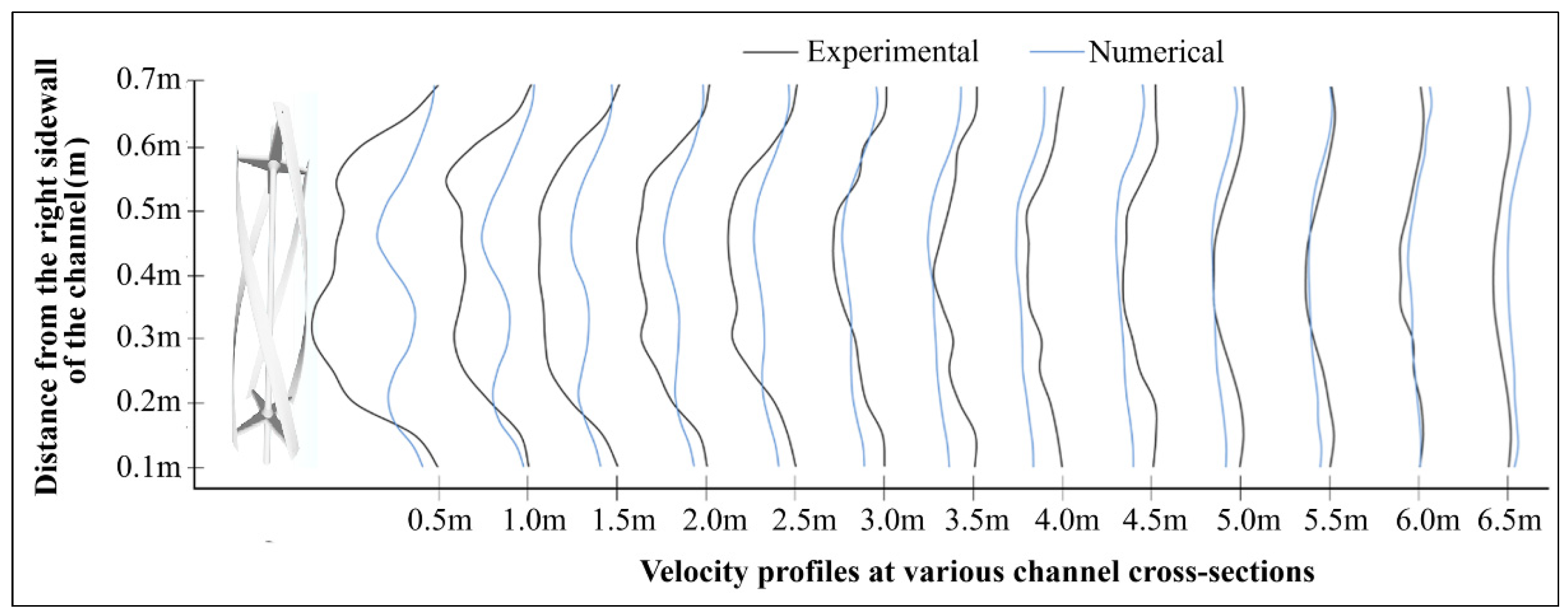
Velocity profiles obtained from experimental and numerical studies at various downstream positions from the hydrokinetic turbine are compared in Figure 13. In the near-wake region (0.5–2.5 m), the experimental profiles show more pronounced asymmetry and local peaks, while the numerical results exhibit smoother and more symmetric curves. From approximately 3.5 m onward, both profiles begin to converge, indicating consistent wake recovery trends between the two methods. Overall, the visual agreement supports the reliability of the numerical model in capturing the essential wake dynamics observed experimentally.

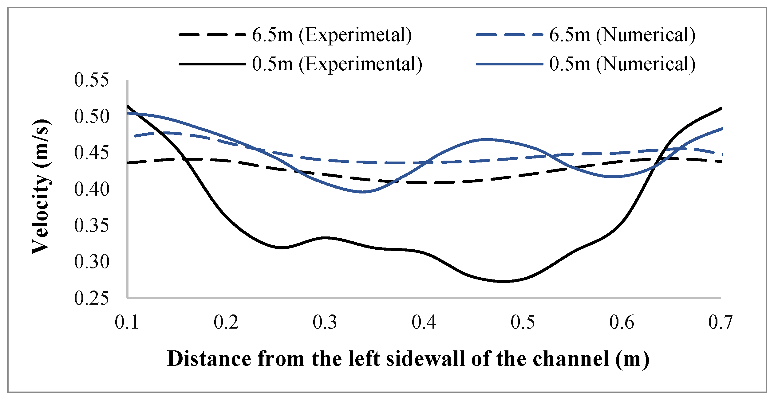
The comparison of numerical and experimental cross-sectional velocity profiles at 0.5 m and 6.5 m (Figure 14) downstream of the turbine reveals a generally consistent trend in the lateral distribution of flow velocities, with notable differences in magnitude and profile steepness. At 0.5 m, the numerical results exhibit higher velocities in the central region of the channel (e.g., 0.35 m to 0.45 m), where experimental data show significantly lower values due to more pronounced wake-induced velocity deficits. This discrepancy is likely attributed to the limitations of steady-state turbulence modeling in capturing complex unsteady wake structures observed in experiments. On the other hand, at 6.5 m, the agreement between the two datasets improves, particularly near the channel center, where velocity differences fall within a margin of ±0.02 m/s in most positions. Both profiles demonstrate wake recovery, yet the numerical solution appears to slightly overpredict velocities near the wake core while underpredicting them near the sidewalls. These observations suggest that while the CFD model captures the general behavior of wake expansion and velocity redistribution, it tends to smooth out the local velocity gradients observed in physical measurements, especially in the near-wake zone. Each velocity profile was measured multiple times (at least three times) at every sampling point, and the standard error values remained low across all measurements, confirming the consistency of the experimental results. The Acoustic Doppler Velocimeter (ADV) was calibrated prior to data collection, and no significant sensor drift was observed throughout the measurement campaign.

The root mean square error (RMSE) between the experimental and numerical mean velocity profiles was calculated as 0.04486, while the mean absolute error (MAE) was found to be 0.03241. These error values suggest a reasonable level of agreement between the two datasets and indicate that the numerical model provides a satisfactory representation of the experimental flow patterns.

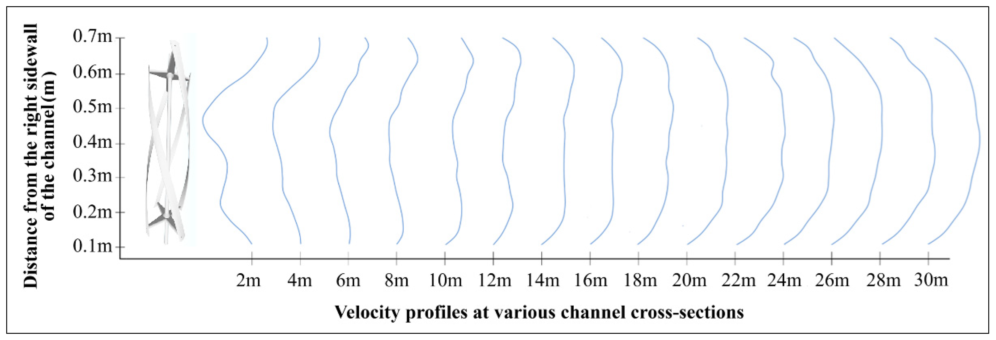
The numerical velocity profiles, at multiple downstream positions ranging from 2 m to 30 m, are given in Figure 15. In the early sections (2–6 m), a noticeable velocity deficit near the mid-depth of the channel indicates the presence of a well-defined wake region. As the flow progresses beyond 10 m, the profiles gradually become more symmetric and smoother, suggesting progressive wake recovery through turbulent mixing and momentum diffusion. By 18–20 m, the velocity curves closely resemble the freestream shape, indicating that the wake has substantially dissipated and the flow has nearly returned to uniform conditions.

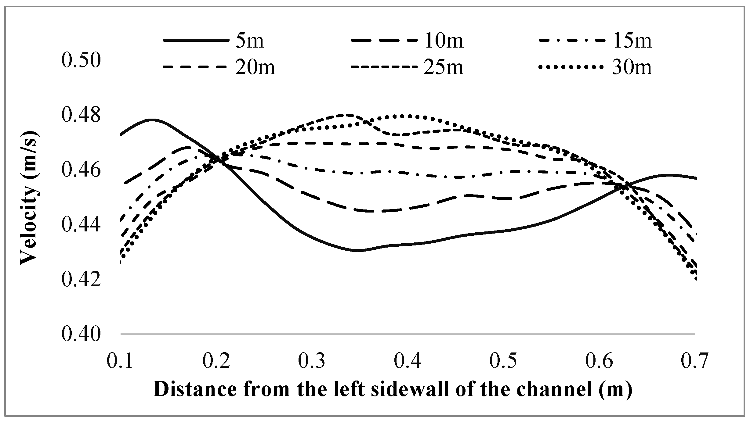
The numerical velocity data measured from 5 m to 30 m downstream of the turbine (Figure 16) reveal the wake recovery dynamics along the longitudinal axis of the channel. In the near-wake region (5–10 m), moderate velocity deficits are still present, particularly at the center of the channel (around 0.35–0.45 m), where velocities remain in the range of 0.43–0.45 m/s. This indicates that although the initial wake deficit has diminished compared to the turbine exit region, flow re-stabilization is still ongoing. Between 15 m and 20 m, the axial velocities gradually increase across the entire width of the channel, with values typically rising above 0.46 m/s, especially in the mid-span zone (0.25–0.45 m). This trend reflects significant momentum recovery and reduction in turbulence intensity in the wake core. Such recovery behavior is critical in determining optimal spacing for turbine arrays, as insufficient wake development can result in power loss and increased structural loading on downstream units. Based on the observed velocity uniformity beyond 18–20 m, this region is suggested as a feasible location for the placement of a second turbine in series.

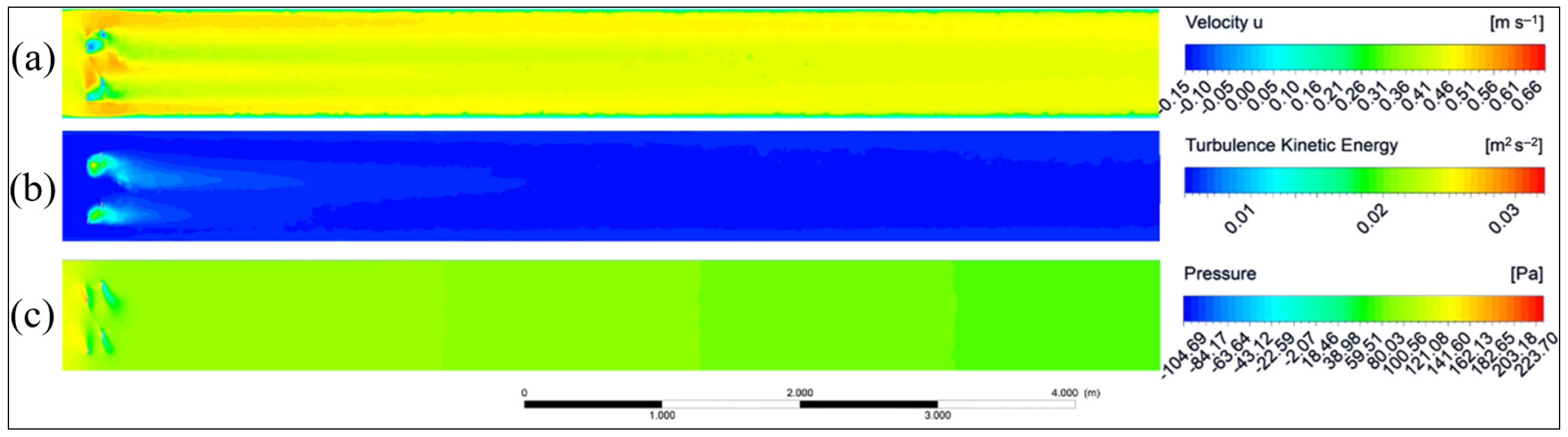
The streamwise evolution of velocity, turbulence kinetic energy (TKE), and pressure counters behind the helical hydrokinetic turbine is given in Figure 17. This is determined according to the distribution of turbulence kinetic energy (TKE) in a 0.80 m wide open water channel, following the operation of two turbines or rotors. High-TKE regions are observed immediately downstream of the turbines, particularly within the first 0.5–1 m, indicating strong wake turbulence and energy dissipation. As the flow progresses, TKE rapidly decreases, and by approximately 2–3 m downstream, the turbulence levels are noticeably lower, suggesting significant wake recovery. Beyond 4 m, TKE values approach background levels, indicating that the wake has largely dissipated and the flow is stabilizing. 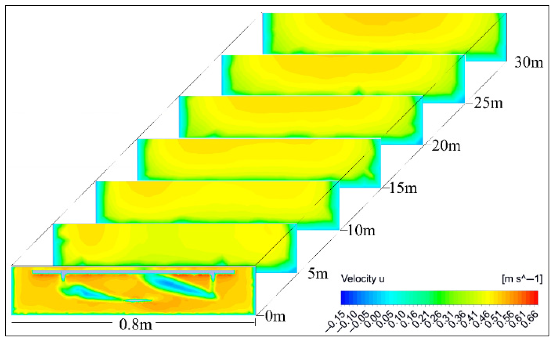Figure 18 illustrates the streamwise velocity distribution downstream of a hydrokinetic turbine, clearly depicting the formation and gradual dissipation of the wake. A substantial velocity deficit is evident within the first 5 m downstream, indicating strong flow disruption due to energy extraction and blade-induced turbulence. Between 5 m and 20 m, the wake undergoes progressive recovery through turbulent mixing and momentum diffusion. Notably, from approximately 18–20 m onward, the velocity field begins to return to near-ambient conditions, suggesting the effective dissipation of the wake. This observation carries important implications for the configuration of hydrokinetic turbine arrays. Positioning downstream turbines within the disturbed wake region at distances shorter than 20 m may result in decreased performance and increased unsteady loading. Therefore, the findings emphasize the importance of maintaining adequate spacing between turbines, with a recommended minimum of 18–20 m, to reduce wake interference and ensure efficient energy extraction in hydrokinetic energy systems.

5. Results

This study presents combined experimental and numerical analysis of the wake characteristics induced by a four-bladed helical hydrokinetic turbine. The experimental campaign was conducted in a recirculating open water channel using an Acoustic Doppler Velocimeter (ADV) to measure velocity profiles at thirteen downstream cross-sections, ranging from 0.5 m to 6.5 m. In parallel, numerical simulations were carried out using ANSYS Fluent with the SST k-ω turbulence model to replicate and compare flow behavior over the same domain.

Between 0.5 and 6.5 m downstream, the experimental results revealed a maximum velocity deficit of approximately 41 percent near the turbine at 0.5 m, which steadily decreased to 5 percent by 6.5 m. In the same range, turbulence intensity values declined from above 50 percent to below 10 percent. The velocity profiles showed clear recovery trends, yet remained asymmetrical, indicating that full flow symmetry had not been achieved within this distance.

The numerical simulation predicted a maximum velocity deficit of 16.6 percent at 0.5 m downstream, decreasing to approximately 4.8 percent at 6.5 m. Turbulence intensity values followed a similar trend, declining from 23 percent to nearly 8 percent within the same section. Although both methods indicated consistent recovery patterns, the numerical results reported lower peak values of velocity deficit and turbulence intensity compared to the experimental findings. However, the similarity in recovery rates confirmed the numerical model’s capacity for reliable wake prediction.

The distances where the velocity deficit ranges between 5% and 10% are generally considered to reprsent the point where the wake effect has ended or can be neglected. In the experimental study, the wake effect was found to be no longer significant at a distance of 5 m downstream of the turbine, whereas numerical results indicated this distance to be approximately 3.5 to 4 m. Similarly, wake dissipation is often identified where the turbulence intensity falls within the 5% to 8% range. Experimental turbulence intensity measurements suggest that the wake effect becomes negligible around 4 m downstream, a finding that is also supported by turbulence kinetic energy calculations from numerical simulations. When considering both numerical and experimental measurements, the wake effect typically dissipates between 3.5 and 5 m downstream of the turbine. For the turbine with a 20 cm rotor diameter, these wake dissipation distances correspond to approximately 17.5 RD to 25 RD, indicating that in serial turbine deployments, turbine spacing should be set within this range.

Analysis of cross-sectional velocity profiles from experimental and numerical data up to 6.5 m downstream of the turbine indicates that, although similar recovery trends are observed, the velocity profiles do not fully normalize within this distance. Extended numerical simulations up to 30 m show that significant flow stabilization and velocity profile normalization occur after approximately 18 to 20 m (90 RD–100 RD) downstream. According to these findings, the distance where the wake effect fully dissipates is approximately between 90 RD and 100 RD, and in the case of serial turbine arrangements, this spacing is recommended between turbines to ensure velocity recovery and maintain turbine efficiency. When only turbulence intensity and velocity deficit are considered, wake dissipation appears to occur within 17.5 RD to 25 RD; however, based on cross-sectional velocity profile normalization this distance should be in the range of 90 RD to 100 RD. The results indicate that, rather than relying solely on turbulence intensity and velocity deficit, it is also important to evaluate the normalization of cross-sectional velocity profiles when assessing wake dissipation, as this offers a clearer indication of full flow recovery.

It should be noted that the results and recommendations provided in this study are limited to the specific laboratory environment, flow conditions, turbine characteristics (such as size, type, and geometry), and simulation parameters utilized. The steady-state turbulence model used in this study provides practical insight into mean wake behavior, but it may not capture all transient or dynamic flow features that could arise under different circumstances. Consequently, the recommended downstream spacing is based on the wake recovery observed for the tested configuration.