Intelligent Optimized Diagnosis for Hydropower Units Based on CEEMDAN Combined with RCMFDE and ISMA-CNN-GRU-Attention

Abstract

This study suggests a hybrid approach that combines improved feature selection and intelligent diagnosis to increase the operational safety and intelligent diagnosis capabilities of hydropower units. In order to handle the vibration data, complete ensemble empirical mode decomposition with adaptive noise (CEEMDAN) is used initially. A novel comprehensive index is constructed by combining the Pearson correlation coefficient, mutual information (MI), and Kullback–Leibler divergence (KLD) to select intrinsic mode functions (IMFs). Next, feature extraction is performed on the selected IMFs using Refined Composite Multiscale Fluctuation Dispersion Entropy (RCMFDE). Then, time and frequency domain features are screened by calculating dispersion and combined with IMF features to build a hybrid feature vector. The vector is then fed into a CNN-GRU-Attention model for intelligent diagnosis. The improved slime mold algorithm (ISMA) is employed for the first time to optimize the hyperparameters of the CNN-GRU-Attention model. The experimental results show that the classification accuracy reaches 96.79% for raw signals and 93.33% for noisy signals, significantly outperforming traditional methods. This study incorporates entropy-based feature extraction, combines hyperparameter optimization with the classification model, and addresses the limitations of single feature selection methods for non-stationary and nonlinear signals. The proposed approach provides an excellent solution for intelligent optimized diagnosis of hydropower units.

1. Introduction

With the growing scale and complexity of water resource systems, maintaining the stable operation of key infrastructure has become increasingly critical. Hydropower generating units serve as crucial actuating components in water resource engineering systems, and their operational status directly affects the safety and efficiency of overall water resources scheduling. Therefore, developing an intelligently optimized diagnostic model is essential. Such a model would enable hydropower units to achieve condition awareness and risk warning at the equipment level, not only improving operational safety and economic efficiency [1], but also providing critical support for basin-scale integrated water resource management and operation decisions. Meanwhile, the proposed intelligently optimized diagnostic model can serve as an optimization tool for maintenance decision-making, supporting predictive maintenance and risk management for sustainable hydropower operation. However, the actual operation of hydropower units is typically influenced by multiple factors such as hydraulic, mechanical, and electromagnetic forces, resulting in complex vibration signals and increased fault identification difficulty. In addition, the strong coupling characteristics of the hydro–mechanical–electrical system [2] lead to significant nonlinearity and non-stationarity [3] in the vibration signals, along with strong background noise. Hence, achieving an efficient and accurate intelligent diagnostic model for hydropower units remains highly challenging.

The intelligent diagnosis of hydropower unit operating states mainly involves key steps such as vibration signal feature processing, feature selection, feature extraction, and vibration pattern recognition. In the following sections, each of these steps is discussed in detail to explain its significance and the methods selected for implementation.

Signal processing methods for vibration signals involve three principal methodologies: time-domain, frequency-domain, and time-frequency analysis [4]. In the time domain, signal properties are quantified using statistical parameters including mean, peak amplitude, root mean square (RMS), and kurtosis. However, it fails to capture periodic information effectively, which may cause biased results. In frequency-domain analysis, the Fourier transform converts signals to spectral representations [5]. This allows the extraction of features such as mean frequency, RMS frequency, and spectral centroid. Nevertheless, this method assumes signal stationarity, limiting its effectiveness for non-stationary signals. Time-frequency analysis simultaneously characterizes temporal and spectral information and commonly employs techniques such as wavelet transform [6], short-time Fourier transform [7], and variational mode decomposition (VMD) [8]. While empirical mode decomposition (EMD) adaptively handles non-stationarity, it is susceptible to boundary artifacts and mode mixing [9]. Although ensemble EMD (EEMD) alleviates mode mixing, it introduces residual noise and modal inconsistency [10]. To further suppress mode mixing, this study adopts complete ensemble empirical mode decomposition with adaptive noise (CEEMDAN) to extract intrinsic mode functions (IMFs) from vibration signals [11].

Previous studies commonly rely on Pearson’s correlation to examine linear interactions between IMFs and the primary vibration signal. For example, Song et al. applied CEEMDAN decomposition and calculated PCCs for each IMF. They retained the top eight IMFs with high correlation (λ > 0.2) and discarded the rest [12]. However, PCC mainly measures linear correlation and cannot effectively capture critical information in nonlinear, non-stationary signals. In contrast, mutual information (MI) [13] reveals nonlinear dependencies, while Kullback–Leibler (KL) divergence quantifies differences in probability distributions between IMFs and the original signal [14], making it suitable for complex signal analysis. To leverage the strengths of different methods and overcome individual limitations, this paper proposes a combined screening strategy. Specifically, PCC, MI, and KL divergence are integrated into a composite index for IMF selection. Meanwhile, time-domain and frequency-domain features are filtered based on their variance, forming a hybrid feature vector set to support subsequent feature extraction.

In intelligent diagnostics, entropy is a key tool for quantifying signal complexity. Traditional entropy methods such as Shannon entropy (ShanEn) [15,16], approximate entropy (ApEn) [17], and sample entropy (SE) [18] are widely used but suffer from low computational efficiency and high noise sensitivity. Dispersion entropy (DE) combines the advantages of sample entropy and symbolic dynamic entropy, offering a novel complexity measure. However, subsequent studies have pointed out that MDE still suffers from several limitations, such as insufficient sensitivity to fluctuation patterns, loss of important signal details due to linear coarse-graining, and increased entropy bias at large scale factors [19]. Building on this, multiscale fluctuation dispersion entropy (MFDE) [20] introduces fluctuation characteristics and multiscale analysis to improve performance over traditional entropy methods. However, MFDE’s fluctuation analysis cannot fully capture complex signal variations, and estimation bias increases with larger scale factors. To address these issues, this research implements refined composite multiscale fluctuation dispersion entropy (RCMFDE), a method that enhances information extraction by integrating refined composite approaches with multiscale fluctuation analysis, demonstrating improved performance.

In the field of intelligent hydropower unit diagnostics, pattern recognition aims to accurately classify various vibration modes. Common methods include extreme learning machine (ELM) [21], support vector machine (SVM) [22], random forest (RF) [23], and deep learning. Notably, deep learning’s multilayer structures can efficiently extract high-level abstract features and have strong generalization ability, fitting the need for high-order nonlinear feature learning in complex systems [24,25]. Convolutional neural networks (CNNs) are effective for spatial feature extraction [26], while gated recurrent units (GRU) offer fewer parameters and faster computation than long short-term memory networks (LSTM) [27,28], making them suitable for real-time fault detection. Additionally, self-attention mechanisms can focus on key features to enhance model performance [29]. Building upon these advantages, this paper proposes a CNN-GRU-Attention model that integrates the spatial feature learning of CNN, the sequence modeling capability of GRU, and the focus mechanism of attention. Furthermore, scientific hyperparameter tuning is crucial for improving model generalization, especially for complex tasks. Conventional manual tuning is time-consuming and inefficient, while swarm intelligence algorithms can effectively address this issue [30], such as particle swarm optimization (PSO) [31], sparrow search algorithm (SSA) [32], and whale optimization algorithm (WOA) [33]. However, these algorithms may suffer from slow convergence and local optima. In comparison, the slime mold algorithm (SMA) mimics the oscillatory foraging behavior of slime molds and demonstrates excellent global search ability, especially for complex nonlinear problems [34]. For instance, Vashishtha et al. applied SMA to optimize ELM parameters, significantly improving defect recognition performance [35]. However, the original SMA is highly sensitive to initial parameter settings and may suffer from slow convergence or local optima in complex tasks. For example, Li et al. [36] mentioned the limitations of SMA and pointed out that it has significant potential for improvement. Therefore, this study develops an improved version of SMA (ISMA), incorporating chaotic mapping and inertia weight adjustment mechanisms. In this study, ISMA is employed for tuning the parameters that govern the CNN-GRU-Attention model, thereby improving its overall effectiveness and stability.

To tackle the challenges of inadequate noise robustness and limited accuracy in feature classification models, this work combines CEEMDAN and RCMFDE for feature extraction, constructs hybrid features via a comprehensive evaluation index, and feeds the hybrid vectors into the ISMA-optimized CNN-GRU-Attention model to achieve precise operational status diagnosis for hydropower units. Comparative experimental results with various diagnostic methods validate the enhanced diagnostic performance and effectiveness of the proposed methodology. This study presents the first known integration of an improved slime mold algorithm (SMA) with a deep hybrid model (CNN-GRU-Attention), specifically optimized for hydropower fault diagnosis. Additionally, the implementation of RCMFDE demonstrates enhanced feature extraction capability under noisy and nonlinear conditions, an aspect that remains underexplored in existing literature.

2. Materials and Methods

2.1. CEEMDAN Algorithm

The complete ensemble empirical mode decomposition with adaptive noise (CEEMDAN) is an improved signal processing method based on the Complementary Ensemble Empirical Mode Decomposition (CEEMD). By introducing adaptive noise and an updated residual signal strategy, it effectively mitigates the problem of mode mixing [37]. Its specific decomposition steps are as follows:

(1) Add Gaussian white noise to the signal $y\left(t\right)$ to obtain $y\left(t\right)+\epsilon {\omega }^j\left(t\right)$. Perform EMD to obtain the first intrinsic mode function (IMF) component:

$${IMF}_1\left(t\right)={\displaystyle \frac{1}{M}}\sum _{j=1}^M{IMF}_1^j\left(t\right)$$

(1)

(2) The residual between the signal y(t) and ${IMF}_1$ is

$$y_1\left(t\right)=y\left(t\right)-{IMF}_1\left(t\right)$$

(2)

(3) Add Gaussian white noise to the residual $y_1\left(t\right)$ and perform EMD to obtain ${IMF}_2$:

$${IMF}_2\left(t\right)={\displaystyle \frac{1}{M}}\sum _{j=1}^M{IMF}_2^j\left(t\right)$$

(3)

(4) Compute the second residual:

$$y_2\left(t\right)=y_1\left(t\right)-{IMF}_2\left(t\right)$$

(4)

(5) The procedure above is iteratively applied until the remaining residual signal cannot be further broken down using EMD. This yields k IMF components, and the final residual is $y_k\left(t\right)$. The original signal $y\left(t\right)$ can then be expressed as

$$y\left(t\right)=\sum _{i=1}^k{IMF}_i+y_k\left(t\right)$$

(5)

2.2. Selection of Mode Decomposition Components

Assuming that the i-th samples of signals X and Y are $x_i$ and $y_i(i=\mathrm{1,2},\dots ,n)$, where n is the number of samples.

The Pearson correlation coefficient $\rho (X,Y)$ is used to reflect the degree of linear correlation between variables [38]. It is defined as

$$\rho \left(X,Y\right)={\displaystyle \frac{\sum _{i=1}^n(x_i-\overline{x})(y_i-\overline{y})}{\sqrt{\sum _{i=1}^n{(x_i-\overline{x})}^2}\sqrt{\sum _{i=1}^n{(y_i-\overline{y})}^2}}}$$

(6)

where $\overline{x }$ and $\overline{y}$ denote the means of signals X and Y, respectively.

However, this method tends to overlook the nonlinear characteristics of vibration signals and has certain limitations. Mutual information (MI) quantifies the statistical relationship between variables exhibiting nonlinear associations. Larger MI values signify a greater level of interdependence and shared information content between signals. The MI between X and Y is calculated as

$$I\left(X;Y\right)=\sum _{y\in Y}\sum _{x\in X}{p}_{XY}\left(x,y\right)\log {\displaystyle \frac{p_{XY}\left(x,y\right)}{p_X\left(x\right)p_Y\left(y\right)}}$$

(7)

where $p_{XY}\left(x,y\right)$ is the joint probability of X and Y, and $p_X\left(x\right)$,${ P}_Y\left(y\right)$ are marginal probabilities. $x\in X$ and $y\in Y$ represent possible values taken by the sample points $x_i$ and $y_i$.

The Kullback–Leibler (KL) divergence evaluates how the probability distribution of an IMF deviates from that of the original signal. A smaller KL divergence indicates greater similarity to the original signal, while a larger value indicates greater dissimilarity. Let the probability distributions of signals X and Y be $p_X\left(x\right)$ and $p_Y\left(y\right)$, respectively. The KL divergence can be mathematically expressed as follows

(1) Define the kernel density function:

$$P_X\left(x\right)={\displaystyle \frac{1}{Nh}}\sum _{i=1}^{n}K({\displaystyle \frac{x_i-x}{h}})$$

(8)

where h is a given positive number, and K is the Gaussian kernel function:

$$K\left(u\right)={\displaystyle \frac{1}{\sqrt{2\pi }}}{e}^{-{\displaystyle \frac{u^2}{2}}}$$

(9)

(2) Similarly, $P_Y\left(x\right)={\displaystyle \frac{1}{Nh}}\sum _{i=1}^{N}K\left({\displaystyle \frac{x-y_i}{h}}\right)$. The KL distances $\delta \left(p_X,p_Y\right)$ and $\delta (p_Y,p_X)$ are then computed as

$$\delta \left(p_X,p_Y\right)=\sum _{x\in X}{P}_X\left(x\right)\log {\displaystyle \frac{P_X\left(x\right)}{Q_Y\left(x\right)}}$$

(10)

(3) Similarly, $\delta \left(p_X,p_Y\right)=\sum _{yϵY}{p}_Y\left(y\right)log{\displaystyle \frac{p_Y\left(y\right)}{p_X\left(y\right)}}$.By substituting the KL distance obtained from Equation (2), the KL divergence is derived as

$$D\left(p_X,p_Y\right)=\delta \left(p_X,p_Y\right)+\delta \left(p_Y,p_X\right)$$

(11)

To address the shortcomings of relying on individual metrics, this study introduces a hybrid evaluation criterion integrating correlation coefficients, mutual information, and KL divergence. This multi-index approach enhances robustness and reduces the impact of noise on screening accuracy. The corresponding equation is

$$E\left(X,Y\right)={\omega }_1\widehat{\rho }\left(X,Y\right)+{\omega }_2\widehat{I}\left(X;Y\right)+{\omega }_3\widehat{D}\left(p_X,p_Y\right)$$

(12)

where ${\omega }_1,{\omega }_2,{\omega }_3$ are weight coefficients. $\widehat{\rho }\left(X,Y\right),\widehat{ I}\left(X;Y\right),$ and $\widehat{D}\left(p_X,p_Y\right)$ are derived through both positive transformation and normalization. To fully utilize the advantages of the three metrics, they are assigned equal contributions in the composite evaluation, i.e., ${\omega }_1={\omega }_2={\omega }_3={\displaystyle \frac{1}{3}}$.

2.3. Refined Composite Multiscale Fluctuation Dispersion Entropy (RCMFDE)

The RCMFDE introduces a refined composite mechanism based on MFDE. Its computation method is as follows:

(1) For a time series $x=\left\{x_1,x_2\dots x_L\right\}$, the k-th coarse-grained time series $\left\{x_{k,1}^{\tau },x_{k,2}^{\tau },\dots \right\}$ is defined as

$$x_{k,j}^{\tau }={\displaystyle \frac{1}{\tau }}\sum _{b=k+\left(j-1\right)\tau }^{k+j\tau -1}{u}_b$$

(13)

where $1\le j<⌊{\displaystyle \frac{L}{\tau }}⌋$,$1\le k\le \tau$.

(2) Compute the average probability of the dispersion pattern π in $x_k^{\tau }$:

$${\overline{p}}^{\tau }\left({\pi }_{v_0{v}_1\dots v_{m-1}}\right)={\displaystyle \frac{1}{\tau }}\sum _{k=1}^{\tau }{p}_k^{\tau }$$

(14)

where ${\overline{p}}_k^{\tau }$ is the probability of each possible dispersion pattern ${\pi }_{v_0{v}_1\dots v_{m-1}}$ with different starting points.

(3) Calculate the Shannon entropy of the average probability of the above dispersion patterns to obtain the RCMFDE:

$$F_{RCMFDE}\left(a,m,c,d,\tau \right)=-\sum _{\pi =1}^{{\left(2c-1\right)}^{m-1}}{\overline{p}}^{\tau }\left({\pi }_{v_0{v}_1\dots v_{m-1}}\right)·\ln \left[{\overline{p}}^{\tau }\left({\pi }_{v_0{v}_1\dots v_{m-1}}\right)\right]$$

(15)

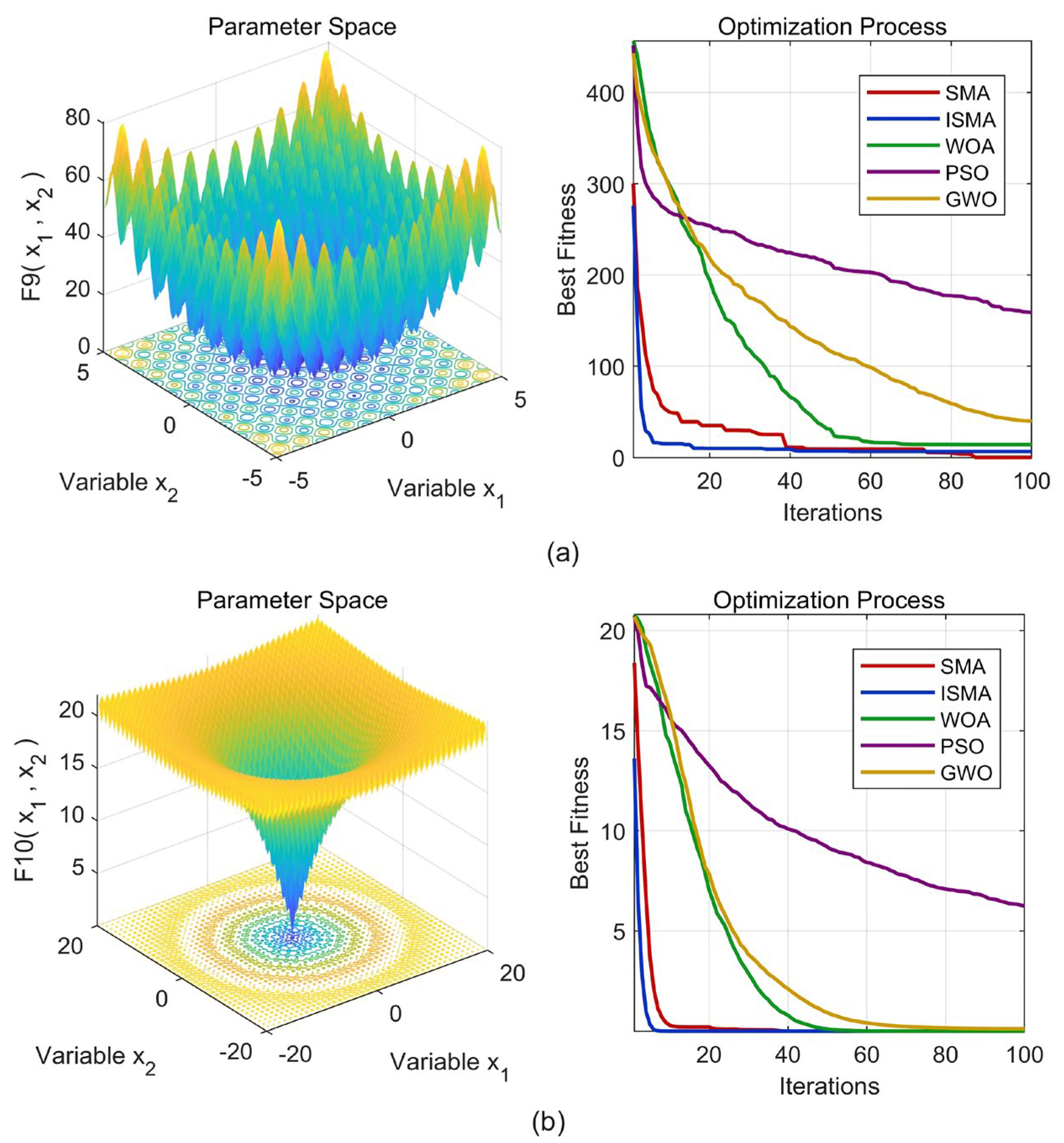
2.4. Establishment of the ISMA Algorithm

As a metaheuristic optimization technique, the slime mold algorithm (SMA) emulates the feeding patterns exhibited by Physarum polycephalum organisms. It adjusts individual positions and search paths dynamically according to the perceived fitness of the environment (i.e., the nutrient amount or food source distribution at the current location). However, the algorithm tends to depend on the initial position and may easily fall into local optima.

To further enhance the search performance of SMA, this paper introduces a Tent chaotic map and an inertia weight mechanism to propose an improved SMA (ISMA).

The traditional SMA generates the initial population using a random distribution. To enhance this process and reduce the risk of getting stuck in local optima within the solution space, the Tent chaotic map is introduced. Its formulation is as follows:

$$x_{n+1}=\left\{\begin{array}{c}2x_n, 0\le x_n<0.5\\ 2\left(1-x_n\right), 0.5\le x_n\le 1\end{array}\right.$$

(16)

where $x_n$ is the current value of the chaotic sequence, $x_{n+1}$ is the next value with $n=\mathrm{0,1},2,\dots ,L-1$, and L specifies the length of the sequence needed to generate the initial population. (L $=$ population size $\times$ number of dimensions).

The adaptive inertia weight is updated in real time according to the distance between the current position of the slime mold individual and its historically best-known position [39]. This allows the algorithm to maintain high exploration capability in the early search stage and enhance local search accuracy when approaching the optimal solution, thereby improving convergence speed and solution precision. The inertia weight at the t-th iteration is defined as

$$\omega \left(t\right)={\omega }_{max}-\left({\omega }_{max}-{\omega }_{min}\right)·{\displaystyle \frac{t}{T}}$$

(17)

where ${\omega }_{max}$ is the maximum inertia weight, ${\omega }_{min}$ is the minimum inertia weight, and T is the maximum number of iterations.

2.5. CNN-GRU-Attention Model

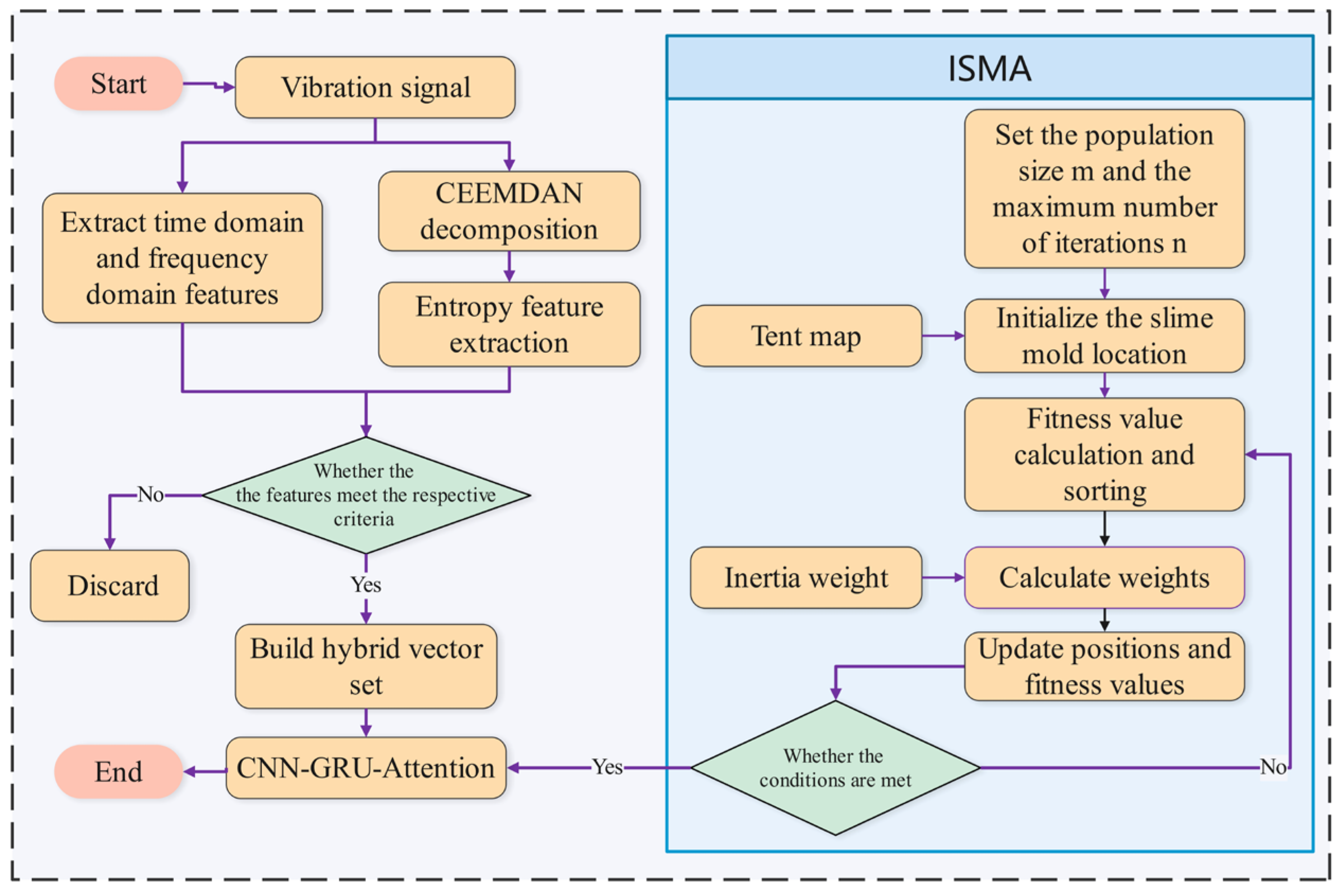
The convolutional neural network (CNN) consists of an input layer, convolutional layers, pooling layers, and fully connected layers [40]. Its expression is as follows:

$$f\left(X_k^l\right)=\sigma \left[\sum _{i=1}^{T}conv\left({\omega }_{ik}^{l-1},r_i^{l-1}\right)+b_k^l\right]$$

(18)

where $X_k^l$ represents the output of the k-th neuron in the l-th layer, $\sigma$ is the ReLU activation function, conv() denotes the convolution operation, ${\omega }_{ik}^{l-1}$ is the convolution kernel weight between the i-th neuron in the (l − 1)-th layer and the k-th neuron, $r_i^{l-1 }$ is the output of the i-th neuron in the (l − 1)-th layer, $b_{k }^l$ is the bias of the k-th neuron in the l-th layer, and T is the number of neurons.

The gated recurrent unit (GRU) introduces gate-controlled recurrence, which reduces computational complexity compared to traditional recurrent neural networks such as LSTM, and effectively alleviates the problems of gradient vanishing and exploding. The formulas are as follows:

$$r_t=\sigma \left(W_r·\left[h_{t-1},x_t\right]+b_r\right)$$

(19)

$$z_t=\sigma \left(W_z·\left[h_{t-1},x_t\right]+b_z\right)$$

(20)

$${\tilde{h}}_t=\tanh \left(W_h·\left[r_t⨀h_{t-1},x_t\right]+b_h\right)$$

(21)

$$h_t=\left(1-z_t\right)⨀h_{t-1}+z_t⨀{\tilde{h}}_t$$

(22)

where $r_t$ is the reset gate output,$z_t$ is the update gate output, $h_{t-1}$ is the previous hidden state, $h_t$ is the current hidden state $\sigma$ id the sigmoid activation function, $W_r{,W}_z,W_h$ are the corresponding weight matrices, $b_r,b_z,b_h$ are the corresponding biases, and $x_t$ is the input at the current time step.

In the intelligent diagnosis of hydropower units, the self-attention mechanism can adaptively assign weights to focus on important feature regions in the signal, thereby improving diagnostic accuracy. Central to self-attention is the transformation of input sequences through linear projections and the calculation of their corresponding attention weights. Given an input matrix $X$, it is subjected to a linear transformation using three distinct weight matrices $W_Q$, $W_k$, and $W_v$ to obtain the query, key, and value matrices as $Q=X{W}_Q$, $K=X{W}_K$, $V=X{W}_V$, respectively. The formula is as follows:

$$Attention\left(Q,K,V\right)=Softmax\left({\displaystyle \frac{Q{K}^T}{\sqrt{d_k}}}\right)V$$

(23)

where $d_k$ is the dimensionality of the key vectors, used as a scaling factor to stabilize gradients during training.

2.6. Proposed Model

In this research, the vibration signals are initially decomposed via CEEMDAN, followed by feature extraction using RCMFDE. The resulting features are then integrated with time-domain and frequency-domain characteristics to create the hybrid feature vector. These samples are partitioned into training and testing sets following a predefined ratio and subsequently input into the CNN-GRU-Attention model for feature classification. Simultaneously, the ISMA is applied to fine-tune the neural network’s parameters. The diagnostic framework is presented in Figure 1.

3. Results and Discussion

3.1. Simulation Experiments

Due to the coupling effects of mechanical, hydraulic, and electrical factors during the operation of hydropower units, conducting a comprehensive study of such systems is relatively challenging. Therefore, existing research often concentrates on specific dynamic behaviors. Among these, the nonlinear dynamic characteristics of rotating machinery systems exert a direct influence on the safety and stability of hydropower operations. In light of this, the present study centers on diagnosing the vibration states of the rotating system to enhance the precision of fault identification.

The rotating machinery test rig, as an experimental platform that simulates large rotating machinery, can replicate various typical fault modes (such as imbalance and misalignment). It offers high repeatability and controllability, providing an important experimental reference for studying the operating state and fault patterns of hydropower unit rotating machinery systems. In this study, the publicly available rotating machinery dataset by Brito et al. is used. This dataset includes experimental data for four typical conditions: normal, imbalance, misalignment, and mechanical looseness [41].

As illustrated in Figure 2, the experimental platform primarily comprises a motor, a frequency converter, a bearing housing, two bearings, two pulleys, a belt, and a rotor (disk). The acceleration signals in the dataset were collected by four accelerometers positioned at different locations, with a sampling rate of 25 kHz. Considering the large scale of the dataset and to balance computational resources with experimental accuracy, only the data from the first accelerometer position (vertical side of the coupling) are used for analysis in this study. There are 420 signals for each condition, with each signal containing 25,000 data points, resulting in a total of 2100 signals per sensor and 8400 signals across the four conditions.

To replicate the complex working conditions of actual hydropower units, noise with a signal-to-noise ratio (SNR) of 2 dB was intentionally introduced to the raw signals. Subsequently, a comparative analysis was conducted to assess the fault state discrimination capability and robustness of the proposed method under low-SNR conditions. A summary of the experimental data samples and their signal characteristics is presented in

Table 1. Data samples and signal characteristics.

State	Sample Length	Number of Samples	Label
Normal	25,000	2100	0
Looseness	25,000	2100	1
Misalignment	25,000	2100	2
Unbalance	25,000	2100	3

.

3.2. CEEMDAN Decomposition

Figure 3 and Figure 4, respectively, show the CEEMDAN decomposition diagrams of four different types of state signals under the pristine signal and the noisy signal (SNR = 2 dB).

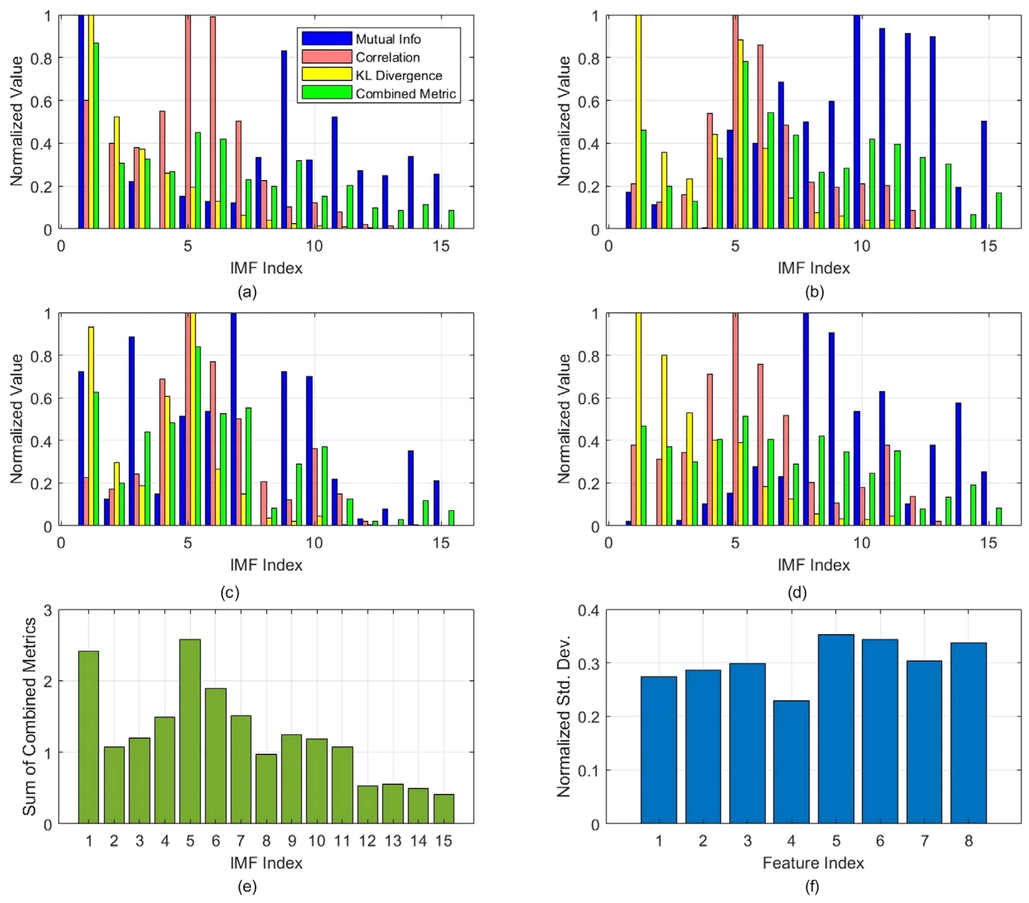
3.3. Constructing the Hybrid Feature Vector Set

Fault diagnosis effectiveness is greatly determined by the performance of feature extraction techniques, which fundamentally governs the precision and trustworthiness of the final diagnostic outcomes. In this study, a comprehensive evaluation system based on correlation coefficient, mutual information, and KL divergence is employed to conduct an in-depth analysis of different types of signals. For the four signal conditions, the top five signals from each condition are first selected and divided into four groups for preliminary feature selection and analysis.

As shown in Figure 5, for each group, the correlation coefficient, mutual information, and KL divergence are evaluated for every intrinsic mode function relative to the source signal, followed by group-wise averaging. These indicators are then normalized and converted to a positive scale. By performing a weighted sum of the normalized values of each evaluation index, a comprehensive evaluation score for each IMF is obtained. The eight IMFs exhibiting superior composite evaluation metrics are identified through ranking analysis to form the preliminary feature collection. These selected IMFs are IMF1, IMF3, IMF4, IMF5, IMF6, IMF7, IMF9, and IMF10.

Time-domain and frequency-domain features serve as a critical component in representing the time distribution and spectral characteristics of signals. In this study, the dispersion degree (i.e., standard deviation) of the feature vectors is used to evaluate the capability of each feature to distinguish between different fault types. By comparing the dispersion levels of various features, time-domain and frequency-domain features exhibiting low variability are eliminated, and the retained features are subjected to normalization. Finally, the three features with the highest dispersion are selected. The analysis indicates that frequency-domain features generally exhibit a higher relative standard deviation compared to time-domain features. Therefore, features numbered 5, 6, and 8 are selected, with dispersion degrees of 0.3530, 0.3442, and 0.3375, respectively. The numbering and statistical characteristics of the time-domain and frequency-domain features are detailed in

Table 2. Decomposition component characteristics.

Group	State
Group 1	Normal
Group 2	Looseness
Group 3	Misalignment
Group 4	Imbalance

and

Table 3. Time-domain and frequency-domain features.

No.	State
1	Kurtosis
2	Peak Value
3	Crest Factor
4	Skewness
5	Mean Frequency
6	Root Mean Square Frequency
7	Frequency Skewness
8	Frequency Kurtosis

and Figure 5.

Finally, the filtered IMF vector set is combined with the selected time-domain and frequency-domain features to form a comprehensive combined feature representation, which is then used for subsequent classification tasks.

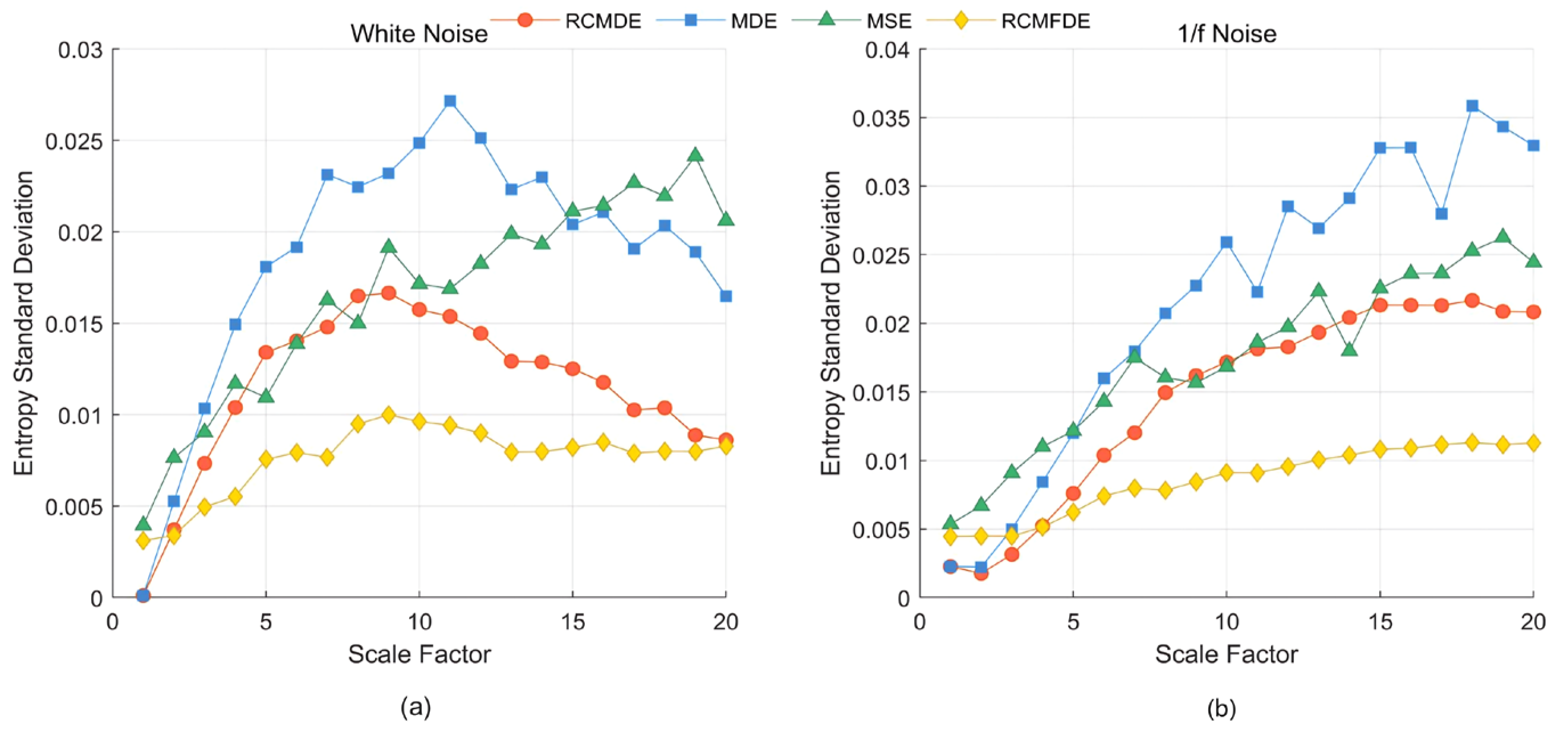
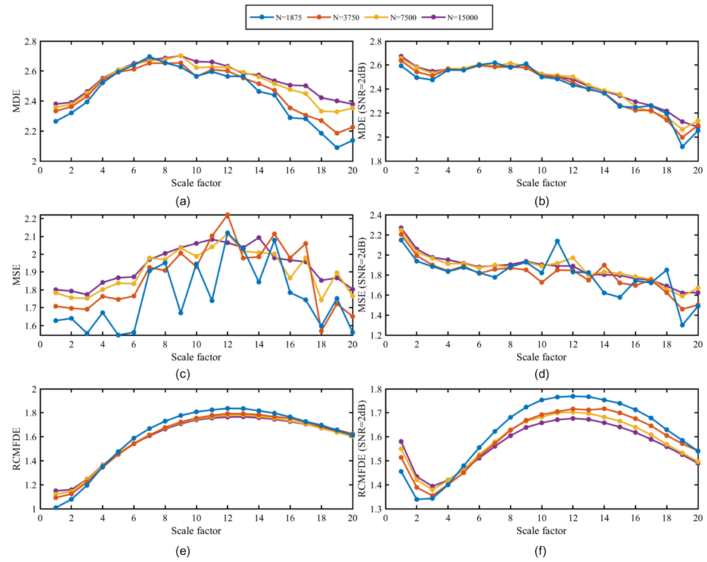
3.4. RCMFDE Performance Analysis

In the field of feature extraction, multiscale entropy methods have become essential tools for analyzing complex signals. In this study, the stability of different entropy methods under various scale factors is systematically investigated, with a focus on their noise resistance and robustness in a low signal-to-noise ratio environment (SNR = 2 dB) and their performance under different signal lengths. The RCMFDE adopted in this paper is implemented based on the MATLAB code provided by Azami et al. on GitHub (commit ID: 6c0da08). Detailed descriptions and implementation can be found in the work of Azami and Escudero [42]. The experimental parameters are set as follows: embedding dimension m = 2; number of classes c = 4 (for RCMDE and MDE); time delay tau = 1; and threshold r = 0.15 (for MSE).

In order to investigate the standard deviation variations in four entropy methods, namely RCMDE (Refined Composite Multiscale Dispersion Entropy), MDE (Multiscale Dispersion Entropy), MSE (Multiscale Sample Entropy), and RCMFDE, under different scale factors, 100 realizations of random white noise and 1/f noise were independently generated and analyzed. Figure 6 presents the results, which reveal that the standard deviation of MSE rises markedly as the scale factor increases. This trend becomes particularly evident when the scale factor surpasses 10, highlighting the metric’s sensitivity to scale variations. In contrast, the standard deviation of RCMFDE exhibits relatively small fluctuations and remains consistently lower than that of the other entropy methods, showing better stability and verifying its superiority in multiscale analysis.

Figure 7 illustrates the variation in entropy values for random signals of different lengths when processed by MDE, MSE, and RCMFDE under varying scale factors. It reveals that the entropy values obtained using MDE and MSE exhibit more pronounced fluctuations as the scale factor increases, particularly at lower signal lengths. In contrast, the RCMFDE results show relatively smoother and more consistent trends across different signal lengths and scale factors. This indicates that RCMFDE is less sensitive to changes in signal length and demonstrates improved stability in multiscale analysis. Furthermore, even in the presence of noise, the entropy curves of RCMFDE remain relatively stable compared to those of MDE and MSE, suggesting that RCMFDE may offer better robustness for entropy-based feature extraction in complex and noisy environments.

As demonstrated in Figure 6 and Figure 7, it can be concluded that RCMFDE can effectively cope with the uncertainties caused by different signal lengths and noise interference, demonstrating high potential for intelligent fault diagnosis and significant advantages in practical applications.

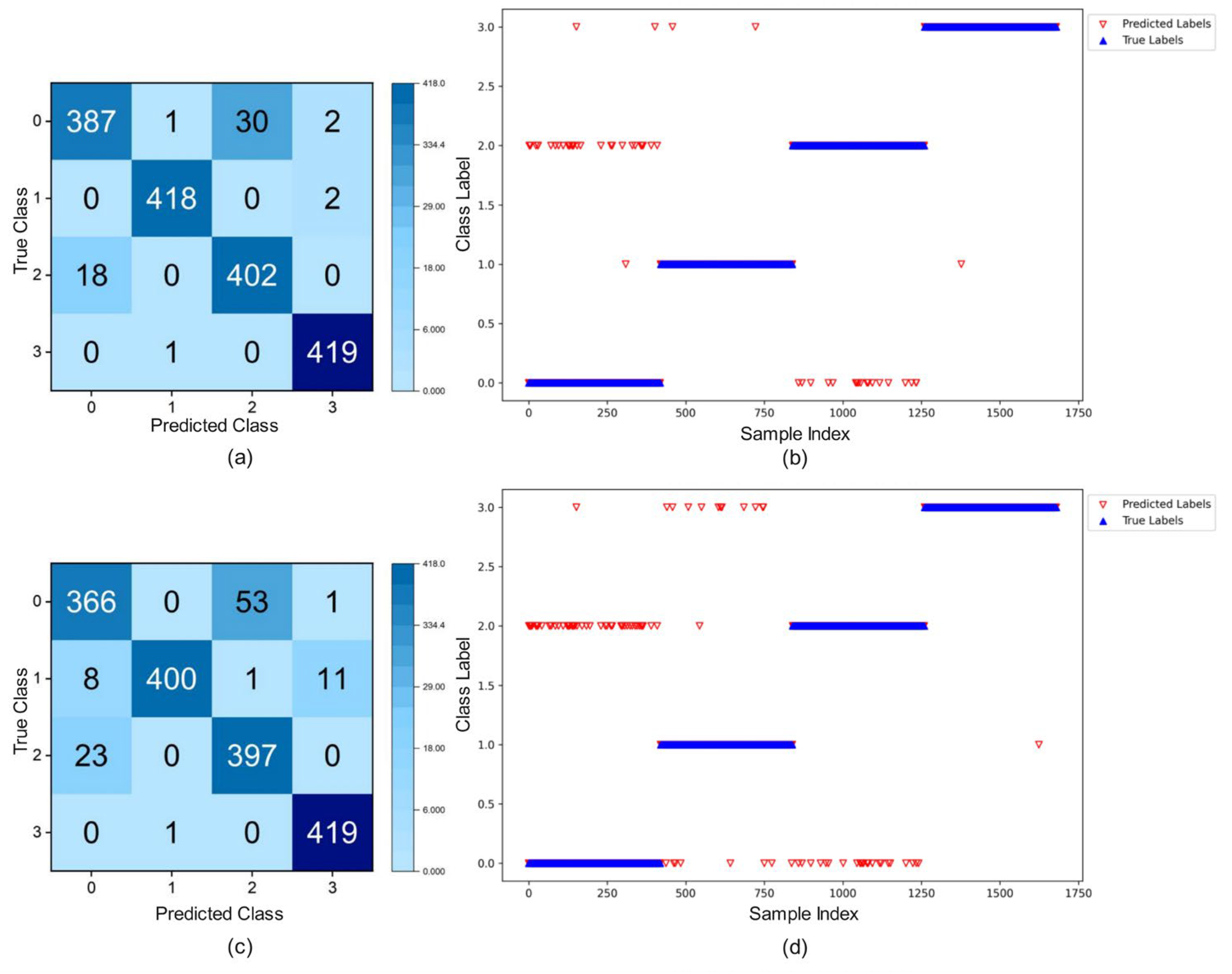
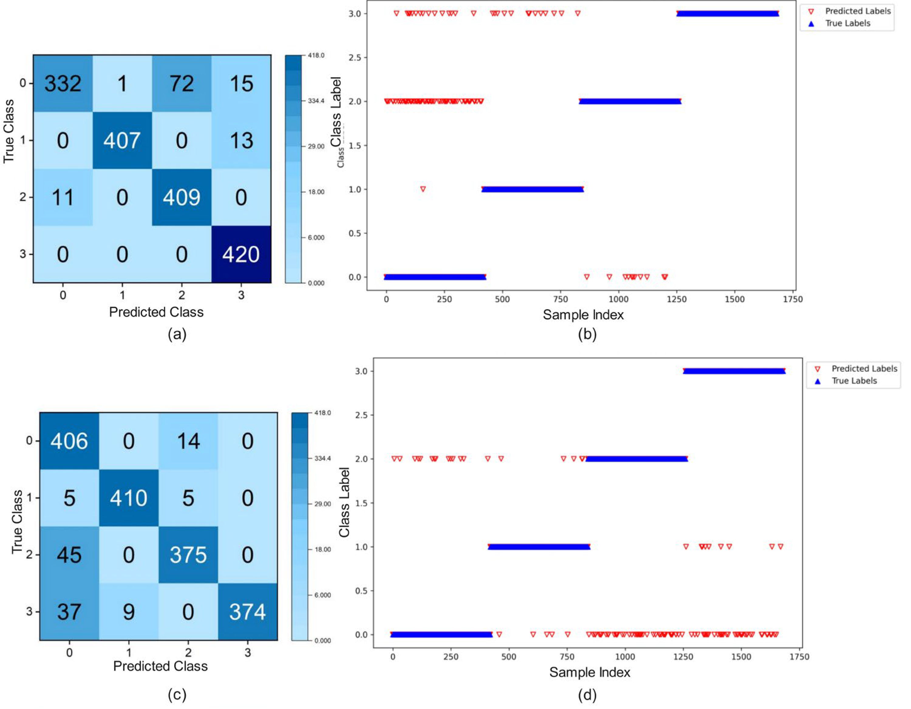
3.5. Intelligent Diagnosis of the ISMA-CNN-GRU-Attention Models

In this study, the feature entropy extracted by MDE, RCMFDE, and MSE is used as input data, which is randomly split into training and testing sets in an 8:2 proportion. The standard SMA and the improved slime mold algorithm (ISMA) are employed to optimize parameters such as the learning rate, the number of GRU neurons, the size of CNN convolution kernels, and the number of training epochs. The number of SMA iterations is set to 50, and the population size is fixed at 20. For RCMFDE, the scale factor is set to 4. The ranges of the parameters are as follows: the learning rate is between 0.00001 and 0.1, the number of GRU neurons is between 32 and 128, the CNN convolution kernel size is between 2 and 5, and the number of training epochs is between 5 and 40. The fitness value is defined as “1—accuracy”. The relationship between the fitness value and the iteration count during parameter optimization is illustrated in Figure 8. The experimental results show that with the position update of SMA, the fitness value gradually decreases. It is observed that ISMA achieves higher convergence precision after approximately 25 iterations and significantly outperforms the standard SMA.

To further verify the convergence performance of the ISMA, the Rastrigin function and the Ackley function are introduced as benchmark functions to compare the optimization performance of ISMA with SMA, WOA, PSO, and GWO, as shown in Figure 9. To improve the reliability of the experiments, each optimization algorithm is executed using 20 different random seeds, and the initial populations are generated randomly. Each experiment runs for 100 iterations, and the mean of the optimization results from 20 trials is calculated. The results indicate that ISMA achieves faster convergence and higher final accuracy compared with SMA. Furthermore, the slime mold algorithm converges more rapidly and performs better than WOA, PSO, and GWO.

(1) The expression of the Rastrigin function is

$$f_9\left(x\right)=\sum _{i=1}^{30}\left[x_i^2-10\cos \left(2\pi x_i\right)+10\right]$$

(24)

where $-5.12\le x_i\le 5.12$,$min\left(f_9\right)=f_9\left(0,\dots ,0\right)=0$.

(2) The expression of the Ackley function is

$$f_{10}\left(x\right)=-20exp\left(-0.2\sqrt{{\displaystyle \frac{1}{30}}\sum _{i=1}^{30}{x}_i^2}\right)-exp\left({\displaystyle \frac{1}{30}}\sum _{i=1}^{30}\cos \left(2\pi x_i\right)\right)+20+c$$

(25)

where $-32\le x_i\le 32$,$min\left(f_{10}\right)=f_{10}\left(0,\dots 0\right)=0$.

Simultaneously, a comprehensive comparison was conducted between the proposed RCMFDE-ISMA-CNN-GRU-Attention method and the RCMFDE-SMA-CNN-GRU-Attention method in terms of classification performance, and the classification effectiveness under noisy signal conditions was also analyzed. Figure 10 and Figure 11 present the classification results and the corresponding confusion matrices based on the RCMFDE feature extraction method combined with SMA optimization.

Table 4. Diagnostic accuracy rates of different models.

NO.	Model	No Noise	SNR = 2 db
1	CEEMDAN-RCMFDE-SMA-CNN-GRU-Attention	94.17%	93.15%
2	CEEMDAN-RCMFDE-ISMA-CNN-GRU-Attention	96.79%	93.33%
3	CEEMDAN-MDE-SMA-CNN-GRU-Attention	90.65%	89.52%
4	CEEMDAN-MDE-ISMA-CNN-GRU-Attention	93.63%	92.02%
5	CEEMDAN-MSE-ISMA-CNN-GRU-Attention	92.20%	—
6	CEEMDAN-RCMFDE-ISMA-CNN-GRU	95.42%	—
7	(Correlation coefficient selection) IMF + CEEMDAN-RCMFDE-ISMA-CNN-GRU-Attention	95.18%	—
8	(KL divergence selection) IMF + CEEMDAN-RCMFDE- ISMA-CNN-GRU-Attention	90.18%	—
9	(MI selection) IMF+CEEMDAN-RCMFDE- ISMA-CNN-GRU-Attention	94.40%
10	IMF (without time-domain and frequency-domain features) + CEEMDAN-RCMFDE-ISMA-CNN-GRU-Attention	94.29%	—
11	CEEMDAN-SVD-PSO-BP [43]	88.99%

Note: The bolded values represent the highest classification accuracy achieved among the compared methods.

shows the classification accuracy of the models using different entropy feature extraction methods and under different noise conditions.

The comparison results demonstrate that the proposed ISMA-CNN-GRU-Attention method achieves the best classification performance, reaching an accuracy of 96.79%. Moreover, employing RCMFDE-derived features generally yields higher classification accuracy compared to that obtained with the MDE approach, which confirms the advantage of RCMFDE in representing multiscale information. In addition, by introducing the ISMA for hyperparameter optimization, the classification accuracy is consistently higher than that obtained using the standard SMA. This indicates that the improved ISMA enhances global search capability through the incorporation of an inertia weight, and the introduced chaotic mapping helps generate higher-quality initial solutions.

To better understand the effectiveness of the feature selection approach, control experiments were carried out using single-indicator-based methods. Specifically, the eight IMF components with the highest correlation coefficients (IMF1, 2, 3, 4, 5, 6, 7, and 10) were selected to construct the feature set for the classification task, achieving a final accuracy of 95.18%. Similarly, selecting the eight IMF components with the highest (normalized) KL divergence values (IMF1, 2, 3, 4, 5, 6, 7, and 8) resulted in an accuracy of 90.18%. Using the top eight IMFs with the highest mutual information (IMF1, 7, 8, 9, 10, 11, 13, and 14) yielded an accuracy of 94.40%. All of these results are lower than the accuracy achieved using the integrated evaluation index method. A comparison with the results from a similar study was made to evaluate the proposed approach’s performance. Specifically, we applied the method presented by Bin et al. to our dataset. Bin et al. used CEEMDAN decomposition, Power Spectrum Energy Distribution for IMF selection [43], followed by PSO-optimized BP for fault diagnosis. The classification accuracy obtained was 88.99%, which is below the 96.79% accuracy in this study.

Considering all the results, the CEEMDAN-RCMFDE-ISMA-CNN-GRU-Attention model based on the integrated evaluation index exhibits improved classification accuracy, demonstrating that the proposed integrated feature selection method can effectively enhance the classification performance and fully verify its applicability in complex signal processing.

4. Conclusions

In this work, an RCMFDE-based approach was employed for feature extraction, and an integrated evaluation metric was used to select key features together with time-domain and frequency-domain characteristics, forming a hybrid feature set for optimizing the CNN-GRU-Attention neural network. By introducing an improved SMA (ISMA), the hyperparameters of the neural network were successfully optimized, and intelligent fault diagnosis was performed using vibration data from a rotating machinery test bench. The experimental results show the following:

(1) RCMFDE outperformed conventional entropy methods, such as MDE and MSE; the proposed RCMFDE method can extract more effective information through refined composite and fluctuation analysis. This highlights its suitability for processing non-stationary and noisy signals encountered in rotating machinery diagnostics.

(2) During feature selection, employing an integrated evaluation criterion enables a more systematic and comprehensive assessment of feature effectiveness than relying on any single indicator such as correlation coefficient, MI, or KL divergence. This effectively selects key variables and reduces the dimensionality of the input data, which may help alleviate the risk of gradient explosion and improve training stability and convergence.

(3) By introducing Tent chaotic mapping and inertia weighting, the ISMA achieves higher classification accuracy and demonstrates improved convergence behavior relative to the standard SMA.

(4) The comparative results of different models indicate that the CEEMDAN-RCMFDE-ISMA feature set selected based on the integrated evaluation index achieves the best performance in neural network training, with significant advantages in both noise resistance and accuracy. Among them, the CNN-GRU-Attention network demonstrates outstanding performance, reaching the highest classification accuracy.

Despite these promising results, some limitations remain. The current study focused on diagnosis under laboratory settings with well-defined fault types and sufficient sample sizes. Its field applicability under variable and noisy real-world environments remains to be validated. Future research should extend validation to more complex and variable operational scenarios, such as real-world hydropower systems with changing loads, multi-fault cases, or unbalanced data distributions. Moreover, in constructing the integrated evaluation index system, this study adopts an equal weight allocation under a simplified model assumption. The impact mechanism of different weighting methods (such as dynamic adaptive weights and static fixed weights) on the evaluation results still needs to be systematically verified according to specific application scenarios. In addition, this study focuses on the intelligent diagnosis of hydropower units from an algorithmic perspective only. Future work will incorporate this algorithm into physical modeling frameworks to improve the interpretability of diagnostic outcomes and strengthen their applicability in real-world scenarios.

In this study, the proposed diagnostic framework was developed under an idealized operating scenario, with a primary focus on improving diagnostic accuracy, as misdiagnosis in hydropower systems can lead to direct economic losses and operational risks. While considerable efforts have been made to design a comprehensive and high-performing intelligent diagnostic solution, the model’s real-time performance remains an open challenge for future research. Furthermore, the interpretability of the model remains limited, as it is difficult to explain which specific features or signal patterns the model relies on to make its diagnostic decisions. This limitation may hinder practical deployment in real-world scenarios that require transparent decision-making and traceability. It is expected that the results, limitations, and future directions presented in this study will contribute to enhancing the adaptability of the proposed method. Such contributions may support the development of more intelligent, transparent, and deployable diagnostic systems for the hydropower industry.

References

1. Hu, C.; Zhang, Z.; Li, C.; Leng, M.; Wang, Z.; Wan, X.; Chen, C. A state of the art in digital twin for intelligent fault diagnosis. Adv. Eng. Inform. 2025, 63, 102963. [Google Scholar] [CrossRef]
2. Wang, Z.; Zhao, H.; Lu, Q.; Wu, T. Improved non-dominated Sorting Genetic Algorithm III for Efficient of Multi-bjective Cascade Reservoirs Scheduling under Different Hydrological Conditions. J. Hydrol. 2025, 656, 132998. [Google Scholar] [CrossRef]
3. Guy, T.B.; Todros, K. Blind separation of noisy piecewise-stationary mixtures via probability measure transform. Signal Process. 2023, 208, 108967. [Google Scholar] [CrossRef]
4. Yao, Z.; Wang, Z.; Huang, J.; Xu, N.; Cui, X.; Wu, J. Interpretable prediction, classification and regulation of water quality: A case study of Poyang Lake, China. Sci. Total Environ. 2024, 951, 175407. [Google Scholar] [CrossRef]
5. Bai, Y.; Cheng, W.; Wen, W.; Liu, Y. Application of Time-Frequency Analysis in Rotating Machinery Fault Diagnosis. Shock Vib. 2023, 2023, 9878228. [Google Scholar] [CrossRef]
6. Yan, R.; Shang, Z.; Xu, H.; Wen, J.; Zhao, Z.; Chen, X.; Gao, R.X. Wavelet transform for rotary machine fault diagnosis:10 years revisited. Mech. Syst. Signal Process. 2023, 200, 110545. [Google Scholar] [CrossRef]
7. Li, Y.; Wang, Z.; Liu, S. Enhance carbon emission prediction using bidirectional long short-term memory model based on text-based and data-driven multimodal information fusion. J. Clean. Prod. 2024, 471, 143301. [Google Scholar] [CrossRef]
8. Sun, B.; Li, H.; Wang, J.; Lv, S.; Ma, Z. Differential time-frequency mode decomposition and its application in rotating machinery fault diagnosis. Mech. Syst. Signal Process. 2025, 229, 112571. [Google Scholar] [CrossRef]
9. Zhang, Y.; Li, C.; Jiang, Y.; Sun, L.; Zhao, R.; Yan, K.; Wang, W. Accurate prediction of water quality in urban drainage network with integrated EMD-LSTM model. J. Clean. Prod. 2022, 354, 131724. [Google Scholar] [CrossRef]
10. Zhou, H.; Chen, W.; Shen, C.; Cheng, L.; Xia, M. Intelligent machine fault diagnosis with effective denoising using EEMD-ICA-FuzzyEn and CNN. Int. J. Prod. Res. 2022, 61, 8252–8264. [Google Scholar] [CrossRef]
11. Tan, R.; Hu, Y.; Wang, Z. A multi-source data-driven model of lake water level based on variational modal decomposition and external factors with optimized bi-directional long short-term memory neural network. Environ. Modell. Softw. 2023, 167, 105766. [Google Scholar] [CrossRef]
12. Song, S.; Zhang, S.; Dong, W.; Zhang, X.; Ma, W. A new hybrid method for bearing fault diagnosis based on CEEMDAN and ACPSO-BP neural network. J. Mech. Sci. Technol. 2023, 37, 5597–5606. [Google Scholar] [CrossRef]
13. Ni, L.; Gu, W.; Zhou, T.; Hao, P.; Jiang, J. Leak aperture recognition of natural gas pipeline based on variational mode decomposition and mutual information. Measurement 2025, 242, 116017. [Google Scholar] [CrossRef]
14. Dong, L.; Chen, Z.; Hua, R.; Hu, S.; Fan, C.; Xiao, X. Research on diagnosis method of centrifugal pump rotor faults based on IPSO-VMD and RVM. Nucl. Eng. Technol. 2023, 55, 827–838. [Google Scholar] [CrossRef]
15. Shannon, C.E. A mathematical theory of communication. Bell Syst. Technol. J. 1948, 27, 379–423. [Google Scholar] [CrossRef]
16. Yao, Z.; Wang, Z.; Wu, T.; Lu, W. A hybrid data-driven deep learning prediction framework for lake water level based on the fusion of meteorological and hydrological multi-source data. Nat. Resour. Res. 2024, 33, 163–190. [Google Scholar] [CrossRef]
17. Dou, C.; Lin, J.; Guo, L. A Novel Feature for Fault Classification of Rotating Machinery: Ternary Approximate Entropy for Original, Shuffle and Surrogate Data. Machines 2023, 11, 172. [Google Scholar] [CrossRef]
18. Richman, J.S.; Moorman, J.R. Physiological time-series analysis using approximate entropy and sample entropy. Am. J. Physiol. Heart Circ. Physiol. 2000, 278, H2039–H2049. [Google Scholar] [CrossRef]
19. Wang, Z.; Li, G.; Yao, L.; Qi, X.; Zhang, J. Data-driven fault diagnosis for wind turbines using modified multiscale fluctuation dispersion entropy and cosine pairwise-constrained supervised manifold mapping. Knowl. Based Syst. 2021, 228, 107276. [Google Scholar] [CrossRef]
20. Azami, H.; Arnold, S.E.; Sanei, S.; Chang, Z.; Sapiro, G.; Escudero, J.; Zhou, X.; Huang, S. Multiscale fluctuation-based dispersion entropy and its applications to neurological diseases. IEEE Access 2019, 7, 68718–68733. [Google Scholar] [CrossRef]
21. Wang, B.; Wang, Z.; Yao, Z. Enhancing carbon price point-interval multi-step-ahead prediction using a hybrid framework of autoformer and extreme learning machine with multi-factors. Expert Syst. Appl. 2025, 270, 126467. [Google Scholar] [CrossRef]
22. Wang, Z.; Yao, L.; Cai, Y. Rolling bearing fault diagnosis using generalized refined composite multiscale sample entropy and optimized support vector machine. Measurement 2020, 156, 107574. [Google Scholar] [CrossRef]
23. Guo, Z.; Du, W.; Li, C.; Guo, X.; Liu, Z. Fault diagnosis of rotating machinery with high-dimensional imbalance samples based on wavelet random forest. Measurement 2025, 248, 116936. [Google Scholar] [CrossRef]
24. Cui, W.; Meng, G.; Wang, A.; Zhang, X.; Ding, J. Application of rotating machinery fault diagnosis based on deep learning. Shock Vib. 2021, 2021, 3083190. [Google Scholar] [CrossRef]
25. Szalai, J.; Mózes, F.E. Intelligent digital signal processing and feature extraction methods. In New Approaches in Intelligent Image Analysis; Kountchev, R., Nakamatsu, K., Eds.; Intelligent Systems Reference Library; Springer: Cham, Switzerland, 2016; Volume 108, pp. 59–91. [Google Scholar] [CrossRef]
26. Jiao, J.; Zhao, M.; Lin, J.; Liang, K. A comprehensive review on convolutional neural network in machine fault diagnosis. Neurocomputing 2020, 417, 36–63. [Google Scholar] [CrossRef]
27. Li, X.; Guo, Y.; Xiao, B.; Jing, Q.; Yun, Z. Stability and safety study of pumped storage units based on time-shifted multi-scale cosine similarity entropy. J. Energy Storage 2024, 95, 112611. [Google Scholar] [CrossRef]
28. Gao, S.; Huang, Y.; Zhang, S.; Han, J.; Wang, G.; Zhang, M.; Lin, Q. Short-term runoff prediction with GRU and LSTM networks without requiring time step optimization during sample generation. J. Hydrol. 2020, 589, 125188. [Google Scholar] [CrossRef]
29. Zheng, Y.; Li, J.; Zhu, T.; Li, J. Experimental and MPM modelling of widened levee failure under the combined effect of heavy rainfall and high riverine water levels. Comput. Geotech. 2025, 184, 107259. [Google Scholar] [CrossRef]
30. Czako, Z.; Sebestyen, G.; Hangan, A. AutomaticAI—A hybrid approach for automatic artificial intelligence algorithm selection and hyperparameter tuning. Expert Syst. Appl. 2021, 182, 115225. [Google Scholar] [CrossRef]
31. Huan, S. A novel interval decomposition correlation particle swarm optimization-extreme learning machine model for short-term and long-term water quality prediction. J. Hydrol. 2023, 625, 130034. [Google Scholar] [CrossRef]
32. Xue, J.; Shen, B. A novel swarm intelligence optimization approach: Sparrow search algorithm. Syst. Sci. Control Eng. 2020, 8, 22–34. [Google Scholar] [CrossRef]
33. Wang, B.; Qiu, W.; Hu, X.; Wang, W. A rolling bearing fault diagnosis technique based on fined-grained multi-scale symbolic entropy and whale optimization algorithm-MSVM. Nonlinear Dyn. 2024, 112, 4209–4225. [Google Scholar] [CrossRef]
34. Liang, C.; Guan, M. Effects of urban drainage inlet layout on surface flood dynamics and discharge. J. Hydrol. 2024, 632, 130890. [Google Scholar] [CrossRef]
35. Vashishtha, G.; Chauhan, S.; Singh, M.; Kumar, R. Bearing defect identification by swarm decomposition considering permutation entropy measure and opposition-based slime mould algorithm. Measurement 2021, 178, 109389. [Google Scholar] [CrossRef]
36. Li, Y.; Wang, X.; Yuan, Q.; Shen, N. HKTSMA: An Improved Slime Mould Algorithm Based on Multiple Adaptive Strategies for Engineering Optimization Problems. KSCE J. Civ. Eng. 2024, 28, 4436–4456. [Google Scholar] [CrossRef]
37. Yao, D.; Chen, S.; Dong, S.; Qin, J. Modeling abrupt changes in mine water inflow trends: A CEEMDAN-based multi-model prediction approach. J. Clean. Prod. 2024, 439, 140809. [Google Scholar] [CrossRef]
38. Gong, H.; Li, Y.; Zhang, J.; Zhang, B.; Wang, X. A new filter feature selection algorithm for classification task by ensembling pearson correlation coefficient and mutual information. Eng. Appl. Artif. Intell. 2024, 131, 107865. [Google Scholar] [CrossRef]
39. Yu, C.; Heidari, A.A.; Xue, X.; Zhang, L.; Chen, H.; Chen, W. Boosting quantum rotation gate embedded slime mould algorithm. Expert Syst. Appl. 2021, 181, 115082. [Google Scholar] [CrossRef]
40. Cao, H.; Shao, H.; Zhong, X.; Deng, Q.; Yang, X.; Xuan, J. Unsupervised domain-share CNN for machine fault transfer diagnosis from steady speeds to time-varying speeds. J. Manuf. Syst. 2022, 62, 186–198. [Google Scholar] [CrossRef]
41. Brito, L.; Susto, G.A.; Brito, J.N.; Duarte, M. Mechanical faults in rotating machinery dataset (normal, unbalance, misalignment, looseness). Mendeley Data 2023, V3. [Google Scholar] [CrossRef]
42. Azami, H.; Escudero, J. Amplitude- and fluctuation-based dispersion entropy. Entropy 2018, 20, 210. [Google Scholar] [CrossRef] [PubMed]
43. Bin, L.; Rongsheng, Z.; Qian, H.; Yongyong, Z.; Qiang, F.; Xiuli, W. Fault diagnosis of horizontal centrifugal pump orifice ring wear and blade fracture based on complete ensemble empirical mode decomposition with adaptive noise-singular value decomposition algorithm. J. Vib. Control 2024, 30, 5228–5236. [Google Scholar] [CrossRef]
Figure 1. Diagnostic model proposed in this study.
Water 17 02125 g001
Figure 2. Schematic diagram of the experimental setup in this study.
Water 17 02125 g002
Figure 3. CEEMDAN decomposition results of vibration signals under different states. (a) Normal. (b) Looseness. (c) Misalignment. (d) Imbalance.
Water 17 02125 g003
Figure 4. CEEMDAN decomposition results of noisy vibration signals under different states. (a) Normal. (b) Looseness. (c) Misalignment. (d) Imbalance.
Water 17 02125 g004
Figure 5. Statistical analysis of time-domain and frequency-domain features in this study. (a) Group 1 indicator value. (b) Group 2 indicator value. (c) Group 3 indicator value. (d) Group 4 indicator value. (e) Aggregated evaluation metric per IMF index. (f) Standard deviations of time-domain and frequency-domain features.
Water 17 02125 g005
Figure 6. Standard deviation variations in RCMDE, MDE, MSE, and RCMFDE across scale factors for white noise and 1/f noise. (a) Entropy standard deviation for white noise. (b) Entropy standard deviation for 1/f noise.
Water 17 02125 g006
Figure 7. Entropy value changes in MDE, MSE, and RCMFDE for original and noise-added signals under different signal lengths. (a) MDE entropy. (b) MDE entropy (with noise). (c) MSE entropy. (d) MSE entropy (with noise). (e) RCMFDE. (f) RCMFDE (with noise).
Water 17 02125 g007
Figure 8. Intelligent diagnostic model fitness curve.
Water 17 02125 g008
Figure 9. Optimization iteration fitness curve. (a) Generalized Rastrigin’s function. (b) Ackley’s function.
Water 17 02125 g009
Figure 10. Classification results of the original signals. (a) RCMFDE-ISMA-CNN-GRU-Attention confusion matrix. (b) RCMFDE-ISMA-CNN-GRU-Attention classification status. (c) RCMFDE-SMA-CNN-GRU-Attention confusion matrix. (d) RCMFDE-SMA-CNN-GRU-Attention classification status.
Water 17 02125 g010
Figure 11. Classification results of signals with SNR = 2 dB noise. (a) RCMFDE-ISMA-CNN-GRU-Attention confusion matrix. (b) RCMFDE-ISMA-CNN-GRU-Attention classification status. (c) RCMFDE-SMA-CNN-GRU-Attention confusion matrix. (d) RCMFDE-SMA-CNN-GRU-Attention classification status.
Water 17 02125 g011