Application of Empirical Mode Decomposition to Land Surface Temperature Projection Under a Changing Climate

Abstract

This study takes the daily temperature series of Taipei City as an example and proposes a data projection method based on Empirical Mode Decomposition (EMD), which effectively resolves the challenge of modeling non-stationary sequences. According to the daily mean temperature records from 1971 to 2023, Taipei has experienced an average warming rate of 0.02 °C per year. After applying EMD, the data were decomposed into 12 intrinsic mode functions (IMFs) and one residual trend. Among them, IMF5, with a period of 352 days (approximately one year), contributes 78% of the total energy, representing the dominant climatic cycle component. In this study, daily temperatures were categorized into five thermal levels: Cold (<12 °C), Cool (12–18 °C), Moderate (18–27 °C), Warm (27–32 °C), and Hot (>32 °C). In addition, using a 5-year moving process based on the annual EMD results, the IMFs and residuals were recombined to generate 390,625 synthetic sequences per year. Results show that the monthly mean temperatures of each year’s simulations closely match the observations, capturing the non-stationary characteristics of temperature variations. The overall classification accuracy of simulated versus observed daily temperature categories ranges from 60% to 71%, with an average of 65.1%. In summary, the EMD combined with the 5-year moving process developed in this study demonstrates a helpful data projection approach with effective reconstruction of periodic structures and stable simulation accuracy. It offers practical value for reconstructing urban climate variability, conducting risk assessments, and analyzing long-term warming trends. Moreover, it serves as a vital tool for modeling non-stationary climate data and supporting future projections.

1. Introduction

As the impacts of global climate change become increasingly pronounced, long-term trends and short-term anomalous fluctuations in regional air temperature have emerged as central concerns in climate research and environmental management [1]. Urban areas are particularly affected. The urban heat island effect, driven by land development, energy use, and high population density, adds layers of complexity and non-stationarity to temperature dynamics [2]. In northern Taiwan’s high-density metropolis of Taipei, daily temperature records over recent decades reveal a clear warming trend alongside multi-scale oscillatory features, indicating that the urban climate system is shaped by interacting factors and exhibits pronounced nonlinearity and non-stationarity [3].

Traditional temperature analysis and forecasting methods such as autoregressive integrated moving average (ARIMA) models and Fourier transforms perform well under stationary conditions but face limitations when applied to long-term climate data that contain significant trends and abrupt changes [4]. These approaches typically assume stationarity, preventing them from effectively identifying or decomposing long-term shifts, nonlinear structures, and multi-scale components within raw time series. Moreover, rising temperatures have important implications for the hydrological cycle. Higher air temperatures accelerate evapotranspiration, reducing soil moisture and surface water availability [5]. This can intensify drought risk during dry seasons and reduce baseflow in urban rivers, particularly in densely populated regions such as Taipei. Warmer conditions also lead to increased atmospheric water demand, further depleting soil moisture reserves and challenging agricultural irrigation management, especially in regions dependent on rainfall rather than regulated reservoirs [6]. In Taiwan, where orographic precipitation dominates, this imbalance can lead to both prolonged dry spells and sudden flash floods.

The sensitivity of hydrological systems to temperature variation is further reflected in the decoupling of rainfall and runoff relationships. As noted by Wang and Hejazi (2011) [7], higher temperatures modify runoff efficiency in temperate zones. Although snowmelt is not a concern in Taipei’s subtropical setting, increased air temperature in low-elevation regions still affects streamflow timing by altering antecedent soil moisture conditions and storm-runoff conversion rates. These temperature-induced shifts in hydrological response necessitate adaptive models that reflect evolving climate baselines.

Increased atmospheric energy also enhances the intensity and variability of convective precipitation. Studies such as Trenberth et al. (2003) have shown that warmer temperatures lead to a more vigorous hydrological cycle, characterized by an increase in heavy rainfall events, even in the absence of significant changes in total annual precipitation [8]. In Taiwan, Lin et al. (2020) reported that urban warming has altered seasonal precipitation distribution and shortened the duration of wet spells, contributing to both water scarcity and flood management challenges [9]. Additionally, research by Huang et al. (2024) [10] on southern China, a region climatologically similar to northern Taiwan, demonstrated that enhanced surface heating increases low-level moisture convergence and convective instability, thereby intensifying hourly rainfall extremes. This suggests that urban temperature trends play a direct role in reshaping local rainfall structures. Furthermore, Lenderink and Van Meijgaard (2008) found that sub-hourly precipitation intensity may increase at rates greater than expected from thermodynamic scaling under urban warming scenarios, a concern that also applies to Taipei’s high-density settings [11].

These nonlinear impacts of temperature on the water cycle highlight the need for integrated, multi-scale tools capable of disentangling overlapping trends and fluctuations in hydrometeorological records. The empirical complexity of these changes, ranging from shifts in precipitation timing to altered drought and flood dynamics, makes traditional linear trend extraction methods increasingly insufficient. For urban climate systems such as Taipei, where temperature-driven feedbacks affect multiple components of the hydrosphere, analytical tools must reflect this interconnected variability. Consequently, strongly non-stationary, periodic urban temperature records like those from Taipei demand adaptive, multi-scale analytical tools.

Empirical Mode Decomposition (EMD), introduced by Huang et al. in 1998, is a data-driven time-series decomposition method specifically designed to analyze nonlinear, non-stationary signals [12]. Through an iterative sifting process, EMD decomposes the original series into a set of Intrinsic Mode Functions (IMFs) and a residual trend component, each IMF corresponding to a well-defined frequency range with clear physical meaning [13]. This decomposition enables researchers to separate and quantify variability at different scales, including daily weather fluctuations, mid-term cyclical structures, and long-term warming trends, and thus perform more insightful simulations and trend forecasts.

EMD has been widely applied in climate variability and hydrological analysis, particularly for nonlinear and non-stationary meteorological and environmental data. In rainfall trend detection, for example, EMD can effectively isolate short-term weather disturbances from long-term precipitation changes, clarifying wet and dry year patterns [14]. For drought monitoring, EMD reveals hidden periodicities in soil moisture and precipitation indices. When combined with the Standardized Precipitation Index (SPI) and vegetation indicators, it facilitates long-term drought risk assessments.

In recent years, EMD has been integrated with various statistical and machine-learning models. Support vector regression (SVR) has been combined with EMD to forecast seasonal rainfall and temperature [15], and long short-term memory (Temperature M) networks have been coupled with EMD to address long-range dependencies and capture complex temporal patterns. These hybrid approaches have outperformed traditional models in tasks ranging from urban temperature prediction to extreme climate event warning and reservoir storage estimation.

Our laboratory has likewise explored EMD-based forecasting for non-stationary climate data. Huang and Lee (2023) [16] applied EMD method to analyze daily sea surface temperature (SST) data for estimating typhoon occurrences. The focus area of the study was 5° N~25° N and 110° E~170° E. The study demonstrated the effectiveness of combining EMD synthesis with statistical regression analysis to evaluate typhoon frequency [16]. Chang et al. (2024) generated El Niño and La Niña occurrence probabilities by resampling IMF components from sea surface temperature time series and computing corresponding ONI distributions, successfully replicating the timing and intensity of major ENSO events [17].

2. Material and Method

2.1. Data Collection

Daily land surface temperature data for this study were obtained from the Taipei Observatory (Station ID: 466920) operated by the Central Weather Administration (CWA) [18]. These records are accessible via the CWA’s Climate Data Open Platform (https://codis.cwa.gov.tw/StationData; accessed on 16 September 2024) [19]. Situated in northern Taiwan, the Taipei Observatory serves as a representative urban station and has long provided accurate daily meteorological observations [20]. We extracted the daily mean temperature series from 1971 through 2023 which spanning 53 years and over 19,000 daily entries, as the primary dataset for analyzing climate variability and trends in the Taipei metropolitan area.

2.2. Variation in Land Surface Temperature

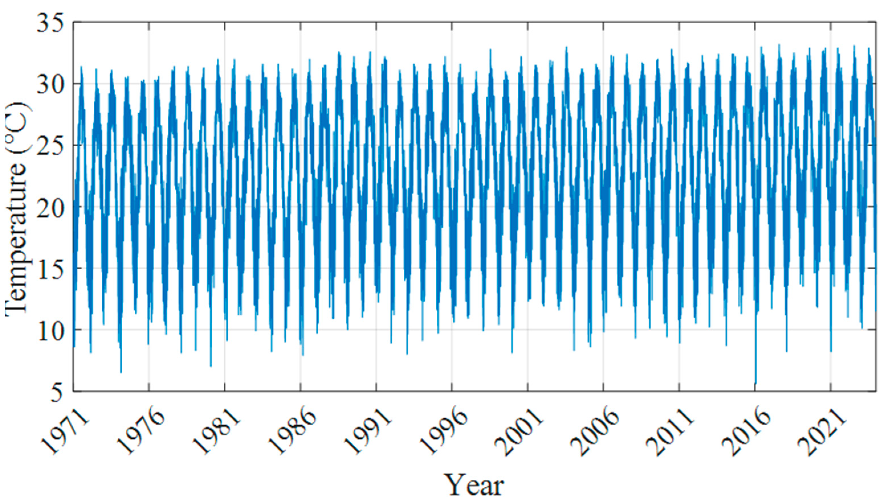
This section analyzes daily, monthly, and annual scales of temperature at the Taipei Observatory (Station 466920) using records from 1 January 1971 to 31 December 2023, accompanied by figures illustrating long-term trends. Figure 1 presents the daily mean temperature over 1971–2023: winter (January–February) averages predominantly range between 10 and 20 °C, while summer (July–August) averages concentrate around 25–30 °C. Since the 1990s, days above 31 °C have become noticeably more frequent in summer, and days below 11 °C have steadily declined in winter. A linear trend overlay indicates a gradual increase in daily mean temperature of approximately 0.02 °C per year (totaling over 2 °C) underscoring a clear long-term warming of Taipei’s climate.

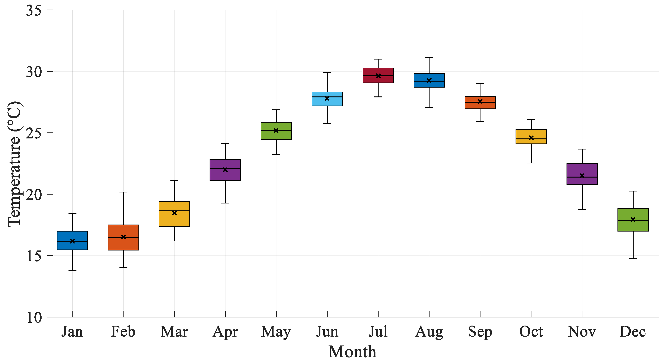
Figure 2 and Figure 3 present statistical characteristics at the monthly and annual scales, respectively. Figure 2 shows boxplots for each month from 1971 to 2023: January and February medians lie around 16–17 °C; March at approximately 18 °C; April through June rising from 20 °C up to 28 °C; July through September holding steady between 27 °C and 28 °C; and October through December declining back to 16–24 °C. Between the 1970s and the present, both medians and quartile boundaries have shifted unmistakably upward, most markedly in late spring (March–May) and peak summer (June–August).

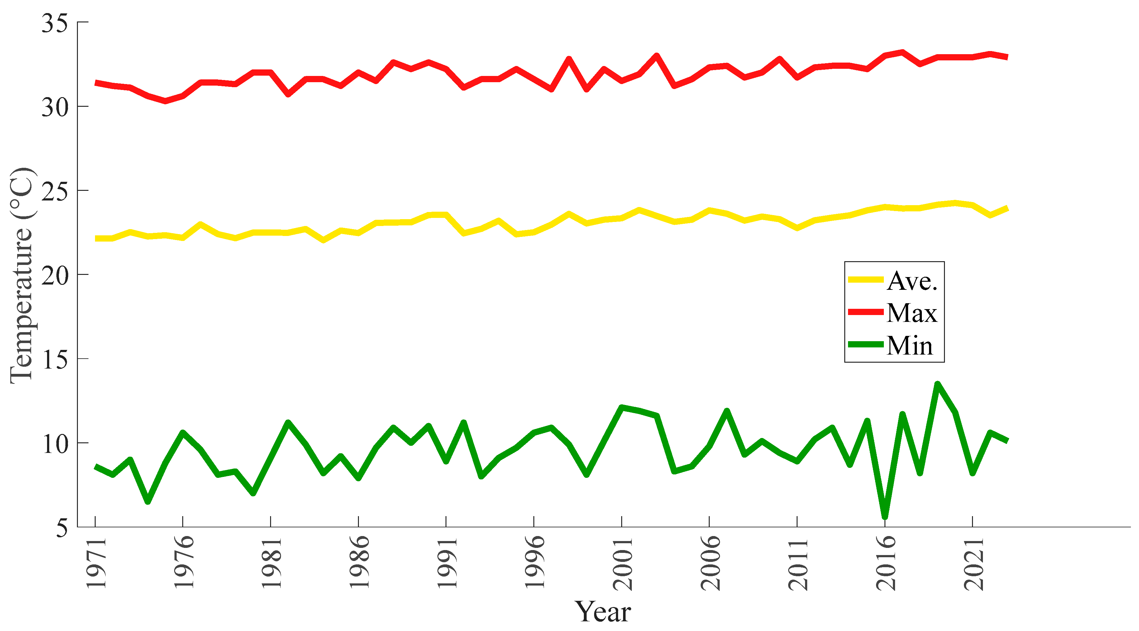
Figure 3 traces the annual mean, maximum, and minimum temperatures over the same period. The mean increased from about 22.1 °C in 1971 to roughly 24.0 °C in 2023, an average rise of 0.04 °C per year. Simultaneously, maximum temperatures climbed from 31.0 °C to 33.2 °C and minimums from 8.5 °C to 10.2 °C. Since the mid-1980s, the gap between daily highs and lows has been narrowing, indicating that summer highs have warmed slightly more than winter lows, reflecting a seasonally variable warming effect.

Figure 4 divides the twelve months into four seasonal segments: January–March (spring), April–June (early summer), July–September (peak summer), and October–December (autumn–winter). It also links each month’s daily temperatures across all years into continuous curves. In spring, the January daily range shifted from roughly 10–28 °C in 1971 to 12–30 °C in 2023, with February and March showing similar upward trends: minima rose from about 12 °C to 14–16 °C, and maxima from about 26 °C to nearly 30 °C. In early summer, April 1 moved from approximately 18 °C in 1971 to 20 °C in 2023, while June 30 climbed from about 30 °C to 32 °C; the reduced spread indicates a more concentrated late-spring warm period [21]. Peak summer curves for July–September show a shift from 24 to 30 °C in 1971 to above 28–32 °C in 2023, with days exceeding 33 °C becoming far more common. In autumn–winter, October 1 rose from about 21 °C in 1971 to 22–23 °C in 2023, and December 31 from about 15 °C to 17–18 °C, while minima climbed from 8 to 10 °C to 10–12 °C, marking a lifted late-year baseline. Together, these seasonal plots not only reveal a synchronized upward shift in monthly baselines but also allow clear comparison of high-low temperature changes for the same month across different decades.

In summary, the combined figures indicate a steady warming trend in Taipei from 1971 to 2023 at an average rate of approximately 0.02 °C per year, with increasingly convergent medians and reduced amplitude in late spring and peak summer, and a particularly marked rise in winter minima that has led to a significant decrease in extreme cold events. While the seasonal cycle persists, its baseline has shifted upward, causing daily mean temperatures across all seasons to be substantially higher than in past decades. These changes reflect the combined effects of urban warming and the heat island phenomenon, offering valuable insights for urban climate adaptation, public health protection, and updates to energy and building regulation models. Future work could incorporate additional meteorological variables such as humidity and wind speed or employ high-resolution simulations to investigate Taipei’s localized microclimate changes, thereby enhancing the precision of policy development and scientific research.

2.3. Brief Overview of Empirical Mode Decomposition

In Empirical Mode Decomposition (EMD) analysis, each Intrinsic Mode Function (IMF) must satisfy two key conditions: (1) the number of extrema (local maxima and minima) and the number of zero crossings in the entire dataset must be equal or differ by at most one; (2) at any point in time, the mean of the upper envelope (defined by the local maxima) and the lower envelope (defined by the local minima) must be zero. These requirements ensure that the extracted IMFs adhere to the basic assumptions underlying the decomposition process.

EMD is straightforward to implement in MATLAB (R2024b). If mode mixing occurs, when a single IMF contains signals of widely disparate scales, the Ensemble Empirical Mode Decomposition (EEMD) method proposed by Wu and Huang can be applied to resolve it. In essence, the original temperature series Temperature (t) can be represented as the sum of $p$ IMF and a residual trend $r\left(t\right)$:

$$\mathrm{T}\mathrm{e}\mathrm{m}\mathrm{p}\mathrm{e}\mathrm{r}\mathrm{a}\mathrm{t}\mathrm{u}\mathrm{r}\mathrm{e}\left(t\right)=\sum _{i=1}^p{\mathrm{I}\mathrm{M}\mathrm{F}}_i\left(t\right)+r\left(t\right)\forall t$$

(1)

The number of IMFs, $p$, is approximately $\lfloor {log}_{2}n\rfloor -1$, where n denotes the sample size. The resulting residual $r\left(t\right)$ is a monotonic function, or at most has a single extremum, reflecting the underlying trend in daily temperatures.

2.4. Conceptual Framework for Land Surface Temperature Data Synthesis

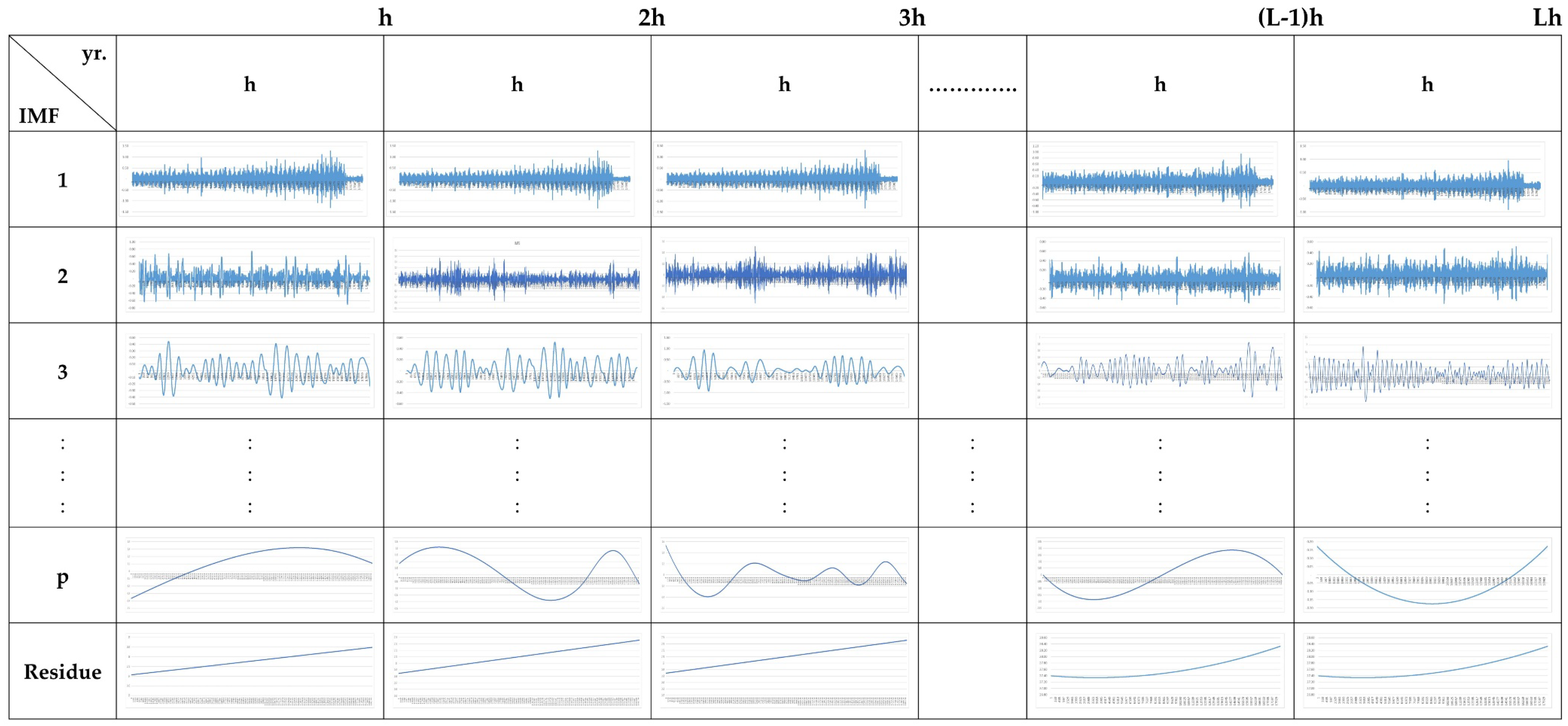
Figure 5 illustrates the approach for synthesizing land surface temperature (Temperature) data. Given a daily mean temperature record spanning L × h years, the series is first divided into L contiguous segments, each of length h years. For one-year reconstructions, one sets h = 1, thereby splitting the full record into L annual segments. Each h-year segment is then subjected to Empirical Mode Decomposition (EMD), yielding p Intrinsic Mode Functions (IMFs) and a residual trend r(t). Because the p IMFs and the residual encapsulate that year’s multi-scale oscillations and baseline change, permuting these components among different years enables the construction of numerous synthetic temperature sequences.

Specifically, when each annual segment is decomposed into $p$ IMFs plus one residual, the total number of possible synthetic sequences created by permuting these components across $L$ years is approximately $L^{p+1}\hspace{0.17em}$, where the exponent $p+1$ represents the $p$ IMFs and the single residual. For one-year synthesis, we set $h=1$, yielding $L$ independent annual segments; by recombining the IMFs and residuals from different years, up to $L^{p+1}\hspace{0.17em}$ distinct daily mean temperature series can be generated.

In practical implementation, the first step is to determine an appropriate value of $L$ for the one-year synthesis using statistical methods such as the autocorrelation function (ACF) or the Mann–Kendall test [22]. Generally, if the autocorrelation analysis indicates significant persistence and memory within the annual temperature series, one chooses a multi-year base to preserve the time-dependency structure; conversely, if inter-annual correlation is weak, $L$ may be set equal to the total number of observed years to increase the diversity of synthetic sequences [23]. Furthermore, one must consider the computational feasibility of $L^{(p+1)}$: if both $p$ and $L$ are large, the number of combinations may become excessive and exceed processing or storage capacity, necessitating a reduction in $L$ or a manual selection of dominant frequency bands to lower $p$.

In summary, the process for synthesizing one-year land surface temperature data consists of the following steps:

• Choose the overall observation length L × 1 years and partition the data into L independent annual segments;
• Apply EMD to each annual segment, decomposing that year’s daily mean temperature series into p IMFs and one residual;
• Determine the value of L based on autocorrelation analysis or prior experience;
• Randomly or systematically recombine the p IMFs and residuals from the L annual segments to generate a new one-year daily mean temperature series;
• Repeat step 4 to produce the required number of synthetic annual series and then perform statistical testing and model validation as needed.

This synthesis framework can flexibly generate multiple one-year land surface temperature datasets that retain the original temporal structure while exhibiting annual-scale variability, making it highly useful for climate studies that lack continuous long-term observations or require large ensembles of simulated samples.

2.5. Temperature Classification

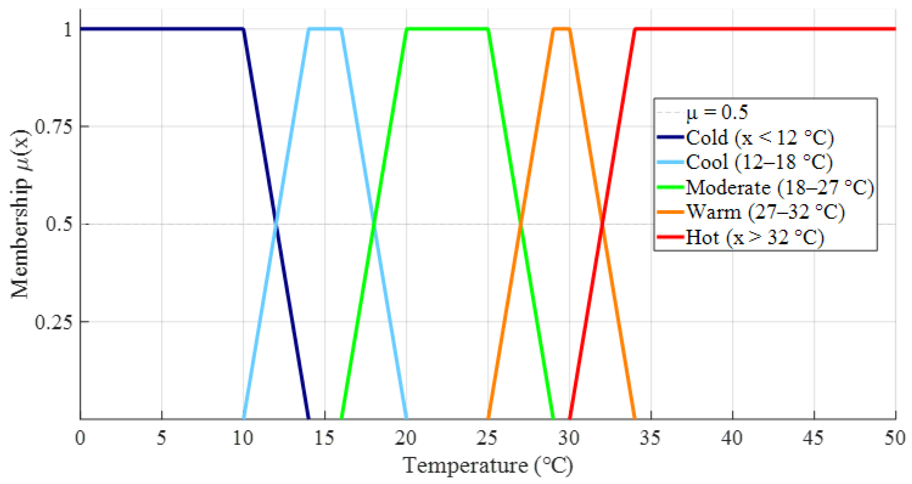
In this study, daily mean temperatures at the Taipei Observatory are classified into five levels: “Cold” (<12 °C), “Cool” (12–18 °C), “Moderate” (18–27 °C), “Warm” (27–32 °C), and “Hot” (>32 °C). These categories are represented by triangular membership functions (see Figure 6). A membership degree µ(x) = 0.5 marks the transition point between two adjacent levels [24], with exact boundaries at 12 °C, 18 °C, 27 °C, and 32 °C. In practice, each historical daily temperature is input into the five membership functions, and if μi(x) ≥ 0.5, the day is assigned to level i; if μ(x) equals exactly 0.5, it is treated as a critical boundary value. This classification approach combines the clarity of fixed thresholds with the flexibility of fuzzy transitions, accurately capturing Taipei’s seasonal progression from “Cold” through “Hot”, and providing a standardized reference for comparing synthetic or forecasted series against observed distributions.

3. Result and Discussion

3.1. Land Temperature Classification Results

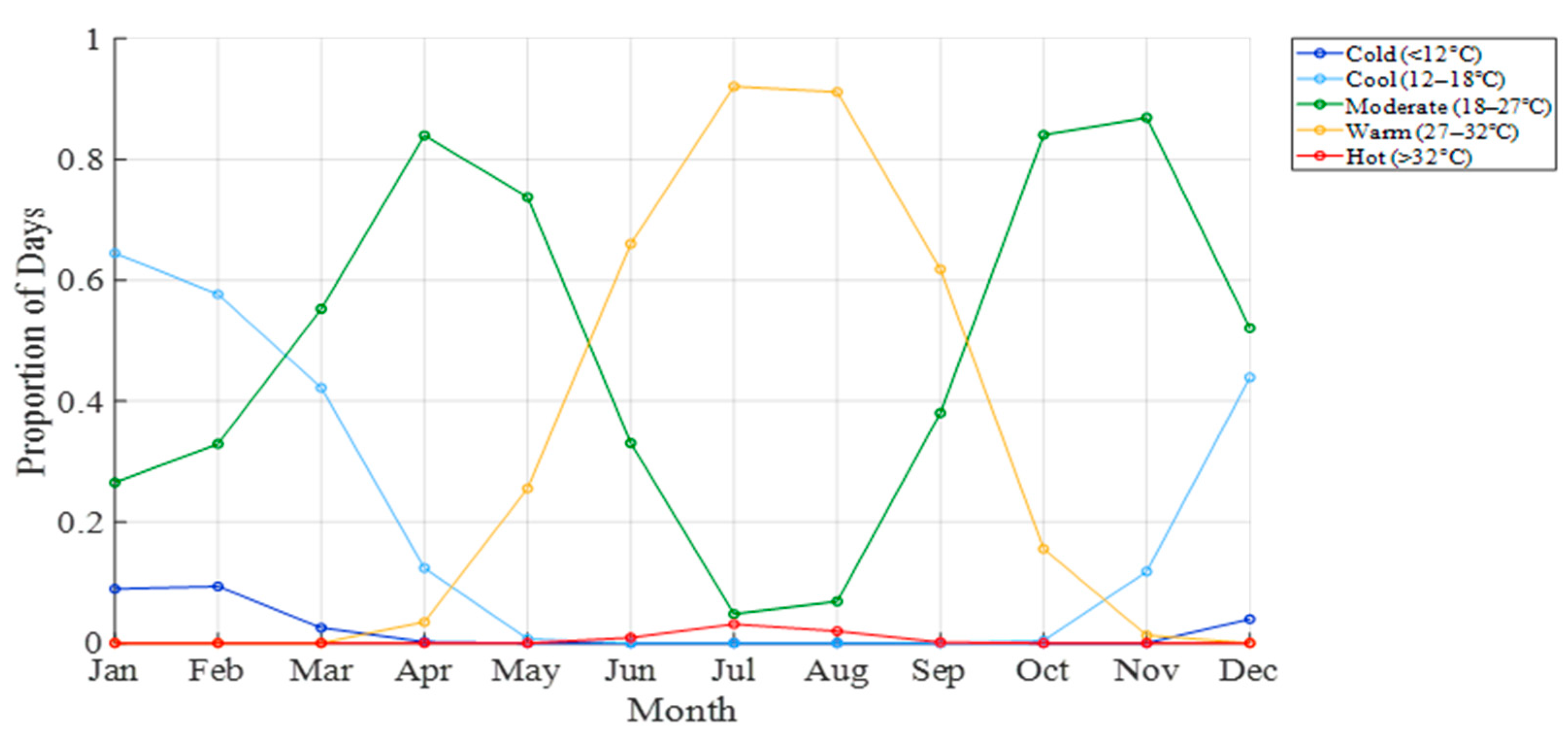
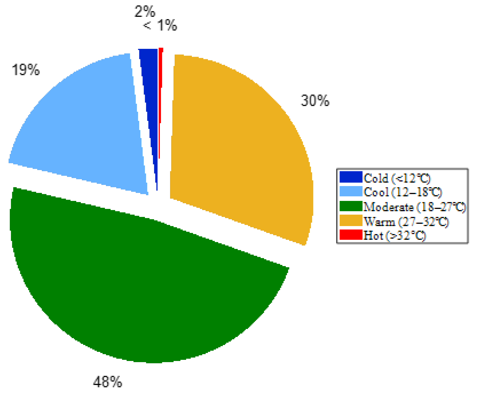
In analyzing the cumulative five-level classification of daily mean temperatures at the Taipei Observatory from 1971 to 2023, we first adopt the five categories: “Cold” (<12 °C), “Cool” (12–18 °C), “Moderate” (18–27 °C), “Warm” (27–32 °C), and “Hot” (>32 °C), as indicated by the legend in Figure 7. Considering the overall distribution (see the pie chart legend in Figure 8), nearly half of all days (about 48%) fall within the “Moderate” range, approximately 30% are “Warm,” 19% “Cool,” and only 2% and 1% are “Cold” and “Hot”, respectively. This demonstrates that over the past fifty years in Taipei, extremely low winter temperatures have been relatively rare, and although days above 32 °C do occur in midsummer, the vast majority of days remain between 18 °C and 32 °C.

When examined, on a monthly basis, the curves in Figure 7 show that the “Cool” category (light blue) peaks in January and February at roughly 65% and 58%, then drops sharply to about 42% in March and near zero thereafter. The “Moderate” category (dark green) rises from March, reaching about 75% in April and May. After June, “Moderate” declines rapidly while the “Warm” category (tan) begins at about 66% in June and climbs to 92% and 91% in July and August, indicating that over ninety percent of midsummer days lie between 27 °C and 32 °C. In September, “Warm” remains around 62%, but falls to approximately 15% in October as “Moderate” rebounds to about 38%. From November onward, “Cool” and “Moderate” both increase again, with “Cool” around 44% and “Moderate” around 52% in December.

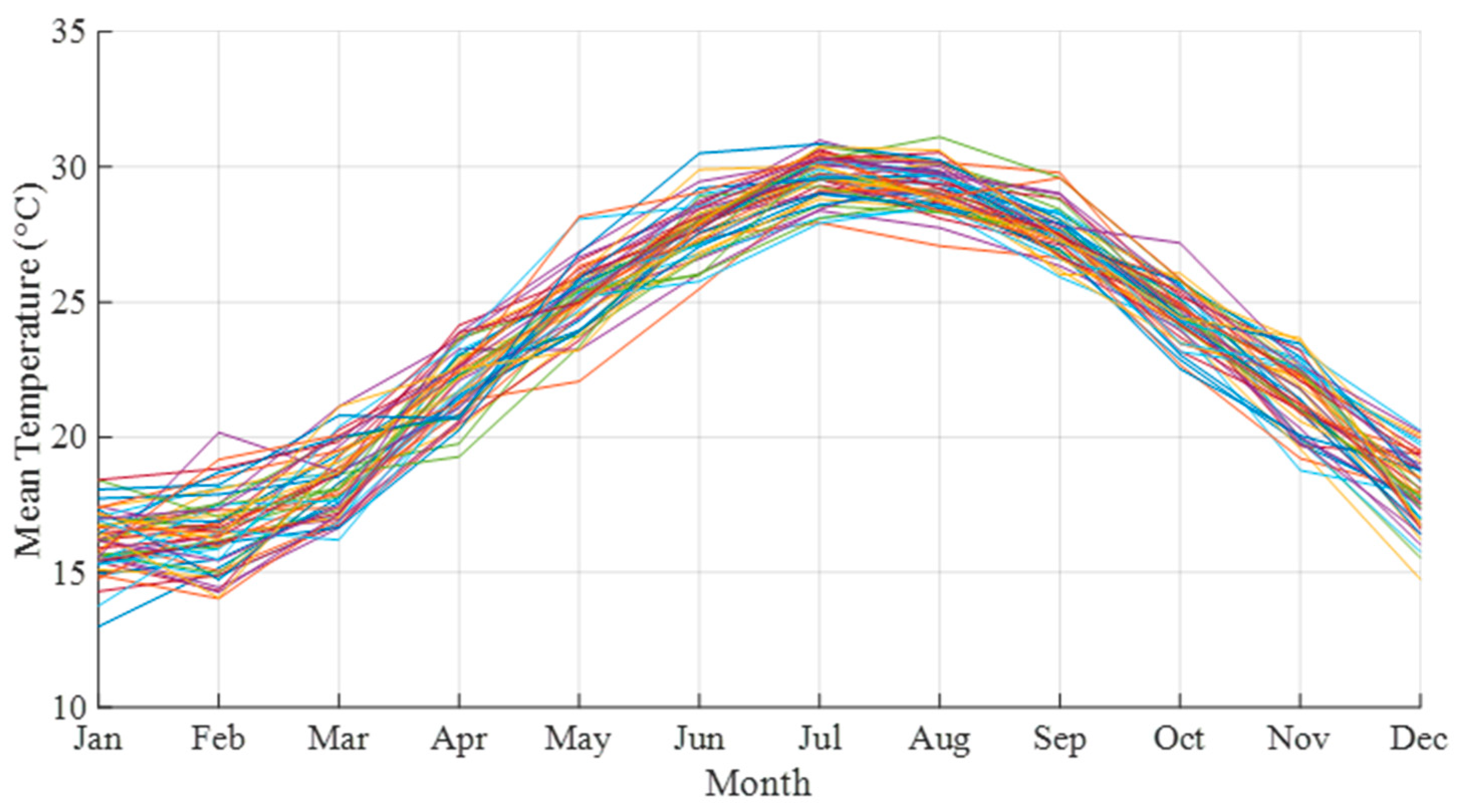
Figure 9 summarizes the monthly mean temperatures for each year from 1971 to 2023. All annual curves display a characteristic single-peak pattern: roughly 15–18 °C in January, rising to about 30 °C in July and August, then falling back to around 14–17 °C in December. Although individual years vary slightly in amplitude and phase, the overall shape remains consistent, with the curves of the past two decades shifted upward relative to those of the 1970s. For example, July’s mean temperature has risen from approximately 29 °C to 30–31 °C in recent years, and December from about 15 °C to around 17 °C. This upward shift across all months reflects the combined influences of global warming and urbanization on Taipei’s monthly average temperatures.

In summary, between 1971 and 2023, the proportion of days classified as “Cold” and “Cool” has steadily declined, “Warm” days in midsummer have significantly increased, and although “Moderate” remains the most common category, its relative share has contracted compared to earlier decades. These results not only corroborate the observed rise in annual average temperatures but also illustrate historical changes in the frequency of extreme cold-spell and heat-wave events. For future data synthesis or short-term forecasting, one can reference the historical proportions shown in Figure 7 and classify model outputs using the same five levels to evaluate the model’s ability to reproduce observed distributions across seasons and temperature categories.

3.2. Characteristics of EMD

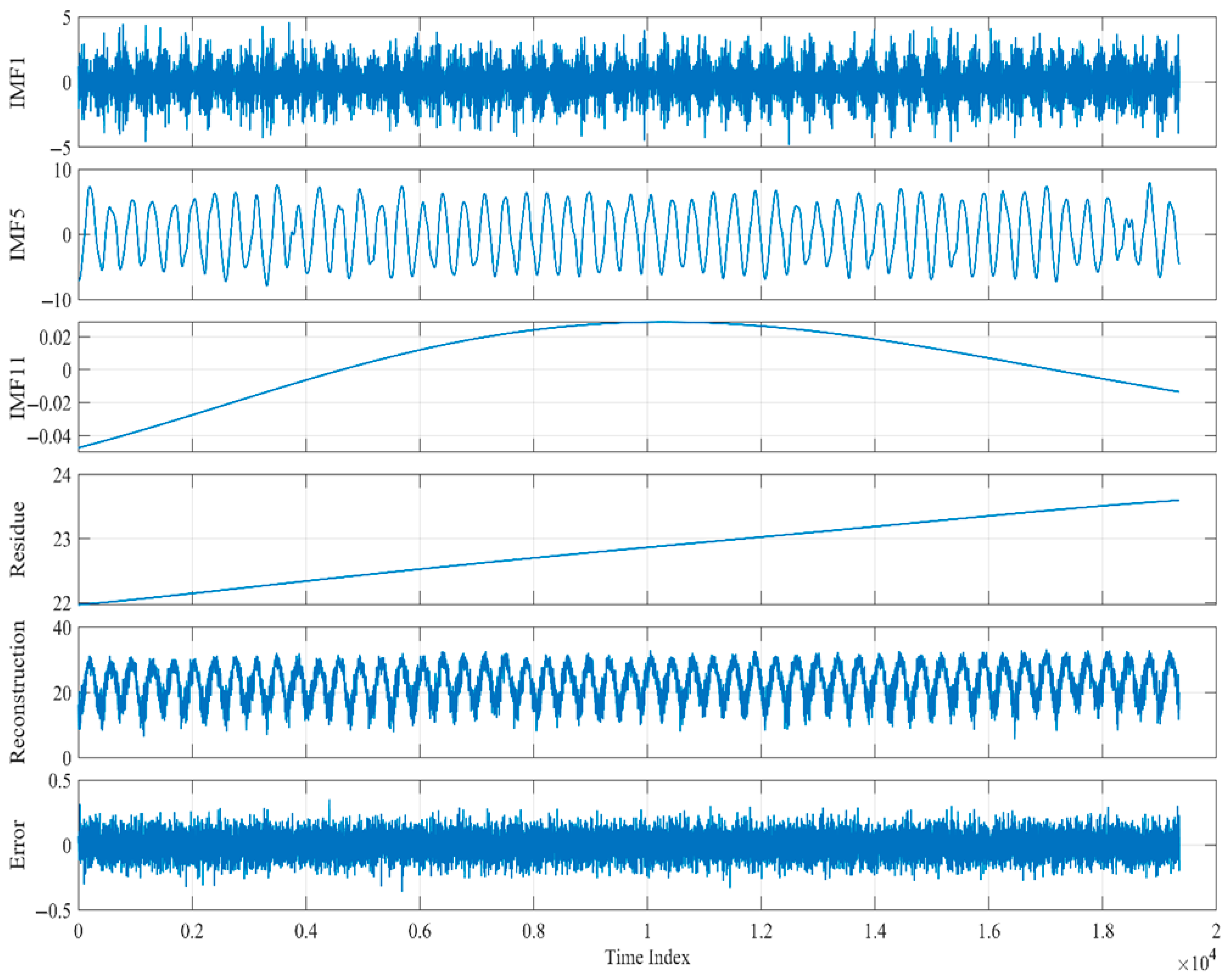
After applying EMD to the Taipei Observatory’s daily temperatures from 1971 to 2023, the residual trend, reconstructed series, and original data are presented together in Figure 10. These subplots reveal that IMF1–IMF4 capture high-frequency, small-amplitude fluctuations on daily to monthly scales; IMF5 exhibits a regular seasonal oscillation whose peaks and troughs align closely with spring, summer, autumn, and winter temperature cycles; IMFs 6–10 sequentially represent low-frequency variations spanning multiple years to over a decade; and IMFs 11–12 have negligible amplitudes, effectively constituting ultra–low-frequency remnants or numerical noise. The residual trend rises gently from about 22.0 °C to 24.0 °C, reflecting the overall warming trend. Figure 10 highlights representative components: IMF1, IMF5, IMF11, the residual, and the reconstruction error, to illustrate oscillations and trends at different time scales, demonstrating EMD’s effectiveness at separating daily volatility, annual cycles, and long-term change. When all IMFs and the residual are recombined, the “Sum” series virtually overlaps the original data: the mean reconstruction error is −1.8309 × 10⁻⁴ °C with a standard deviation of 2.7376 × 10⁻² °C, confirming the high accuracy of the decomposition and reconstruction.

To quantify the characteristic period of each IMF, this study employed a zero-crossing analysis: by tracking each transition of the IMF from positive to negative (or vice versa) across the zero axis, the duration of each oscillation is identified, and the average of all these oscillation lengths is taken as the representative period of that IMF [25]. Additionally, the energy of each IMF is computed as $E\mathrm{i}={\sum }_{\mathrm{t}}{\left|A_{\mathrm{i}}\right(t\left)\right|}^2$, and its relative weight is given by $W_{\mathrm{i}}=E_{\mathrm{i}}/{\sum }_{\mathrm{j}}{E}_{\mathrm{j}}$. According to the results in

Table 1. IMF periods and weight ratios from daily data decomposition.

	Period (Days)	Energy Weight (%)
IMF1	3.37	4.87
IMF2	8.15	5.75
IMF3	18.9	3.66
IMF4	45.8	1.8
IMF5	352.9	78.18
IMF6	376	5.23
IMF7	1251	0.29
IMF8	3486.8	0.18
IMF9	5290.67	0.05
IMF10	11307	1.12 × 10−3
IMF11	N/A	3.22 × 10−3

, the fifth IMF has an average period of approximately 360 days, while the mid- to high-order IMFs span hundreds to thousands of days; IMFs 11–13 exhibit very long periods but possess near-zero amplitude and weight. Table 1 shows that IMF5’s energy weight reaches 0.78, far exceeding that of any other component, underscoring its dominant role in the temperature series; by contrast, IMFs 12 negligibly to reconstruction and may be effectively ignored.

Overall, because IMF5 combines the highest energy weight with a period corresponding precisely to the annual cycle, this study uses a one-year base for IMF decomposition when segmenting and synthesizing each year’s data. This choice ensures that seasonal oscillations at the annual scale are fully preserved and provides a stable, reliable periodic framework for the synthesis and forecasting models.

3.3. Urban Temperature Simulation Framework Based on a Process Moving Process

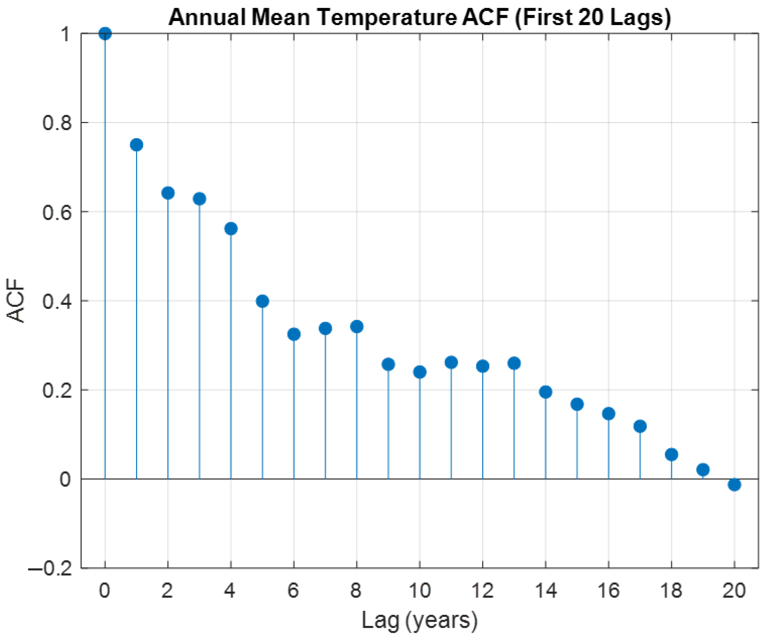
This study divides the daily temperature record from the Taipei Observatory (1971–2023) into 53 annual segments and applies Ensemble Empirical Mode Decomposition (EEMD) to each, extracting seven IMFs plus a residual to capture multi-scale oscillations and long-term trends. To determine an appropriate 5-year moving process length, we performed an autocorrelation analysis on the 53 annual mean temperatures (Figure 11). With 53 samples, the 95% white-noise confidence bound is approximately ±0.27. The lag−5 autocorrelation remains slightly above this threshold, whereas lags of six years and beyond fall well within the confidence interval, indicating strong linear persistence up to five years but not beyond. Accordingly, we selected a process to preserve interannual memory while avoiding excessive statistical noise and computational complexity.

The simulation workflow is illustrated in Figure 12: first, we reconstruct and project daily temperatures for 1976 using the IMFs and residual from 1971 to 1975; then we slide the process forward, using 1972–1976 to project 1977, and so on through 2023. With L = 5 and p = 7, the total number of possible synthetic annual sequences is 5⁸ = 390,625; by contrast, L = 4 yields only 4⁸ = 65,536 combinations. Considering both the need for a diverse ensemble and computational feasibility, we adopted L = 5 as the optimal base length, balancing richness of simulation space with manageable computational load.

For validation, we compared the simulated versus observed annual mean temperatures from years six through fifty-three (Figure 13). In normal years such as 1981, 1982, 1999, and 2000, the simulated median curve (in red) closely overlaps the observed interquartile ranges each month, successfully reproducing the transition from winter lows to summer highs. In contrast, extreme years: 1997, 2014, 2015, and 202 show that simulations generally underpredict observed peaks and troughs; under severe heatwave or cold-spell events, the process-process method’s reliance on smoothed historical averages cannot fully capture sudden anomalies, causing simulated curves to deviate noticeably from the observed boxplots.

Overall, the strategy of decomposing IMFs on an annual basis with a 5-year moving process yields strong performance in reproducing Taipei’s urban temperature cycle and provides a practical framework for generating over a million synthetic samples; however, because its predictions rely heavily on the process historical average, its ability to anticipate extreme deviations remains limited. Future work could integrate climate anomaly indices or introduce nonlinear coupling factors to enhance simulation and forecasting accuracy for extreme-year sequences.

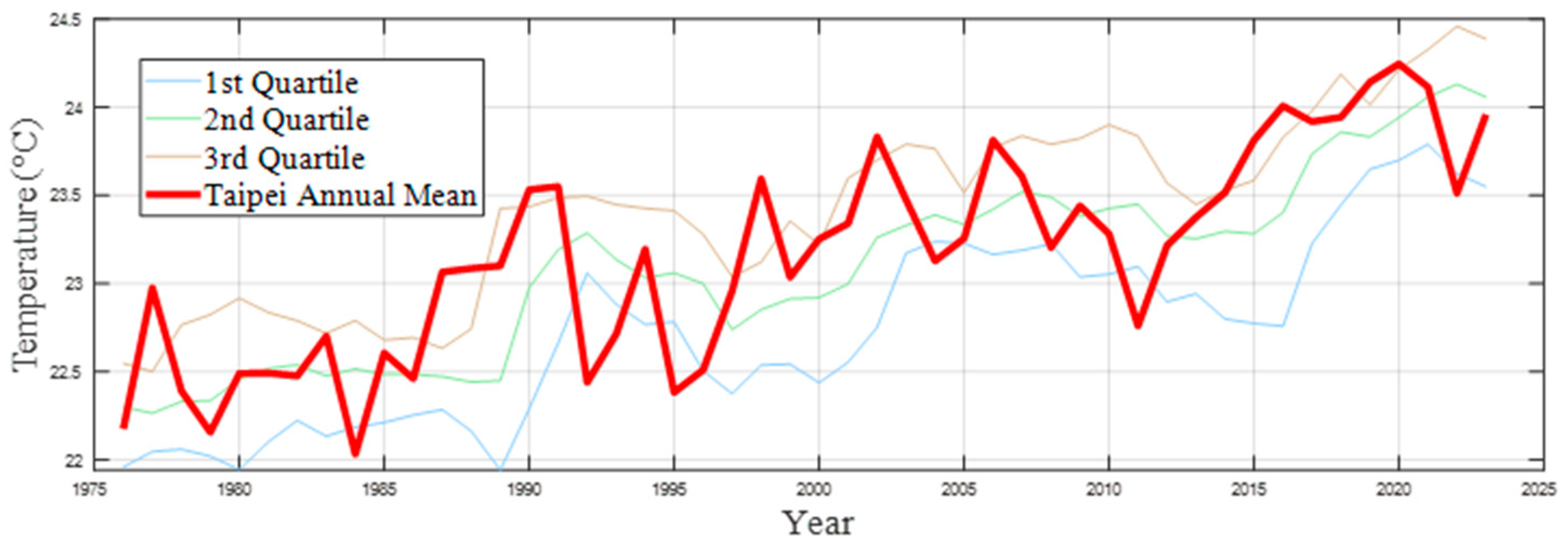
Figure 14 shows annual projection from 1971 to 2023 that uses a 5-year moving process together with EMD. Except for a few extreme years, such as 1981, 1997, and 2015, most actual annual means fall within the first to third quartile ranges of the simulated boxplots, and the marked outliers closely match the recorded maximum and minimum values. This indicates that the simulations, reconstructed from IMFs and residuals of the preceding five years, effectively reproduce Taipei’s annual temperature fluctuations and capture the multi-scale variability inherent in nonstationary sequences. However, during extreme heat or cold events, the smoothing effect of the 5-year moving process causes the simulated curves to lag in reflecting sudden anomalies, resulting in lower prediction accuracy in those years. Overall, the 5-year moving process demonstrates excellent performance in replicating normal-year temperature patterns and offers a robust, representative tool for statistical simulation of long-term urban temperature trends.

3.4. Monthly Temperature Level Forecast

After completing the IMF decomposition based on the 5-year moving process and simulating daily temperatures, this study classified the resulting synthetic series into five categories: Cold, Cool, Moderate, Warm, and Hot, and then calculated the proportion of days in each category for every month. Specifically, for each simulated year, we computed the percentage of days in each month that fell into each level based on 390,625 synthetic daily mean temperature records, thereby estimating the monthly category distribution. Figure 15 illustrates these monthly distributions across the five temperature levels for representative years 1981, 1982, 1997, 1999, 2000, 2014, 2015, and 2023, clearly revealing how the structure of temperature categories varies with seasonal transitions and extreme events. In typical years such as 1981 and 1982, January–February is dominated by the “Cool” category, March–May falls almost entirely within “Moderate,” June–August sees “Warm” exceed 90%, September–October alternates between “Moderate” and “Warm,” and November–December returns to predominantly “Moderate”. Years 1999 and 2000 exhibit similar seasonal transitions, faithfully reflecting the progression from winter through peak summer and back to autumn-winter. Notably, during late spring (April–May) and early autumn (October–November), temperatures remain largely within the “Moderate” range (18–27 °C), demonstrating stability in classification during these transitional periods.

By contrast, in heat-biased years such as 1997 and 2015, the “Warm” category approaches 100% in June–September, with “Hot” (>32 °C) days already appearing in July and August. In 2014 and 2023, intensified urban heat island effects lead to significant shares of both “Moderate” and “Warm” categories throughout the year. The “Cold” category appears only briefly in specific extreme-cold early and deep winter seasons, and the frequency of “Cool” days has declined markedly.

The projected annual temperature series are based on the 390,625 synthetic samples. The accuracies can be cross-validated using a combination of box plots and level classification. The results show that, in recent decades, Taipei’s daily mean temperatures have become heavily concentrated in the “Moderate” and “Warm” intervals. While “Cold” and “Hot” extremes remain relatively rare, their occurrence frequency has trended upward, highlighting the importance of tail-end climate variability.

Classification accuracy is, however, limited by static threshold boundaries. Comparing simulated versus observed monthly distributions from 1981 to 2023 yields overall accuracy between 60% and 71%, with an average of approximately 65.1%. In extreme heat years (e.g., 2015, 1997), multiple days exceeding 32 °C are often misclassified as “Warm” or even “Moderate,” reducing accuracy. Similarly, in extreme cold years such as 1981, the simulated frequency of “Cold” days is significantly underestimated, failing to capture cold-pulse events.

4. Conclusions

This study used daily temperature records from the Taipei Observatory (1971–2023) as a case study. The purpose is to develop and validate a non-stationary sequence projection based on Empirical Mode Decomposition (EMD). The results show that Taipei’s annual mean temperature has risen steadily at approximately 0.02 °C per year, resulting in a total increase exceeding 2 °C, with summer daily maxima increasing significantly and winter daily minima declining, reflecting the combined impact of urban warming and the heat island effect. The multi-scale oscillatory components extracted by EMD not only reproduce temperature fluctuations from daily to annual scales but also capture long-term trends through the residual term, providing a robust tool for analyzing non-stationary climate series.

In data projection and classification, synthetic daily temperatures based on a 5-year process were categorized into five levels (Cold, Cool, Moderate, Warm, and Hot), and their monthly probability distributions were compared against observations. Overall classification accuracy ranged from 60% to 71%, with an average of 65.1%, demonstrating the method’s reliable consistency in reproducing seasonal and annual cycles.

In practical terms, the EMD-based decomposition framework presents significant utility in early detection of temperature anomalies and seasonal extremes. One key strength lies in its ability to pre-classify synthetic temperature series into distinct categories, enabling seasonal forecasts of high-temperature frequencies. Such pre-classification can be directly translated into year-scale early warning systems. By using historical temperature distributions and projecting short-term category probabilities, urban administrators can anticipate warm-to-hot periods with higher lead time than conventional stationarity-based statistical methods [5,6].

This framework also allows adaptive refinement of classification thresholds. The current five-level temperature classification can be dynamically adjusted using percentile-based or quantile-normalized benchmarks, improving accuracy under changing climate baselines [18]. A more granular categorization (such as expanding to seven or nine classes) could improve detection of extreme high-temperature clusters, which are particularly relevant for health risk advisories, school safety measures, and infrastructure stress testing [4,5]. By continuously recalibrating the synthetic temperature distributions using rolling observations, the model can sustain relevance under continued warming, as suggested in dynamic recalibration practices seen in seasonal forecasting systems [6].

Beyond temperature prediction alone, this study’s findings have promising applications in urban hydrological risk management. Temperature changes influence urban water cycles through multiple feedback pathways. Warmer air enhances evapotranspiration, reduces soil moisture, and increases runoff peaks when combined with intense rainfall. Using projected temperature categories, municipalities can preemptively assess water demand surges and potential soil drying prior to peak summer [7]. Urban runoff models such as SWMM or MIKE URBAN, when integrated with high-temperature forecast classes, can simulate compound risk scenarios involving both heat and flash flooding, particularly when temperature-induced convective precipitation events are common.

Moreover, longer heat periods may lead to reduced infiltration and increased pollution accumulation on impervious surfaces, which can be flushed during storm events, degrading urban water quality. Proactive temperature-based early warning systems can help trigger pre-rainfall cleanup operations or stormwater diversion protocols. In this context, the EMD-based forecast sequence offers city planners an anticipatory tool that integrates climate signals into infrastructure readiness strategies.

Health-related sectors may also benefit. High-temperature classes derived from this system could be used to estimate heat risk indices, such as the Wet Bulb Globe Temperature (WBGT), particularly when coupled with humidity forecasts. Elderly populations and outdoor workers could receive tailored alerts based on projected category frequencies, not just raw temperatures. Additionally, heat-energy models used in power grid operation can incorporate probabilistic outputs from the EMD system to anticipate cooling demand spikes, as has been proposed in urban energy–climate interaction studies [11].

Despite these strengths, several limitations should be acknowledged. First, the classification accuracy is sensitive to how temperature thresholds are defined. When climate baselines shift, static thresholds may no longer reflect the same physical or statistical meanings, leading to biased comparisons [22]. Second, the EMD method is vulnerable to the influence of extreme events. Strong outliers, such as record-breaking heatwaves, may distort mode separation and lead to artificial trends in the decomposition [24]. Finally, the method requires long, continuous, and homogenized data series. Gaps or discontinuities in meteorological records may impair the accuracy of mode extraction, especially for low-frequency components.

In conclusion, this paper demonstrates the effectiveness and superiority of Empirical Mode Decomposition (EMD) in projecting non-stationary air temperatures observed at meteorological stations. The conclusion is consistent with previous findings on sea surface temperature projections, reinforcing EMD’s generalizability across domains. The five-year moving window decomposition and reconstruction process generates realistic temperature ensembles with structured variability, enabling robust simulation of category distributions and long-term trends. Looking forward, the method’s potential lies not only in reproducing climatic behavior but also in delivering early warning capacity, adaptive threshold tuning, and cross-sectoral integration, particularly in urban hydrological planning and extreme climate risk mitigation.