Abstract
Tai Lake Basin, a key freshwater resource in eastern China, has garnered attention due to widespread cyanobacterial blooms. Effective water quality management is vital for the region’s sustainable development. Investigating the seasonal variations of water quality parameters (WQPs) in Tai Lake Basin is essential for devising targeted strategies to enhance water quality. This study employs an interpretable machine learning model (XGBoost-SHAP) to identify the most important factors of water quality using daily monitoring WQP data from 2023 to 2024. Results revealed that dissolved oxygen (DO), total phosphorus (TP), permanganate index (CODMn), and ammonia nitrogen (NH3-N) are primary determinants of water quality in the basin, while water temperature, pH, total nitrogen (TN), and turbidity showed minimal impact (SHAP value < 1). Seasonal analysis demonstrated that DO exerts a substantial influence on water quality during spring, summer, and autumn; TP and CODMn have a stable and negative impact on water quality throughout the year; NH3-N has a relatively significant negative impact on winter water quality. Recommendations include enhancing DO levels in spring and summer, fortifying TP and NH3-N concentrations in winter, and implementing tailored strategies in response to seasonal variations. This research offers valuable insights to guide decision-making processes aimed at enhancing water quality and safeguarding the water environment in the Tai Lake Basin.
1. Introduction
Water quality encompasses the chemical, physical, biological, and radioactive attributes of water that dictate its suitability for various purposes, including drinking, recreational activities, and supporting aquatic life. It plays a pivotal role in shaping the management and exploitation of water resources and the overall health of aquatic ecosystems [1]. The escalating global water scarcity and pollution underscore the critical importance of water quality assurance for human health and ecosystems. The United Nations Sustainable Development Goals mandate the universal guarantee of clean drinking water. Consequently, identifying the pivotal factors influencing water quality is paramount for devising evidence-based water quality management policies and advancing the sustainable exploitation of water reserves.
The analysis of key influencing factors of water quality mainly includes two methods: mechanistic analysis methods and non-mechanistic analysis methods [2,3]. Mechanistic analysis methods rely on the dynamics of physical processes within water bodies, focusing on constructing models of physical, chemical, and biological processes to elucidate causal relationships in water quality changes. These methods are advantageous due to their parameters’ strict physical interpretations, enabling realistic simulations of various transport and transformation processes from a systematic perspective. Nonetheless, challenges such as challenging parameter calibration, complex modeling structures, uncertain model parameters, and high computational costs restrict their use in predicting watershed water quality [4]. The mechanistic analysis method originated from the Streeter–Phelps model proposed in 1925 by American scholars H.W. Streeter and E.B. Phelps after their kinetic research and analysis of the oxygen consumption process. This model is capable of replicating the patterns of variation in biochemical oxygen demand (BOD) and dissolved oxygen (DO) levels in river systems [5]. Following the launch of the QUAL-I water quality comprehensive model by the US National Environmental Protection Agency in 1970, subsequent iterations, including QUAL-II, QUAL 2E, QUAL 2E-UNCAS, and QUAL2K, were developed to model the migration and transformation of both common and toxic pollutants in diverse water bodies. These versions are extensively applied in water quality forecasting, as well as in the design and management of river water treatment systems [6,7]. Similarly, the SWAT model was developed by the Agricultural Research Center of the United States Department of Agriculture in 1994 to replicate surface water and groundwater quality dynamics in watersheds primarily characterized by agriculture and forests [8]. The SWAT model has found extensive application in the simulation of non-point source pollution.
Non-mechanistic water quality analysis methods offer a promising alternative to traditional mechanistic analysis methods. These data-driven techniques can effectively model complex nonlinear relationships within large datasets, circumventing the need for detailed system modeling and explicit causal formulations. By solely relying on historical water quality records, predictive models can be established without requiring prior knowledge of the underlying physical processes and parameters [9]. This approach has seen widespread practical application and holds the potential to complement or even supplant mechanistic models in future water quality forecasting endeavors [10,11]. Common analytical techniques for non-mechanistic factors encompass regression analysis, time series analysis, grey system analysis, and neural network analysis [12]. In recent years, the application of non-mechanistic water quality analysis methods in water quality prediction and influencing factor analysis has gradually become a research hotspot [13]. Rajaee et al. [14] conducted a comprehensive evaluation of diverse water quality simulation models, revealing a notable enhancement in prediction accuracy upon the incorporation of neural networks. Noori et al. [15] introduced a novel full convolutional neural network (FCNN) architecture that integrates SWAT models to achieve precise water quality predictions. Similarly, Samsudin et al. [16] employed artificial neural networks (ANNs) to forecast the seawater quality index in the mangrove Estuary region, demonstrating superior predictive performance compared to the traditional multiple linear regression approach. Ta et al. [17] utilized convolutional neural networks (CNNs) to forecast dissolved oxygen (DO) levels, demonstrating superior predictive accuracy compared to conventional BP neural networks. To enhance the interpretability of machine learning models, Lundber [18] introduced the SHAP framework in 2017, validating its efficacy through empirical studies. Lubo-Robles [19] employed SHAP interpretation on random forest classifiers to assess the significance of seismic attributes and methodologies in machine learning model predictions. Batunacun et al. [20] examined 20 drivers through XGBoost analysis and employed SHAP values based on data from the Silingrad steppe to elucidate the outcomes of a purely data-driven approach. Their findings underscored the utility of SHAP values in assessing intricate interrelationships among various drivers of grassland degradation. In a similar vein, Morita et al. [21] demonstrated the capacity of machine learning models to capture physical phenomena effectively through SHAP interpretation analysis, thereby enhancing predictive accuracy.
The use of XGBoost in combination with SHAP has become common in water quality studies, particularly for identifying key influences. Niazkar et al. [22] reviewed the use of XGBoost in water resources engineering and water quality studies from December 2018 to May 2023 and found that in 74% of the papers, XGBoost or its hybrid models outperformed other machine learning models in a variety of applications. Merabet et al. [23] used six machine learning models, including XGBoost, for predicting dissolved oxygen (DO) concentration, water turbidity, and chlorophyll-a levels in the Illinois River, USA. SHAP was used for model interpretability and feature ranking, and it was shown that SHAP improved the understanding of the contribution of each variable in the final predictions. Kruk [24] utilized the XGBoost-SHAP model to analyze factors affecting cyanobacteria concentration in the Vistula Lagoon, Baltic Sea. Park et al. [25] developed an XGBoost-based machine learning model with 18 input variables to predict chlorophyll a (Chl-a) concentration. Their findings indicated that the model achieved optimal stability when SHAP determined the input variable priorities.
The water quality of Tai Lake has been the subject of extensive scholarly investigation [26]. Since the turn of the century, the lake has garnered international attention due to the prolific growth of cyanobacteria [27]. Research on the water quality of Lake Tai has broadly progressed through three phases. The initial stage, spanning the late 20th to early 21st century, focused on establishing a foundational understanding of the water quality issues. Scholars primarily concentrated on characterizing the basic conditions and pollution profiles of the lake. The subsequent phase in the early 21st century saw the exploration of water quality assessment methodologies to more precisely evaluate the state of the lake. Most recently, the rapid advancement of monitoring technologies, data science, mathematical modeling, and machine learning has enabled the study of influential factors and predictive modeling of water quality in the Lake Tai Basin, yielding high-accuracy forecasts. Tan et al. [28] developed a data-driven model leveraging quadratic modal decomposition and multidimensional external features to predict dissolved oxygen (DO) levels in Tai Lake. This model excelled in prediction accuracy and effectiveness, establishing a mechanism for water temperature regulation that supports water resource protection and fishery management. Xu et al. [29] created a three-dimensional water environment model for Tai Lake, integrating it with uncertainty and sensitivity analyses to identify key factors controlling total phosphorus (TP), total nitrogen (TN), dissolved oxygen (DO), and chlorophyll a (Chl-a), thereby providing vital insights for eutrophication management. Zhou et al. [30] introduced a water quality prediction method using an improved grey relational analysis (IGRA) algorithm combined with a long short-term memory (LSTM) neural network, specifically applied to Tai Lake’s water quality. Sun et al. [31] employed a machine learning model to forecast chlorophyll a (Chl-a) concentrations in Tai Lake. Ananias et al. [32] developed an algal bloom forecasting (ABF) framework utilizing MODIS time series and climate data, integrating support vector machine (SVM), random forest (RF), and long short-term memory network (LSTM) techniques for anomaly detection. Their findings indicate that machine learning models markedly enhance the accuracy of algal bloom predictions. While numerous studies have examined the spatial differentiation of water quality in Tai Lake, few have explored the seasonal variation laws of influencing factors. Despite the variety of prediction methods, some fail to systematically explain the influencing factors of water quality in the Tai Lake Basin.
This study focuses on the Tai Lake Basin, employing the XGBoost-SHAP method to systematically analyze the factors affecting water quality [33]. It uncovers the distinct characteristics of key influences, providing a precise basis for water quality management decisions in the region. The innovation of this paper lies in the fact that, considering the significant seasonal differences in water quality in the Tai Lake Basin, a comprehensive analysis of the factors influencing water quality in the Tai Lake Basin is conducted based on daily monitoring data. The data are further split by season to analyze the key influencing factors and their dependency relationships in each season. Compared with existing studies, this research can not only identify the key influencing factors of water quality throughout the year but also reveal the specific influencing patterns in different seasons, which is conducive to achieving refined management of water resources in the Tai Lake Basin and makes up for the deficiencies of existing studies.
2. Materials and Methods
2.1. Method
Extreme Gradient Boosting (XGBoost) is a highly efficient, versatile, and portable gradient boosting framework known for its exceptional performance optimization, automatic treatment of missing values, compatibility with various objective functions and custom loss functions, and a wide range of parameter tuning capabilities to streamline model refinement [21]. In conjunction, SHAP offers visual insights into model inputs and outputs. Consequently, the integration of XGBoost and SHAP models is employed to assess the determinants of water quality.
2.1.1. XGBoost
XGBoost is an optimized gradient boosting framework that offers a flexible, efficient, and portable solution [34]. Developed by Chen and Guestrin [35], it builds on the Gradient Boosting Decision Tree (GBDT) and employs various strategies to enhance performance and computational efficiency. XGBoost is based on the concept of utilizing decision trees as fundamental learning units to construct a high-performing predictive model through iterative training and aggregation of multiple models. It employs a gradient boosting approach to sequentially introduce new weak learners in each iteration, leveraging the outcomes of the preceding iteration to rectify errors in the training dataset. In contrast to conventional decision trees, XGBoost effectively manages model complexity and mitigates overfitting risks by incorporating regularization terms and a feature selection mechanism [36].
Within the XGBoost model, the feature selection process is pivotal for recognizing and leveraging essential features. Its fundamental objective is to assess the significance of each feature and ascertain which ones predominantly enhance model performance. This mechanism in XGBoost comprises three key elements: assessing feature importance, eliminating less impactful features, and incorporating features that notably enhance model performance.
In the training phase of XGBoost, feature selection is conducted using a tree-based strategy to assess the significance of each feature. As trees are built, the model monitors and logs the impact of each feature during node splits, subsequently aggregating these impacts to determine feature importance [37]. After determining the significance of features, the model can exclude less important features using predefined thresholds or alternative strategies. This process offers the benefit of reducing model dimensionality, filtering out noise and irrelevant data, thereby enhancing model efficiency. The XGBoost algorithm comprises five distinct steps [38,39].
Step 1: Initialization. During XGBoost training, a weak learner, typically a basic decision tree, is first initialized. The predictions from this initial model serve as the starting point for subsequent iterations, known as the initial estimate. In regression tasks, the initial model’s constant value is often the mean of the target variable, while in classification tasks, it may represent an initial class probability distribution. In regression, the model predicts values, whereas in classification, it predicts probability values for each category. The variance lies mainly in the choice of loss function, with the fundamental principle remaining consistent across both scenarios.
Step 2: involves computing the gradient. In XGBoost training for regression tasks employing Mean Squared Error (MSE) as the loss function, the model computes the gradient for each individual sample. This gradient signifies the disparity between the actual value and the present model prediction, thereby indicating the prediction error of the model for the given sample at its current state:
where and are true and predicted values, respectively. The partial derivative of the loss function to is:
This is the partial derivative of the loss function with respect to the predicted value. For the log-likelihood loss function of the classification problem, the gradient is calculated as follows:
where is the true category (0 or 1), and is the probability that the model predicts a category of 1. The partial derivative of the loss function on is:
This is the partial derivative of the loss function for the probability of predicting class 1.
Step 3: Decision trees are fitted. During the training process of XGBoost, a new decision tree is incorporated to enhance the accuracy of the existing model by capturing residual errors. In regression tasks, the decision tree is built by minimizing the sum of squared gradients, while for classification tasks, optimization is achieved through the negative gradient of the log-likelihood loss function. XGBoost employs and regularization techniques during the construction of the decision tree to manage model complexity effectively and mitigate the potential for overfitting.
The objective function of the XGBoost model is:
Step 4: involves updating the model in XGBoost training. Upon constructing a new decision tree, it is incorporated into the existing model to minimize errors from the previous iteration. To maintain model stability, XGBoost incorporates a hyperparameter known as the learning rate, which regulates the influence of each new tree on the overall model. Fine-tuning the learning rate allows for a trade-off between training speed and prediction accuracy, thereby ensuring model stability throughout the iterative process.
Step 5: Iteration. Steps 2 to 4 are reiterated until a specified number of iterations or a termination condition is met.
The ultimate model comprises a weighted aggregation of decision trees generated across multiple iterations, with each tree’s influence finely adjusted by the learning rate and regularization term. This meticulously crafted model is subsequently applied in predictive and classificatory tasks. XGBoost employs a gradient boosting algorithm to sequentially enhance the loss function and adeptly incorporate regularization terms for constructing a sequence of effective decision tree models. This iterative process not only enhances model performance significantly but also ensures robust generalization capabilities when confronted with novel data.
The commonly used indicators for model evaluation include precision, accuracy, recall, and , with the formula as follows:
In the context of predictive modeling, the following symbols are commonly used: for correct predictions, for prediction errors, for the sample, for the negative sample, for true positives (positive samples correctly predicted as positive), for false positives (negative samples incorrectly predicted as positive), for false negatives (positive samples incorrectly predicted as negative), and for true negatives (negative samples correctly predicted as negative).
2.1.2. SHAP
The Shapley Additive Explanations (SHAP) method is employed for interpreting model outputs by attributing contributions to each input feature [40]. The SHAP value of each feature determines its impact and direction on the prediction results. By integrating physical laws and empirical knowledge, the reliability of model predictions can be assessed based on SHAP values [41].
A positive SHAP value indicates a positive impact of the feature on the model’s prediction, while a negative value signifies a negative impact. The SHAP method is valuable for ranking feature importance, with the magnitude of the SHAP value directly correlating with a feature’s significance in the model. The predicted value for a specific sample is determined by adding the SHAP value for that sample to the model’s baseline value, typically set as the average of all sample target variables.
Let the -th sample be denoted as , where the -th trait of the ith sample is represented as . The prediction value of the model for this sample is denoted as , while the reference value of the entire model (typically the mean of all sample target variables) is denoted as . Let represent the SHAP value of the -th feature of the -th sample. In this context, the SHAP value adheres to the subsequent formula [42]:
where is calculated as follows:
Let represent the comprehensive set of influencing factors for sample , and let denote an arbitrary subset of influencing factors within sample . The term signifies the combined impact of the influencing factors within subset , while quantifies the contribution of factor to the collective effect. The SHAP value for influencing factor is computed by aggregating and averaging the contributions of factor across all samples, according to the following formula:
2.1.3. XGBoost-SHAP Model
The XGBoost model and SHAP interpretation framework algorithm were utilized to analyze surface water quality data from the Tai Lake Basin. The collected data underwent preprocessing to ensure quality and suitability for model training. Finally, three-fold cross-validation was used to train and evaluate the model [43].
The XGBoost algorithm is utilized during the model training phase. Following training, the model undergoes evaluation using the test set, primarily focusing on its accuracy indicator. In cases where the accuracy falls short of expectations, adjustments are made to the model parameters, and its performance is improved through iterative optimization.
Ultimately, the machine learning model achieving optimal performance is acquired. By employing SHAP for interpretative analysis of water quality influencers, pivotal factors impacting water quality are unveiled. The workflow of the XGBoost-SHAP model is depicted in Figure 1 [44].
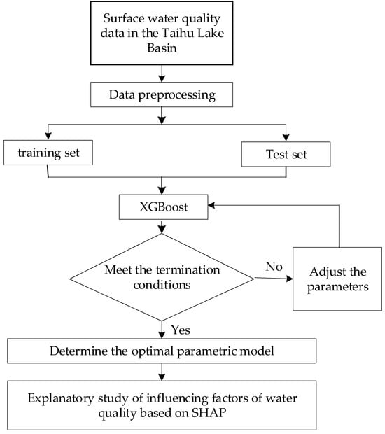
Figure 1.
Flowchart of the analysis of key influencing factors of water quality based on the XGBoost-SHAP model.
2.2. Data Source and Preprocessing
2.2.1. Study Area
The Tai Lake Basin, situated in the lower Yangtze River Delta in China, spans three provinces—Jiangsu, Zhejiang, and Anhui—and the municipality of Shanghai. Renowned for its economic development, the basin encompasses numerous lakes and includes all of Suzhou, Wuxi, and Changzhou in Jiangsu, parts of Zhenjiang and Nanjing, all of Jiaxing and Huzhou in Zhejiang, part of Hangzhou, the mainland of Shanghai (excluding Chongming, Changxing, and Hengsha Islands), and sections of Xuancheng in Anhui. Covering 36,900 km2, the basin is distributed as follows: Jiangsu (52.6%), Zhejiang (32.8%), Shanghai (14.0%), and Anhui (0.6%). The basin’s water environment is crucial for residents’ safety, ecological balance, and regional sustainable development, underpinning the area’s socio-economic sustainability.
In recent years, accelerated urbanization and intensified human activities have posed unprecedented challenges to the Tai Lake Basin’s water environment. The aquatic ecosystem is under severe strain, with frequent eutrophication and cyanobacterial blooms emerging as significant barriers to regional sustainable development [45,46]. Thus, enhancing water quality management in the Tai Lake Basin is imperative for maintaining ecological health and sustainability [47]. Identifying and analyzing the key factors influencing water quality is crucial in this effort.
2.2.2. Data Description and Preparation
Data for this study were obtained from the National Real-time Surface Water Quality Automatic Monitoring Data Release System of the China National Environmental Monitoring Centre. Hourly data from March 2023 to February 2024 for the Tai Lake Basin were collected, covering nine key indicators: water temperature, pH, dissolved oxygen (DO), permanganate index (CODMn), ammonia nitrogen (NH3-N), total phosphorus (TP), total nitrogen (TN), electrical conductivity, and turbidity. The initial water quality data undergo preprocessing through data cleaning to ensure their reliability and validity, thereby enhancing the accuracy of subsequent analyses [48]. Given the pros and cons of various techniques for handling missing values and the specific characteristics of water quality data, the median imputation method is chosen for indices with few missing entries. Outlier detection is employed to identify potential issues, optimize data quality, and improve the precision of subsequent analyses and conclusions.
Post-cleaning, 165,561 data points were available. Descriptive statistics of these data are presented in Table 1.

Table 1.
Descriptive statistics of the data.
Table 1 reveals a mean water temperature of approximately 20 °C, with a standard deviation of 8.17 °C, indicating significant variability from 1.4 °C to 36.3 °C. The pH of the water sample exhibited remarkable stability, fluctuating minimally around a mean value of 7.66 with a standard deviation of only 0.36. This narrow range indicates that the water maintained a consistently neutral to slightly alkaline state throughout the observation period.
The mean DO content is 7.24 mg/L, suggesting a moderate level in the water, with a standard deviation of 2.48 indicating variability. The CODMn averages 3.24 mg/L, reflecting the typical concentration of organic pollutants. Additionally, ammonia nitrogen, TP, and TN display their own fluctuation patterns.
The mean conductivity was 469.73 μS/cm with a standard deviation of 127.41, highlighting notable variability in ion concentration. The average turbidity measured 47.96 NTU, with a standard deviation of 28.80, indicating significant spatial differences, from nearly clear water at 0.005 NTU to highly turbid water at 145.16 NTU.
3. Results and Discussion
3.1. Model Parameter Selection and Accuracy Evaluation
This study employs XGBoost-SHAP to identify the primary factors affecting water quality. The XGBoost model incorporates parameters like the maximum number of iterations, learning rate, and decision tree depth (Table 2). To enhance result accuracy, grid search and cross-validation are utilized to determine the optimal hyperparameter combination.
Table 2.
Parameter tuning settings and meanings of XGBoost.
The model’s performance was assessed using precision, accuracy, recall, and , as detailed in Table 3.
Table 3.
Model evaluation results.
The overall accuracy, along with seasonal accuracies, were 96.4%, 97.3%, 96.9%, 98.1%, and 97.1%, respectively. The consistent recognition accuracies across the five datasets suggest the model does not suffer from overfitting. Additionally, recall, precision, and scores were notably high, demonstrating the model’s strong recognition capabilities.
3.2. Analysis of Influencing Factors on Water Quality
This study utilizes the SHAP framework to explore the relationship between nine dataset features and water quality, focusing on factor contributions and dependence graphs. Figure 2 displays the SHAP values for all influencing factors, with each point representing a prediction sample. The X-axis denotes the SHAP value (factor influence on output), while the Y-axis lists the influencing factors, ordered by importance from top to bottom.
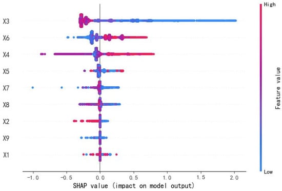
Figure 2.
SHAP values of the impact factor for the overall data.
Figure 2 illustrates the influence of various factors on the model output through color coding: blue indicates a positive influence, with deeper shades signifying stronger positive effects on water quality, while red denotes a negative influence, with deeper shades indicating stronger negative effects. For a given factor, a larger blue proportion suggests a stronger positive influence compared to the negative, and vice versa. The extent of the SHAP value range for a factor reflects the significance of its impact on water quality.
Figure 2 reveals that the SHAP value for DO (X3) spans the widest range, underscoring its predominant influence on water quality. An increase in DO (X3) positively affects water quality. Conversely, TP (X6) and the CODMn (X4) significantly negatively impact water quality as their levels rise. NH3-N (X5), TN (X7), and electrical conductivity (X8) also affect water quality to some extent. Water temperature (X1), turbidity (X9), and pH (X2) exhibit SHAP values fluctuating around zero, indicating a minor impact on water quality, as evidenced by their narrow range and balanced red–blue proportions. Notably, increases in TP (X6), permanganate (X4), NH3-N (X5), and TN (X7) may contribute to water quality degradation [29].
3.3. Analysis of Influencing Factors on Seasonal Water Quality
Fang, L. et al.’s analysis of Huzhou’s Tai Lake surface drinking water from 2011 to 2015 identifies excessive TN and TP as primary concerns, potentially fostering algal blooms. Key indicators surpassing national standards include TN, iron, and manganese. Seasonal fluctuations are evident in chemical oxygen demand, DO, NH3-N, and TN [49]. This study further examines the SHAP values of influencing factors across four seasons to elucidate seasonal similarities and differences, as depicted in Figure 3.
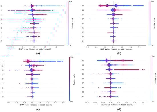
Figure 3.
SHAP values influencing factors across seasons: (a) spring, (b) summer, (c) autumn, and (d) winter.
Figure 3 illustrates that each season may have dominant parameters that significantly affect the model output. DO (X3) positively influences water quality in spring, summer, and autumn but has minimal impact in winter. Thus, increasing DO in these seasons enhances water quality. Water temperature, algal growth, and human activities primarily drive the seasonal variation of DO. In summer, high temperatures cause significant diurnal fluctuations in DO levels. Daytime photosynthesis raises surface oxygen levels, while nighttime respiration decreases it at the bottom. Water stratification impedes oxygen exchange, and the heightened metabolic activity in summer increases oxygen consumption. High temperatures reduce oxygen solubility, decreasing DO concentration and promoting cyanobacterial blooms. In winter, DO distribution is uniform, with full water mixing and no stratification, leading to a diminished impact on water quality.
The CODMn (X4) and TP (X6) are critical factors across all seasons, both exerting negative effects. The seasonal variation in the CODMn (X4) is primarily driven by organic matter input and water temperature. In spring and summer, agricultural activities, domestic sewage, and surface runoff introduce substantial organic matter into water bodies. Concurrently, rising temperatures accelerate organic matter decomposition, elevating the CODMn. TP (X6) seasonal variation is mainly influenced by agricultural non-point source pollution, sewage discharge, and precipitation. In spring and autumn, intensive agricultural practices involve significant fertilizer use, with rainfall runoff transporting phosphorus into aquatic systems. During summer, increased sewage discharge raises TP levels, adversely affecting water quality. In autumn, algal proliferation and subsequent decay release phosphorus, maintaining elevated TP concentrations in water bodies. Hu [50] observed that the concentrations of the CODMn and TP in Tai Lake exhibit a fluctuating pattern, highlighting critical challenges in the lake’s water quality management. Notably, addressing TP remains particularly challenging, aligning with the findings of this study.
TN (X7) positively influences water quality in summer and autumn, but this effect diminishes significantly in spring and winter. Zhu [51] reports that nitrogen levels in water during winter and spring are nearly double those in summer and autumn. Spring, characterized by intensive fertilizer use, sees nitrogen entering water bodies via rainfall runoff. In winter, urban sewage predominates, substantially affecting water quality. While domestic sewage discharge rises in summer and autumn, high temperatures enhance nitrogen volatilization and biological uptake, complicating the TN concentration dynamics.
In winter, TP (X6) and the CODMn (X4) significantly affect water quality, with NH3-N (X5) also playing a substantial role. This is due to diminished biological activity, which reduces the release and absorption of NH3-N, keeping its concentration stable and thereby impacting water quality more. Conversely, in summer, higher temperatures accelerate the volatilization of NH3-N, and increased biological metabolism enhances its absorption, leading to a decrease in its concentration. Furthermore, pH (X2) has a consistently minimal effect on water quality across all seasons.
3.4. Dependency Graph of Water Quality Influencing Factors
The Environmental Quality Standards for Surface Water (GB 3838—2002) [52] in China categorizes surface water into five classes: Class I, II, III, IV, and V. Class I denotes the highest quality, suitable for sources and national nature reserves, while Class V is designated for agricultural use and general landscape areas. Water quality is assessed by monitoring pollutants such as DO, NH3-N, and TP, and comparing them to the standards. Some water bodies exceed Class V pollution levels, necessitating an additional category, inferior Class V. Consequently, this study classifies water quality in the Tai Lake Basin into six grades: Class I–V and inferior Class V, labeled 1 to 6.
This study examined the mechanism of influencing variables by plotting feature dependence graphs for each variable. The horizontal axis displays the values of water quality parameters, while the vertical axis shows the corresponding SHAP values. Higher SHAP values indicate a higher water quality category number, signifying poorer water quality. A univariate SHAP attribution analysis was conducted to illustrate the nonlinear relationships between factors and water quality, resulting in the influence factor dependence graph for all data, depicted in Figure 4.
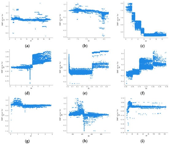
Figure 4.
Single-factor dependence plots for all data: (a) X1, (b) X2, (c) X3, (d) X4, (e) X5, (f) X6, (g) X7, (h) X8, and (i) X9.
Figure 4 shows that the SHAP values for water temperature (X1), pH (X2), TN (X7), and turbidity (X9) are centered around zero with little variation, indicating these factors have minimal impact on water quality and no distinct positive or negative correlation. This mirrors the findings in Figure 2.
When the DO concentration (X3) is low, the SHAP value increases, suggesting that low oxygen levels may negatively affect water quality. Conversely, at high DO concentrations, the SHAP value decreases, often becoming negative, indicating a beneficial impact on water quality.
Most SHAP values for the CODMn (X4) are positive, suggesting a significant negative impact on water quality. A few data points show negative SHAP values, but this does not imply a positive effect. The CODMn measures the oxidizable reducing substances, primarily organic pollutants, in water. Negative SHAP values may result from the interplay of various factors. Additionally, NH3-N (X5) and TP (X6) also exhibit a notable negative impact on water quality.
Regarding conductivity (X8), the scatter plot reveals no clear linear relationship or fixed pattern, suggesting that its influence on water quality prediction is likely complex and nonlinear.
3.5. Seasonal Dependency Graphs of Water Quality Influencing Factors
The dependency relationships of individual influencing factors for each season are further analyzed. Figure 5, Figure 6, Figure 7 and Figure 8 present the dependency graphs for the influencing factors across spring, summer, autumn, and winter.
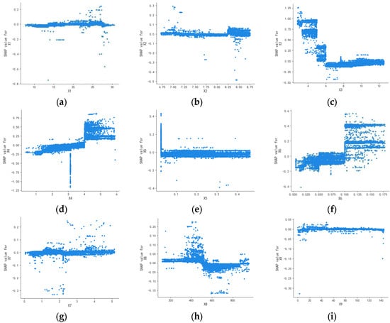
Figure 5.
Single-factor dependence plots for spring: (a) X1, (b) X2, (c) X3, (d) X4, (e) X5, (f) X6, (g) X7, (h) X8, and (i) X9.
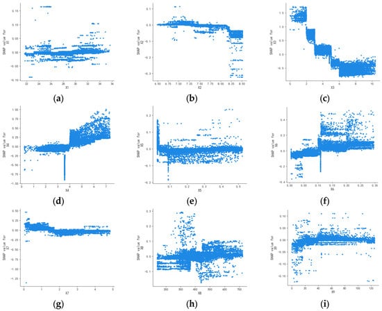
Figure 6.
Single-factor dependence plots for summer: (a) X1, (b) X2, (c) X3, (d) X4, (e) X5, (f) X6, (g) X7, (h) X8, and (i) X9.
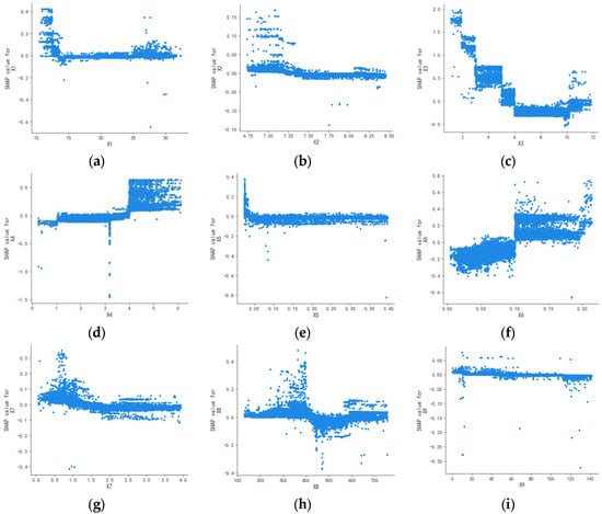
Figure 7.
Single-factor dependence plots for autumn: (a) X1, (b) X2, (c) X3, (d) X4, (e) X5, (f) X6, (g) X7, (h) X8, and (i) X9.
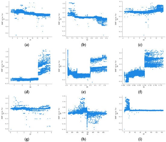
Figure 8.
Single-factor dependence plots for winter: (a) X1, (b) X2, (c) X3, (d) X4, (e) X5, (f) X6, (g) X7, (h) X8, and (i) X9.
Figure 5, Figure 6, Figure 7 and Figure 8 illustrate that the SHAP values for water temperature (X1), pH (X2), TN (X7), and turbidity (X9) consistently hover around zero with minimal seasonal variation. This suggests that these factors exert negligible influence on water quality, lacking any clear positive or negative correlation. This is basically consistent with the analysis results in Figure 2 and Figure 4.
The influence of DO (X3) on water quality during spring, summer, and autumn is consistent with the analysis in Figure 3, demonstrating a significant impact across these seasons. During these times, the SHAP values for DO (X3) exhibit considerable variation, underscoring its substantial role in water quality. Conversely, in winter, the SHAP values for DO (X3) are concentrated around zero with minimal variation, suggesting it is not a major factor in water quality. This is due to lower water temperatures in winter, which diminish biological activity and, consequently, the consumption of DO.
The conclusions derived from the CODMn (X4) and conductivity (X8) across the four seasons align with those depicted in Figure 4.
NH3-N (X5) exerts minimal influence on water quality in spring and autumn, showing no clear correlation. In summer, despite SHAP values clustering around zero, there is a slightly wider range compared to spring and autumn, indicating a relatively greater impact on water quality. In winter, as NH3-N concentration rises, its effect on water quality shifts from negative to positive, becoming more pronounced at higher concentrations. The wide range of SHAP values suggests that in winter, due to reduced biological activity, both the release and absorption of NH3-N decrease, leading to a stable concentration and significant impact on water quality, consistent with the findings in Figure 3.
The impact of TP (X6) on water quality remains consistent throughout the seasons, lacking a clear linear relationship. As TP concentration rises, the SHAP value also increases, shifting its effect on water quality from positive to negative and leading to a deterioration in water quality. This finding aligns with the results depicted in Figure 2, Figure 3 and Figure 4.
4. Conclusions
This study integrates the XGBoost model with the SHAP interpretation framework to predict water quality in the Tai Lake Basin and identify key influencing factors. XGBoost, known for its efficiency and robustness, excels in handling large datasets and delivering accurate predictions. However, while models like XGBoost offer high predictive performance, they often lack interpretability, obscuring the impact of individual factors on predictions. To address this, the SHAP framework is employed to elucidate the XGBoost model’s results. It quantifies each factor’s contribution to water quality outcomes and provides a dependency graph, clearly illustrating the relationship between factor values and model outputs, thereby aiding in the assessment of each factor’s relative importance.
Comparative analysis of factor dependence graphs elucidated the interactions between factors and their effects on model predictions. These graphs enhance comprehension of the model’s internal mechanisms and serve as valuable references for water quality prediction and management. The study assessed factor contributions across the entire dataset and compared seasonal indicator data to reveal how seasonal changes impact factor contributions. This approach aids in accurately interpreting the influence of various factors on water quality across different seasons.
The primary conclusions are as follows: (1) During spring, summer, and autumn in the Tai Lake Basin, the key factors affecting water quality are DO (X3), TP (X6), and the CODMn (X4). DO (X3) positively influences water quality, whereas higher levels of TP (X6) and the CODMn (X4) negatively impact it. (2) In winter, DO is not a major factor; instead, TP (X6), NH3-N (X5), and the CODMn (X4) are the main influences, all adversely affecting water quality. (3) Compared to these factors, water temperature (X1), pH (X2), TN (X7), and turbidity (X9) exhibit minimal seasonal variation and have a negligible impact on water quality, showing no clear positive or negative correlation.
Human activities, livestock, and poultry farming activities are significantly correlated with the water quality of Tai Lake [53]. Therefore, this study puts forward the following policy recommendations.
In spring, summer, and autumn, the primary influencing factors are DO, TP, and CODMn. For DO, given that water temperature, atmospheric pressure, and salinity impact its levels, regulating water temperature is crucial. In high-temperature summers, strategies such as enhancing water flow and constructing shading facilities can help reduce water temperature and thereby increase DO. Additionally, salinity should be managed to prevent it from lowering DO levels. Regarding TP, it is essential to monitor the growth rate of aquatic plants like algae during these seasons. Excessive plant growth can elevate TP levels, necessitating regular removal of these plants to control their proliferation. Concurrently, sewage treatment should be enhanced to minimize phosphorus emissions. In spring, summer, and autumn, elevated water temperatures increase the degradation rate of organic matter, potentially resulting in high organic content in water bodies, as indicated by the CODMn. To address this, the sewage treatment process must be optimized to enhance organic matter removal. Additionally, stricter management of agricultural and urban sewage is necessary to minimize the discharge of pesticides, fertilizers, and organic matter.
In winter, unlike the other seasons, TP, NH3-N, and CODMn are the primary influencing factors, all exerting negative effects. The low winter temperatures reduce biological activity, potentially resulting in excess phosphorus in treated water. To manage this, sewage treatment plants can enhance operations, optimize biochemical processes, and employ high-efficiency phosphorus-removing flocculants alongside conventional chemical and biochemical methods to maintain phosphorus levels within acceptable limits. NH3-N has been identified as a primary stressor in the catchment of the eutrophic Tai Lake in China, contributing to declines in benthic invertebrate diversity [54,55]. Consequently, reducing NH3-N concentrations is crucial. In winter, the activity of nitrifying bacteria decreases, impairing NH3-N removal efficiency. This can be mitigated by extending sludge age, reducing sludge discharge in oxidation ditches, and increasing sludge concentration. Additionally, the low winter water temperatures slow the degradation of organic matter, potentially increasing the CODMn. Optimizing the sewage treatment process may improve the removal rate of organic matter.
For factors of lesser importance, integrated management should accompany the primary measures. Water temperature, particularly during summer and winter, requires enhanced monitoring. By adjusting reservoir discharge and increasing water fluidity, temperature fluctuations can be controlled, minimizing their impact on water quality. Regular monitoring of pH levels is essential to maintain them within an optimal range. Deviations can be corrected with acid–base neutralizers, and sources of change, such as industrial wastewater, must be addressed. Conductivity, indicative of ion concentration, can be reduced by controlling ion sources, such as limiting fertilizers and pesticides, and improving wastewater treatment. High turbidity, which affects water transparency, can be managed by controlling soil erosion to limit sediment influx and enhancing sedimentation and filtration processes to reduce suspended particulates.
The sustainable development of water resources in the Tai Lake Basin is crucial for the economic and social advancement of the Yangtze River region and China [56]. To address key influencing factors, it is essential to enhance the water quality monitoring network in the Tai Lake Basin, increasing both the frequency and accuracy of monitoring to swiftly identify and resolve water quality issues. Concurrently, the development and enforcement of water quality management regulations should be strengthened, with clear delineation of departmental responsibilities and authority to ensure effective implementation of water quality treatment efforts.
Author Contributions
W.L. contributed to data curation, investigation, project administration, software, writing—original draft, and writing—review and editing. M.D. contributed to conceptualization, methodology, and validation. C.L. contributed to data curation, formal analysis, software, and writing—original draft. Q.C. contributed to supervision and writing—review and editing. All authors have read and agreed to the published version of the manuscript.
Funding
This research was funded by the Key R&D projects in Ningxia Autonomous Region (2023BEG02054).
Data Availability Statement
The data presented in this study are available on request from the corresponding author.
Conflicts of Interest
The authors declare no conflicts of interest.
References
- Cotruvo, J.A. 2017 WHO Guidelines for Drinking Water Quality: First Addendum to the Fourth Edition. J. Am. Water Work. Assoc. 2017, 109, 44–51. [Google Scholar] [CrossRef]
- Huan, J.; Fan, Y.X.; Xu, X.G.; Zhou, L.W.; Zhang, H.; Zhang, C.; Hu, Q.C.; Cai, W.X.; Ju, H.R.; Gu, S.L. Deep learning model based on coupled SWAT and interpretable methods for water quality prediction under the influence of non-point source pollution. Comput. Electron. Agric. 2025, 231, 109985. [Google Scholar] [CrossRef]
- Liao, H.B.; Yuan, L.; Wu, M.; Chen, H.S. Air quality prediction by integrating mechanism model and machine learning model. Sci. Total Environ. 2023, 899, 165646. [Google Scholar] [CrossRef]
- LeCun, Y.; Bengio, Y.; Hinton, G. Deep learning. Nature 2015, 521, 436–444. [Google Scholar] [CrossRef]
- Streeter, H.W.; Phclps, E.B. A Study of the Pollution and Natural Purification of the Ohio River. U.S. Public Hcaith Bull. 1925, 146, 1–75. [Google Scholar]
- Paliwal, R.; Sharma, P.; Kansal, A. Water quality modelling of the river Yamuna (India) using QUAL2E-UNCAS. J. Environ. Manag. 2007, 83, 131–144. [Google Scholar] [CrossRef]
- Costa, C.; Marques, L.D.; Almeida, A.K.; Leite, I.R.; de Almeida, I.K. Applicability of water quality models around the world-a review. Environ. Sci. Pollut. Res. 2019, 26, 36141–36162. [Google Scholar] [CrossRef]
- Arnold, J.G.; Srinivasan, R.; Muttiah, R.S.; Williams, J.R. Large area hydrologic modeling and assessment part I: Model development. Jawra 1998, 34, 73–89. [Google Scholar] [CrossRef]
- Wan, H.; Xu, R.; Zhang, M.; Cai, Y.P.; Li, J.; Shen, X. A novel model for water quality prediction caused by non-point sources pollution based on deep learning and feature extraction methods. J. Hydrol. 2022, 612, 128081. [Google Scholar] [CrossRef]
- Cui, Q.; Wang, X.; Li, C.H.; Cai, Y.P.; Liang, P.Y. Improved Thomas-Fiering and wavelet neural network models for cumulative errors reduction in reservoir inflow forecast. J. Hydro-Environ. Res. 2016, 13, 134–143. [Google Scholar] [CrossRef]
- Zhang, Q.Q.; Li, Z.; Zhu, L.; Zhang, F.; Sekerinski, E.; Han, J.C.; Zhou, Y. Real-time prediction of river chloride concentration using ensemble learning. Environ. Pollut. 2021, 291, 118116. [Google Scholar] [CrossRef] [PubMed]
- Shaw, A.R.; Sawyer, H.S.; LeBoeuf, E.J.; McDonald, M.P.; Hadjerioua, B. Hydropower Optimization Using Artificial Neural Network Surrogate Models of a High-Fidelity Hydrodynamics and Water Quality Model. Water Resour. Res. 2017, 53, 9444–9461. [Google Scholar] [CrossRef]
- Aliashrafi, A.; Zhang, Y.R.; Groenewegen, H.; Peleato, N.M. A review of data-driven modelling in drinking water treatment. Rev. Environ. Sci. Bio-Technol. 2021, 20, 985–1009. [Google Scholar] [CrossRef]
- Rajaee, T.; Khani, S.; Ravansalar, M. Artificial intelligence-based single and hybrid models for prediction of water quality in rivers: A review. Chemom. Intell. Lab. Syst. 2020, 200, 103978. [Google Scholar] [CrossRef]
- Noori, N.; Kalin, L.; Isik, S. Water quality prediction using SWAT-ANN coupled approach. J. Hydrol. 2020, 590, 125220. [Google Scholar] [CrossRef]
- Samsudin, M.S.; Azid, A.; Khalit, S.I.; Sani, M.S.A.; Lananan, F. Comparison of prediction model using spatial discriminant analysis for marine water quality index in mangrove estuarine zones. Mar. Pollut. Bull. 2019, 141, 472–481. [Google Scholar] [CrossRef]
- Ta, X.X.; Wei, Y.G. Research on a dissolved oxygen prediction method for recirculating aquaculture systems based on a convolution neural network. Comput. Electron. Agric. 2018, 145, 302–310. [Google Scholar] [CrossRef]
- Lundberg, S.M.; Lee, S.I. In A Unified Approach to Interpreting Model Predictions. In Proceedings of the 31st Annual Conference on Neural Information Processing Systems (NIPS), Long Beach, CA, USA, 4–9 December 2017. [Google Scholar]
- Lubo-Robles, D.; Devegowda, D.; Jayaram, V.; Bedle, H.; Marfurt, K.J.; Pranter, M.J. Quantifying the sensitivity of seismic facies classification to seismic attribute selection: An explainable machine-learning study. Interpret.-A J. Subsurf. Charact. 2022, 10, SE41–SE69. [Google Scholar] [CrossRef]
- Batunacun; Wieland, R.; Lakes, T.; Nendel, C. Using Shapley additive explanations to interpret extreme gradient boosting predictions of grassland degradation in Xilingol, China. Geosci. Model Dev. 2021, 14, 1493–1510. [Google Scholar] [CrossRef]
- Niazkar, M.; Menapace, A.; Brentan, B.; Piraei, R.; Jimenez, D.; Dhawan, P.; Righetti, M. Applications of XGBoost in water resources engineering: A systematic literature review (Dec 2018-May 2023). Environ. Model. Softw. 2024, 174, 105971. [Google Scholar] [CrossRef]
- Morita, K.; Davies, D.W.; Butler, K.T.; Walsh, A. Modeling the dielectric constants of crystals using machine learning. J. Chem. Phys. 2020, 153, 024503. [Google Scholar] [CrossRef] [PubMed]
- Merabet, K.; Di Nunno, F.; Granata, F.; Kim, S.; Adnan, R.M.; Heddam, S.; Kisi, O.; Zounemat-Kermani, M. Predicting water quality variables using gradient boosting machine: Global versus local explainability using SHapley Additive Explanations (SHAP). Earth Sci. Inform. 2025, 18, 298. [Google Scholar] [CrossRef]
- Kruk, M. SHAP-NET, a network based on Shapley values as a new tool to improve the explainability of the XGBoost-SHAP model for the problem of water quality. Environ. Model. Softw. 2025, 188, 106403. [Google Scholar] [CrossRef]
- Park, J.; Lee, W.H.; Kim, K.T.; Park, C.Y.; Lee, S.; Heo, T.Y. Interpretation of ensemble learning to predict water quality using explainable artificial intelligence. Sci. Total Environ. 2022, 832, 155070. [Google Scholar] [CrossRef] [PubMed]
- Huang, J.; Wang, X.X.; Xi, B.D.; Xu, Q.J.; Tang, Y.; Jia, K.L.; Mao, J.Y. Long-term variations of TN and TP in four lakes fed by Yangtze River at various timescales. Environ. Earth Sci. 2015, 74, 3993–4009. [Google Scholar] [CrossRef]
- Li, C.C.; Feng, W.Y.; Song, F.H.; He, Z.Q.; Wu, F.C.; Zhu, Y.R.; Bai, Y.C. Three decades of changes in water environment of a large freshwater Lake and its relationship with socio-economic indicators. J. Environ. Sci. 2019, 77, 156–166. [Google Scholar] [CrossRef]
- Tan, R.; Wang, Z.; Wu, T.; Wu, J. A data-driven model for water quality prediction in Tai Lake, China, using secondary modal decomposition with multidimensional external features. J. Hydrol.-Reg. Stud. 2023, 47, 101435. [Google Scholar] [CrossRef]
- Xu, R.; Pang, Y.; Hu, Z.; Hu, X. The Spatiotemporal Characteristics of Water Quality and Main Controlling Factors of Algal Blooms in Tai Lake, China. Sustainability 2022, 14, 5710. [Google Scholar] [CrossRef]
- Zhou, J.; Wang, Y.; Xiao, F.; Wang, Y.; Sun, L. Water Quality Prediction Method Based on IGRA and LSTM. Water 2018, 10, 1148. [Google Scholar] [CrossRef]
- Sun, G.; Zhu, W.; Qian, X.; Wei, C.; Xie, P.; Shi, Y.; Cao, X.; He, Y. Machine Learning Models for Chlorophyll-a Forecasting in a Freshwater Lake: Case Study of Lake Taihu. Water 2025, 17, 1219. [Google Scholar] [CrossRef]
- Ananias, P.H.M.; Negri, R.G.; Dias, M.A.; Silva, E.A.; Casaca, W. A Fully Unsupervised Machine Learning Framework for Algal Bloom Forecasting in Inland Waters Using MODIS Time Series and Climatic Products. Remote Sens. 2022, 14, 4283. [Google Scholar] [CrossRef]
- Chen, X.Z.; Jia, J.F.; Bai, Y.L.; Guo, T.; Du, X.L. Prediction model of axial bearing capacity of concrete-filled steel tube columns based on XGBoost-SHAP. J. Zhejiang Univ. Eng. Sci. 2023, 57, 1061–1070. [Google Scholar]
- Ahmadi, S.M.; Balahang, S.; Abolfathi, S. Predicting the hydraulic response of critical transport infrastructures during extreme flood events. Eng. Appl. Artif. Intell. 2024, 133, 108573. [Google Scholar] [CrossRef]
- Elith, J.; Leathwick, J.R.; Hastie, T. A working guide to boosted regression trees. J. Anim. Ecol. 2008, 77, 802–813. [Google Scholar] [CrossRef]
- Chen, T.; Guestrin, C. XGBoost: A scalable tree boosting system. In Proceedings of the 22nd ACM SIGKDD International Conference on Knowledge Discovery and Data Mining—KDD ’16, San Francisco, CA, USA, 13–17 August 2016; pp. 785–794. [Google Scholar]
- Friedman, J.H. Greedy function approximation: A gradient boosting machine. Ann. Stat. 2001, 29, 1189–1232. [Google Scholar] [CrossRef]
- Wang, Y.H.; Wang, L.Q.; Liu, S.L.; Liu, P.F.; Zhu, Z.W.; Zhang, W.A. A comparative study of regional landslide susceptibility mapping with multiple machine learning models. Geol. J. 2024, 59, 2383–2400. [Google Scholar] [CrossRef]
- Choi, D.K. Data-Driven Materials Modeling with XGBoost Algorithm and Statistical Inference Analysis for Prediction of Fatigue Strength of Steels. Int. J. Precis. Eng. Manuf. 2019, 20, 129–138. [Google Scholar] [CrossRef]
- Shapley, L.S. A Value for n-Person Games; Princeton University Press: Princeton, NJ, USA, 1953; pp. 307–318. [Google Scholar]
- Zhang, J.; Ma, X.; Zhang, J.; Sun, D.; Zhou, X.; Mi, C.; Wen, H. Insights into geospatial heterogeneity of landslide susceptibility based on the SHAP-XGBoost model. J. Environ. Manag. 2023, 332, 117357. [Google Scholar] [CrossRef]
- Li, Z.Q. Extracting spatial effects from machine learning model using local interpretation method: An example of SHAP and XGBoost. Comput. Environ. Urban Syst. 2022, 96, 101845. [Google Scholar] [CrossRef]
- Feng, D.C.; Wang, W.J.; Mangalathu, S.; Taciroglu, E. Interpretable XGBoost-SHAP Machine-Learning Model for Shear Strength Prediction of Squat RC Walls. J. Struct. Eng. 2021, 147, 04021173. [Google Scholar] [CrossRef]
- Pan, B.; Song, T.R.; Yue, M.; Chen, S.N.; Zhang, L.J.; Edlmann, K.; Neil, C.W.; Zhu, W.Y.; Iglauer, S. Machine learning- based shale wettability prediction: Implications for H2, CH4 and CO2 geo-storage. Int. J. Hydrogen Energy 2024, 56, 1384–1390. [Google Scholar] [CrossRef]
- Yin, Z.Y.; Li, J.S.; Liu, Y.; Xie, Y.; Zhang, F.F.; Wang, S.L.; Sun, X.; Zhang, B. Water clarity changes in Lake Taihu over 36 years based on Landsat TM and OLI observations. Int. J. Appl. Earth Obs. Geoinf. 2021, 102, 102457. [Google Scholar] [CrossRef]
- Liu, Z.F.; Ying, J.H.; He, C.Y.; Guan, D.J.; Pan, X.H.; Dai, Y.H.; Gong, B.H.; He, K.R.; Lv, C.F.; Wang, X.; et al. Scarcity and quality risks for future global urban water supply. Landsc. Ecol. 2024, 39, 10. [Google Scholar] [CrossRef]
- Wu, Y.X.; Jiang, L.L.; Ouyang, X.T.; Wang, Z.L.; Jiang, Q.X. Sustainable evaluation of the water footprint in Heilongjiang Province, China, based on correlation-matter element analysis. J. Clean. Prod. 2023, 408, 137231. [Google Scholar] [CrossRef]
- Joharestani, M.Z.; Cao, C.X.; Ni, X.L.; Bashir, B.; Talebiesfandarani, S. PM2.5 Prediction Based on Random Forest, XGBoost, and Deep Learning Using Multisource Remote Sensing Data. Atmosphere 2019, 10, 373. [Google Scholar] [CrossRef]
- Fang, L.; Shi, X.F.; Pan, R.J.; Wu, Q. Water quality characteristic analysis about three different types of surface drinking water sources: A study case of Huzhou, China. Fresenius Environ. Bull. 2017, 26, 969–976. [Google Scholar]
- Hu, Q. Analysis and Comprehensive Evaluation of Taihu Lake Water Quality from 2011 to 2020. J. Shantou Univ. (Nat. Sci. Ed.) 2022, 37, 65–74. [Google Scholar]
- Zhu, G.W. Spatiotemporal Variations of Taihu Lake Water Quality and Its Relationship with Algal Blooms. Resour. Environ. Yangtze River Basin 2009, 18, 439–445. [Google Scholar]
- Environmental Quality Standards for Surface Water. Available online: https://www.mee.gov.cn/ywgz/fgbz/bz/bzwb/shjbh/shjzlbz/200206/t20020601_66497.shtml (accessed on 13 May 2025).
- Lian, H.S.; Liu, H.B.; Li, X.D.; Song, T.; Lei, Q.L.; Ren, T.Z.; Li, Y. Analysis of Spatial Variability of Water Quality and Pollution Sources in Lihe River Watershed, Taihu Lake Basin. Environ. Sci. 2017, 38, 3657–3665. [Google Scholar]
- Li, Y.B.; Xu, E.G.; Liu, W.; Chen, Y.; Liu, H.L.; Li, D.; Yu, H.X. Spatial and temporal ecological risk assessment of unionized ammonia nitrogen in Tai Lake, China (2004-2015). Ecotoxicol. Environ. Saf. 2017, 140, 249–255. [Google Scholar] [CrossRef]
- Yang, J.H.; Zhang, X.W.; Xie, Y.W.; Song, C.; Sun, J.Y.; Zhang, Y.; Yu, H.X. Ecogenomics of Zooplankton Community Reveals Ecological Threshold of Ammonia Nitrogen. Environ. Sci. Technol. 2017, 51, 3057–3064. [Google Scholar] [CrossRef]
- Peng, Q.L.; He, W.J.; Kong, Y.; Shen, J.Q.; Yuan, L.; Ramsey, T.S. Spatio-temporal analysis of water sustainability of cities in the Yangtze River Economic Belt based on the perspectives of quantity-quality-benefit. Ecol. Indic. 2024, 160, 111909. [Google Scholar] [CrossRef]
Disclaimer/Publisher’s Note: The statements, opinions and data contained in all publications are solely those of the individual author(s) and contributor(s) and not of MDPI and/or the editor(s). MDPI and/or the editor(s) disclaim responsibility for any injury to people or property resulting from any ideas, methods, instructions or products referred to in the content. |
© 2025 by the authors. Licensee MDPI, Basel, Switzerland. This article is an open access article distributed under the terms and conditions of the Creative Commons Attribution (CC BY) license (https://creativecommons.org/licenses/by/4.0/).