High-Resolution Water Quality Monitoring of Small Reservoirs Using UAV-Based Multispectral Imaging

Abstract

Multispectral satellite imagery has been widely applied in water quality monitoring, but limitations in spatial–temporal resolution and acquisition delays often hinder accurate assessments in small water bodies. In this study, a DJI M600PRO UAV equipped with a Sequoia multispectral sensor was used to assess the water quality in Zhangshan Reservoir, a small inland reservoir in Chuzhou, Anhui, China. Two regression approaches—the Window Averaging Method (WAM) and the Matching Pixel-by-Pixel Method (MPP)—were used to link UAV-derived spectral indices with in situ measurements of total nitrogen (TN), total phosphorus (TP), and chemical oxygen demand (COD). Despite a limited sample size (n = 60) and single-day sampling, MPP outperformed WAM, achieving higher predictive accuracy (R² = 0.970 for TN, 0.902 for TP, and 0.695 for COD). The findings demonstrate that UAV-based MPP effectively captures fine-scale spatial heterogeneity and offers a promising solution for monitoring water quality in small and turbid reservoirs, overcoming key limitations of satellite-based remote sensing. However, the study is constrained by the temporal coverage and sample density, and future work should integrate multi-temporal UAV observations and expand the dataset to improve the model robustness and generalizability.

1. Introduction

With the rapid pace of economic and social development in China, urbanization, industrialization, and agricultural intensification have significantly intensified conflicts between human activities and natural water resources [1]. Under dual pressures of water scarcity and escalating pollution [2], safeguarding aquatic environments and ensuring effective water quality monitoring have become central goals in China’s ecological civilization initiatives [3]. Small reservoirs play a vital role in supplying rural drinking water, supporting agricultural irrigation, and conserving ecosystems [4]. Their water quality directly impacts public health, agricultural productivity, and the stability of local ecosystems. China has a large number of small reservoirs (typically < 1 km²), many located in mountainous or hilly terrain [5]. These water bodies show high spatial heterogeneity, but traditional point-based monitoring is inefficient, expensive, and poorly suited for dynamic, high-resolution mapping [6,7,8].

In response, remote sensing technologies have gained traction in water quality monitoring due to their wide spatial coverage, non-invasive nature, and high spatiotemporal resolution [9]. Over recent decades, satellite-based remote sensing has become a mainstream tool for regional-scale water quality assessment [10]. For example, the Landsat series has provided continuous multispectral imagery since 1972 [11]. Its visible, near-infrared, and thermal infrared bands have been extensively used to retrieve parameters such as suspended solids, chlorophyl ll-a, and turbidity through empirical modeling [12,13,14]. Studies by Baban [15] and Kulkarni [16] demonstrated successful retrieval of water quality indicators in the UK and the US, while Bonansea, et al. [17] and Chen, et al. [18] employed Landsat data to estimate lake transparency and nutrient concentrations and evaluate atmospheric correction methods. Many studies have shown that an increase in the total phosphorus concentration in water bodies leads to a general increase in the chlorophyll a concentration [19]. For instance, Song et al. used selected sensitive spectral variables to conduct remote sensing estimations of total phosphorus (TP), chlorophyll a (Chl-a), and saturated sea surface area (SDT) [20].

In addition to satellite and UAV-based remote sensing, in situ sensor technologies—such as wireless sensor networks (WSNs) and IoT-based platforms—are increasingly being deployed in freshwater monitoring. These systems offer real-time, high-frequency observations and have proven effective in capturing dynamic changes in water quality parameters, especially when integrated with remote sensing data. For instance, Singh and Walingo developed a smart water quality monitoring framework that combines IoT and WSN technologies with artificial intelligence to predict parameters like E. coli concentrations, demonstrating the potential of such integrated systems in enhancing water quality monitoring efforts [21].

Despite these advancements, satellite-based approaches face several limitations. Their utility is constrained by long revisit cycles (e.g., 16 days for Landsat) and weather dependency, which affect data timeliness and consistency [22]. Additionally, their typical 30 m spatial resolution is insufficient for delineating narrow water bodies, and they are prone to mixed-pixel contamination from adjacent land features such as vegetation or bare soil [23,24]. Moreover, empirical models developed using satellite data often lack generalizability across different regions due to seasonal and spatial variability in water quality parameters. These challenges are especially pronounced for the retrieval of non-optically active parameters such as total nitrogen (TN) and total phosphorus (TP), which exhibit weak spectral signals and are difficult to model accurately [25].

To address the resolution and latency challenges of traditional remote sensing in small water body monitoring, unmanned aerial vehicle (UAV) remote sensing has emerged as a promising alternative [26]. UAV platforms offer ultra-high spatial resolution, low-altitude operation, flexible deployment schedules, and relatively low operational costs. Equipped with diverse sensors—including multispectral, red-edge, hyperspectral, and thermal infrared—UAVs enable customized, high-precision monitoring tailored to specific study areas. Unlike satellite sensors, UAVs are not hindered by cloud cover and can collect data under optimal environmental conditions, making them particularly suitable for complex terrains and small-scale water bodies [9].

Studies have shown that UAV imagery at centimeter-level resolution can effectively capture spatial heterogeneity and reduce mixed-pixel errors, thereby enhancing the accuracy of water quality retrievals [27,28]. Cillero Castro, et al. [27] proposed an integrated framework combining UAV and satellite data for assessing the trophic status of small drinking water reservoirs. Liu, et al. [29] integrated UAV-based multispectral imagery with machine learning algorithms (e.g., XGBoost, CatBoost), substantially improving the retrieval accuracy of chlorophyll-a and turbidity while mapping their spatiotemporal patterns. UAVs also offer rapid data acquisition and flexible scheduling, enabling multi-temporal monitoring and emergency response applications. Their high spatial fidelity ensures strong alignment between pixel values and ground-truth samples, which facilitates better model fitting and enhances predictive performance [29].

Additionally, new modeling approaches have been developed to improve the robustness and efficiency of UAV-based water quality estimation, such as matching pixel-by-pixel (MPP) [30,31], partial least squares regression (PLSR) [32], Multiple Linear Regression, the Least Absolute Shrinkage and Selection Operator, Backpropagation Neural Network (BP), Random Forest (RF), and eXtreme Gradient Boosting (XGBoost) [33,34], which have been used to estimating water quality parameters like TN, TP, and chemical oxygen demand (COD).

In summary, UAV-based multispectral remote sensing provides an effective mid-scale solution that bridges the gap between field sampling and satellite observation, offering considerable potential for monitoring water quality in small reservoirs. However, systematic research on the quantitative retrieval of non-optically active parameters (e.g., dissolved organic matter and nutrients) remains limited. Furthermore, constructing robust, multi-source fusion models that can reliably adapt to diverse environmental conditions is still a major research need. To answer this question, high-resolution imagery was collected from the Zhangshan Reservoir in Dingyuan County, Anhui Province, using a DJI M600 Pro UAV with a Parrot Sequoia multispectral camera. Simultaneously, surface water samples were analyzed for TN, TP, and COD. Statistical models were built to evaluate the relationships between spectral indices and water quality indicators, aiming to assess retrieval accuracy and spatial patterns. This study offers a practical and scalable method for estimating nutrient-related water quality indicators in small water bodies with limited in situ data. By integrating spatial window-based regression approaches with UAV multispectral imagery, it provides a novel contribution to fine-scale water quality monitoring and model development under data-constrained scenarios.

2. Study Area and Methodology

2.1. Study Area

Zhangshan Reservoir is situated in Beizhangzhuang Village, Xisadian Town, in the northwestern part of Dingyuan County, Chuzhou City, Anhui Province, China. The reservoir spans an area of approximately 0.34 km² and has a total storage capacity of about 2.44 million cubic meters. It lies between latitudes 32°36′57″ N and 32°37′18″ N and longitudes 117°31′5″ E and 117°31′42″E (Figure 1).

The reservoir infrastructure includes a dam, a spillway, and a drainage culvert. Upstream of the reservoir lies the Zhangshan Small Watershed Comprehensive Soil and Water Conservation Demonstration Base, established in 2017 by the Anhui Provincial Institute of Water Resources and Soil Conservation. This demonstration site features a 329.47 m long channel and eight runoff subzones designed for experimental and management purposes.

Downstream, the reservoir drains toward Zhangzhuang Village. The broader Zhangshan Basin encompasses state-owned forest areas such as Xiyang Mountain Forest Farm and Jiushan Livestock Farm. These areas are rich in rocky mountainous terrain and sloped grasslands, making them well suited for large-scale livestock operations. Zhangshan Reservoir plays a crucial role in supporting local agriculture and animal husbandry by providing irrigation water to downstream farmland and ensuring water supply to nearby farms and pastures. Its diverse land use and well-defined hydrological structure make it an ideal case study for small reservoir water quality research (see Figure 1).

On the sampling date—23 October 2019—the reservoir’s water level was recorded at 117.81 m at 8:00 AM, with a corresponding volume of 286,000 cubic meters (data source: http://yc.wswj.net/ahsxx/LOL/?refer=upl&to=public_public (accessed on 23 October 2019) [35]).

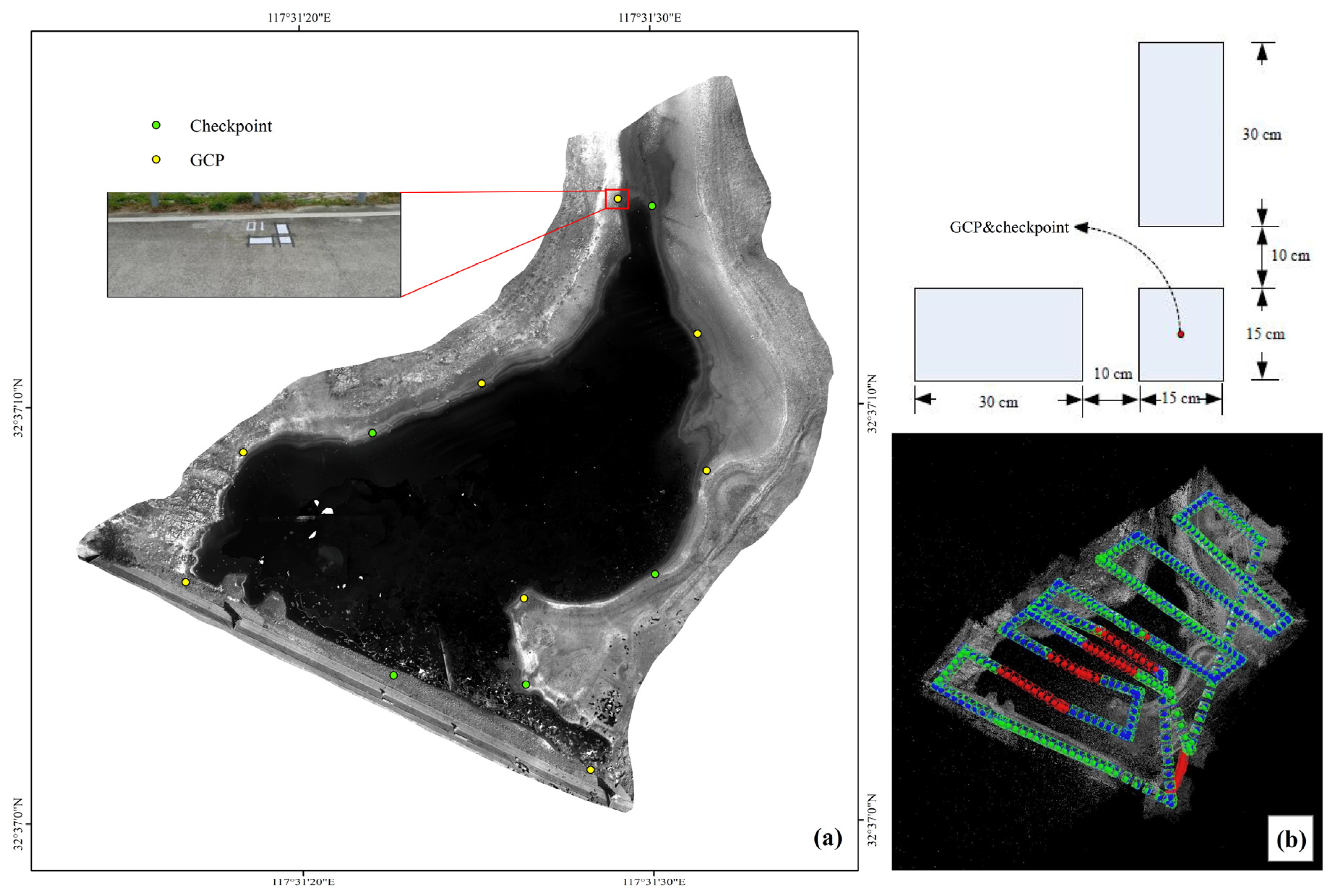
2.2. Field Measurement Data of the Reservoir

Higher nutrient concentrations—particularly TN—tend to promote the proliferation of plankton such as algae, which in turn reduces water transparency. Algal biomass and water clarity can be indirectly estimated by measuring the Chl-a concentration and Secchi disk depth (SD), respectively, both of which serve as important indicators of the trophic status in aquatic ecosystems.

On the morning of 23 October 2019, following UAV-based remote sensing data collection at Zhangshan Reservoir, water samples were collected from the reservoir and transported the same afternoon to the Xinmaqiao Experimental Station for laboratory analysis. This sampling schedule was designed to minimize temporal discrepancies between image acquisition and water quality measurements, thereby improving data reliability. For example, delays in sample processing, particularly in warm seasons without cold-chain transportation, may lead to elevated temperatures in the samples, potentially altering parameters such as COD.

A total of six sampling sites were established within the reservoir. The spatial distribution of the sampling sites is illustrated in Figure 1. At each sampling site, ten individual surface water samples were collected (from the top 0–20 cm) to capture spatial variability, resulting in a total of 60 samples. Sample locations were georeferenced using a real-time kinematic (RTK) handheld GPS with a positional accuracy of 0.01–0.3 m horizontally and 0.02–0.5 m vertically. For model development, five samples from each site (half of the data) were used. The remaining 30 samples were reserved for model validation, from which 10 samples were randomly selected to assess model accuracy. The literature indicates that the density of sampling points in reservoirs generally ranges from 0.01 to 2.34 points/km² [36]. In this study, the sampling density (6 points within 34 hectares = 17.65 points/km²) is sufficient to monitor such a small reservoir.

The higher the concentration of nutrients (e.g., TN) is, the greater the number of plankton, such as algae, and the lower the water transparency. Algal biomass and water transparency can be roughly estimated by measuring the concentration of Chl-a and SD of the water body, respectively. On the morning of 23 October 2019, after UAV image acquisition at Zhangshan Reservoir, water samples were simultaneously collected and sent to the Xinmaqiao Experimental Station in the afternoon for data analysis. This approach was adopted to avoid errors due to the time gap between image acquisition and water sample collection, as an extended interval could affect the sampling data. For instance, during summer, the lack of a refrigerated transport box could lead to elevated temperatures, causing an increase in parameters such as COD in the water samples.

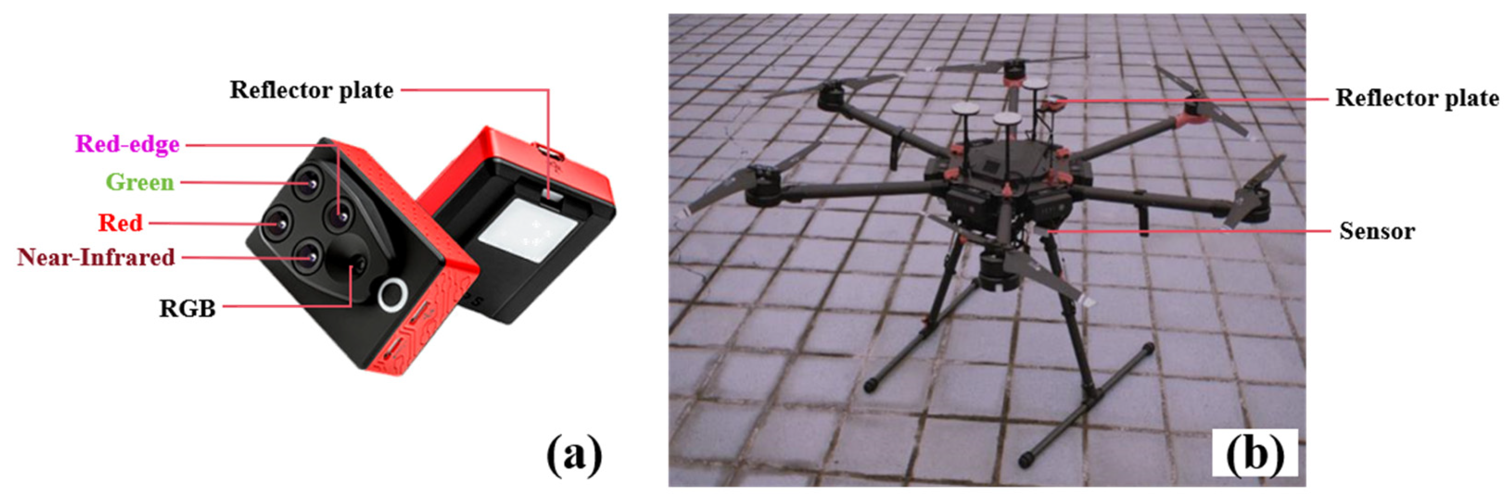
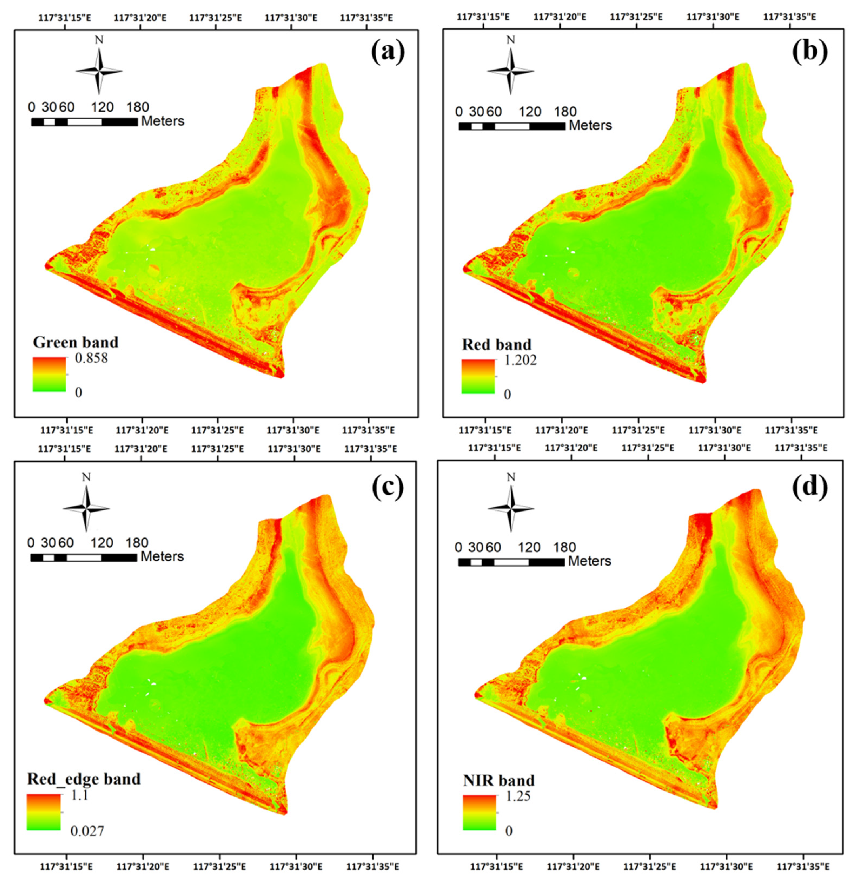
2.3. UAV System and Image Preprocessing

The UAV remote sensing system employed in this study was designed to capture multispectral imagery in four key spectral bands: green (G, 550 nm, bandwidth 40 nm), red (R, 660 nm, bandwidth 40 nm), red-edge (735 nm, bandwidth 10 nm), and near-infrared (NIR, 790 nm, bandwidth 40 nm). The images were recorded in TIFF format with embedded geolocation data. The multispectral sensor, weighing 72 g, features a built-in sunshine sensor (reflector plate) for automatic radiometric calibration. The sensor’s dimensions are 4.8 mm × 3.6 mm, and at a flight altitude of 100 m, the ground sampling distance (GSD) is approximately 0.12 m/pixel, with a focal length of 2.8 mm. The UAV system used is illustrated in Figure 2, which includes the Sequoia multispectral sensor (Parrot Company, Zug, Switzerland) and a multi-rotor DJI M600Pro (DJI, Hefei, China) platform.

To align UAV imagery with in situ measurements, ground control points (GCPs) were strategically placed during the image acquisition process to ensure geometric accuracy. A total of eight GCPs and five independent check points were distributed around the Zhangshan Reservoir, forming a precise geodetic control network essential for accurate photogrammetric mapping. GCPs were positioned between flight strips to optimize geometric correction. The spatial layout of the GCPs, check points, and UAV flight path is shown in Figure 2.

The imaging campaign covered approximately 42.8 hectares, during which 730 fixed-point images were captured in a single flight. UAV data acquisition occurred at 9:00 AM on 23 October 2019, under favorable environmental conditions: maximum temperature 22 °C, minimum temperature 12 °C, cloudy-to-overcast skies, northeast wind at level 2, and good visibility. The air quality index was 64 (data source: tianqi.2345.com (accessed on 23 October 2019)). The total flight time was 26 min with two flight passes. Flight parameters included an 80 m altitude, 10 m strip interval, 80% forward overlap, and 60% side overlap, yielding a strip coverage of 370 × 47 m². The pixel size was 7.36 cm, and each image had a resolution of 1280 × 960 pixels, generating a total of 2920 images across four spectral bands. Due to the low flight altitude (80 m), atmospheric effects on UAV imagery were considered negligible and thus not corrected. Previous studies have shown that UAV images acquired below 600 m typically exhibit minimal atmospheric interference, especially under stable weather conditions [37,38].

2.4. Image Preprocessing

Image preprocessing included mosaicking and geometric correction. Among the available UAV photogrammetry software platforms—such as Pix4Dmapper v4.5.2, 3Dsmart v4.4.15, PixelGrid v7.5, and Photoscan v1.0—Pix4Dmapper v4.5.2 was selected due to its robust support for aerial triangulation and high-precision mapping applications. The preprocessing workflow is illustrated in Figure 3 and Figure 4 and includes the following steps:

(1)

Input camera calibration data and TIFF images of the study area, including images of the reference calibration target and the four spectral bands.

(2)

Use the SIFT algorithm to detect and match feature points.

(3)

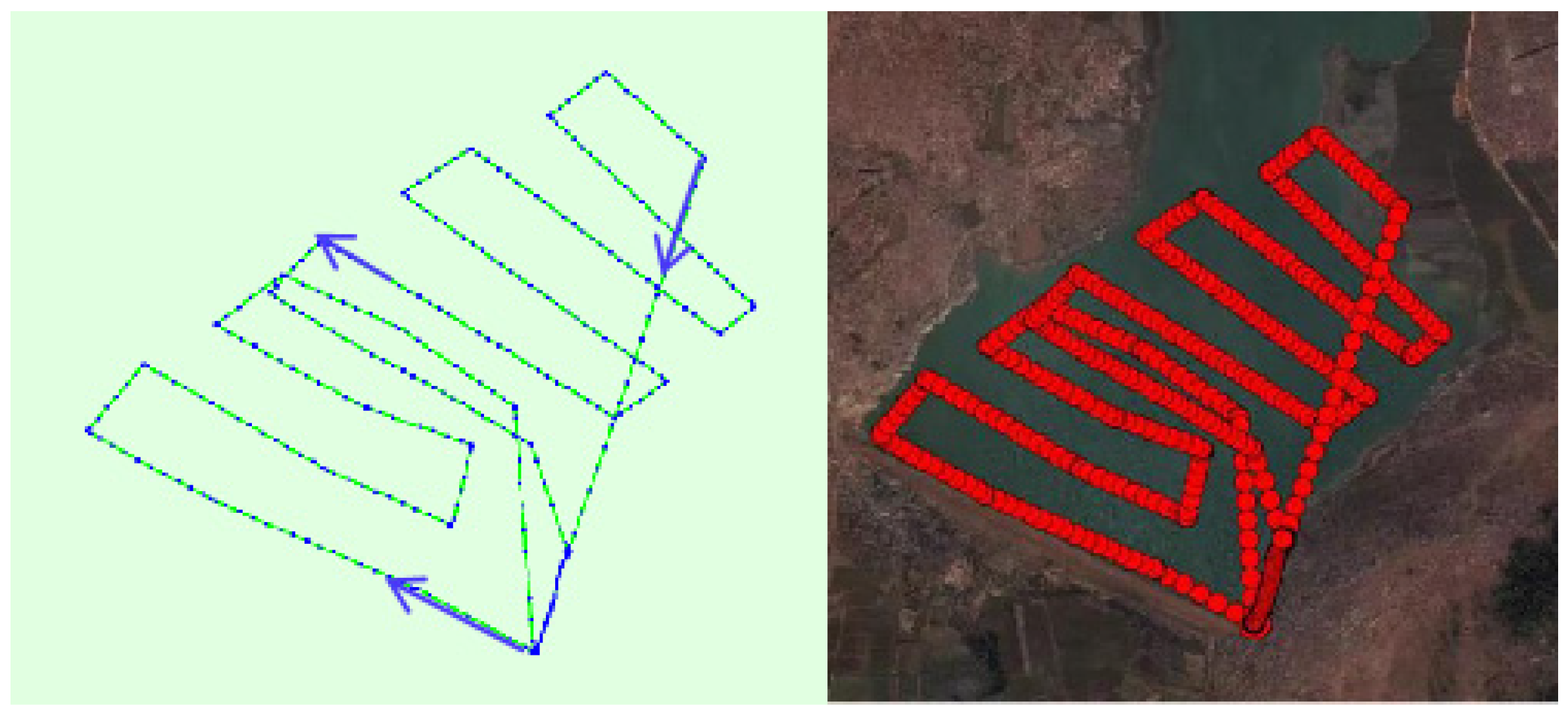
Perform spatial block adjustment using the matched features and embedded GPS data to restore image orientation.

(4)

Apply aerial triangulation using the GCPs to generate a 3D point cloud.

(5)

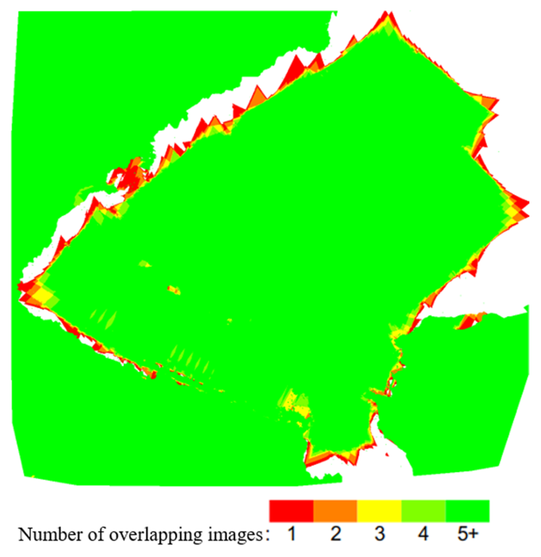
Produce a digital surface model (DSM) and a digital orthophoto map (DOM) from the point cloud data.

Figure 5 shows the overlap degree of the processed UAV images. Green represents areas covered by more than five images, while red indicates areas covered by only one image. To avoid errors caused by insufficient overlap and the inability to achieve proper stitching, it is necessary to ensure that more than five images are captured for the same location. The results in Figure 4 demonstrate that all the images within the reservoir area of the study region have more than five overlaps. After the images are stitched in Pix4Dmapper, they are imported into ArcGIS for geometric correction and coordinate system transformation, using ground control points. The study area is then cropped, and the image preprocessing results are shown in Figure 5.

After mosaicking, images were imported into ArcGIS 10.8 for geometric correction using the established GCP network. Coordinate system transformation and study area cropping were then conducted. The final preprocessed imagery for the green, red, red-edge, and NIR bands is shown in Figure 6.

2.5. Mapping Water Quality Parameters

Figure 7 presents the overall framework for mapping water quality parameters of Zhangshan Reservoir by integrating UAV multispectral imagery with field measurements. The primary objective is to establish regression models that accurately link spectral information (independent variables) with water quality indicators (dependent variables).

Establishing such models poses several challenges due to the complex nature of the water environment and variability in remote sensing data. Accordingly, this study evaluates multiple regression approaches—including linear, exponential, and logarithmic models—commonly used in water quality research. Statistical analysis was used to identify the most suitable relationships between the spectral reflectance or band ratios of image pixels and corresponding field measurements.

Compared to satellite imagery, UAV systems offer significantly higher spatial resolution. For example, an area represented by a single 10 × 10 m satellite pixel would correspond to over 10,000 UAV pixels. This allows UAV data to capture finer spatial variations, enabling more precise modeling and prediction of water quality. However, this high resolution introduces new challenges, such as selecting optimal pixels or window sizes for correlating imagery with field samples.

To address this, two statistical approaches were employed:

(1)

MPP: directly links individual image pixels with field measurements.

(2)

Window Averaging Method (WAM): uses averaged values over a defined window to reduce noise and account for local variability.

2.5.1. MPP Algorithm—Fixed Window Size, Search for Matching Within the Window

The MPP uses a buffer window of size n² × 0.07² square meters (where n represents the number of UAV image pixels, an odd number greater than 1). The n² pixels are sequentially matched with a set of field measurement data for each sampling point, aiming to reduce the influence of water flow, mixed pixel spectra, and specular reflection on the statistical analysis results. If there are m sampling points in a study area reservoir, the MPP algorithm can be used for statistical analysis to find a robust regression model within the n × n × m three-dimensional solution space.

As illustration, the n² (n = 5) pixel window (representing a 0.1225 square meter ground area) corresponds to the buffer window for a sampling point, with the sampling point positioned at the center of the pixel window. The buffer window has an orientation, facing north.

The array C(X_ij(l), Y(l)) is used as the input for calculating the correlation function R; for all ∀l ∈ m, i, j ∈ n, R = c(X_ij(l), Y(l)). MPP starts with the first pixel X_ij (i = 1, j = 1) of the m-1th pixel window, which is fixed as the initial value. Then, by changing the values of i and j (X_ij (i ← i + 1 while i = n, j ← j + 1 while j = n)), it loops through the m buffer windows. The first pixel X_ij (i = 1, j = 1) of the m-2th pixel window is still fixed, and the X_ij values of the m-1th and m-th pixel windows are treated as variables. Through a nested loop structure, the accumulated (n²)² candidate correlation coefficients are obtained. Finally, MPP lists the (n²)m candidate correlation coefficients (possible solutions). In other words, the MPP method must enumerate these (n²)m solutions sequentially according to the nested loop structure. The above content explains the process of calculating the correlation between X or ln(X) and Y or ln(Y) pixel-wise using MPP, aiming to find the best match between the estimated water quality parameters and the measured water quality parameters.

2.5.2. WAM Algorithm—Changing Window Size to Search for the Best Match

The WAM also requires an n × n buffer window, but the value of n needs to be adjusted. This study primarily discusses the cases where n = 5, 9, 19, 49, and 99 (representing ground areas of 0.35 × 0.35, 0.63 × 0.63, 1.33 × 1.33, 3.43 × 3.43, and 6.93 × 6.93 m², respectively). The WAM algorithm mainly searches for the best match by calculating the average pixel values for different window sizes.

2.5.3. Linear Regression Model

The re-suspension of sediments in water significantly affects the interannual variation of Chl-a concentration and SD (Secchi disk depth, which indicates water transparency). The total suspended sediment concentration is an indicator of turbidity and regenerated suspended matter. Generally, the higher the turbidity value is, the lower the SD value. Studies have shown that SD is negatively correlated with turbidity or Chl-a, but turbidity is positively correlated with NIR/R or NIR/B.

A linear regression model between the logarithmic transformation of water quality parameters and band ratios is as follows [39]:

$$\ln (Y)=a\times \ln (X)+b$$

(1)

In Equation (1), X represents the band ratio; Y represents the water quality parameter; and a and b represent the coefficient and bias, respectively. This study uses Pearson’s chi-squared test to assess the statistical significance of the correlation coefficients.

To ensure the validity of regression-based inversion models, several key statistical assumptions must be satisfied. First, the relationships between spectral indices and water quality parameters are assumed to be monotonic and continuous. This assumption underpins the use of linear, exponential, and logarithmic regression models commonly adopted in remote sensing-based water quality assessments.

Second, the homogeneity of variance (homoscedasticity) is assumed in the residuals of the regression models. Violation of this assumption may lead to biased estimations of model parameters and inflated prediction errors. Accordingly, log-transformation of variables (e.g., ln(TN), ln(TP)) is used in this study to stabilize variance and improve linearity.

Third, independence of observations is required, which may be challenged in spatial data due to spatial autocorrelation. While UAV imagery provides high-resolution data, it also increases the risk of spatial redundancy, especially when using small pixel windows such as in the MPP method. To mitigate this, we ensured that sampling points were spatially dispersed to reduce local clustering effects.

Finally, due to the limited number of field samples, overfitting remains a potential issue—particularly in models based on larger window sizes or multiple candidate regressions (as in MPP). Model performance was therefore evaluated not only based on R² but also using statistical significance tests (e.g., Pearson’s chi-squared test) to ensure model robustness.

Despite these precautions, the relatively small sample size and single-time-point data collection impose inherent limitations on the generalizability of the findings. Future studies should consider collecting time-series data and expanding spatial coverage to further validate the model stability and predictive power across varying conditions.

3. Results

3.1. Water Quality Parameters

In this study, in situ water sampling was conducted at six locations within Zhangshan Reservoir on 23 October 2019, yielding a total of 60 surface water samples. The results revealed notable spatial variation in water quality parameters, including TN, soluble reactive phosphorus (srp), TP, and COD. Among the measured parameters, TN levels were generally high across all sites, with sampling point B exhibiting the highest mean concentration (5.51 mg/L). COD values also showed variability, with the highest readings recorded at points B and D (

Table 1. Examination results of measurement, in situ, on 23 October 2019 for Zhangshan reservoir.

Sampling Point		Water Quality Parameters				Location Information		Sampling Time
		TN (mg·L−1)	srp (mg·L−1)	TP (mg·L−1)	COD	Longitude	Latitude
A	Range	3.058–3.8	0.076–0.101	0.182–0.57	6.99–7.61	117°31′27″	32°37′2″	10:13
	Mean	3.5453	0.09	0.2806	7.13
	Standard Deviation	0.2668	0.01	0.109	0.255
B	Range	4.749–6.361	0.098–0.188	0.176–0.608	7.53–7.84	117°31′25″	32°37′4″	10:20
	Mean	5.5081	0.116	0.3308	7.702
	Standard Deviation	0.5591	0.026	0.115	0.13
C	Range	4.116–5.68	0.086–0.145	0.224–0.468	7.38–7.84	117°31′23″	32°37′7″	10:25
	Mean	4.7828	0.104	0.3156	7.642
	Standard Deviation	0.6203	0.017	0.08	0.158
D	Range	4.384–5.835	0.079–0.11	0.228–0.358	7.61–7.92	117°31′25″	32°37′9″	10:28
	Mean	4.9991	0.088	0.2884	7.75
	Standard Deviation	0.5355	0.009	0.044	0.119
E	Range	4.244–5.683	0.076–0.83	0.178–0.3	6.83–7.46	117°31′28″	32°37′11″	10:32
	Mean	4.7256	0.159	0.2484	7.082
	Standard Deviation	0.5258	0.235	0.037	0.269
F	Range	3.928–4.578	0.069–0.107	0.17–0.292	6.6–7.53	117°31′28″	32°37′7″	10:36
	Mean	4.3619	0.084	0.219	7.238
	Standard Deviation	0.1997	0.01	0.038	0.349

).

Spearman correlation analysis indicated moderate positive relationships between TN, TP, srp, and COD, with the strongest correlation observed between TN and COD (r = 0.586, p < 0.01) (

Table 2. Spearman correlation analysis matrix of measured parameters of Zhangshan reservoir during the measurement, in situ, on 23 October 2019.

Unit: mg·L−1	TN	srp	TP	COD
TN	1	0.342	0.392	0.586 ××
srp		1	0.228	0.33
TP			1	0.484
COD				1

Notes: Sixty samples were involved in the correlation analysis. r represents the Spearman coefficient, and the p-value was obtained using a two-tailed test. ^×× indicates a significance level of 0.01.

). However, the relatively low correlation coefficients suggest that these parameters respond differently to environmental and biogeochemical processes. Therefore, separate regression models are recommended for each parameter when estimating water quality using spectral data, rather than relying on a unified model. This distinction is particularly important for improving the robustness and accuracy of remote sensing-based retrieval algorithms tailored to small-scale water bodies such as Zhangshan Reservoir.

3.2. WAM Algorithm Fitting Results

After preprocessing the UAV images to obtain multispectral images, the WAM and MPP algorithms were applied to establish regression models between water quality parameters and spectral features. The modeling and water quality parameter mapping results are as follows.

The WAM algorithm evaluated five window scenarios (n = 5, 9, 19, 49, and 99), each calculating the mean of band reflectance ratios within n × n pixel areas, corresponding to ground areas ranging from 0.35 × 0.35 m² to 6.93 × 6.93 m². Previous studies [29,37] showed that nitrogen-rich waters often exhibit elevated NIR reflectance due to increased phytoplankton and dissolved organic matter, while red-band absorption remains relatively stable. The correlation analysis results between ln(NIR/R) and ln(TN) are presented in

Table 3. Correlation analysis results between ln(NIR/R) and ln(TN) using the Window Average Method.

n	Y = TN, X = NIR/R
	r	r2	p-Value
5	0.9678	0.9367	0.0068
9	0.9727	0.9463	0.0053
19	0.9974	0.995	0.0001
49	0.9467	0.8964	0.0146
99	0.9526	0.9076	0.0123

Notes: r represents the Pearson coefficient, r² means the square of the Pearson correlation coefficient, and the p-value is obtained through a two-tailed test.

. Among the tested band ratio combinations, NIR/R exhibited the strongest and most consistent correlation with ln(TN) across all window sizes. In particular, the 19 × 19 pixel window yielded a Pearson correlation coefficient (r) of 0.9974 and a coefficient of determination (R²) of 0.995, indicating that 99.5% of the variance in ln(TN) is explained by ln(NIR/R). Therefore, ln(NIR/R) was selected as the most suitable spectral index for estimating TN in this study.

Table 4. Correlation analysis results between ln(NIR/R), ln(Red_edge/G), and either ln(TP) or ln(COD) using the Window Average Method.

n	Y = TP, X = NIR/R			Y = TP, X = Red_edge/G			Y = COD, X = NIR/R
	r	r2	p-Value	r	r2	p-Value	r	r2	p-Value
5	0.06	0.0036	0.9228	0.3	0.09	0.6229	−0.561	0.3146	0.3253
9	0.2696	0.0727	0.6608	0.2603	0.0678	0.6722	−0.702	0.4935	0.1859
19	0.0624	0.0039	0.92	0.3228	0.1042	0.5962	−0.575	0.3306	0.3105
49	0.1403	0.0197	0.8219	0.2727	0.0744	0.657	−0.46	0.2122	0.435
99	0.1224	0.015	0.844	0.2698	0.0728	0.6606	−0.476	0.2263	0.418

Notes: r represents the Pearson coefficient, r² means the square of the Pearson correlation coefficient, and the p-value is obtained through a two-tailed test.

summarizes the correlation analysis between ln(TP), ln(COD), and the natural logarithms of band ratios ln(NIR/R) and ln(Red_edge/G). It was found that ln(NIR/R) and ln(Red_edge/G) are both positively correlated with ln(TP), while ln(NIR/R) is negatively correlated with ln(COD). Assuming that the influence of unconsidered water quality parameters (e.g., suspended solids, algae) on COD is negligible, COD is primarily attributed to total nitrogen and total phosphorus. However, the highest Pearson correlation coefficient observed is −0.702 (between ln(NIR/R) and ln(COD)), which contradicts expectations from the previous literature [30,40] that suggest a positive association. Among these, the optimal correlations between ln(TP) and the band ratios are represented by Pearson coefficients of 0.2696 and 0.2727, corresponding to R² values of only 0.0727 and 0.0744, respectively—indicating that the explanatory power of these spectral indices for TP is quite limited.

The ground area covered by the maximum pixel window (99 × 99) is approximately equal to the area covered by a single pixel of satellite images. Therefore, UAV images have much smaller minimum mapping units compared to satellite images. However, converting the values within a pixel window into a single average value may involve the issue of mixed pixels, which can hinder the regression model fitting. For example, in Table 4, the correlation first increases and then decreases as the window size increases, showing that larger pixel windows are more likely to be affected by mixed-pixel effects compared to smaller pixel windows. This leads to a reduction in the correlation between the band ratio and water quality parameters (TP, COD) after logarithmic transformation.

The results of the WAM algorithm indicate that, among the five scenarios, the optimal window average size is 19 × 19, which corresponds to a real ground area of 1.33 × 1.33 m². This aligns with the results obtained from the remote sensing image band ratios. Additionally, the WAM algorithm is suitable for establishing a linear regression model between TN and NIR/R, but it is not suitable for establishing regression models between other water quality parameters and logarithmic band ratios. Considering the need for mapping other water quality parameters, the MPP algorithm should be introduced to fit the relevant relationships.

3.3. MPP Algorithm Fitting Results

In the MPP algorithm, a 5 × 5 pixel window was considered to identify the best correlation between logarithmic transformations of the band ratios and water quality parameters. At the same time, the corresponding pixel values Xij(l) for the water quality parameters were determined, where i and j represent the rows and columns in the pixel window, respectively, and l represents the number of sampling points. Xij(l) refers to the pixel at the i-th row and j-th column of the l-th sampling point. In this example, i, j, and l are discrete integers ranging from 1 to 5.

Table 5. Optimal correlation and regression coefficients obtained by the MPP method, coupled with a 5 × 5 pixel window.

X	Y	Correlation Coefficient			Regression Coefficient
		r	r2	p-Value	a	b
NIR/R	TN	1.000 ××	1.000	0.000	1.0726	5.0089
NIR/G	TP	0.978 ××	0.956	0.005	0.7235	3.5681
Red_edge/G	COD	0.803 ××	0.644	0.096	0.2005	0.1756

Notes: r represents the Pearson coefficient, r² means the square of the Pearson correlation coefficient, the p-value is obtained through a two-tailed test, and ×× indicates a significance level of 0.01.

lists the best correlation coefficients and regression coefficients obtained from the 9,765,625 candidate regression models through the MPP algorithm. Among these, the explanation of ln(NIR/R) for ln(TN) is greater than the explanation of ln(NIR/G) for ln(TP), which is greater than the explanation of ln(Red_edge/G) for ln(COD). The optimal prediction regression models for TN, TP, and COD are as follows:

$$\ln (TN)=1.0726 \ln ({\displaystyle \frac{NIR}{R}})+5.0089$$

(2)

$$\ln (Tp)=0.7235 \ln ({\displaystyle \frac{NIR}{G}})+3.5681$$

(3)

$$\ln (COD)=0.2005 \ln ({\displaystyle \frac{\mathrm{Re}d\_edge}{G}})+0.1756$$

(4)

Based on Table 5, the MPP method used in this study is effective for establishing regression models between spectral information and water quality parameters, even with a limited number of sampling points.

Table 6. Elements X_ij(l) corresponding to optimal regression models obtained by the MPP method.

Regression Model	Xij(l)
	l = 1		l = 2		l = 3		l = 4		l = 5
	i	j	i	j	i	j	i	j	i	j
ln(TN) = 1.0726 ln(NIR/R) + 5.0089	1	3	1	4	2	2	3 5	1 2	1 4	4 3
			2	3
			2	4
ln(TP) = 0.7235 ln(NIR/G) + 3.5681	3	3	1	1	4 5	2 3	3 4	1 1	2 4	2 2
			3	1
			3	4
			5	1
			5	4
ln(COD) = 0.2005 ln(Red_edge/G) + 0.1756	4	1	5	5	3	2	1	4	2 3 4	2 1 5
							2	5
							3	1
							4	4

shows the most appropriate spectral reflectance values, as well as the corresponding pixel positions X_ij(l) for the five sampling points in the regression models mentioned above. In the 5 × 5 pixel window, multiple pixels have the same band ratio. The 5 × 5 pixel window helps the MPP method to find the most appropriate matching pixel X_ij(l) within the 0.1225 m² domain of the sampling points. Furthermore, the band ratio extraction achieves a minimum precision of 0.001, indicating that the results can accurately monitor changes in water quality parameter concentrations.

We compared the performance of the WAM and the MPP for retrieving water quality parameters from UAV multispectral imagery. Specifically, MPP achieved R² = 1.00 (p < 0.01) for TN, R² = 0.956 for TP, and R² = 0.644 for COD. In contrast, the optimal WAM model yielded R² = 0.995 for TN using a 19 × 19 pixel window but showed poor performance for TP and COD (R² < 0.08). Therefore, in the following part, we will use the MPP algorithm to map the water quality of Zhangshui Reservoir.

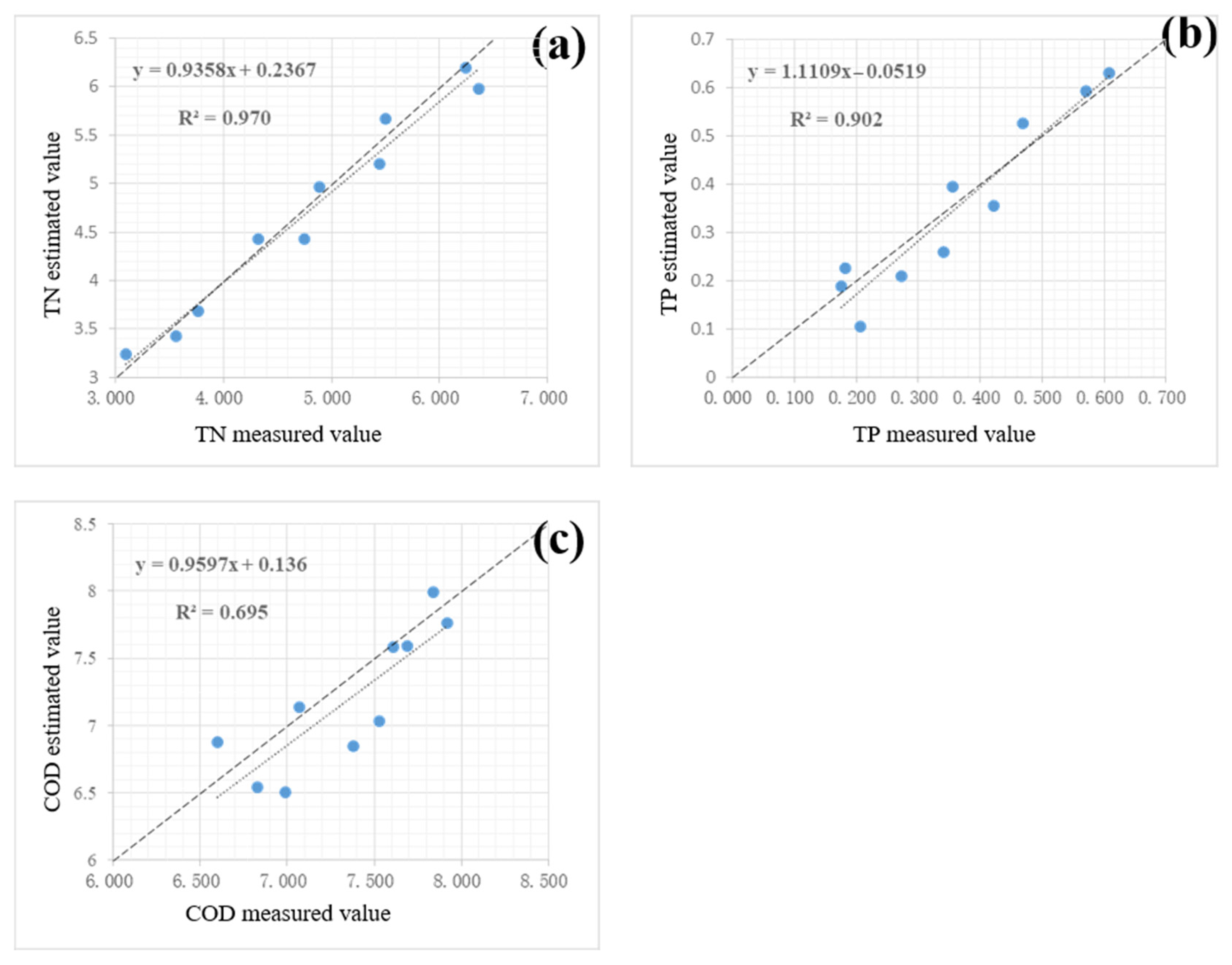
3.4. Cross-Validation for the Estimation Performance of Regression Models

Linear regressions were performed between the observed and model-estimated values of TN, TP, and COD based on the 10 validation samples. The results are presented in

Table 7. Accuracy test of water quality parameters (TN, TP, COD) estimation model.

Parameter	Estimation Model	R2	RMSE	Regression Slope
TN	ln(TN) = 1.0726 ln(NIR/R) + 5.0089	0.970	0.198	0.9358
TP	ln(TP) = 0.7235 ln(NIR/G) + 3.5681	0.902	0.057	1.1109
COD	ln(COD) = 0.2005 ln(Red_edge/G) + 0.1756	0.695	0.315	0.9597

Notes: The coefficient of determination (R²) was reported for regression models. RMSE means Root Mean Square Error.

and Figure 8. A regression slope and R² value closer to 1 indicate higher estimation accuracy. As shown in Table 7, the regression slope and coefficient of determination (R²) for the TN estimation model were 0.9358 and 0.97, respectively. For TP, the slope was 1.1109 with an R² of 0.902. The COD model yielded a slope of 0.9597 and an R² of 0.695.

As illustrated in Figure 8, the model trendlines closely align with the 1:1 reference line between observed and estimated values, suggesting that the model estimates are generally stable and in good agreement with the measured data. Overall, for the three water quality parameters examined in this study, the final model developed using the MPP approach significantly outperformed traditional satellite-based remote sensing models in terms of retrieval accuracy. This indicates the model’s strong potential for estimating the spatial distribution of water quality parameters in the Zhangshan Reservoir region.

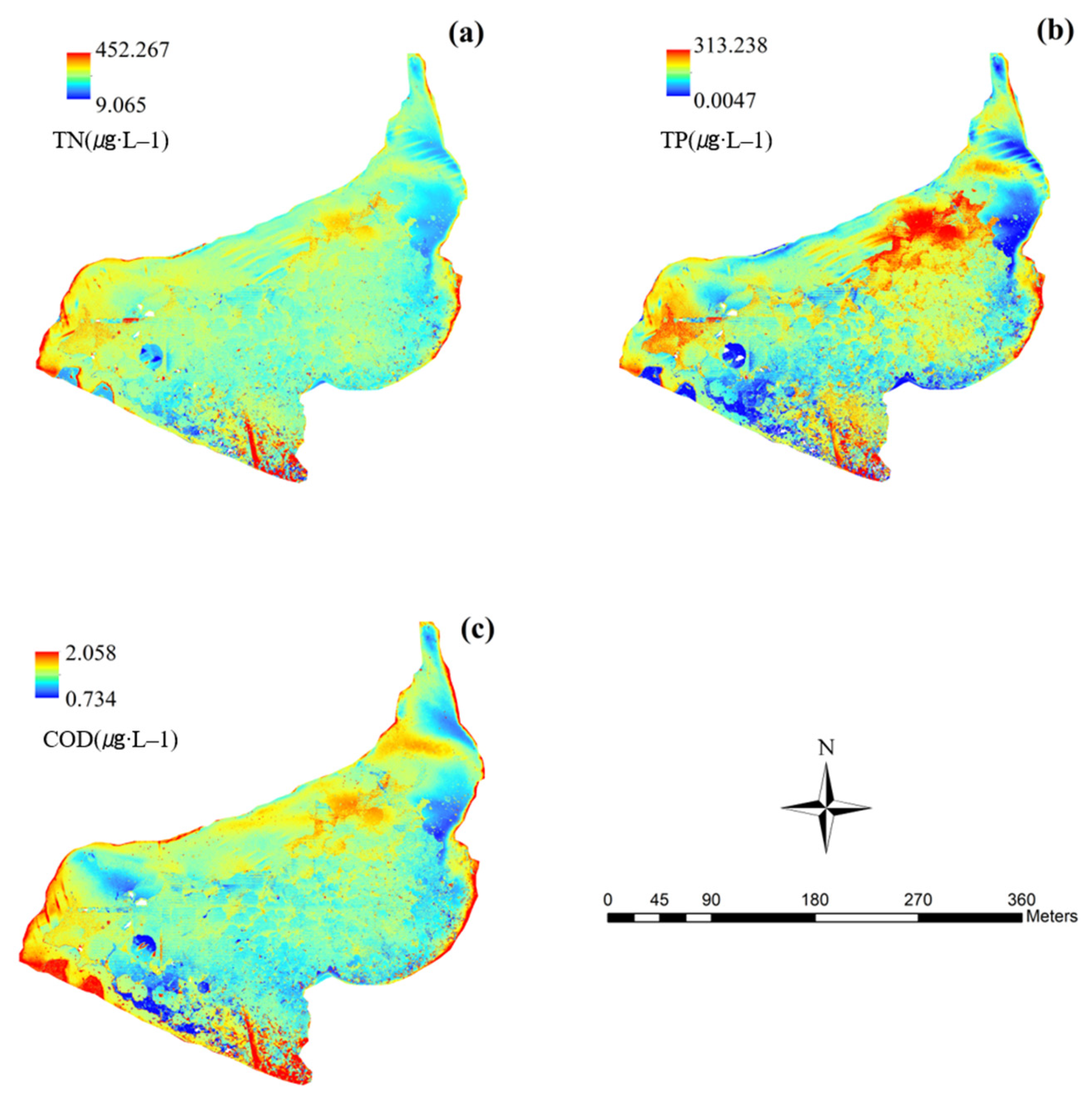
3.5. Water Quality Parameter Mapping

By comparing the regression models obtained using the WAM and MPP methods (see Table 3, Table 4 and Table 5), the MPP method yields better regression models than the WAM method. Based on Equations (2)–(4), the logarithmic transformations of the band ratios for all pixels in the UAV images are converted into the logarithmic values of water quality parameters, which are then calculated to exponential values for water quality parameter mapping.

Figure 9 displays the concentration maps of water quality parameters for Zhangshan Reservoir on 23 October 2019. Figure 9a–c were generated based on the exponential values from Equations (2)–(4). The results in Figure 9 show that low concentrations of total nitrogen, total phosphorus, and chemical oxygen demand are primarily distributed in the northeastern and southern parts of the reservoir, near the dam, and also close to sampling points E and F (see Figure 6). High concentrations of total nitrogen and total phosphorus are mainly found along the reservoir’s shore and in the northern region near the bend. Compared with the actual field conditions, these areas have sediment accumulation, are prone to ship grounding, and have some algae growth, with the water color appearing dark green.

From Figure 9, it can be seen that the highest concentration values are generally found at the edges between water and land or near the bend in the northern part. The predicted values roughly match the actual situation, and areas with high total nitrogen concentrations also show high total phosphorus concentrations and high chemical oxygen demand. According to the Carlson Trophic State Index (TSI), this study demonstrates that the nutrient status of Zhangshan Reservoir is eutrophic.

4. Discussion

4.1. Performance Comparison of WAM and MPP Algorithms

To assess the effectiveness of different spectral inversion strategies, we compared the performance of the WAM and the MPP for retrieving water quality parameters from UAV multispectral imagery. The MPP algorithm is one of the methods used to derive optimal regression equations from UAV imagery for retrieving water quality parameters. Su and Chou [40] conducted a comparative study on the performance of two pixel-based inversion approaches—WAM (Window Averaging Method, 99 × 99 pixel window) and MPP (Matched Pixel Pairing, 5 × 5 pixel window)—for estimating Chl-a, TP, and SD in the Taihu Reservoir, located in Kinmen, Taiwan Province of China [30]. Their results showed that WAM achieved a maximum coefficient of determination (R²) of 0.59 for Chl-a and 0.487 for TP. However, its performance for SD was suboptimal, with an anomalous positive correlation and a low R² of only 0.198. In contrast, MPP significantly improved inversion accuracy, with R² values reaching 0.84 for Chl-a and 0.76 for TP. Furthermore, the SD model under MPP demonstrated more physically consistent behavior, as the NIR/blue band ratio showed higher explanatory power.

These findings underscore the superior performance of MPP in small-scale reservoir environments due to its ability to achieve pixel-level alignment. This conclusion aligns with our current study, where the pixel-based MPP approach consistently outperformed the WAM method in establishing regression relationships between spectral indices and water quality parameters. Specifically, the MPP model exhibited an almost perfect predictive capability for ln(TN), with a Pearson correlation coefficient of 1.000 and R² = 1.000, whereas the best-performing WAM configuration (19 × 19 window) yielded a slightly lower R² of 0.995 (see Table 3, Table 4 and Table 5). This improvement stems from MPP’s pixel-level optimization, which effectively avoids the mixed-pixel effect commonly encountered in larger window settings of WAM. Our observations confirm that mixed pixels dilute water quality-related reflectance signals, thereby compromising model accuracy.

At present, our study has only achieved a snapshot mapping of water quality parameters for a single time period. However, effective reservoir management and sustainable water resource planning require long-term, continuous monitoring. Thus, it remains essential to identify suitable methods for producing time-series maps of water quality. In cases where a 5 × 5 window fails to yield an acceptable regression model using MPP, expanding the pixel window may be a viable strategy. Nevertheless, larger windows demand increased computational resources and carry a higher risk of model overfitting. To address these challenges, Huang, et al. [41] proposed an optimized version of MPP, termed OPT-MPP, which mitigates the computational complexity and overfitting issues associated with traditional MPP. Their results indicated that while traditional MPP achieved R² values of 0.72–0.75 for suspended solids and turbidity, it required substantial computational power. In contrast, OPT-MPP improved model performance by using a refined 3 × 3 pixel window and introducing error weighting. As a result, R² values increased to 0.787 for suspended solids and 0.804 for turbidity, while the overall model error was reduced to 0.13–0.15. These results demonstrate that OPT-MPP maintains high prediction accuracy while significantly enhancing algorithmic efficiency.

In addition, Machine learning (ML) demonstrates predictive capabilities for new data patterns, establishing its efficacy as a real-time water quality monitoring tool [42]. Parra et al. developed a low-cost RGB optical sensor combined with various machine learning algorithms—such as Gaussian Process Regression and k-Nearest Neighbors (KNN)—to perform both quantitative and classification analysis of water turbidity [43]. Similarly, Saavedra-Ruiz and Resto-Irizarry achieved high-precision water quality monitoring by integrating multiple optical sensors with machine learning techniques [42]. In their analysis of prevalent parameters in water quality research, Paepae et al. identified four principal ML algorithms: Neural Networks (NNs), Random Forest (RF), Multiple Linear Regression (MLR), and Support Vector Machines (SVMs) [44].Compared with machine learning models, the MPP algorithm offers superior spatial alignment and interpretability in small-scale water quality assessments. However, its sensitivity to noise and limited generalization capability restrict its applicability across different sites and conditions. Given the limited number of in situ samples collected from the Zhangshan Reservoir, the MPP method was adopted to maximize the use of spatially explicit information from UAV imagery. Compared to machine learning models, MPP is more suitable for small-scale studies with sparse samples due to its lower data requirements and better spatial alignment [31].

4.2. Sensitivity of Water Quality Parameters to Spectral Indices

The retrieval of TN from remote sensing imagery is typically based on empirical methods. Numerous studies have demonstrated a strong correlation between the spectral information of image pixels and TN concentrations, making it feasible to estimate TN levels from remote sensing data. Among the three water quality parameters analyzed, TN exhibited the strongest and most consistent correlation with spectral indices, particularly with ln(NIR/R). This indicates a high sensitivity of nitrogen-containing compounds to near-infrared reflectance. One possible explanation is that TN is commonly associated with both dissolved and particulate organic matter, which strongly influences surface reflectance. This relationship enables more stable and reliable spectral detection, especially in small and optically complex reservoir environments (Table 5 and Table 7). Previous studies support this finding. For example, a Landsat 8-based analysis of the Pearl River Delta achieved an R² of 0.61 for TN prediction [45]. Similarly, a UAV-based hyperspectral study in the river network of Suzhou reported a mean absolute percentage error (MAPE) below 5%, demonstrating high prediction accuracy [46]. These results confirm the feasibility of remotely sensing TN with relatively high precision.

In contrast, TP showed only moderate correlations with spectral indices, with lower R² values than TN but still within an acceptable predictive range. The weaker spectral sensitivity of TP may stem from the optical characteristics of phosphorus compounds, particularly those bound to particles, which exhibit relatively low absorption in the visible and NIR wavelengths. Furthermore, the spatial distribution of TP in surface water tends to be more heterogeneous, reducing its detectability using passive remote sensing techniques. Similar findings have been reported in previous research. For instance, a Sentinel-2-based study in Zimbabwe achieved an R² of 0.63 for TP prediction [47], while multispectral satellite data combined with regional multivariate models yielded relatively high TP estimation accuracy in Chinese lakes [48]. Nevertheless, the inherent variability and weak optical response of TP remain significant limiting factors for its remote sensing retrieval.

COD showed the weakest correlation with spectral indices across both the MPP and WAM approaches in our study (Table 5 and Table 7). This is likely due to the chemically diverse and heterogeneous nature of COD, which encompasses a wide array of oxidizable organic substances, many of which do not contribute consistently to surface reflectance. Additionally, spectral signals related to COD are often distorted by optical interference from suspended sediments, algal pigments, and colored dissolved organic matter (CDOM), especially in turbid or biologically active waters. Notably, the WAM-based model revealed a negative correlation between ln(NIR/R) and ln(COD), which contradicts the commonly reported positive trend in eutrophic waters [49]. This discrepancy may be attributed to bottom reflectance and mixed-pixel effects, particularly in shallow or highly transparent water bodies. Previous studies have further highlighted the challenges in modeling COD. For example, a UAV-based multispectral study in coastal aquaculture ponds achieved an R² > 0.8 for COD [32], while research in the Xiong’an New Area reported R² values ranging from 0.78 to 0.89 [50]. However, these studies also noted that key absorption features for COD lie in the ultraviolet spectrum, which is not captured by most current optical sensors, thereby limiting detection capability.

In summary, TN is typically the most reliably predicted water quality parameter via remote sensing, followed by TP, with COD posing the greatest modeling challenges. These differences primarily arise from each parameter’s spectral responsiveness, spatial distribution characteristics, and interaction with other optically active substances. Therefore, the selection of appropriate sensors and modeling approaches should be tailored to the specific spectral and spatial behavior of each parameter in order to enhance prediction accuracy and support effective water quality monitoring.

4.3. Application Value and Limitations

The study by Su and Chou [40] represents an early and foundational example of using UAV-based multispectral imagery to retrieve Chl-a and TP concentrations in the Taihu Reservoir. Their work successfully demonstrated the potential of UAVs as viable alternatives to traditional satellite platforms for monitoring small-scale reservoirs. Building upon this, our study integrated UAV-derived spectral data with in-situ water sampling to generate spatial distribution maps of key water quality parameters. Notably, areas of elevated TN, TP, and COD were primarily concentrated along the littoral zones and reservoir bends—regions typically characterized by sediment accumulation, reduced water flow, and algal aggregation. These patterns indicate localized nutrient buildup and the presence of eutrophication hotspots (Figure 9).

Based on the Carlson Trophic State Index [51] the Zhangshan Reservoir was classified as eutrophic during the sampling period, consistent with field observations of dark green, algae-rich waters. The spatial insights derived from this study can serve as a scientific basis for targeted interventions, such as ecological restoration and water quality management strategies. Wang et al. [52] advocated for the integration of UAV multispectral data with satellite-based remote sensing platforms such as MODIS to achieve long-term, continuous monitoring of reservoir water quality, thereby compensating for the limitations of single-platform approaches. While the MPP algorithm in our study demonstrated strong predictive performance, its accuracy is highly sensitive to the spatial alignment between sampling points and image pixels. Geolocation errors can significantly reduce model reliability. Prior et al. [53] highlighted that the high spatial resolution of UAV imagery poses challenges in matching pixels to field samples, necessitating the use of ground control points (GCPs) and differential GNSS systems to improve geometric correction accuracy. In our case, handheld GPS units were used to precisely georeference sample sites, ensuring consistency between field locations and UAV pixel scales (Table 1).

However, the generalizability of our model is constrained by a limited sample size [18]. Although the study collected a total of 60 water samples across six spatially distributed sites, the relatively small number of distinct sampling locations may constrain the generalizability of the regression models. While the achieved sampling density (17.65 points/km²) exceeds typical values reported in the literature for reservoir monitoring, the model’s spatial robustness across heterogeneous or temporally dynamic conditions remains uncertain.

Moreover, a notable limitation of this study is that both UAV imaging and in-situ water sampling were conducted on a single day. While this design ensured strict temporal consistency—an essential condition for establishing accurate regression relationships—it also means that the developed models reflect only a snapshot of water quality conditions under specific meteorological and hydrological settings. Reservoir water quality can exhibit temporal variability due to rainfall events, seasonal changes, or biological processes. Consequently, the temporal generalizability of the models developed in this study may be limited.

Furthermore, we do not claim that the regression models developed in this study are directly transferable to other reservoir environments, as they are inherently influenced by local optical properties, water composition, and environmental conditions. However, the methodology—particularly the integration of UAV multispectral data with the Matched Pixel Pairing (MPP) algorithm—demonstrates clear applicability for similar studies in small- to medium-sized water bodies with limited field sampling capacity. This framework provides a practical solution for achieving fine-scale water quality estimation when extensive in-situ measurements are not feasible, and may serve as a baseline for localized model development in other study areas. Future studies should incorporate multi-temporal sampling and UAV data acquisition to improve model robustness and better account for temporal fluctuations in water quality [54]. Additionally, there is a growing need to establish industry standards for UAV-based water quality monitoring, including sensor calibration, flight parameters (e.g., altitude, image overlap), and standardized data processing protocols [55].

5. Conclusions

In this study, 60 surface water samples were collected from six sites within Zhangshan Reservoir, a small reservoir in Chuzhou, Anhui, China, to analyze spatial variation in water quality. The results showed that TN concentrations were generally high across all sites; COD and TP levels also varied spatially, indicating localized pollution. Multispectral UAV imagery combined with two modeling approaches—WAM and MPP—was used to estimate water quality parameters. The WAM method performed well for TN but poorly for TP and COD, while the MPP approach achieved high accuracy for all three parameters, with R² values of 0.970, 0.902, and 0.695 for TN, TP, and COD, respectively. These results highlight the advantages of UAV-based fine-scale monitoring in small water bodies, where traditional remote sensing may struggle due to pixel mixing and resolution constraints.

From a management perspective, the high TN levels point to potential nitrogen input sources that warrant targeted control, especially in the northwest areas of the reservoir. Accurate spatial mapping of TN, TP, and COD can support early pollution warnings and inform site-specific intervention strategies. However, this study has limitations. The sampling was conducted on a single day, and the sample size was relatively small. In addition, only surface water was assessed, and seasonal or depth-related variations were not captured. These factors may constrain the generalizability of the models.

Future work should incorporate multi-seasonal, multi-depth sampling and explore the integration of additional spectral features or machine learning techniques to improve the model transferability. Furthermore, expanding the dataset would help validate the robustness of regression models and support the development of operational water quality monitoring systems using UAV remote sensing.

References

1. Sun, B.; Zhang, L.; Yang, L.; Zhang, F.; Norse, D.; Zhu, Z. Agricultural non-point source pollution in China: Causes and mitigation measures. Ambio 2012, 41, 370–379. [Google Scholar] [CrossRef] [PubMed]
2. Lu, Y.; Wang, C.; Yang, R.; Sun, M.; Zhang, L.; Zhang, Y.; Li, X. Research on the progress of agricultural non-point source pollution management in China: A review. Sustainability 2023, 15, 13308. [Google Scholar] [CrossRef]
3. Lo, Y.; Fu, L.; Lu, T.; Huang, H.; Kong, L.; Xu, Y.; Zhang, C. Medium-sized lake water quality parameters retrieval using multispectral uav image and machine learning algorithms: A case study of the yuandang lake, China. Drones 2023, 7, 244. [Google Scholar] [CrossRef]
4. Kijowska-Strugala, M.; Wiejaczka, L.; Kozlowski, R. Influence of reservoirs on the concentration of nutrients in the water of mountain rivers. Ecol. Chem. Eng. 2016, 23, 413. [Google Scholar] [CrossRef]
5. Yang, X.; Lu, X. Drastic change in China’s lakes and reservoirs over the past decades. Sci. Rep. 2014, 4, 6041. [Google Scholar] [CrossRef]
6. Sani, S.A. Drawbacks of Traditional Environmental Monitoring Systems. TMP Univers. J. Res. Rev. Arch. 2023, 2, srep06041. [Google Scholar] [CrossRef]
7. Bourouhou, I.; Salmoun, F. Sea water quality monitoring using remote sensing techniques: A case study in Tangier-Ksar Sghir coastline. Environ. Monit. Assess. 2021, 193, 557. [Google Scholar] [CrossRef]
8. Tv, R. Remote sensing applications in water resources. J. Indian Inst. Sci. 2013, 93, 163–188. [Google Scholar]
9. Wasehun, E.T.; Hashemi Beni, L.; Di Vittorio, C.A. UAV and satellite remote sensing for inland water quality assessments: A literature review. Environ. Monit. Assess. 2024, 196, 277. [Google Scholar] [CrossRef]
10. Raghul, M.; Porchelvan, P. A Critical Review of Remote Sensing Methods for Inland Water Quality Monitoring: Progress, Limitations, and Future Perspectives. Water Air Soil Pollut. 2024, 235, 159. [Google Scholar] [CrossRef]
11. Wong, M.S.; Zhu, X.; Abbas, S.; Kwok, C.Y.T.; Wang, M. Optical remote sensing. In Urban Informatics; Springer: Singapore, 2021; pp. 315–344. [Google Scholar]
12. Dörnhöfer, K.; Oppelt, N. Remote sensing for lake research and monitoring–Recent advances. Ecol. Indic. 2016, 64, 105–122. [Google Scholar] [CrossRef]
13. Lim, J.; Choi, M. Assessment of water quality based on Landsat 8 operational land imager associated with human activities in Korea. Environ. Monit. Assess. 2015, 187, 384. [Google Scholar] [CrossRef]
14. Garg, V.; Aggarwal, S.P.; Chauhan, P. Changes in turbidity along Ganga River using Sentinel-2 satellite data during lockdown associated with COVID-19. Geomat. Nat. Hazards Risk 2020, 11, 1175–1195. [Google Scholar] [CrossRef]
15. Baban, S.M.J. Detecting water quality parameters in the Norfolk Broads, UK, using Landsat imagery. Int. J. Remote Sens. 1993, 14, 1247–1267. [Google Scholar] [CrossRef]
16. Kulkarni, A. Water quality retrieval from Landsat TM imagery. Procedia Comput. Sci. 2011, 6, 475–480. [Google Scholar] [CrossRef]
17. Bonansea, M.; Ledesma, C.; Rodríguez, C.; Pinotti, L.; Antunes, M.H. Effects of atmospheric correction of Landsat imagery on lake water clarity assessment. Adv. Space Res. 2015, 56, 2345–2355. [Google Scholar] [CrossRef]
18. Chen, L.; Tan, C.-H.; Kao, S.-J.; Wang, T.-S. Improvement of remote monitoring on water quality in a subtropical reservoir by incorporating grammatical evolution with parallel genetic algorithms into satellite imagery. Water Res. 2008, 42, 296–306. [Google Scholar] [CrossRef]
19. Gholizadeh, M.H.; Melesse, A.M.; Reddi, L. A Comprehensive Review on Water Quality Parameters Estimation Using Remote Sensing Techniques. Sensors 2016, 16, 1298. [Google Scholar] [CrossRef]
20. Song, K.; Li, L.; Li, S.; Tedesco, L.; Hall, B.; Li, L. Hyperspectral Remote Sensing of Total Phosphorus (TP) in Three Central Indiana Water Supply Reservoirs. Water Air Soil Pollut. 2012, 223, 1481–1502. [Google Scholar] [CrossRef]
21. Singh, Y.; Walingo, T. Smart Water Quality Monitoring with IoT Wireless Sensor Networks. Sensors 2024, 24, 2871. [Google Scholar] [CrossRef]
22. Reiners, P.; Sobrino, J.; Kuenzer, C. Satellite-Derived Land Surface Temperature Dynamics in the Context of Global Change—A Review. Remote Sens. 2023, 15, 1857. [Google Scholar] [CrossRef]
23. Mansaray, A.S.; Dzialowski, A.R.; Martin, M.E.; Wagner, K.L.; Gholizadeh, H.; Stoodley, S.H. Comparing PlanetScope to Landsat-8 and Sentinel-2 for Sensing Water Quality in Reservoirs in Agricultural Watersheds. Remote Sens. 2021, 13, 1847. [Google Scholar] [CrossRef]
24. Cheng, C.; Zhang, F.; Shi, J.; Kung, H.T. What is the relationship between land use and surface water quality? A review and prospects from remote sensing perspective. Environ. Sci. Pollut. Res. Int. 2022, 29, 56887–56907. [Google Scholar] [CrossRef]
25. Yang, H.; Kong, J.; Hu, H.; Du, Y.; Gao, M.; Chen, F. A Review of Remote Sensing for Water Quality Retrieval: Progress and Challenges. Remote Sens. 2022, 14, 1770. [Google Scholar] [CrossRef]
26. Mishra, V.; Avtar, R.; Prathiba, A.P.; Mishra, P.K.; Tiwari, A.; Sharma, S.K.; Singh, C.H.; Chandra Yadav, B.; Jain, K. Uncrewed aerial systems in water resource management and monitoring: A review of sensors, applications, software, and issues. Adv. Civ. Eng. 2023, 2023, 3544724. [Google Scholar] [CrossRef]
27. Cillero Castro, C.; Domínguez Gómez, J.A.; Delgado Martín, J.; Hinojo Sánchez, B.A.; Cereijo Arango, J.L.; Cheda Tuya, F.A.; Díaz-Varela, R. An UAV and Satellite Multispectral Data Approach to Monitor Water Quality in Small Reservoirs. Remote Sens. 2020, 12, 1514. [Google Scholar] [CrossRef]
28. Román, A.; Tovar-Sánchez, A.; Gauci, A.; Deidun, A.; Caballero, I.; Colica, E.; D’Amico, S.; Navarro, G. Water-Quality Monitoring with a UAV-Mounted Multispectral Camera in Coastal Waters. Remote Sens. 2023, 15, 237. [Google Scholar] [CrossRef]
29. Liu, X.; Wang, Y.; Chen, T.; Gu, X.; Zhang, L.; Li, X.; Tang, R.; He, Y.; Chen, G.; Zhang, B. Monitoring water quality parameters of freshwater aquaculture ponds using UAV-based multispectral images. Ecol. Indic. 2024, 167, 112644. [Google Scholar] [CrossRef]
30. TungChing, S. A study of a matching pixel by pixel (MPP) algorithm to establish an empirical model of water quality mapping, as based on unmanned aerial vehicle (UAV) images. Int. J. Appl. Earth Obs. Geoinf. 2017, 58, 213–224. [Google Scholar] [CrossRef]
31. Ying, H.; Xia, K.; Huang, X.; Feng, H.; Yang, Y.; Du, X.; Huang, L. Evaluation of water quality based on UAV images and the IMP-MPP algorithm. Ecol. Inform. 2021, 61, 101239. [Google Scholar] [CrossRef]
32. Zhang, Y.; Jing, W.; Deng, Y.; Zhou, W.; Yang, J.; Li, Y.; Cai, Y.; Hu, Y.; Peng, X.; Lan, W. Water quality parameters retrieval of coastal mariculture ponds based on UAV multispectral remote sensing. Front. Environ. Sci. 2023, 11, 1079397. [Google Scholar] [CrossRef]
33. Xiao, Y.; Guo, Y.; Yin, G.; Zhang, X.; Shi, Y.; Hao, F.; Fu, Y. UAV Multispectral Image-Based Urban River Water Quality Monitoring Using Stacked Ensemble Machine Learning Algorithms—A Case Study of the Zhanghe River, China. Remote Sens. 2022, 14, 3272. [Google Scholar] [CrossRef]
34. Chen, B.; Mu, X.; Chen, P.; Wang, B.; Choi, J.; Park, H.; Xu, S.; Wu, Y.; Yang, H. Machine learning-based inversion of water quality parameters in typical reach of the urban river by UAV multispectral data. Ecol. Indic. 2021, 133, 108434. [Google Scholar] [CrossRef]
35. Bureau, A.P.H. Real-Time Water Information of Zhangshan Reservoir. Available online: http://yc.wswj.net/ahsxx/LOL/?refer=upl&to=public_public (accessed on 23 October 2019).
36. Wang, Z.; Hong, J.; Du, G. Use of satellite imagery to assess the trophic state of Miyun Reservoir, Beijing, China. Environ. Pollut. 2008, 155, 13–19. [Google Scholar]
37. Michaelsen, E.; Meidow, J. Stochastic reasoning for structural pattern recognition: An example from image-based UAV navigation. Pattern Recognit. 2014, 47, 2732–2744. [Google Scholar] [CrossRef]
38. Zaman, B.; Jensen, A.; Clemens, S.R.; McKee, M. Retrieval of spectral reflectance of high resolution multispectral imagery acquired with an autonomous unmanned aerial vehicle. Photogramm. Eng. Remote Sens. 2014, 80, 1139–1150. [Google Scholar]
39. Sriwongsitanon, N.; Surakit, K.; Thianpopirug, S. Influence of atmospheric correction and number of sampling points on the accuracy of water clarity assessment using remote sensing application. J. Hydrol. 2011, 401, 203–220. [Google Scholar] [CrossRef]
40. Su, T.-C.; Chou, H.-T. Application of multispectral sensors carried on unmanned aerial vehicle (UAV) to trophic state mapping of small reservoirs: A case study of Tain-Pu reservoir in Kinmen, Taiwan. Remote Sens. 2015, 7, 10078–10097. [Google Scholar] [CrossRef]
41. Huang, X.-X.; Ying, H.-T.; Xia, K.; Feng, H.-L.; Yang, Y.-H.; Du, X.-C. Inversion of water quality parameters based on UAV multispectral images and the OPT-MPP algorithm. Huan Jing Ke Xue=Huanjing Kexue 2020, 41, 3591–3600. [Google Scholar]
42. Saavedra-Ruiz, A.; Resto-Irizarry, P.J. A Portable UV-LED/RGB Sensor for Real-Time Bacteriological Water Quality Monitoring Using ML-Based MPN Estimation. Biosensors 2025, 15, 284. [Google Scholar] [CrossRef]
43. Parra, L.; Ahmad, A.; Sendra, S.; Lloret, J.; Lorenz, P. Combination of Machine Learning and RGB Sensors to Quantify and Classify Water Turbidity. Chemosensors 2024, 12, 34. [Google Scholar] [CrossRef]
44. Paepae, T.; Bokoro, P.N.; Kyamakya, K. From Fully Physical to Virtual Sensing for Water Quality Assessment: A Comprehensive Review of the Relevant State-of-the-Art. Sensors 2021, 21, 6971. [Google Scholar] [CrossRef]
45. Guo, Y.; Deng, R.; Li, J.; Hua, Z.; Wang, J.; Zhang, R.; Liang, Y.; Tang, Y. Remote Sensing Retrieval of Total Nitrogen in the Pearl River Delta Based on Landsat8. Remote Sens. 2022, 14, 3710. [Google Scholar] [CrossRef]
46. Zhang, D.; Zeng, S.; He, W. Selection and Quantification of Best Water Quality Indicators Using UAV-Mounted Hyperspectral Data: A Case Focusing on a Local River Network in Suzhou City, China. Sustainability 2022, 14, 16226. [Google Scholar] [CrossRef]
47. Muhoyi, H.; Gumindoga, W.; Mhizha, A.; Misi, S.N.; Nondo, N. Water quality monitoring using remote sensing, Lower Manyame Sub-catchment, Zimbabwe. Water Pract. Technol. 2022, 17, 1347–1357. [Google Scholar] [CrossRef]
48. Gao, Y.; Gao, J.; Yin, H.; Liu, C.; Xia, T.; Wang, J.; Huang, Q. Remote sensing estimation of the total phosphorus concentration in a large lake using band combinations and regional multivariate statistical modeling techniques. J. Environ. Manag. 2015, 151, 33–43. [Google Scholar] [CrossRef]
49. Komas, J.M. Measuring Optical Water Quality Parameters Using an Unmanned Aerial Vehicle (UAV)-Based Multispectral Sensor, Lake Bloomington and Evergreen Lake; Illinois State University: Normal, IL, USA, 2022. [Google Scholar]
50. Yang, Y.; Zhang, D.; Li, X.; Wang, D.; Yang, C.; Wang, J. Winter Water Quality Modeling in Xiong’an New Area Supported by Hyperspectral Observation. Sensors 2023, 23, 4089. [Google Scholar] [CrossRef]
51. Carlson, R.E. A trophic state index for lakes 1. Limnol. Oceanogr. 1977, 22, 361–369. [Google Scholar] [CrossRef]
52. Wang, S.; Li, J.; Zhang, B.; Lee, Z.; Spyrakos, E.; Feng, L.; Liu, C.; Zhao, H.; Wu, Y.; Zhu, L. Changes of water clarity in large lakes and reservoirs across China observed from long-term MODIS. Remote Sens. Environ. 2020, 247, 111949. [Google Scholar] [CrossRef]
53. Prior, E.M.; O’Donnell, F.C.; Brodbeck, C.; Runion, G.B.; Shepherd, S.L. Investigating small unoccupied aerial systems (sUAS) multispectral imagery for total suspended solids and turbidity monitoring in small streams. Int. J. Remote Sens. 2021, 42, 39–64. [Google Scholar] [CrossRef]
54. Feng, L.; Hu, C.; Han, X.; Chen, X.; Qi, L. Long-Term Distribution Patterns of Chlorophyll-a Concentration in China’s Largest Freshwater Lake: MERIS Full-Resolution Observations with a Practical Approach. Remote Sens. 2015, 7, 275–299. [Google Scholar] [CrossRef]
55. Gai, Y.; Yu, D.; Zhou, Y.; Yang, L.; Chen, C.; Chen, J. An improved model for chlorophyll-a concentration retrieval in coastal waters based on UAV-Borne hyperspectral imagery: A case study in Qingdao, China. Water 2020, 12, 2769. [Google Scholar] [CrossRef]
Figure 1. Location of study area: (a) Chuzhou City, Anhui Province, China. (b) the position of six water sample collection points of Zhangshan reservoir. Points A–F are the sampling points, evenly distributed according to the shape of the reservoir water surface. Our sampling sequence is from A to F in sequence.
Water 17 01566 g001
Figure 2. UAV imagery system: (a) Sequoia multispectral red-edge sensor; (b) Multi-rotor M600Pro.
Water 17 01566 g002
Figure 3. (a) Proposed locations and style of GCPs and checking points; (b) Flight path and empty three encryption processing aerial triangulation (780 schemed camera stations: red is the aerial triangulation processing part).
Water 17 01566 g003
Figure 4. Pix4Dmapper processing workflow (blue: flight direction; red: image acquisition points).
Water 17 01566 g004
Figure 5. Image overlap.
Water 17 01566 g005
Figure 6. Final mosaicked images for each spectral band (a) Green band reflection, (b) Red band reflection, (c) Red_edge band reflection, (d) NIR band reflection.
Water 17 01566 g006
Figure 7. Flowchart of applying UAV multispectral imagery coupled with measurement in situ to water quality parameters mapping.
Water 17 01566 g007
Figure 8. Fitting maps of estimated values and measured values of water quality parameters: (a) TN fitting map; (b) TP fitting map; (c) COD fitting map.
Water 17 01566 g008
Figure 9. Concentration maps of water quality parameters of Zhangshan reservoir on 23 October 2019: (a) TN concentration map; (b) TP concentration map; (c) COD concentration map.
Water 17 01566 g009