Article

Effects of Green Infrastructure Practices on Runoff and Water Quality in the Arroyo Colorado Watershed, Texas

Department of Environmental Engineering, Texas A&M University—Kingsville, MSC 213, 925 W. Avenue B, Kingsville, TX 78363, USA
*
Author to whom correspondence should be addressed.
Water 2025, 17(11), 1565; https://doi.org/10.3390/w17111565
Submission received: 22 March 2025 / Revised: 12 May 2025 / Accepted: 19 May 2025 / Published: 22 May 2025
(This article belongs to the Special Issue Urban Stormwater Control, Utilization, and Treatment)

Abstract

:
Continuous use of agricultural chemicals and fertilizers, sporadic sewer overflow events, and an increase in urbanization have led to significant nutrient/pollutant loadings into the semi-arid Arroyo Colorado River basin, which is located in South Texas, U.S. Priority nutrients that require reduction include phosphorus and nitrogen and to mitigate issues of low dissolved oxygen, in some of its river segments. Consequently, the river’s potential to support aquatic life has been significantly reduced, thus highlighting the need for restoration. To achieve this restoration, a watershed protection plan was developed, comprising several preventive mitigation measures, including installing green infrastructure (GI) practices. However, for effective reduction of excessive nutrient loadings, there is a need to study the effects of different combinations of GI practices under current and future land use scenarios to guide decisions in implementing the cost-effective infrastructure while considering factors such as the existing drainage system, topography, land use, and streamflow. Therefore, this study coupled the Soil and Water Assessment Tool (SWAT) model with the System for Urban Stormwater Treatment and Analysis Integration (SUSTAIN) model to determine the effects of different combinations of GI practices on the reduction of nitrogen and phosphorus under changing land use conditions in three selected Arroyo Colorado subwatersheds. Two land use maps from the U.S. Geological Survey (USGS) Forecasting Scenarios of land use (FORE-SCE) model for 2050, namely, A1B and B1, were implemented in the coupled SWAT-SUSTAIN model in this study, where the urban area is projected to increase by 6% and 4%, respectively, with respect to the 2018 land use scenario. As expected, runoff, phosphorus, and nitrogen slightly increased with imperviousness. The modeling results showed that implementing either vegetated swales or wet ponds reduces flow and nutrients to meet the Total Maximum Daily Loads (TMDLs) targets, which cost about USD 1.5 million under current land use (2018). Under the 2050 future projected land use changes (A1B scenario), the cost-effective GI practice was implemented in vegetated swales at USD 1.5 million. In contrast, bioretention cells occupied the least land area to achieve the TMDL targets at USD 2 million. Under the B1 scenario of 2050 projected land use, porous pavements were most cost effective at USD 1.5 million to meet the TMDL requirements. This research emphasizes the need for collaboration between stakeholders at the watershed and farm levels to achieve TMDL targets. This study informs decision-makers, city planners, watershed managers, and other stakeholders involved in restoration efforts in the Arroyo Colorado basin.

1. Introduction

Increased urbanization, coupled with intense agricultural production involving the application of fertilizers and pesticides, significantly contributes to the declining water quality of the watersheds in the United States [1]. This, coupled with the increased magnitude and intensity of extreme events in recent decades, has resulted in increased sewer overflow events and the transport of pollutants into the receiving water bodies, causing their contamination and impairment [2]. Urbanization increases the impervious areas, thus changing the hydrologic regime of a watershed, resulting in higher volumes of runoff, reduced infiltration rates, higher peak flows, and washing-off of large amounts of pollutants into receiving water bodies [3,4]. With urbanization and population growth, the impervious areas increase, leading to increased runoff peaks and the pollution of receiving water bodies.
Pollution of receiving water occurs due to many factors, one of which is the accumulation of excessive nutrients. Excessive amounts of nutrients such as phosphorus and nitrogen can lead to eutrophication, which can reduce the amounts of dissolved oxygen in a river, causing it to be classified as impaired [5,6]. For example, the Arroyo Colorado River in the semi-arid region of South Texas is one of the rivers listed as an impaired water body [7]. Recent studies highlight the need to implement pollution mitigation strategies to address the issue of impairment [8]. In addition, continuous development in the Arroyo Colorado Watershed has resulted in a shift from permeable areas to impermeable surfaces to accommodate growth and population increase. This conversion increases urban pollutants such as nitrogen, phosphorus, zinc, copper, and lead, which result from infrastructural developments due to population growth [5]. The U.S. EPA established the Clean Water Act section 303(d), which requires the states to establish Total Maximum Loads (TMDLs) for any water body within their jurisdiction that is impaired [9]. Under this act, each state is charged with the management of both point and non-point pollution sources using load allocation to ensure that the water bodies achieve the regulatory water quality standards. To achieve this, land management can be conducted in various ways, one of which is categorizing a watershed into land use types and managing the pollution sources based on land use types.
Management of point and non-point source pollution in watersheds can also be conducted through the use of green infrastructure (GI), which refers to the Best Management Practices (BMPs) and the Low Impact Development (LID) structures, both aimed at restoring the natural hydrological regime of watersheds [10]. GI practices combine the retention, detention, and infiltration processes to decrease runoff volumes and rates, increase storage, promote infiltration, delay runoff peaks, and control pollutant movement [11,12]. BMPs refer to large-scale GI structures such as wetland basins, detention basins, and retention ponds, usually installed at the drainage basin outlet to capture and treat stormwater runoff [12]. LIDs refer to small-scale GI practices such as vegetated swales, rain gardens, and porous pavements, which are designed to capture and treat runoff at the source instead of conveying it to an outlet [13].
Various BMPs have different effectiveness for removing pollutants from non-point sources in watersheds. For example, agricultural BMPs such as nutrient management, crop rotation, erosion control, and terraces have been employed and shown varying effectiveness based on the application, pollutant type, and their application timing [14,15]. For a watershed with mixed land use (i.e., with multiple dominant land uses such as agriculture and urban), agricultural BMPs should be applied in parallel to urban BMPs. Urban BMPs can be categorized into the treat and release BMPs and infiltration BMPs, each with varying functionality [10]. Treat and release BMPs, such as wet ponds and vegetated swales, capture stormwater, treat it, and then release it back into the drainage network. Such BMPs usually have an underdrain pipe to collect all the treated stormwater for release into the drainage network. The advantage of treat and release BMPs is that the underlying soils are not considered during their construction, since enhancing infiltration is not required. The significant disadvantage, however, is that there is a need to adjust the drainage network. The drainage network may need to be adjusted since excessive amounts of water could run into the drainage network during high-intensity storms. On the other hand, infiltration BMPs such as bioretention cells and porous pavements capture stormwater, treat it, and infiltrate it into the ground surface. Therefore, such BMPs must be constructed in highly permeable soils, or an infiltration medium is required at the bottom. The advantages of infiltration BMPs are that they do not add an extra load to the drainage network and replenish groundwater. The disadvantage is that they can only be constructed on soils with high-infiltration capacity, and therefore, there is an added cost of a permeable layer at the bottom [3,10].
Several hydrologic models have been used to evaluate the effects of land management practices on pollutant removal efficiencies. For example, lumped models, such as the Nonpoint Source Pollution and Erosion Comparison Tool (N-SPECT), assume a homogenous watershed and thus model it as a single management and land cover unit. On the other hand, spatially distributed models such as the Soil and Water Assessment Tool (SWAT) model represent a watershed using spatial variability in the geospatial data by dividing the watershed into smaller units referred to as hydrological response units based on soil, land use, and slope [16,17,18,19]. In particular, the Source Loading and Management Model for Windows (WinSLAMM), developed by the U.S. Geological Survey (USGS) [20], evaluates stormwater controls using design values and actual field data in urban areas. Another model frequently used to study stormwater is the Environmental Protection Agency’s (EPA) Stormwater Management Model (SWMM), which is a dynamic rainfall–runoff model used to simulate flow and pollutants from urban watersheds [21,22]. However, these models are not adapted for agricultural watersheds and do not include cost-benefit analysis tools or components. To incorporate cost analysis, the US EPA developed the SUSTAIN model, a multiscale comprehensive watershed model that builds on ArcGIS as an add-in to simulate water quality. It carries out cost optimization for various BMP components, thus facilitating the placement of GI at multiple locations in a watershed [21,22].
The Arroyo Colorado Watershed Management Plan recommends combining GI practices to restore the river’s water quality [8]. Previous research carried out in the watershed focused on the use of agricultural BMPs for water quality improvement, such as crop rotation, irrigation scheduling, nutrient management, residue management, and terracing [15,17,23]. However, research on urban GI practices in the watershed is still limited. Additionally, the variability in watershed characteristics, such as flat topography and soils with varying infiltration capacity, influences the type of GI practices that can effectively reduce pollutants. This, coupled with limited funding to implement GI practices, requires the optimal selection and placement of GI in a watershed to minimize pollutants and cost-effectively reduce runoff [24]. Therefore, in this study, the SUSTAIN model was used to determine the cost-effective strategies for pollutant removal. Several modules exist in SUSTAIN for BMPs simulation, data management, analysis of spatial information, optimization, and network visualization [21,22]. However, it needs to be coupled to an external model through the external model simulation module. Thus, the SUSTAIN model was coupled with the SWAT model to determine the effects of green infrastructure (GI) practices on reducing runoff, phosphorus, and nitrogen in the Arroyo Colorado Watershed under current and future land use/cover changes. Therefore, the research objectives addressed in this study are to (i) estimate the optimal costs of implementing GI practices to achieve TMDL targets for total nitrogen and phosphorus in the Arroyo Colorado Watershed (ACW) under recent land use, and (ii) determine the combination of GI practices that achieves the lowest loading of nutrients to the ACW at a minimum cost under future (2050) land use projections.

2. Background and Methodology

2.1. Study Area

The Arroyo Colorado Watershed (ACW) is in the Rio Grande Valley of South Texas (Figure 1). It was selected for this study due to water quality issues and concerns in the river segments. The ACW is located on the ACR, which is 90 miles long, originating near Mission, Texas, and draining into the Lower Laguna Madre. The total drainage area of the watershed is 706 square miles (1828.53 sq. km) with an average slope of 1.5 feet per mile [8]. Three subwatersheds (Mission area, Weslaco area, and Mercedes area) were selected for this study due to relatively high percentages of urban and agricultural land uses and the availability of water quality data and monitoring stations (Figure 1).
The fractional land use composition for different land use categories was estimated in percentage by dividing the area under each land use category by the total area of each subwatershed based on the 2018 National Land Cover Dataset (NLCD) land use data [25]. Subwatershed 1 is the Mission area subwatershed, with 40.6% of the area under urban land use and 45.9% under agriculture (Table 1). Subwatershed 2 is the Weslaco area, with 23.7% and 60.7% in urban and agricultural areas, respectively. Subwatershed 3, the Mercedes area, has 15% urban and 62.9% agricultural land use (Table 1). The total area of the three subwatersheds is 163,850 acres (671.54 sq. km).

2.2. Input Data

To implement the SUSTAIN model, this study used the SWAT model to generate a time series of flow and pollutant loadings from the different subwatersheds. For the SWAT modeling, the input data and their sources are provided in Table 2.

2.3. SWAT Modeling

A SWAT 2012 model was set up and modeled as the base case scenario. SWAT is a distributed hydrological model based on ArcGIS that simulates the major hydrological components such as precipitation, runoff, wind, temperature, evapotranspiration, and percolation [16]. SWAT carries out hydrological modeling by dividing the watershed into several smaller subwatersheds and simulating each of them [16]. These subwatersheds are further subdivided into units based on land use, soil type, and slope, called Hydrologic Response Units (HRUs). Output from the SWAT model in the form of time series data for the HRUs, is required to run SUSTAIN through the incorporation of an external simulation model.
Calibration of SWAT was performed using the SWATCUP, a widely used SWAT calibration program [32]. The Sequential Uncertainty Fitting Version-2 (SUFI-2) in SWAT-CUP was used to fit model outputs to observed USGS streamflow data and measured TCEQ SWQM water quality data. The metrics used to evaluate the performance of the model include the Coefficient of Determination (R2) and Nash Sutcliffe Efficiency (NSE) [32]. The R2 represents the linear relationship between the observed and model output values. An R2 value greater than 0.6 and an NSE of more than 0.5 represent a satisfactory level of model calibration [33]. The NSE is used to assess the difference between the variance of the model and the measured data variance. An NSE value of 1 shows a perfectly calibrated model. The SWAT model was calibrated to match the variability of simulated flows to observed flows. The model was calibrated from January 2013 to December 2020. The first one-year (2012) simulations served as the model spin-up period. Based on a review of other studies and the recommendations of the SWAT-CUP manual, the following parameters (Table 3) were considered for calibration of streamflow, total nitrogen, and total phosphorus [5,15,17,32,34].

2.4. SUSTAIN Modeling

2.4.1. SUSTAIN Set up

HRU time series results from the SWAT model were used to run the SUSTAIN model (as external time series) to simulate similar flows and water quality conditions as estimated by the calibrated SWAT model with no new GI practices. Typical parameters adjusted in SUSTAIN for flow and water quality calibration (Table 4) are as follows: hydraulic conductivity, Manning’s N roughness coefficient for impervious and pervious areas, and depression storage for pervious and impervious areas [21] (Shoemaker et al., 2011). Once the SUSTAIN model was calibrated to match streamflow and water quality indicators estimated by the SWAT model, it was used for further analysis to estimate the effects of various GI practices. The GI practices selected as the focus of this research were based on previous studies [17,23] conducted in this watershed, in which it was determined that the watershed requires bioretention cells, porous pavements, vegetated swales, and wet ponds. In addition, other GI practices such as street sweeping were added, which was assumed to occur every two weeks throughout the cities in the SUSTAIN model by adding a value of 0.35 for pollutant removal rates [21].

2.4.2. SUSTAIN GI Costs, Assumptions, and Uncertainty Analysis

The estimation of BMP costs in SUSTAIN needed a conservative approach, given the limited budget/resources of the cities and municipalities for stormwater management. Therefore, costs for each BMP were obtained from [35] to initialize parameters in the SUSTAIN model. First, the individual costs for each BMP were added as shown in Table 5, then SUSTAIN was run to determine the costs for each GI implementation scenario.
Approximate lengths of each GI practice were obtained from [36] by averaging the lengths of each mentioned GI practice. For example, the length of bioretention used in this study was determined by averaging the lengths of all bioretention cells in the International BMP Database constructed in the U.S. The width was approximated to be half the length of the GI practice. The above costs (Table 5) are conservative estimates for the construction of each BMP, based on the USEPA manual, since these do not include costs for clearing, grubbing, filling and sodding, land acquisition, or permitting costs. It should also be noted that none of the above-mentioned costs include the conveyance systems and their connections, impermeable liners, side slope protection, inlet protection, or costs of retaining walls for areas that may need these.
Since the cost input for BMP components has some uncertainties, which need to be considered to assist the stakeholders in decision-making. Uncertainties in cost for different GI practices were determined by calculating both minimum and maximum from the SUSTAIN model, as results from the cost-effectiveness curve. It should be noted that the operation and maintenance costs were not considered in this study due to a lack of data availability.

2.4.3. SUSTAIN BMP Implementation and Optimization Modules

The SUSTAIN BMP module was run as an initial first step to determine the number of individual BMPs needed in the three selected subwatersheds, with existing land use, to restore the water quality of the ACR to pre-impairment levels of zero loadings of nitrogen and phosphorus. This was estimated to determine the upper bound on the number of GI practices needed to achieve minimum loadings of nitrogen and phosphorus under a hypothetical scenario. Input data included streams, land use maps, Digital Elevation Model (DEM), soil maps, groundwater maps, stormwater pipe network maps, and parcel maps from the cities. Using this data, the total number of individual GI practices needed to be used in combination to reduce runoff and nutrients to pre-impairment levels of almost zero values for all three subwatersheds was determined as 775 vegetated swales, 450 porous pavements, 865 bioretention cells, and 1100 wet ponds.
After determining these values, simulations in SUSTAIN were run to determine feasible values of these GI practices that achieve TMDL compliance under current and future land use scenarios. The ACWPP stated that the existing phosphorus concentration is 0.69 mg/L, and a reduction in phosphorus of 18% is needed to meet the TMDL goals [8]. On the other hand, the nitrogen concentration was found to be 0.445 mg/L in an observational study carried out by TWRI, and a 21% reduction is recommended to meet watershed restoration goals [8].
Using these target values, SUSTAIN simulations were run to achieve the cheapest combination of GI practices that achieved reductions in these values to TMDL limits using either infiltration-based or treat and release GI practices, i.e., 18% of 0.69 mg/L and 21% of 0.445 mg/L of phosphorus and nitrogen, respectively. The SUSTAIN model estimates the optimized area to achieve the water quality targets for each scenario, which was used to estimate the total cost for BMP implementation. For example, if the optimized area, without other management practices, estimated by the SUSTAIN for bioretention cell to meet the desired water quality target is 10 acres, then the total cost of its implementation will be 10 acres * 43,560 ft2/acres * USD 10/ft2 (SUSTAIN unit cost from Table 5) = USD 4,356,000. However, under the other management practices, the model internally calculates and provides an optimal estimate of total costs for different GI practices, along with optimal acreage.

2.5. Land Use Change Scenarios and GI Modeling

Predicted land use change maps for the Arroyo Colorado Watershed were obtained from the FOREcasting SCENarios (FORE-SCE) model, which was developed by the United States Geological Survey (USGS) Earth Resources Observation and Science (EROS) center [37,38]. The FORE-SCE was selected because it accounts for global and regional spatio-temporal interactions and drivers of change to predict future land use changes. It provides scenario-based projections of land use and land cover change until 2100 with land use classes similar to the NLCD database classes [37,38]. Land use change for 2050 was obtained for two IPCC Special Report on Emissions (SRES) scenarios, A1B and B1, and resampled from 250 m to 30 m resolution. Scenario A1B was selected because it represents a scenario of moderate population growth, medium development, and a high growth rate of the economy, leading to high demands for fiber, energy, and food, but energy use is balanced between fossil and non-fossil fuels [37,38]. Scenario B1 was selected because it represents a scenario with modest demand for fiber, energy, and food with moderate population growth [38].
Green infrastructure (GI) practices were modeled in the two land use scenarios as either treat and release GIs or infiltration-based GIs. Treat and release-based GIs include ponds, wetlands, and vegetated swales—these function by capturing stormwater, treating it, and then releasing it back into the drainage system. Infiltration GIs include porous pavements, infiltration basins, and rain gardens. They capture and treat surface runoff and infiltrate it into the ground, thus recharging subsurface and groundwater [39]. The four scenarios of GI practices studied in this research are shown in Table 6. The FORE-SCE model derives the land use classes based on the 1992 NLCD land use classe.

2.6. Optimization Methodology Under Different Land Use Scenarios

The optimization decision variables used for both the A1B and B1 land use scenarios were the reduction of phosphorus by 18% from 0.69 mg/L and the reduction of total nitrogen by 21% from 0.445 mg/L and the least cost of the considered BMP combinations, i.e., treat and release or infiltration combinations that would achieve these reductions. Using the SUSTAIN optimization module, searches were performed for the optimum combinations of GI practices that achieve these reductions. The Non-dominated Sorting Genetic Algorithm-II (NSGA-II) embedded in the SUSTAIN optimization tool was run until the optimization goals were achieved. The best scenarios from the model were analyzed for the specified decision variables, i.e., reduction of phosphorus by 18% from 0.69 mg/L and reduction of total nitrogen by 21% from 0.445 mg/L, to determine the minimum number of BMPs that can be feasible in the watershed.
The first step in this analysis was using SUSTAIN to determine the level of achievement of the TMDL limits when all the selected GI practices are combined with the current land use. Subsequently, keeping the input data constant, the land use was changed to future conditions, and the numbers of BMPs were determined.
The number of required BMPs after this second step was still high. Since the three subwatersheds have a mix of land uses, i.e., agricultural and urban, research on previous studies in the watershed was conducted to identify potential nitrogen and phosphorus-reducing strategies. Based on a study conducted in the watershed by Kannan et al. in 2014, agricultural BMPs were able to reduce nutrient loadings at the farm level by up to 45% for total phosphorus and up to about 35% for total nitrogen [15]. The agricultural BMPs recommended in the study were added to the SUSTAIN model as new BMPs, i.e., nutrient management, residue management, subsurface drains, and terracing [15,40]. In addition, BMPs such as street sweeping and pet waste management were added by modifying the HRUs with more than 60% of streets and developed areas in the time series imported into SUSTAIN [17,22]. However, the cost of a vactor truck was not factored in because there is no knowledge of any existing or to-be-purchased trucks. It was assumed that all arterial and collector roads were swept regularly (biweekly) as required. An analysis was then performed on the number of BMPs required when all these strategies were implemented at both agricultural and urban subwatershed levels, to achieve the removal targets, i.e., 18% reduction of phosphorus from 0.69 mg/L and 21% reduction of nitrogen from 0.445 mg/L.

3. Results and Analysis

3.1. SWAT and SUSTAIN Models Calibration and Validation for Streamflow and Water Quality

The SWAT model calibration indicated that the R2 (and NSE) values between observed and simulated streamflow were 0.75 (NSE = 0.51) at a daily time step and 0.81 (NSE = 0.71) on a monthly time step from 2013 to 2020, with 2012 data used as the model warm-up (Figure 2). Subsequently, the SWAT model simulated total nitrogen and total phosphorus were compared to the observed water quality data at station 13,079 during 2013–2015, based on the availability of water quality data. The R2 of 0.81 indicates that the SWAT model was able to capture observed variability in total nitrogen (Figure 3).
Similarly, based on data availability, the R2 between the SWAT model-simulated and observed total phosphorus was 0.85 during the 2013–2015 time period (Figure 4). Once the SWAT model was deemed acceptable to match observed streamflow, total nitrogen, and phosphorus, the SUSTAIN model was calibrated to match the SWAT model-simulated flows and water quality indicators. The R2 between SWAT and SUSTAIN simulated streamflow was found to be 0.59 at a monthly time step (Figure 5). The SUSTAIN model was able to capture the overall patterns of streamflow. However, the peak flows, such as June 2018, were not simulated well. In particular, the SUSTAIN model was able to capture both total nitrogen and phosphorus with an R2 of 0.99 as simulated by the SWAT model. After calibration of the SWAT and SUSTAIN models, the GI analysis under different land use scenarios was performed, as described next.

3.2. GI Performance Under Current (2018) Land Use Scenario

The SUSTAIN model was used to estimate cost-effective optimal solutions to reduce runoff volume and selected water quality indicators such as total nitrogen and phosphorus under current (2018) land use conditions. By implementing treat and release GI practices, water quality under the current land use scenario showed that the water treatment cost for nitrogen and phosphorus varied from USD 1.5 million to USD 4.5 million to achieve permissible levels of total nitrogen and phosphorus. The cost of implementing the vegetated swales or wet ponds was similar at USD 1.5 million to treat the total runoff. In comparison, combining the wet ponds and vegetated swales together required approximately USD 4.5 million to reduce nitrogen and phosphorus concentrations to their permissible levels (Figure 6). It should be noted that these costs included and assumed that other management practices, such as street sweeping and residue management, based on [15], as described in Section 2.4.1, were also implemented. The vegetated swales comprised about 0.33% of the total watershed area, while the wet ponds alone comprised 0.6% of the total watershed area. The combination of vegetated swales and wet ponds comprised about 0.9% of the total watershed area under the GI practices. Under the current land use, it will cost USD 1.5 million to use either wet ponds or vegetated swales to bring the water quality of the watershed to the TMDL levels. If phosphorus or nitrogen is bound to sediments, it is removed through sedimentation, while soluble phosphorus and nitrogen are removed by absorption to the vegetation media used in the vegetated swales [41]. On the other hand, wet ponds remove phosphorus and nitrogen through adsorption to the sediments [42]. These GI practices could be constructed near agricultural fields to extract the excessive nutrients before they reach the river. Alternatively, if the other management practices were not considered, then the cost of implementing GI strategies was significantly higher, ranging from USD 37 million (porous pavements) to almost USD 197 million (wet ponds) (Table 7). These results are consistent with [43], who found that the cost of optimal LID-BMPs to reduce runoff by 46% and pollution by 38% in Yinchuan, China, was around USD 49 million.
The cost of implementing infiltration-based GI practices ranged from USD 1.8 million to USD 6.5 million to achieve permissible water quality standards under the current land use scenario (Figure 7). Porous pavements and bioretention practices comprised about 0.26% and 0.27% of the total watershed area, respectively. Their combinations comprised about 0.52% of the area. The lowest cost for the infiltration GI practices was about USD 1.8 million for implementing porous pavement to achieve the TMDL requirements. Phosphorus removal rates in porous pavements have been achieved by up to 50%, and nitrogen removal rates by up to 60%, by filtration through the permeable layer [13,44,45]. The estimated cost of implementing bioretention cells was about USD 2.5 million. Phosphorus removal in bioretention cells is via adsorption for dissolved phosphorus and filtration for particulate phosphorus. On the other hand, nitrogen is removed via nitrification and denitrification due to the presence of bacteria.
Both bioretention cells and porous pavements are well-suited for urban areas and could replenish groundwater recharge. As expected, the cost of treat and release GI practices was relatively lower than the infiltration-based GI practices. However, the land area needed for treat and release GI practices was relatively higher than the corresponding infiltration-based GI practices. Due to the projected land use change in the future, the cost to mitigate the water quality is expected to be different than the cost under the 2018 land use scenario, which is described next.

3.3. Future Land Use Change Analysis Results

The amount of urban area is expected to increase in 2050 (Figure 8). A comparison of land uses between the scenarios (A1B and B1) for 2050 and the base scenario of 2018 land use was conducted. It can be deduced that despite proposed measures of sustainability for economic and population growth under the B1 scenario, the amount of developed land still increased by about only 4 to 6% in the B1 and A1B scenarios, respectively, with respect to 2018 land use (Figure 9). The increase in cropland was most significant among land uses at 11 to 12% for both B1 and A1B scenarios (Figure 9). The increase in shrubland was 11% and 5% for the B1 and A1B scenarios, respectively. According to [46], a broadly used term, rangeland includes shrubs, also known as shrublands, grasslands, marsh areas, deserts, and woodlands.

3.3.1. GI Performance Under the A1B Future Scenario

Water quality under the future land use scenarios with the treat and release GI practices showed slightly different implementation costs for achieving TMDL requirements. The lowest cost was achieved with the use of vegetated swales, covering about 0.13% of the watershed area, to treat the runoff at about USD 1.5 million (up to USD 2 million by including the cost uncertainty). This low-cost scenario achieved adequate reduction of runoff, nitrogen, and phosphorus to meet the TMDL requirements. The combination of the wet pond and vegetated swale, covering 0.21% of the watershed area, costs about USD 2 million to achieve the TMDL limits (Figure 10).
The wet ponds, covering 0.09% of the watershed area, were relatively costlier (~USD 3 million) than other treat and release GI practices. The increase in the urban area in the A1B scenario was only 6%, the increase in cropland was about 12%, while the increase in shrubland area was 5% with respect to 2018 land use. An increase in loadings of nitrogen and phosphorus due to enhanced agricultural areas might be offset by an increase in shrublands. This is consistent with the findings of [47], who reported a significant reduction in phosphorus levels due to the conversion of croplands to shrublands. Therefore, to mitigate the effects of projected A1B land use changes by 2050, vegetative swales were cost effective (at USD 1.5 million) in meeting the TMDL requirements.
Nutrient reduction using the infiltration-based practices was achieved for USD 3 million with a combination of porous pavement and bioretention cells, which covered about 0.27% of the watershed area. Individual treatment via 100% bioretention cells or 100% porous pavement costs around USD 2 million (Figure 11).
Therefore, the cost-effective solution was to implement either the bioretention cells or porous pavements, along with other management practices described earlier. However, the area needed to build one bioretention cell is only 3 acres as opposed to building eight units (each of dimensions: 788 ft × 300 ft, see Table 5) of porous pavements, covering 20 acres of area (Table 8). Therefore, bioretention cells were relatively more effective in terms of area requirements.

3.3.2. Performance of GI Practices Under the B1 Future Scenario

Under the B1 scenario, which focuses on environmental protection, the costs of improving water quality to meet the TMDL requirements are shown in Figure 12. The use of wet ponds and vegetated swales under the B1 scenario costs relatively less in comparison to the A1B scenario because the B1 scenario comprises modest demand for fiber, energy, and food, with moderate population growth. Under the B1 land use scenario, measures for sustainability are incorporated, resulting in lower BMP mitigation costs. Sustainability measures that could be implemented include the use of less fertilizers and pesticides, and reduced tillage operations that reduce the amount of nutrients released into the environment. The lowest cost of about USD 1.7 million was needed to implement the wet ponds, comprising 0.31% of the watershed area, to achieve a significant reduction in flow, nitrogen, and phosphorus to meet the TMDL compliance. The cost of combined wet ponds and vegetated swales was about USD 2 million to achieve TMDL water quality limits. On the other hand, implementation of the infiltration-based practices will require costs ranging from USD 1.5 million to USD 2.1 million to improve the overall water quality (Figure 13). A combination of infiltration BMPs (porous pavements and bioretention cells) (over 0.18% of the total watershed area) costs USD 1.8 million.
Overall, the cost-effective green infrastructure-based solution was vegetative swales built over 8 acres of land, comprising 185 units (Table 9). Although the bioretention cell costs USD 2.1 million, it only requires 3 acres of area. Based on both area and cost requirements, the effective decision can be made as per the preferences of the stakeholders and local governments.

4. Discussion

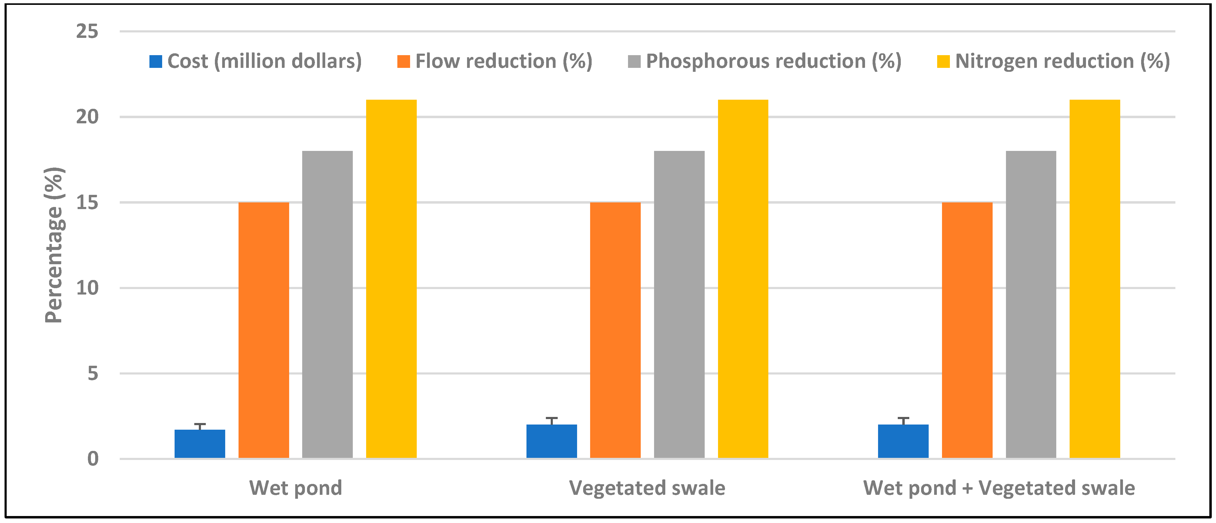
The results from this study indicate that the reduction of total phosphorus, total nitrogen, and runoff under current and future land use conditions can be achieved by using either treat and release or infiltration-based GI practices. Under the current (2018) land use, treat and release systems such as vegetated swales and wet ponds were the most cost-effective GI practices to achieve TMDL requirements at USD 1.5 million. However, vegetated swales only occupied 6 acres of land as opposed to 7 acres under wet ponds. Under the future land use change A1B scenario projections, both vegetated swales were cost-effective at USD 1.5 million. However, if land area is a constraint, then building bioretention cells at USD 2 million will be effective, given it only takes 3 acres of land compared to vegetated swales that will occupy 8 acres. Similarly, under B1 land use projections, porous pavements were the cost-effective solution at USD 1.5 million. These results are consistent with [24] Gao et al. (2015), who used the SUSTAIN model and found the minimum costs to reduce Chemical Oxygen Demand (COD) by 40%, total nitrogen by 30%, and total phosphorus by 50% in the city of Ma’anshan, China, was of similar order in magnitude, at USD 3.96 million.
To restore the water quality of the Arroyo Colorado River to acceptable levels, it is pertinent that stakeholders prioritize reduction based on analysis of the future land use scenarios. If measures will be taken across the watershed for economic sustainability, it is recommended that infiltration-based GI practices (porous pavement) be considered under the B1 scenario of land use since it enables complete compliance with TMDL regulations for nitrogen and phosphorus by the year 2050 in a cost-effective manner. The costs required for nutrient reduction under the B1 land use scenario are slightly lower than those for the A1B scenario because holistic sustainability measures are enforced in the watershed to minimize the effects of projected land use change.
Under the A1B land use scenario, tradeoffs would have to be made since this scenario represents a situation in which there is rapid growth in technology, economic growth, and population until the mid-century and declines after the introduction of more efficient technologies, thus creating a balance between the use of fossil fuels and non-fossil fuel sources of energy. The introduction of more efficient technologies may have an impact on the management of both agricultural and urban watersheds, thus reducing the likelihood of flooding and water quality deterioration, but the impact could not be predicted here.
In addition, the results show that when a combination of stormwater management actions are implemented, such as residue management, irrigation BMPs, nutrient management, seasonal residue management, land leveling at the farm level, and urban BMPs in urban areas, the costs and number of BMPs required to meet TMDL targets significantly reduces. Therefore, it is important to note that such stormwater management actions are relatively cheaper and provide significant cost savings in the long run for local governments and cities. This is consistent with other studies such as [15,48,49]. Cost analysis indicated that implementing a single BMP was relatively cheaper than implementing a combination of multiple BMPs to achieve the TMDL requirements. The mitigation costs under the future land use change scenarios were similar to those needed to achieve TMDL requirements under the current land use change. Most cost-effective strategies cost between USD 1.5 to 2 million, including other management practices, for water quality mitigation.
In terms of both reduced area and cost requirements, the use of bioretention cells is a feasible option to achieve TMDL targets. This can be attributed to the design of each bioretention cell with a filter material and pretreatment unit that removes excessive nutrients. The design of the bioretention systems in this study assumed that there is a pretreatment unit with filter material that removes some particulate phosphorus. In contrast, a portion of the dissolved phosphorus is assumed to be removed by the plants on the side slopes of the bioretention cell. The filter materials can be selected based on locally available cost-effective materials. For example, relatively coarser materials such as river rocks were effective in flood-prone areas for reducing stormwater flow and improving water quality [41,50,51,52]. This research proposes a combination of bioretention in urban areas and nutrient management in agricultural fields for the achievement of TMDL targets in the shortest time possible. This calls for a holistic approach between urban stakeholders and agricultural field owners in implementing the action items set forth in [8].
This study provides valuable information for stakeholders and city managers to make decisions about implementing GI strategies in achieving TMDL requirements. There are some limitations of this study. For example, the future land use projection maps were resampled from 250 m to 30 m for implementing the models, which can induce some uncertainties in estimating land use change impacts. It is recommended that the combined effects of climate and land use, along with a lifecycle analysis, be studied for the Arroyo Colorado Watershed as well as other similar semi-arid watersheds to develop holistic approaches for the future. There is also uncertainty in the cost requirements for the different BMPs since the costs used to run the model were purely conservative to determine the minimum investment required by the cities in the watershed to achieve TMDL targets within the next 25–30 years. In the future, lifecycle assessment for GI practices can be assessed under different hydroclimatic settings. Given that the performance of GI practices can change with time and different maintenance schedules, such information can be modelled by updating different parameters of the GI practices over their life-spans. In addition, it will be interesting to study how changes in the magnitude and frequency of extreme events can affect the performance of the GI practices, which will be explored in the near future.

5. Conclusions

This study analyzed the performance of green infrastructure under two land use scenarios, in the Arroyo Colorado River, using a coupled SWAT-SUSTAIN model. It showed that while the agricultural land use percentage will decrease by mid-century, the urban land use percentage will increase compared to current land use (2018). Under the current (2018) land use, vegetated swales over 6 acres were the most cost-effective GI practices to achieve TMDL requirements at USD 1.5 million. In future land use scenarios, vegetative swales and porous pavements were cost effective in the A1B and B1 scenarios. However, the bioretention cell was most effective per unit area. If suitable green infrastructure practices are optimally placed in the watershed, there would be a reduction of flooding events and pollution of the river, which would lead to the restoration of the river to acceptable levels and the elimination of impairment. The SWAT-SUSTAIN model is a valuable tool that can be utilized in other watersheds in semi-arid hydroclimatic conditions, particularly undergoing land use changes. The coupled model is helpful in estimating optimal costs in meeting target reductions in runoff and pollutant concentrations. These results are crucial to decision-makers, planners, and stakeholders in the watershed as they determine how to allocate stormwater resources in planning for the future of the watershed. Such an approach can be adopted in other watersheds, regions, and countries.

Author Contributions

Conceptualization, P.M. and T.S.; methodology, P.M. and T.S.; data analysis, P.M. and T.S.; writing and editing, P.M. and T.S.; calibration and implementation of models, P.M.; supervision and project administration, T.S.; funding acquisition, T.S. All authors have read and agreed to the published version of the manuscript.

Funding

This work was supported by the Texas Commission on Environmental Quality (contract # 582-19-90203) and the National Science Foundation for Research Excellence in Science and Technology—Center for Sustainable Water Use (CREST-SWU) under Grant Number 1914745.

Data Availability Statement

Data is contained within this article. Additional data and model outputs are available at https://drive.google.com/drive/folders/1kN5Ig6AA9IfKl5bUEoO-sW2-COQkXujx?usp=drive_link (accessed on 18 May 2025).

Conflicts of Interest

The authors declare no conflict of interest.

References

  1. Clark, G.M.; Mueller, D.K.; Mast, M.A. Nutrient concentrations and yields in undeveloped stream basins of the United States. J. Am. Water Resour. Assoc. 2000, 36, 849–860. [Google Scholar] [CrossRef]
  2. Greene, S.B.D.; LeFevre, G.H.; Markfort, C.D. Improving the spatial and temporal monitoring of cyanotoxins in Iowa lakes using a multiscale and multi-modal monitoring approach. Sci. Total Environ. 2021, 760, 143327. [Google Scholar] [CrossRef] [PubMed]
  3. Gallo, E.; Bell, C.; Mika, K.; Gold, M.; Hogue, T.S. Stormwater Management Options and Decision-Making in Urbanized Watersheds of Los Angeles, California. J. Sustain. Water Built Environ. 2020, 6, 04020003. [Google Scholar] [CrossRef]
  4. McGrane, S.J. Impacts of urbanisation on hydrological and water quality dynamics, and urban water management: A review. Hydrol. Sci. J. 2016, 61, 2295–2311. [Google Scholar] [CrossRef]
  5. Enciso, J.; Nelson, S.D.; Perea, H.; Uddameri, V.; Kannan, N.; Gregory, A. Impact of residue management and subsurface drainage on non-point source pollution in the Arroyo Colorado. Sustain. Water Qual. Ecol. 2014, 3–4, 25–32. [Google Scholar] [CrossRef]
  6. Kuwayama, Y.; Olmstead, S.M.; Wietelman, D.C.; Zheng, J. Trends in nutrient-related pollution as a source of potential water quality damages: A case study of Texas, USA. Sci. Total Environ. 2020, 724, 137962. [Google Scholar] [CrossRef]
  7. Kusnierz, P.C.; Alford, B.; Pierce, R.; Tracy, B.H.; Jager, H.I.; Lomnicky, G. Section 303 (d) of the Clean Water Act: What does it mean for fisheries? Fisheries 2025, 50, 19–26. [Google Scholar] [CrossRef]
  8. Flores, J.; Wagner, K.; Gregory, L.A.; Benavides, J.; Cawthon, T. Update to the Arroyo Colorado Watershed Protection Plan. 2017. Available online: https://arroyocolorado.org/media/wwmmsqzx/arroyo-colorado-wpp-final-optimized.pdf (accessed on 15 March 2023).
  9. Texas Commission on Environmental Quality (TCEQ). Texas Integrated Report for Clean Water Act Sections 305(b) and 303(d). 2020. Available online: https://wayback.archive-it.org/414/20210527150949/https://www.tceq.texas.gov/assets/public/waterquality/swqm/assess/20txir/2020_Basin22.pdf (accessed on 15 March 2023).
  10. Tim, D.; Shuster, W.; Hunt, W.F.; Ashley, R.; Butler, D.; Arthur, S.; Trowsdale, S.; Barraud, S.; Semadeni-Davies, A.; Bertrand-Krajewski, J.-L.; et al. SUDS, LID, BMPs, WSUD and more—The evolution and application of terminology surrounding urban drainage. Urban Water J. 2014, 12, 525–542. [Google Scholar] [CrossRef]
  11. Purvis, R.A.; Winston, R.J.; Hunt, W.F.; Lipscomb, B.; Narayanaswamy, K.; McDaniel, A.; Lauffer, M.S.; Libes, S. Evaluating the Water Quality Benefits of a Bioswale in Brunswick County, North Carolina (NC), USA. Water 2018, 10, 134. [Google Scholar] [CrossRef]
  12. Chen, C.; Guo, W.; Ngo, H.H. Pesticides in stormwater runoff—A mini review. Front. Environ. Sci. Eng. 2019, 13, 72. [Google Scholar] [CrossRef]
  13. Ahiablame, L.M.; Engel, B.A.; Chaubey, I. Effectiveness of Low Impact Development Practices: Literature Review and Suggestions for Future Research. Water Air Soil Pollut. 2012, 223, 4253–4273. [Google Scholar] [CrossRef]
  14. Dutta, A.; Torres, A.S.; Vojinovic, Z. Evaluation of Pollutant Removal Efficiency by Small-Scale Nature-Based Solutions Focusing on Bio-Retention Cells, Vegetative Swale, and Porous Pavement. Water 2021, 13, 2361. [Google Scholar] [CrossRef]
  15. Kannan, N. Water Quality Modeling of An Agricultural Watershed With Best Management Practices. Int. J. Res. Eng. Technol. 2014, 3, 553–564. [Google Scholar] [CrossRef]
  16. Arnold, J.G.; Moriasi, D.N.; Gassman, P.W.; Abbaspour, K.C.; White, R.; Srinivasan, C.; Santhi, R.D.; Harmel, A.; van Griensven, M.W.; Van, L.; et al. SWAT: Model Use, Calibration, and Validation. Trans. ASABE 2012, 55, 1491–1508. [Google Scholar] [CrossRef]
  17. Kannan, N.; Jeong, J.; Srinivasan, R. Hydrologic Modeling of a Canal-Irrigated Agricultural Watershed with Irrigation Best Management Practices: Case Study. J. Hydrol. Eng. 2011, 16, 746–757. [Google Scholar] [CrossRef]
  18. Okiria, E.; Okazawa, H.; Noda, K.; Kobayashi, Y.; Suzuki, S.; Yamazaki, Y. A Comparative Evaluation of Lumped and Semi-Distributed Conceptual Hydrological Models: Does Model Complexity Enhance Hydrograph Prediction? Hydrology 2022, 9, 89. [Google Scholar] [CrossRef]
  19. Zhang, Z.; Montas, H.; Shirmohammadi, A.; Leisnham, P.T.; Negahban-Azar, M. Impacts of Land Cover Change on the Spatial Distribution of Nonpoint Source Pollution Based on SWAT Model. Water 2023, 15, 1174. [Google Scholar] [CrossRef]
  20. Velásquez, R.A. Application of WinSLAMM to Evaluate the Effect of Green Infrastructure Implementation in Northern Utah. Ph.D. Thesis, Utah State University, Logan, UT, USA, 2018. Volume 7405. [Google Scholar]
  21. Shoemaker, L.; Riverson, J.; Alvi, K.; Zhen, J.X.; Murphy, R. Report on Enhanced Framework (SUSTAIN) and Field Applications for Placement of BMPs in Urban Watersheds (EPA 600/R-11/144; p. 150). USEPA. 2011. Available online: https://nepis.epa.gov/Exe/ZyNET.exe/P100DEWI.TXT?ZyActionD=ZyDocument&Client=EPA&Index=2011+Thru+2015&Docs=&Query=&Time=&EndTime=&SearchMethod=1&TocRestrict=n&Toc=&TocEntry=&QField=&QFieldYear=&QFieldMonth=&QFieldDay=&IntQFieldOp=0&ExtQFieldOp=0&XmlQuery=&File=D%3A%5Czyfiles%5CIndex%20Data%5C11thru15%5CTxt%5C00000004%5CP100DEWI.txt&User=ANONYMOUS&Password=anonymous&SortMethod=h%7C-&MaximumDocuments=1&FuzzyDegree=0&ImageQuality=r75g8/r75g8/x150y150g16/i425&Display=hpfr&DefSeekPage=x&SearchBack=ZyActionL&Back=ZyActionS&BackDesc=Results%20page&MaximumPages=1&ZyEntry=1&SeekPage=x&ZyPURL (accessed on 15 March 2023).
  22. Shoemaker, L.; Riverson, J.; Alvi, K.; Zhen, J.; Paul, S.; Rafi, T. SUSTAIN—A Framework for Placement of Best Management Practices in Urban Watersheds to Protect Water Quality. Report. 2009. Available online: https://nepis.epa.gov/Exe/ZyNET.exe/P1005IFG.TXT?ZyActionD=ZyDocument&Client=EPA&Index=2006+Thru+2010&Docs=&Query=&Time=&EndTime=&SearchMethod=1&TocRestrict=n&Toc=&TocEntry=&QField=&QFieldYear=&QFieldMonth=&QFieldDay=&IntQFieldOp=0&ExtQFieldOp=0&XmlQuery=&File=D%3A%5Czyfiles%5CIndex%20Data%5C06thru10%5CTxt%5C00000012%5CP1005IFG.txt&User=ANONYMOUS&Password=anonymous&SortMethod=h%7C-&MaximumDocuments=1&FuzzyDegree=0&ImageQuality=r75g8/r75g8/x150y150g16/i425&Display=hpfr&DefSeekPage=x&SearchBack=ZyActionL&Back=ZyActionS&BackDesc=Results%20page&MaximumPages=1&ZyEntry=1&SeekPage=x&ZyPURL (accessed on 15 March 2023).
  23. Kannan, N. SWAT Modeling of The Arroyo Colorado Watershed. Technical Report No. 426. 2012, p. 51. Available online: https://oaktrust.library.tamu.edu/server/api/core/bitstreams/5cfdafab-5165-4362-b261-3aa827620443/content (accessed on 15 March 2023).
  24. Gao, J.; Wang, R.; Huang, J.; Liu, M. Application of BMP to urban runoff control using SUSTAIN model: Case study in an industrial area. Ecol. Model. 2015, 318, 177–183. [Google Scholar] [CrossRef]
  25. Dewitz, J.; U.S. Geological Survey. National Land Cover Database (NLCD) 2019 Products. U.S. Geological Survey Data Release, ver. 2.0, June 2021. Available online: https://doi.org/10.5066/P9KZCM54 (accessed on 15 March 2023).
  26. International Boundary and Water Commission (IBWC). Data—USIBWC Water Data. Available online: https://waterdata.ibwc.gov/Data/Chart/Interval/Latest (accessed on 15 March 2020).
  27. Texas Commission on Environmental Quality (TCEQ). Surface Water Quality Web Reporting Tool. 2019. Available online: https://www80.tceq.texas.gov/SwqmisPublic/index.htm (accessed on 15 October 2021).
  28. United States Department of Agriculture (USDA). Soil Survey Staff. Gridded Soil Survey Geographic (gSSURGO) Database for Texas. Natural Resources Conservation Service. Available online: https://gdg.sc.egov.usda.gov/ (accessed on 15 March 2023).
  29. Thornton, M.M.; Shrestha, R.; Wei, Y.; Thornton, P.E.; Kao, S.-C.; Wilson, B.E. Daymet: Annual Climate Summaries on a 1-km Grid for North America, Version 4 R1. ORNL DAAC, Oak Ridge, Tennessee, USA. Available online: https://doi.org/10.3334/ORNLDAAC/2130 (accessed on 15 March 2023).
  30. U.S. Geological Survey (USGS). National Hydrography Dataset ver. USGS National Hydrography Dataset Best Resolution (NHD) for Hydrologic Unit (HU) 4–2001 (published 20191002). Available online: https://www.usgs.gov/national-hydrography/national-hydrography-dataset (accessed on 15 March 2019).
  31. Texas Commission on Environmental Quality (TCEQ). Pitted Outfalls Shapefile. Available online: http://www.tceq.texas.gov/gis/download-tceq-gis-data (accessed on 15 October 2021).
  32. Abbaspour, K.C. SWAT Calibration and Uncertainty Programs. SWAT-CUP: SWAT Calibration and Uncertainty Programs—User Manual. 2015. Available online: https://swat.tamu.edu/media/114860/usermanual_swatcup.pdf (accessed on 15 March 2023).
  33. Moriasi, D.N.; Gitau, M.W.; Pai, N.; Daggupati, P. Hydrologic and water quality models: Performance measures and evaluation criteria. Trans. ASABE 2015, 58, 1763–1785. [Google Scholar] [CrossRef]
  34. Abbaspour, K.C.; Rouholahnejad, E.; Vaghefi, S.; Srinivasan, R.; Yang, H.; Kløve, B. A continental-scale hydrology and water quality model for Europe: Calibration and uncertainty of a high-resolution large-scale SWAT model. J. Hydrol. 2015, 524, 733–752. [Google Scholar] [CrossRef]
  35. U.S. Environmental Protection Agency (USEPA). Low Impact Development Stormwater Control Cost Estimation Analysis. RTI International and Geosytec Consultants Report, US EPA Contract No. EP-C-11-036. 2015. Available online: https://pasteur.epa.gov/uploads/10.23719/1510483/documents/LID%20Cost%20Analysis_Report_National%20SWC_2015.pdf (accessed on 15 March 2023).
  36. Water Research Foundation. Urban Stormwater BMP Database. International Stormwater BMP Database. Available online: https://bmpdatabase.org/urban (accessed on 18 October 2021).
  37. Sohl, T.L.; Sayler, K.L.; Bouchard, M.A.; Reker, R.R.; Freisz, A.M.; Bennett, S.L.; Sleeter, B.M.; Sleeter, R.R.; Wilson, T.; Soulard, C.; et al. Conterminous United States Land Cover Projections—1992 to 2100. 2018, U.S. Geological Survey. Available online: https://www.sciencebase.gov/catalog/item/5b96c2f9e4b0702d0e826f6d (accessed on 15 March 2023).
  38. Sohl, T.L.; Sayler, K.L.; Bouchard, M.A.; Reker, R.R.; Freisz, A.M.; Bennett, S.L.; Sleeter, B.M.; Sleeter, R.R.; Wilson, T.; Soulard, C.; et al. Spatially explicit modeling of 1992–2100 land cover and forest stand age for the conterminous United States. Ecol. Appl. 2014, 24, 1015–1036. [Google Scholar] [CrossRef] [PubMed]
  39. Intergovernmental Panel on Climate Change (IPCC). Scenario Data for the Atmospheric Environment. Available online: https://www.ipcc-data.org/sim/gcm_clim/SRES_TAR/ddc_sres_emissions.html (accessed on 15 March 2023).
  40. Jayasooriya, V.M.; Ng, A.W.M.; Muthukumaran, S.; Perera, C.B.J. Optimization of Green Infrastructure Practices in Industrial Areas for Runoff Management: A Review on Issues, Challenges and Opportunities. Water 2020, 12, 1024. [Google Scholar] [CrossRef]
  41. Salha, A.A. Nonpoint Source Pollution Control Using a Multi-Objective Optimization Tool for Best Management Practices Selection and Spatial Placement in the Lower Bear River Watershed, Utah. Ph.D. Thesis, Utah State University, Logan, UT, USA, 2020. [Google Scholar]
  42. Mahmoud, A.; Alam, T.; Yeasir, A.R.M.; Sanchez, A.; Guerrero, J.; Jones, K.D. Evaluation of field-scale stormwater bioretention structure flow and pollutant load reductions in a semi-arid coastal climate. Ecol. Eng. 2019, 1, 100007. [Google Scholar] [CrossRef]
  43. Dari, B.; Nair, V.D.; Colee, J.; Harris, W.G.; Mylavarapu, R. Estimation of phosphorus isotherm parameters: A simple and cost-effective procedure. Front. Environ. Sci. 2015, 3, 70. Available online: https://www.frontiersin.org/articles/10.3389/fenvs.2015.00070 (accessed on 1 May 2025). [CrossRef]
  44. Hou, J.; Zhu, M.; Wang, Y.; Sun, S. Optimal spatial priority scheme of urban LID-BMPs under different investment periods. Landsc. Urban Plan. 2020, 202, 103858. [Google Scholar] [CrossRef]
  45. Pease, L.M.; Oduor, P.; Padmanabhan, G. Estimating sediment, nitrogen, and phosphorous loads from the Pipestem Creek watershed, North Dakota, using AnnAGNPS. Comput. Geosci. 2010, 36, 282–291. [Google Scholar] [CrossRef]
  46. Urbonas, B.R. Effectiveness of Urban Stormwater BMPs in Semi-Arid Climates. Regional Conference on: Experience with Best Management practices in Colorado. April 2003. Available online: https://mail.uwtrshd.com/assets/effectiveness-of-bmps-in-semi-arid-climates.pdf (accessed on 1 May 2025).
  47. Texas A&M Agrilife Extension Report. Available online: https://rainwaterharvesting.tamu.edu/rangeland-watersheds/ (accessed on 15 February 2025).
  48. Zhu, N.; Yan, Y.; Bai, K.; Zhang, J.; Wang, C.; Wang, X.; Xu, D.; Liu, J.; Xin, X.; Chen, J. Conversion of croplands to shrublands does not improve soil organic carbon and nitrogen but reduces soil phosphorus in a temperate grassland of northern China. Geoderma 2023, 432, 116407. [Google Scholar] [CrossRef]
  49. Pokhrel, B.K.; Paudel, K.P. Assessing the Efficiency of Alternative Best Management Practices to Reduce Nonpoint Source Pollution in a Rural Watershed Located in Louisiana, USA. Water 2019, 11, 1714. [Google Scholar] [CrossRef]
  50. Abduljaleel, Y.; Demissie, Y. Identifying Cost-Effective Low-Impact Development (LID) under Climate Change: A Multi-Objective Optimization Approach. Water 2022, 14, 3017. [Google Scholar] [CrossRef]
  51. Liu, A.; Egodawatta, P.; Goonetilleke, A. Ranking Three Water Sensitive Urban Design (WSUD) Practices Based on Hydraulic and Water Quality Treatment Performance: Implications for Effective Stormwater Treatment Design. Water 2022, 14, 1296. [Google Scholar] [CrossRef]
  52. Alam, T.; Mahmoud, A.; Jones, K.D.; Bezares-Cruz, J.C.; Guerrero, J. WinSLAMM simulation of hydrologic performance of permeable pavements—A case study in the semi-arid Lower Rio Grande Valley of South Texas, United States. Water 2019, 11, 1865. [Google Scholar] [CrossRef]
Figure 1. Map showing: (A) Texas and (B) location of the Arroyo Colorado River basin along with three selected subwatersheds in South Texas, U.S.
Water 17 01565 g001
Figure 2. Comparison of the observed and the SWAT model-simulated streamflow at a monthly time step.
Water 17 01565 g002
Figure 3. Comparison of observed and the SWAT model-simulated total nitrogen during 2013 to 2015 at station 13,079 with an R2 of 0.81.
Water 17 01565 g003
Figure 4. Same as Figure 3, but it has an R2 of 0.85 for total phosphorus.
Water 17 01565 g004
Figure 5. Comparison of SWAT and SUSTAIN simulated streamflow during 2013 to 2020.
Water 17 01565 g005
Figure 6. Effects of selected treat and release GI practices on runoff volume, total nitrogen, phosphorus, and their costs under the current (2018) land use scenario during the 2013–2020 period. The error bars for the costs (shown in blue) represent the upper limits of the solutions under each scenario.
Water 17 01565 g006
Figure 7. Infiltration GI practices under the current land use (2018) scenario using rainfall data from 2013 to 2020. The error bars for the costs represent the upper limits of the solutions for each scenario.
Water 17 01565 g007
Figure 8. Comparison between (A) current (2018) and future (2050) land use for the three subwatersheds under (B) A1B and (C) B1 scenarios.
Water 17 01565 g008
Figure 9. Percentage land use comparison between 2018 and 2050 FORE-SCE land use for A1B and B1 scenarios.
Water 17 01565 g009
Figure 10. Treat and release GI practices under the A1B land use scenario using rainfall data from 2013 to 2020.
Water 17 01565 g010
Figure 11. Infiltration GI practices under the A1B land use scenario using rainfall data from 2013 to 2020. The error bars for the costs represent the upper limits of the solutions for each scenario.
Water 17 01565 g011
Figure 12. Treat and release GI practices under the B1 land use scenario using rainfall data from 2013 to 2020. The error bars for the costs represent the upper limits of the solutions for each scenario.
Water 17 01565 g012
Figure 13. Infiltration GI practices under the B1 land use scenario using rainfall data from 2013 to 2020. The error bars for the costs represent the upper limits of the cost solutions for each scenario.
Water 17 01565 g013
Table 1. Land uses and their relative percentage breakdown in the three selected subwatersheds based on the 2018 NLCD land use.
Relative Fractional Land Use Composition (%)
Land Use/Land CoverSubwatershed 1 (Mission Area)Subwatershed 2 (Weslaco Area)Subwatershed 3 (Mercedes Area)
Open Water0.571.502.07
Developed, Open Space8.055.574.73
Developed, Low Intensity14.9711.376.73
Developed, Medium Intensity13.046.703.52
Developed, High Intensity4.530.830.39
Barren Land0.480.600.54
Deciduous Forest1.190.730.56
Evergreen Forest0.110.030.06
Mixed Forest0.840.270.03
Shrub/Scrub2.722.818.64
Herbaceous1.943.373.23
Hay/Pasture5.114.785.30
Cultivated Crops45.9360.7262.94
Woody Wetlands0.220.320.84
Emergent Herbaceous Wetlands0.310.410.41
Total100.00100.00100.00
Table 2. Data and sources used for implementing the SWAT and SUSTAIN models.
DataSources
Light Detection and Ranging (LiDAR) dataTexas Natural Resources Information System
StreamflowInternational Boundary and Water Commission (IBWC) gage
08470400 from 2012–2020 time period [26]
Water qualitySurface Water Quality Monitoring (SWQM) Station # 13,079 was used for total nitrogen and phosphorus data [27]. A few missing data at station # 13,079 were filled using the average values for neighboring stations (13,084 and 13,081) during 2012–2015.
Land useNational Land Cover Dataset (NLCD) 2018, 30 m resolution [25]
SoilsGridded Soil Survey Geographic (gSSURGO), 10 m × 10 m data for Texas [28]
Rainfall and Meteorology forcingsDaymet Daily Surface Weather and Climatological Summaries for 2012–2020 [29]
StreamsNational Hydrography Dataset (NHD) Plus [30]
Wastewater outfallsTexas Commission on Environmental Quality (TCEQ) Permitted Outfalls shapefiles [31]
Table 3. SWAT-CUP calibration parameters and their ranges.
SWAT-CUP Parameter.Input FileDescription and Ranges in Brackets Proposed by [33]Values Used in This Study
CN2mgtInitial SCS runoff CN value for moisture condition II (±10%)1.15
GWQMNgwThe threshold depth of water in the shallow aquifer required for return flow to occur (0–1000)528
SOL_BDsolSoil bulk density 0.16
CH_S2rteAverage channel slope along channel length (±50%)1.84
ALPHA_BFgwBaseflow alpha factor (0.1–1.0)0.8
CH_N2rteManning’s n value for the main channel (0.008–0.3)0.24
MSK_CO1bsnWeighting factor for influence of normal flow on storage time constant (0.01–10)4.75
GW_DELAYgwGroundwater delay time (0–100)4.13
ESCObsnSoil evaporation compensation factor (0–1)0.38
EPCObsnPlant uptake compensation factor (0–1)0.34
CH_W2rteAverage width of the main channel at the top of the bank0.6
CH_L2rteLength of main channel0.63
SURLAGbsnSurface runoff lag coefficient (0.001–15)8.17
GW_REVAPgwGroundwater “revap” coefficient (0.02–0.1)0.02
SOL_AWCsolAvailable water capacity of the soil layer (±30%)−0.58
RCHRG_DPgwDeep aquifer percolation fraction (0.0–1.0)0.2
CH_K2rteEffective hydraulic conductivity of channel (mm/hr) (0.025–150)1.31
ALPHA_BNKrteBaseflow alpha factor for bank storage (days)0.5
OV_NhruManning’s n value for overland flow (0.05–0.8)0.12
MSK_CO2bsnWeighting factor for influence of low flow on storage time constant (0.01–10)5.74
SOL_KsolSaturated hydraulic conductivity (±30%)0.45
Table 4. SUSTAIN model parameters that were adjusted to match flow and water quality conditions with the SWAT simulated values as well as the observations.
ParameterRangeValues Used in This Study
Hydraulic conductivity0.06–1.42 in/h0.85 in/h
Depression Storage impervious surfaces0.05–0.1 inches0.09 inches
Depression Storage pervious surfaces0.2 inches0.2 inches
Manning’s roughness coefficient for impervious areas0.011–0.10.02
Manning’s roughness coefficient for pervious areas0.01–0.20.1
Table 5. Costs of components used in SUSTAIN based on [35].
GI Practice (Approximate Dimensions from [36]Component CostSUSTAIN Cost [35]
Bioretention (2070 ft × 1000 ft × 3 ft)Construction cost$10/square foot
Porous pavement (788 ft × 300 ft)Unit Cost$2/square foot
Vegetated swale (180 ft × 60 ft × 1.5 ft)Construction cost $4.5/square foot
Wet pond (200 ft × 100 ft × 3 ft)Construction cost$4.6/square foot
Table 6. GI practices modeled under corresponding land use scenarios.
Scenario 1—A1B Land Use Treat and Release GIs Scenario 2—A1B Land Use
Infiltration GIs
Scenario 3—Same as Scenario 1 (Column 1), but for B1 Land UseScenario 4—Same as Scenario 2 (Column 2), but for B1 Land Use
Wet pond Porous pavementWet pond Porous pavement
Vegetated swale Bioretention Vegetated swale Bioretention
Wet pond + Vegetated swale Porous pavement + Bioretention Wet pond + Vegetated swale Porous pavement + Bioretention
Table 7. Optimization results in acreage for GI practices in the three subwatersheds under current land use scenarios to achieve 18% removal of phosphorus from 0.69 mg/L and 21% removal of nitrogen from 0.445 mg/L.
BMP TypeOptimized Area (Acres) Needed to Meet TMDL Targets Under Each BMP Type Without Other Management Practices Total Cost ($)BMP UnitsOptimized Area (Acres) Needed to Meet TMDL Targets Under Each BMP Type When Used with Other Management Practices *Total Cost ($)BMP Units
Vegetated swale545 118,701,00011,018.5 61,500,000138.89
Bioretention436189,660,0009252,500,0001.2
Porous pavements42537,026,000157151,800,0007.6
Wet ponds985197,370,3609850 71,500,00075
* Nutrient management---12,00042,476-
* Terracing---130637-
* Residue management---140010,872-
* Subsurface drain---40002471-
Note: * Other management practices based on [15].
Table 8. Optimization results in acreage for GI practices in the three subwatersheds under A1B future land use scenarios to achieve 18% removal of phosphorus from 0.69 mg/L and 21% removal of nitrogen from 0.445 mg/L.
BMP TypeOptimized Area (Acres) Needed to Meet TMDL Targets Under Each BMP Type Without Other Management PracticesTotal Cost ($)BMP UnitsOptimized Area (Acres) Needed to Meet TMDL Targets Under Each BMP When Used with Other Management Practices *Total Cost ($)BMP Units
Vegetated swale20544,649,000372171,568,160145
Bioretention9641,760,00021 32,000,0001
Porous pavements35030,492,000169 202,000,0008
Wet ponds15030,056,4001600 153,000,000150
Note: * Other management practices shown in Table 7.
Table 9. Optimization results in acreage for GI practices in the three subwatersheds under B1 future land use scenarios to achieve 18% removal of phosphorus from 0.69 mg/L and 21% removal of nitrogen from 0.445 mg/L.
BMP TypeOptimized Area (Acres) Needed to Meet TMDL Targets Under Each BMP Without Other PracticesTotal Cost ($)BMP UnitsOptimized Area (Acres) Needed to Meet TMDL Targets When Used with Other Management Practices *Total Cost ($)BMP Units
Vegetated swale18941.164,2003703 82,000,000185
Bioretention8536,975,0001832,100,0001
Porous pavements21218,469,440152171,542,6727
Wet ponds10020,037,60060081,730,00087
Note: * Other management practices shown in Table 7.
Disclaimer/Publisher’s Note: The statements, opinions and data contained in all publications are solely those of the individual author(s) and contributor(s) and not of MDPI and/or the editor(s). MDPI and/or the editor(s) disclaim responsibility for any injury to people or property resulting from any ideas, methods, instructions or products referred to in the content.

