Adaptive PID Control of Hydropower Units Based on Particle Swarm Optimization and Fuzzy Inference

Abstract

Currently, fixed-parameter proportional–integral–derivative (PID) control is widely adopted by the governor of hydropower units (HPUs), which causes regulation performance to deteriorate during variable operating conditions. To solve this problem, a novel particle swarm optimization-based fuzzy PID (PSO-FPID) is proposed for the frequency regulation of HPUs. The segment linearization model of HPU is first established to reflect the changes in the operating conditions. On this basis, FPID is designed based on expert experience. The PID control parameters are optimized using PSO under different operating conditions to determine the optimal initial values of the FPID controller. To verify the effectiveness of the proposed PSO-FPID, its performance is compared and analyzed with the actual PID, FPID, and particle swarm optimization-based PID (PSO-PID) in the MATLAB/Simulink platform. The results show that the average adjust time of PSO-FPID is 16.60 s less than that of PID, 18.05 s less than that of FPID, and 0.23 s less than that of PSO-PID. PSO-FPID can maintain better control performance than the other methods under most operating conditions.

1. Introduction

1.1. Aims and Motivation

Large-scale integration of wind and solar power into the power grid with volatility and randomness will make the stability of voltage, frequency, and other indicators worse, which may cause the power system to operate safely and stably, and then trigger a serious “abandonment of wind, abandonment of solar” phenomenon [1]. HPUs are commonly used as peak-frequency regulation units because of their fast start and stop, high flexibility, and widely adjustable range. In the context of the new power system, the role assumed by hydropower is changing from a single generation to a combination of generation and regulation. However, a hydraulic turbine regulation system (HTRS) is characterized by nonlinearity, time-varying, and hydraulic–mechanical–electrical coupling, which not only needs to cope with frequent operating condition switching and load fluctuation but also needs to withstand the power impact brought by the grid connection of large-scale new energy in the actual operating process. These factors tend to produce large deviations in frequency, increasing the difficulty of grid stabilization and the control requirements for the HPU. Therefore, with the development of new power systems, the response speed, stability, and control accuracy of an HTRS are experiencing unprecedented challenges [2], and there is an urgent need to design intelligent controllers for HPUs adapted to variable operating conditions.

1.2. Literature Review

The control strategies of HPUs are mainly categorized into PID control strategy and intelligent control strategy. The research on PID control strategy mainly focuses on optimizing the PID parameters and improving the PID structure. The research on intelligent control strategies mainly includes fuzzy control, neural network control, and so on. The study of optimizing the PID parameters is divided into the selection and improvement of the optimization algorithms and the design of the optimization objectives. In terms of the selection and improvement of the optimization algorithms, the swarm intelligence optimization algorithm is based on the simulation of natural evolution or the group collaboration mechanism, which is widely used because it can significantly improve the efficiency and accuracy of parameter tuning [3]. Some research has focused on combining two or more intelligent algorithms to improve the efficiency and accuracy of these algorithms. The genetic algorithm and PSO algorithm have been combined to optimize the PID parameters to stabilize the frequency deviation of the two-area power system, reducing the overshoot and the adjust time of the frequency response [4]. Introducing the memory mechanism of the particle swarm algorithm based on the whale algorithm could speed up the convergence of whale groups [5]. In terms of the design of the optimization objectives, the integrated time and absolute error (ITAE) is used as a common objective function for optimizing the control parameters because its time-weighted term ensures rapidity and its integral absolute error component ensures stability [6]. Since the single performance index for the evaluation of the control system exists in one-sidedness, many scholars have combined dynamic indexes such as adjust time, overshooting, reverse regulation, and ITAE with weighting factors to form a composite objective function to further improve the comprehensive control performance. Fractional-order PID control can be applied directly in the control of HPUs [7], or it can be used in combination with other methods, such as fractional-order PID controllers based on intelligent optimization algorithms [8], fuzzy fractional-order PID controllers [9], and fuzzy fractional-order PID controllers based on intelligent optimization algorithms [10].

Fuzzy control research has mainly focused on the traditional fuzzy model and the Takagi–Sugeno fuzzy model. The traditional fuzzy model was widely used in various control systems, including the HTRS, dual-area multi-source power generation, and variable-pitch tidal current power generation systems, because it did not require an accurate mathematical model [11]. Fuzzy rules were automatically generated using an adaptive neuro-fuzzy inference system, effectively addressing the issue of predicting the energy characteristics of the Kaplan hydraulic turbine [12]. Similarly, fuzzy rules were applied by using an adaptive neuro-fuzzy inference system to solve the problem of frequency stability in the automatic power generation control of hydropower plants [13]. Optimized fuzzy rules and affiliation functions using genetic algorithms have been used to improve dynamic performance effectively [14]. The Takagi–Sugeno fuzzy model requires accurate mathematical modeling and provides better control performance compared to conventional PID controllers in the face of external disturbances [15,16]. In addition, the model can be combined with finite-time control to solve the control problem caused by the mechanical time delay of the HTRS [17]. Neural network control is mainly used to adjust the control parameters to improve the control performance, robustness, and online prediction of the state of the controlled object. A back-propagation neural network as a kind of network can be used to optimize the PID parameters online to improve the adaptability of the controller; it can also be combined with intelligent algorithms to overcome the problem of easily falling into local optimization [18]. In addition, it can effectively reduce the adjusting time and overshoot of the system dynamic process by combining the self-learning ability of the neural network with the inference ability of fuzzy control [19]. The integration of fuzzy controllers, digital twins, and neural networks can improve the operational efficiency of hydropower systems and enhance fault detection and load management [20]. Model-free adaptive control was used to achieve rapid unit startup by eliminating the dependence on accurate mathematical models [21]; the new predictive control had a smaller adjust time and rise time than the fixed-parameter PID control strategy currently used in hydropower plants [22]. Robust control was adapted to hydropower units with a high percentage of renewable energy grid, which can effectively improve the anti-disturbance capability of the hydraulic turbine regulation system [23,24]. S-curve control could effectively suppress reverse power regulation and power oscillation [25]. Hamiltonian additional damping control was used to improve the operational stability of the hydraulic turbine in the vibration region and to extend the load regulation range [26].

1.3. Research Gaps and Contributions

The main gaps in the current study are as follows: (1) Limitations of intelligent control applications. Compared to PID control, intelligent control, such as neural networks, can better deal with nonlinear systems but requires the establishment of an accurate model of the controlled object [27]. Model accuracy directly affects control performance. The accurate modeling of the hydraulic turbine regulation system is more difficult due to its multivariate coupling and time-varying characteristics. At the same time, due to the complex structure and large number of parameters, the high calculation cost of intelligent control, and the difficulty of setting the parameters, it is difficult to meet the requirements of real-time control and reliability for practical applications. In addition, the extensive state information of the controlled object is required for some intelligent controls, which is often difficult to obtain in practice, further limiting the engineering applications of such controls. (2) Weak adaptivity of the PID control. Compared with intelligent control, PID control is widely used in process control of hydropower units due to the simple control structure and clear physical meaning of parameters that are easy to optimize. However, a fixed-parameter mode is used for traditional PID control (a set of control parameters is often used after the unit is connected to the grid), and its control performance cannot always be optimized when the unit operates under variable operating conditions. In the context of the new electricity system, the increasing regulation burden caused by new energy and load fluctuations is undertaken by hydropower units. In this context, the unit probably runs well under one operating condition under the traditional PID control strategy, while the regulation performance may deteriorate or even become unstable under another operating condition. (3) Related studies lack consideration of full operating condition scenarios. Most of the research focuses on the optimal control of certain specific operating conditions of hydropower units, such as a certain power generation condition, no-load condition, start-up condition, and so on [28,29]. The excellent control performance of the unit under variable operating conditions is difficult to guarantee with the control strategies obtained in this way.

To solve the above problems, a new PSO-FPID controller is proposed in this paper to achieve adaptive regulation for the variable operating conditions of an HPU by combining PID initial value optimization and dynamic tuning. The main contribution of this paper is as follows: (1) The HTRS model is established for the HPU of a power station under 42 different operating conditions; (2) the PSO algorithm is used to optimize the initial value of the PID offline for each operating condition; (3) based on the optimal initial value of PID, fuzzy control is introduced to adjust the PID parameters online during the dynamic process, which further improves the regulated performance of the HTRS; and (4) a large number of comparative experiments are designed from different perspectives to verify that the proposed control strategy has the optimal comprehensive control performance under most operating conditions. In this paper, the main innovation is using PSO offline optimization to construct a nonlinear relationship between the optimal control parameters and the operating conditions. Furthermore, through this nonlinear relationship and fuzzy control, the initial values and increments of the PID control parameters are adjusted online to realize optimal control under different operating conditions. A large amount of state information about the object is not required for the fuzzy control used here, which mainly realizes the real-time fine-tuning of the control parameters without affecting the basic regulation performance of PID control. PSO is used to determine the initial values of the control parameters, mainly to ensure that the PID control has excellent basic regulation performance under different operating conditions.

1.4. Paper Organization

The rest of the paper is structured as follows. In Section 2, the mathematical model of the HTRS is established for frequency regulation under different operating conditions. In Section 3, a fuzzy control system is first designed. The PID parameter optimization based on the PSO algorithm and the ITAE index is presented under a certain operating condition. Based on this, a novel PSO-FPID controller adapted to the variable operating conditions of the HPU is proposed by combining the fuzzy inference, which adjusts the PID parameters online, and PSO, which optimizes the PID parameters offline. In Section 4, HTRS simulation models are established under four different control strategies, including PID, FPID, PSO-PID, and PSO-FPID. The performance of each control strategy is quantitatively analyzed under different operating conditions, which proves the effectiveness and superiority of the proposed control strategy. Section 5 summarizes the work.

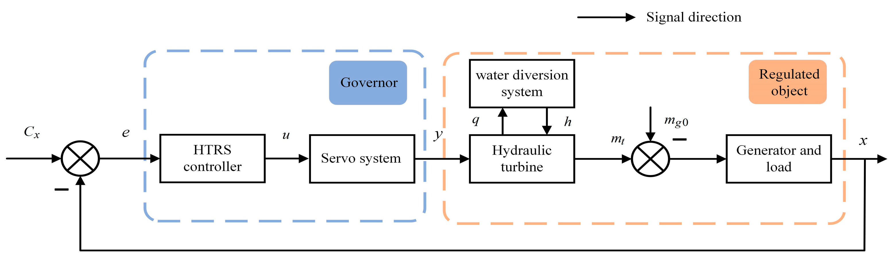
2. The HTRS Model

The core function of the HTRS is to maintain power system frequency stability by regulating the output power of the HPU to achieve precise control of rotational speed. From the perspective of system structure, the HTRS can be divided into two core components, governor and regulated object [30], which together constitute a time-varying, nonlinear, non-minimum phase, and strongly coupled closed-loop control system. The governor includes the controller and the servo system; the regulated objects include the hydraulic turbine, the water diversion system, the generator, and the load. The overall framework of the HTRS is shown in Figure 1.

2.1. Controller

The HTRS controller is responsible for processing the speed, guide vane opening (GVO), and power signals. Currently, the parallel PID model is widely adopted in HTRS, with the transfer function shown in Equation (1) [31].

$$G_c(s)={\displaystyle \frac{u(s)}{e(s)}}=K_P+{\displaystyle \frac{K_I}{s}}+{\displaystyle \frac{K_{D}s}{T_{d}s+1}}$$

(1)

where $G_c(s)$ is the transfer function of the controller; $u(s)$ is the output of the controller; $e(s)$ is the rotational speed deviation of the HTRS; s is the Laplace operator; $K_P,K_I,K_D$ are the proportional, integral, and differential gain, respectively; and $T_d$ is the differential time constant.

2.2. Servo System

The servo system is the core actuator of the governor. The output of the controller is converted into the movement signal of the servomotor through the hydraulic amplification of the servo system. The movable guide vane of the hydraulic turbine is driven by the servomotor to adjust the discharge. The transfer function of the servo system is shown in Equation (2).

$$G_y(s)={\displaystyle \frac{y(s)}{u(s)}}={\displaystyle \frac{1}{T_{y}s+1}}$$

(2)

where $y(s)$ is the GVO and $T_y$ is the reaction time constant of the servomotor.

2.3. Water Diversion System

Water diversion system models are categorized into elastic water hammer models and rigid water hammer models. In engineering applications, when the length of the pressure diversion pipe is short, it is assumed that there is no elastic effect between the water flow and the pipe wall. At the moment, the water and the pipe can be assumed to be rigid objects. In this paper, the rigid water hammer model is used, and the transfer function is shown in Equation (3) [32].

$$G_h(s)={\displaystyle \frac{h(s)}{q(s)}}=-T_{w}s$$

(3)

where $h(s)$ and $q(s)$ are the water head and discharge of the hydraulic turbine, respectively, and $T_w$ is the inertia time constant of the water flow.

2.4. Hydraulic Turbine

Hydraulic turbine models can be categorized into simplified linear models based on transfer coefficients and nonlinear models based on integrated characteristic curves. Under small fluctuating operating conditions, the linear model of the hydraulic turbine is shown in Equation (4) [33].

$$\left\{\begin{array}{l}{m}_t=e_{y}y+e_{x}x+e_{h}h\\ q=e_{qy}y+e_{qx}x+e_{qh}h\end{array}\right.$$

(4)

where $m_t$ is the hydraulic turbine torque; $e_y,e_x,e_h$ are the transfer coefficients of the torque to the GVO, rotational speed, and water head; $e_{qy},e_{qx},e_{qh}$ are the transfer coefficients of the discharge to the GVO, rotational speed, and water head; and $x$ is the rotational speed of the hydraulic turbine.

2.5. Hydraulic Turbine and Water Diversion System

Combining the hydraulic turbine and water diversion system model and taking into account that $e_{qx}$ of the Francis turbine is generally small and negligible, the transfer function of the hydraulic turbine and water diversion system can be shown in Equation (5).

$$G_t(s)={\displaystyle \frac{m_t(s)}{y(s)}}={\displaystyle \frac{e_y-(e_h{e}_{qy}-e_{qh}{e}_y)T_{w}s}{1+e_{qh}{T}_{w}s}}$$

(5)

2.6. Generator and Load

Generator models mainly include second-order, third-order, and fifth-order models. In power system analysis, third-order and higher models of generators are used if the dynamics of the excitation system and the role of the rotor damping windings are taken into account. When the effect of electrical transient processes is not considered, the first-order model of the generator is selected only to reflect the motion of the rotor. Combining the self-regulating ability of the hydraulic turbine and generator load, the transfer function of the generator and load is shown in Equation (6).

$$G_g(s)={\displaystyle \frac{x(s)}{m_t(s)-m_{g0}(s)}}={\displaystyle \frac{1}{T_{a}s+(e_g-e_x)}}$$

(6)

where $m_{g0}(s)$ is the load torque, $T_a$ is the inertia time constant of the unit, and $e_g$ is the load self-regulation coefficient.

3. Adaptive Control of Operating Conditions for an HPU

3.1. PID Control

Since the computer control is sampling control, the discrete PID control algorithm is adopted in this paper, as shown in Equation (7).

$$u(k)=K_{P}e\left(k\right)+K_I\Delta T{\displaystyle \sum _{j=0}^{k}e}\left(j\right)+{\displaystyle \frac{K_D}{\Delta T}}\left[e\left(k\right)-e\left(k-1\right)\right]$$

(7)

where $\Delta T$ is the sampling period; $K_P,K_I,K_D$ are the proportional, integral, and differential gains, respectively; $e$ is the system deviation signal; k denotes the kth sampling moment; and j is a loop variable.

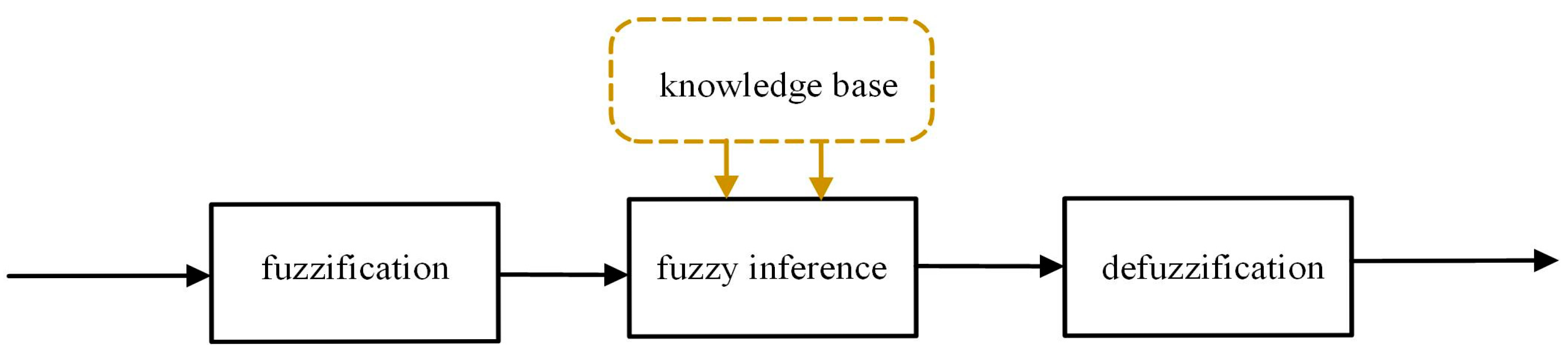
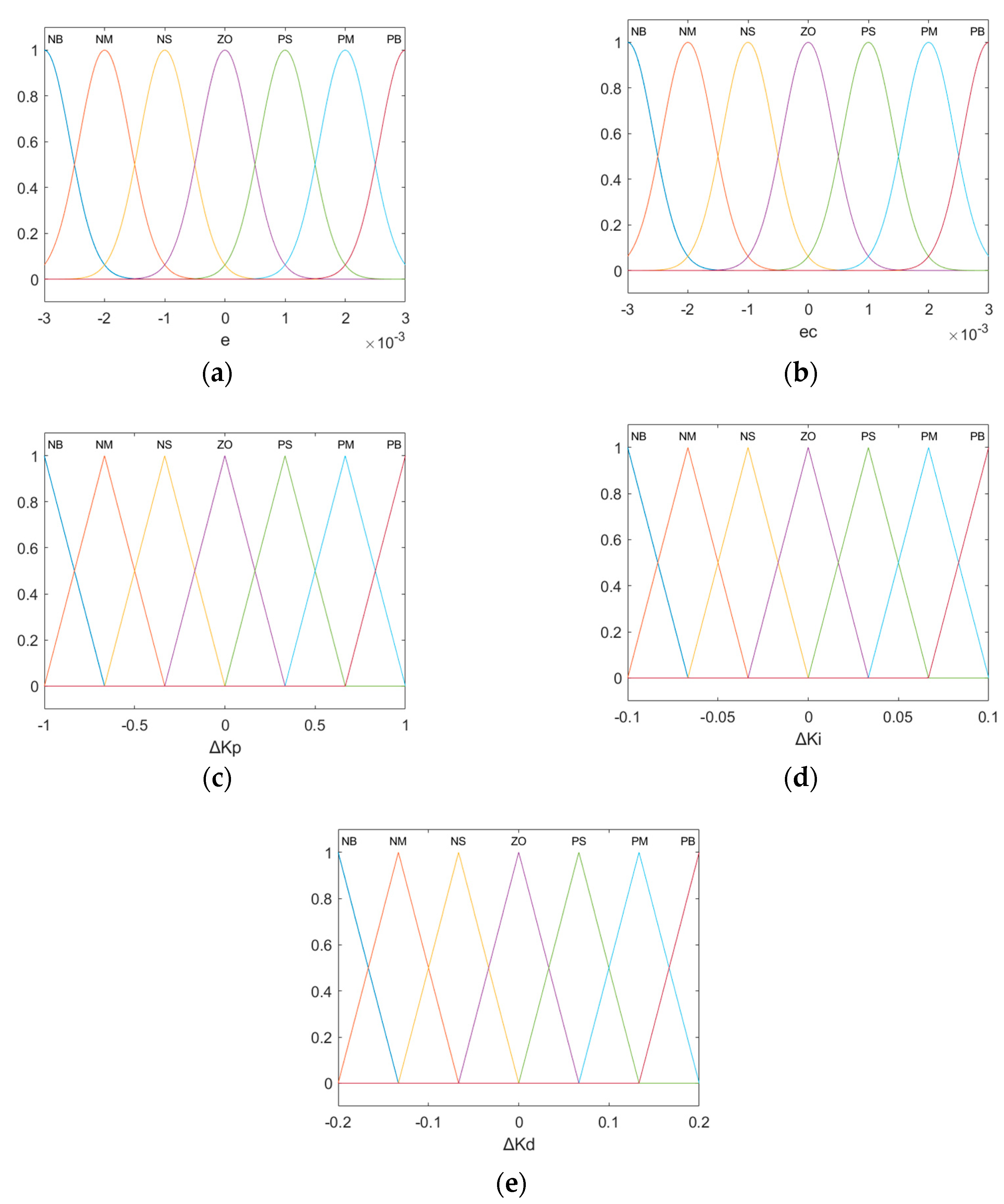
3.2. Fuzzy Control

In the field of intelligent control, fuzzy control was developed based on fuzzy mathematics. It realizes the control of digital quantities through the use of fuzzification, language variable description, and fuzzy inference mechanisms [34]. This control model based on expert experience not only reduces the complexity of control system modeling but also improves the adaptability and robustness of control. The fuzzy controller consists of four parts: fuzzification, knowledge base, fuzzy inference, and defuzzification. Its structure is shown in Figure 2.

The design of the fuzzy controller mainly includes the selection of the membership function and the formulation of fuzzy inference rules. In the design of the fuzzy controller for the HTRS, the inputs are the error $e$ and the change rate of the speed deviation $ec$, and the output is the amount of change in the control parameters $\Delta K_p,\Delta K_i,\Delta K_d$. Based on experience, the membership functions of the input parameters are chosen as $“gaussmf”$, and the domains are all set to [−0.003, 0.003]; the membership functions of the output parameters are chosen as $“trimf”$, with the domains of [−1, 1] for $\Delta K_p$, [−0.1, 0.1] for $\Delta K_i$, and [−0.2, 0.2] for $\Delta K_d$. The seven fuzzy levels are NB, NM, NS, ZO, PS, PM, and PB [35]. The membership functions of the input and output parameters are shown in Figure 3. Based on the related literature and experience, the fuzzy inference surfaces of the output parameters are designed as shown in Figure 4. The basic idea of fuzzy inference is as follows: In the early stage, due to the rapidity required for the HTRS, $\Delta K_p$ and $\Delta K_d$ are set to larger values, and $\Delta K_i$ is set to a smaller value. In the middle stage, $\Delta K_p$ increases appropriately to eliminate errors quickly, $\Delta K_i$ decreases appropriately to prevent integral saturation, and $\Delta K_d$ decreases appropriately to avoid oscillations. In the late stage, for eliminating static errors and ensuring a certain degree of rapidity, $\Delta K_p$ decreases appropriately while $\Delta K_i$ and $\Delta K_d$ increases appropriately.

3.3. The Optimization of Control Parameters Based on the Particle Swarm Algorithm

In the PSO algorithm, each particle can be represented by a velocity vector $v_i$, position vector $x_i$, and individual optimal position $pbes{t}_i$, which describes the unique state of motion. The velocity vector $v_i$ of the particle determines the direction of its motion and influences the distance of its motion in every iteration. There are two key reference positions in the particle swarm: the historical optimal position of the individual, denoted by $pbes{t}_i$, and the historical optimal position of the population, denoted by $gbes{t}_i$. $pbes{t}_i$ reflects the optimal solution found during particle motion, and $gbes{t}_i$ reflects the optimal solution in the current population [36]. On the one hand, these two reference mechanisms enable the particles to perform the local search according to $pbes{t}_i$, and on the other hand, they enable the particles to follow $gbes{t}_i$ for a global large-scale exploitation. For the $k+1$th iteration, Equation (8) can be used to describe the rule of updating the velocity and position of the particles.

$$\left\{\begin{array}{l}{v}_{id}^{k+1}=w{v}_{id}^k+c_1\times r_1\times (p_{id}-x_{id}^k)+c_2\times r_2\times (p_{gd}-x_{id}^k)\\ x_{id}^{k+1}=x_{id}^k+v_{id}^{k+1}\end{array}\right.$$

(8)

where $w$ is the inertia factor; $i$ is the number of the particle; $d$ is the dimension of the solution space; $r_1,r_2$ are random numbers in (0, 1); $c_1$ is the individual learning factor and $c_2$ is the population learning factor; $v_{id}^{k+1}$ denotes the velocity of particle i in dimension d at the k + 1th moment; $v_{id}^k$ denotes the velocity of particle i in dimension d at the kth moment; $p_{id}$ denotes the individual optimal position of particle i in dimension d; $x_{id}^k$ denotes the position of particle i in dimension d at the kth moment; $p_{gd}$ denotes the population optimal position of particle i in dimension d; and $x_{id}^{k+1}$ denotes the position of particle i in dimension d at the k + 1th moment.

In the optimization of HPU control parameters based on an intelligent optimization algorithm, the ITAE index is used as an objective function to evaluate the fitness of candidate solutions. Its calculation method is shown in Equation (9) [37].

$$J_{ITAE}={\displaystyle {\int }_0^{T}t}\left|e(t)\right|dt$$

(9)

where $e(t)$ is the rotational speed deviation of the HPU at time t, and $T$ is the simulation time.

The flowchart for optimizing the PID parameters of the HPU under different operating conditions using PSO is shown in Figure 5, with the following steps.

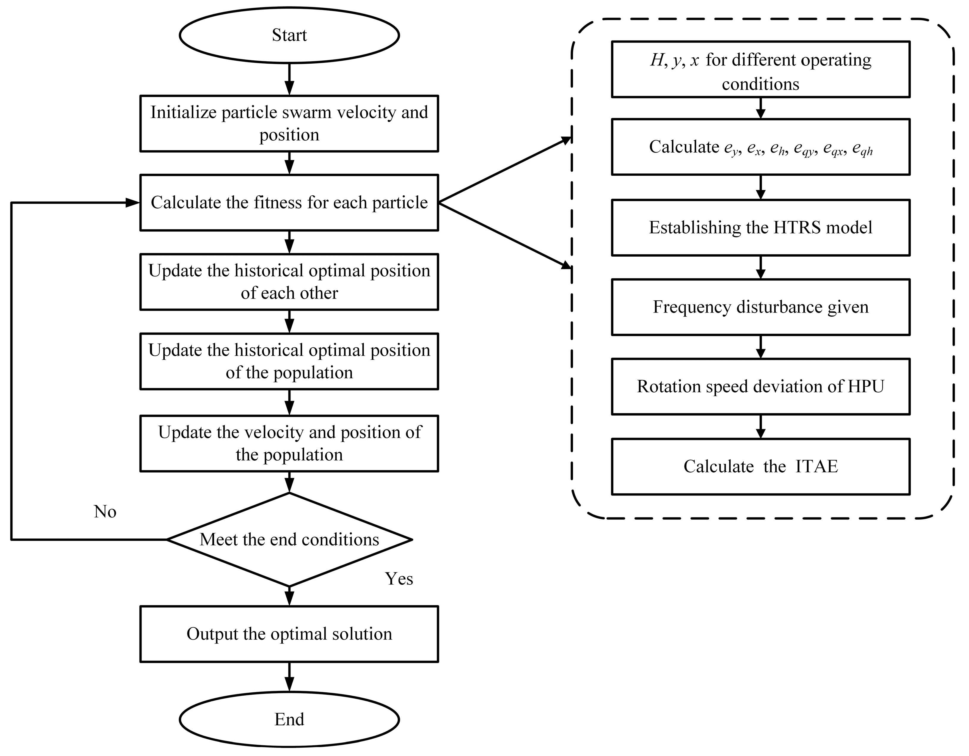
• Initialize particle swarm velocity and position. In the initial phase of the algorithm, velocities and positions are randomly assigned to particles in the solution space.
• Calculate the fitness of each particle. First, the transfer coefficients ($e_x$, $e_y$, $e_h$, $e_{qx}$, $e_{qy}$, $e_{qh}$) of the hydraulic turbine are calculated based on the state parameters ($y$, $H$, $x$) for the specified operating conditions. Based on this, the overall model of the HTRS corresponding to this operating condition is obtained. Then, the system is simulated at a given perturbation in frequency to obtain the rotational speed deviation response curve of the HPU. Finally, the ITAE is calculated by substituting the speed deviation into Equation (9) and used as the fitness of each particle to provide the reference for updating the particle velocity and position subsequently.
• Update the historical optimal position of each particle. If the current fitness is better than the historical record, replace the historical optimal position with the current optimal position.
• Update the historical optimal position of the population. If the particle’s $pbes{t}_i$ is better than the current $gbes{t}_i$, the latter is replaced by the former.
• Update the velocity and position of the population. The velocity and position of each particle are updated using Equation (8).
• Determine whether the end condition is met. If the number of iterations satisfies the maximum number of iterations, the algorithm will stop and output the optimal solution; otherwise, return to Step 2.

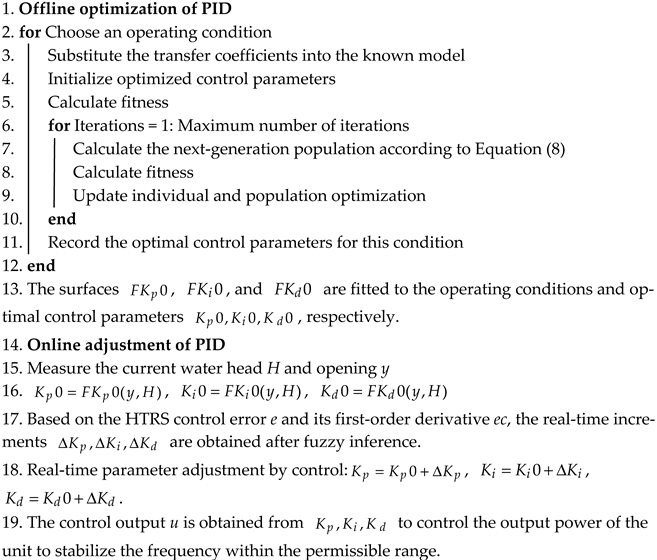
3.4. Adaptive Control of an HPU Based on the Particle Swarm Algorithm and Fuzzy PID

In this paper, the commonly used PID control and fuzzy control are combined to construct FPID that can adjust the PID parameters online, which integrates the advantages of human logical thoughts, language variables, and fuzzy reasoning of fuzzy theory, as well as the simple structure and high reliability of the traditional PID algorithm. On this basis, the initial parameters of FPID are optimized offline using the PSO algorithm, and a nonlinear relationship between the optimal initial parameters and operating conditions is established. By incorporating the fuzzy inference to adjust PID parameters online and PSO to optimize PID parameters offline, the PSO-FPID control strategy adapted to the variable operating conditions of the HPU is proposed, with the structure shown in Figure 6. In Figure 6, $r(t)$ is the given rotational speed of the HPU and $x(t)$ is the actual rotational speed.

The execution process of the PSO-FPID controller is described below. Firstly, the PSO algorithm is applied to determine the optimal initial control parameters $K_{p}0,K_{i}0,K_{d}0$ for the proportional, integral, and differential parts of the controller according to the current operating condition of the HPU (GVO $y$ and water head $H$). The process is offline, and the optimal initial values can be searched as soon as the operating condition and the objective function are determined. Secondly, the speed deviation and its change rate are regarded as the input of the fuzzy system, and the changes in the control parameters, $\Delta K_p,\Delta K_i,\Delta K_d$ are obtained after a series of fuzzy reasoning. Finally, the optimal initial PID parameters and their changes are summed up as the final control parameters $K_p,K_i,K_d$, which are shown in Equation (10). The control strategy consists of online optimization of PID by fuzzy inference and offline optimization of PID by PSO.

$$\left\{\begin{array}{l}{K}_p=K_{p}0+\Delta K_p\\ K_i=K_{i}0+\Delta K_i\\ K_d=K_{d}0+\Delta K_d\end{array}\right.$$

(10)

As the fuzzy inference does not take into account the change in the unit characteristics caused by the operating conditions, its control performance is greatly influenced by the initial values of the control parameters. In this paper, the PSO algorithm is introduced to optimize $K_{p}0,K_{i}0,K_{d}0$, which can largely reduce the deterioration of control performance caused by improper settings of $K_{p}0,K_{i}0,K_{d}0$. Based on the optimal initial values, the fuzzy inference system makes fine adjustments to the control parameters in real time during the dynamic process, which further improves the control performance of the controller. The PSO-FPID mathematical steps are shown in Algorithm 1.

Algorithm 1. PSO-FPID control of an HPU adapted to variable operating conditions

4. Numerical Experiments and Analysis

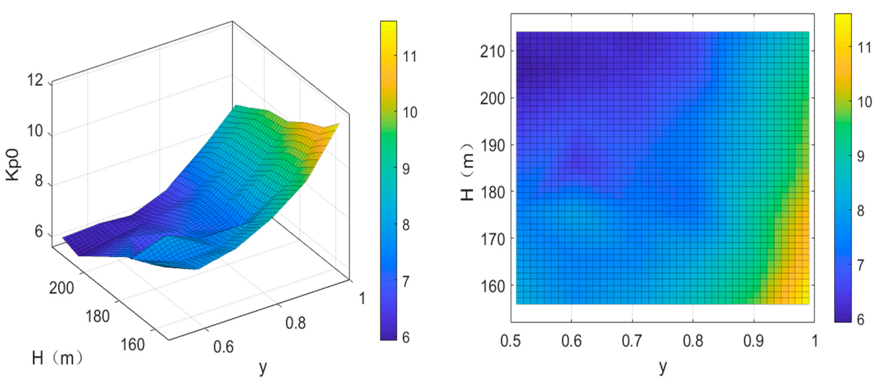
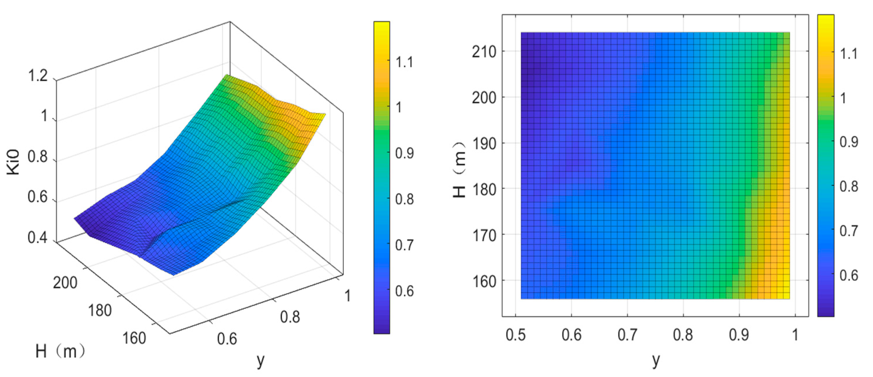
4.1. Results of PID Optimization Under Different Operating Conditions

In this section, the mathematical model that can reflect the change of operating conditions is built in the MATLAB R2022a/Simulink platform with the Francis HPU of an actual operating power station as the object. According to the range of water head and GVO during normal power generation of the HPU, 42 different operating conditions are selected for simulation to verify the performance of the designed PSO-FPID. These conditions are obtained by two-by-two combinations of different water heads (H = 155, 165, 175, 185, 195, 205, 215 m) and different GVOs (y = 0.5, 0.6, 0.7, 0.8, 0.9, 1.0). The parameters used for the HTRS in this paper are as follows: $T_y$ = 0.4594, $T_w$ = 0.8728, $T_a$ = 12.24, $e_g$ = 0.0864. The values of $e_y$, $e_x$, $e_h$, $e_{qy}$, $e_{qx}$, and $e_{qh}$ for each operating condition are given in [38]. The key parameters of PSO are set as follows (See Appendix A for more details): $w$ is set to 0.6, and $c_1,c_2$ are set to 1.4; the population size is set to 30; the maximum number of iterations is set to 30; and the lower limit of the optimization variables (PID control parameters) is set to 0.1, and the upper limit is set to 15. The $K_{p}0$, $K_{i}0$, and $K_{d}0$ of PSO-FPID are optimized under 42 operating conditions, and the results are shown in Figure 7, Figure 8 and Figure 9.

The 3-D surface in Figure 7 is plotted with the GVO as the x-axis, the water head as the y-axis, and $K_{p}0$ as the z-axis. The 3D surface in Figure 8 is plotted with the GVO as the x-axis, the water head as the y-axis, and $K_{i}0$ as the z-axis. The 3D surface in Figure 9 is plotted with the GVO as the x-axis, the water head as the y-axis, and $K_{d}0$ as the z-axis. It can be seen that the changes in $K_{p}0,K_{i}0,K_{d}0$ show nonlinear characteristics, all of which are positively related to y and negatively related to H. At a low water head, all three are more sensitive to changes of y; at a high water head, the changes tend to smooth out. For $K_{p}0$, as y increases, the dynamic response of the system is accelerated, and a larger $K_{p}0$ is needed to match the rapidly varying operating conditions. As H decreases, the system energy decreases and the control effect is compensated for by increasing $K_{p}0$. For $K_{i}0$, the value needs to be increased to ensure the regulation accuracy when the unit is running in the high load zone (y is large, H is small); when the unit is running in the low load zone (y is small, H is large), the value is decreased to avoid the saturation of the integration. For $K_{d}0$, as y increases, the discharge is large, and stronger differentiation is needed to suppress overshoot. As H decreases, the energy of the system decreases, and differential control needs to be enhanced to speed up the response.

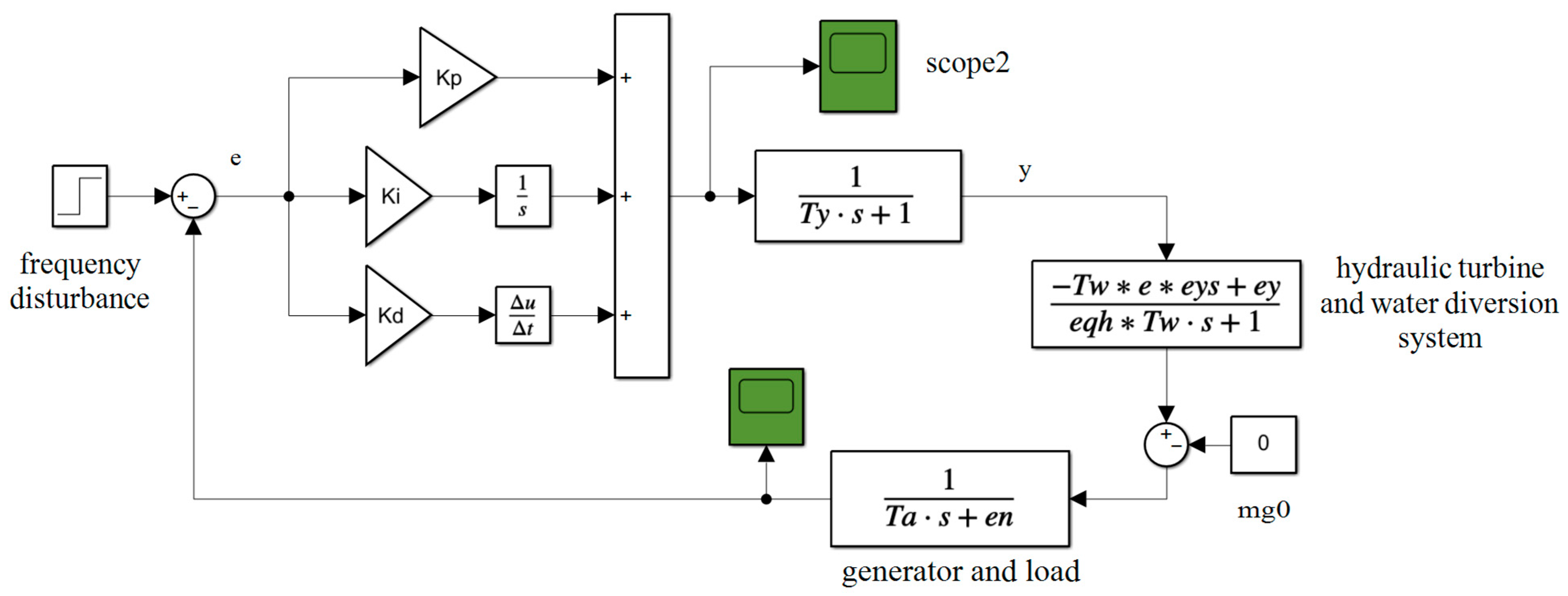
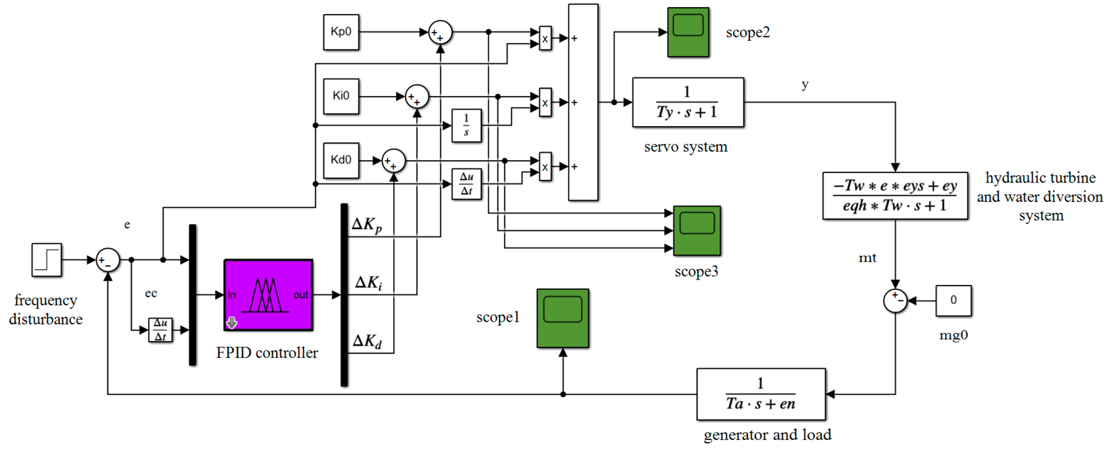
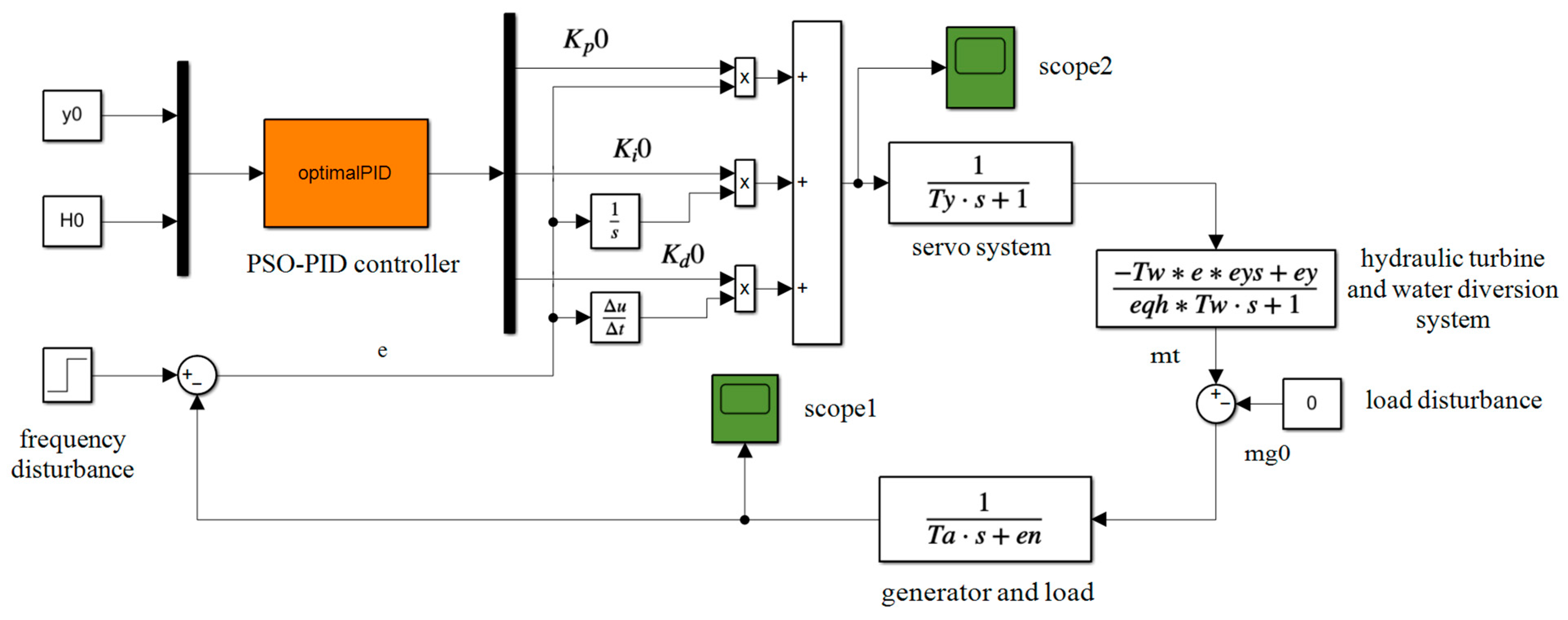
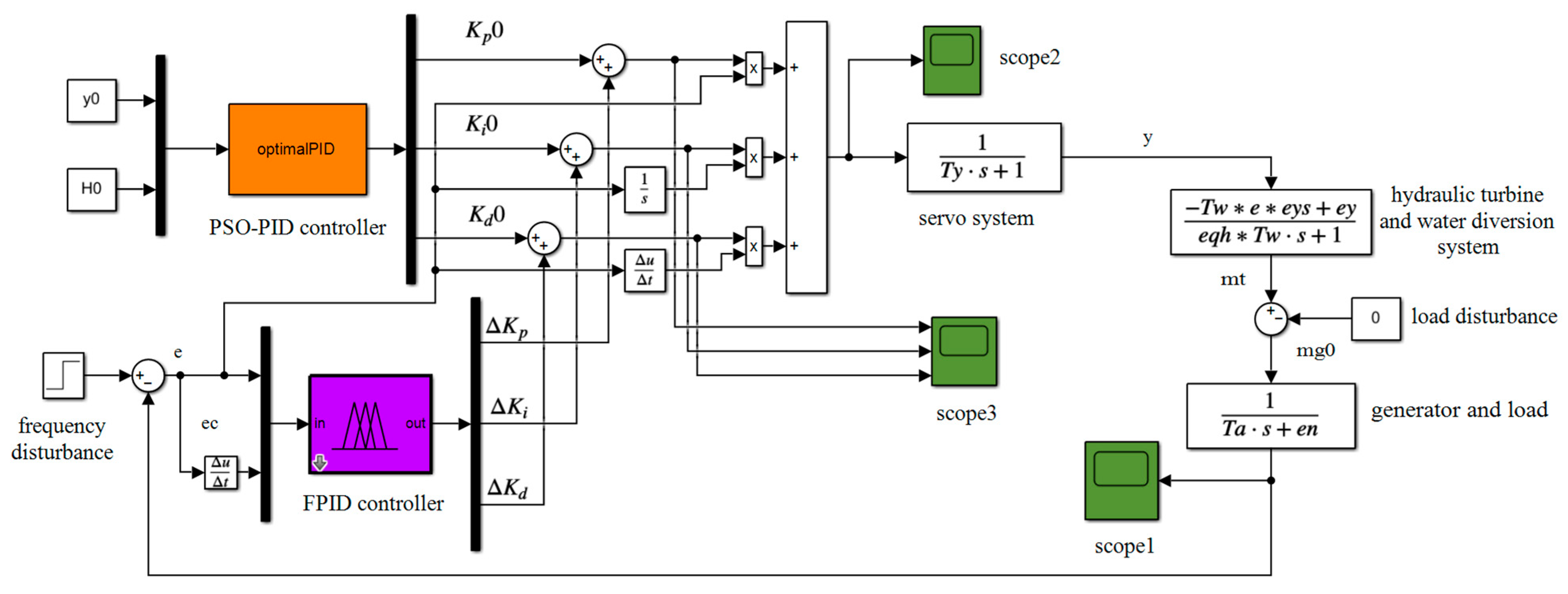
4.2. Simulation Models of Different Control Strategies

The simulation models of the HTRS under the four control strategies of PID, FPID, PSO-PID, and PSO-FPID are built in MATLAB/Simulink, as shown in Figure 10, Figure 11, Figure 12 and Figure 13.

The $K_p,K_i,K_d$ in Figure 10 are set to the actual control parameters 2, 0.2, and 0.2, respectively. The $K_{p}0,K_{i}0,K_{d}0$ in Figure 11 show the same results as the control parameter settings in Figure 10. The inputs of the “FPID controller” are the error e and its change rate ec for each operating condition of the HTRS, and the outputs are $\Delta K_p,\Delta K_i,\Delta K_d$ for the dynamic process. In Figure 12, the inputs of the “PSO-PID controller” are the GVO and water head for a given operating condition, and the outputs are the optimal initial parameters $K_{p}0,K_{i}0,K_{d}0$. Figure 13 shows that the HTRS model contains the control strategy proposed in this paper. In all four figures, the load disturbances are set to 0 and the frequency disturbances are +0.3% step disturbances.

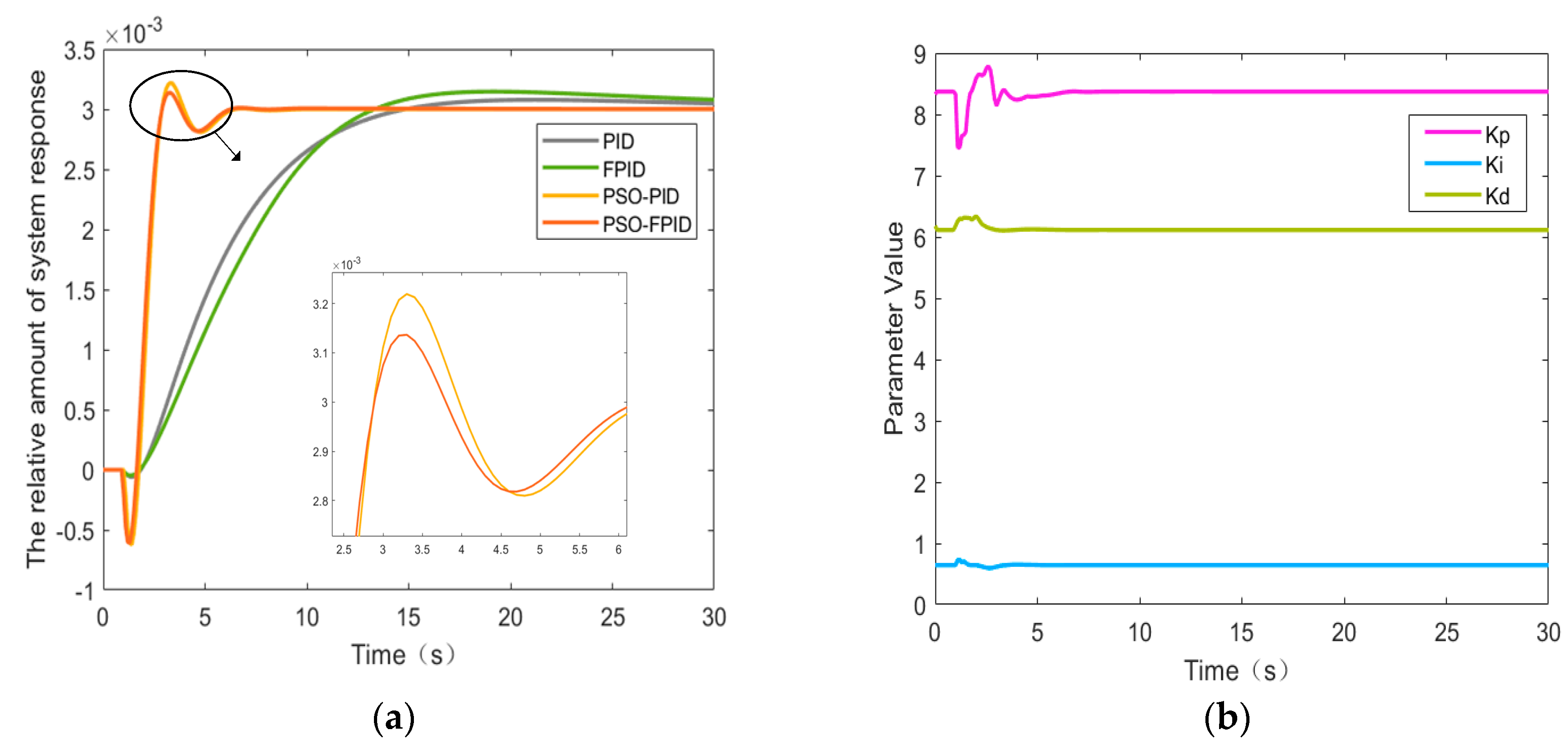
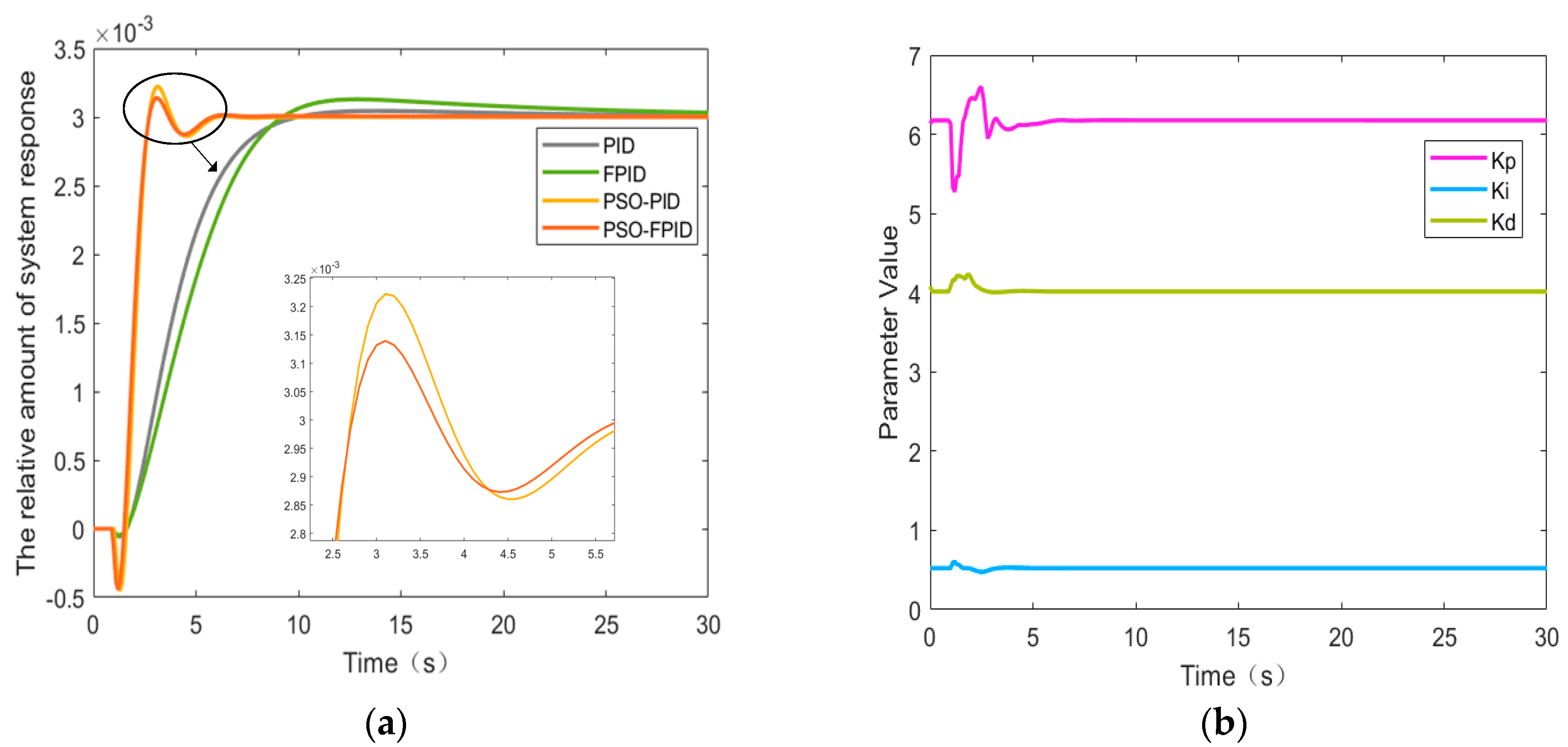
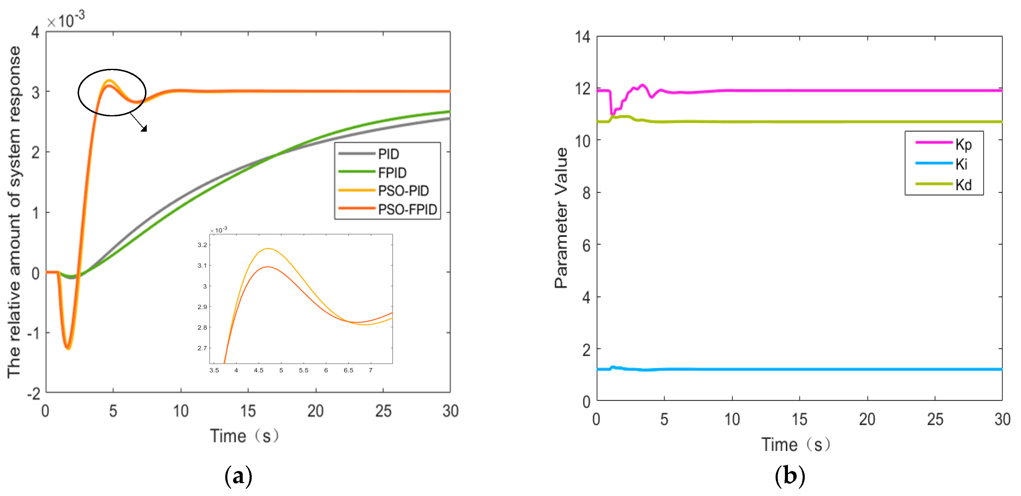
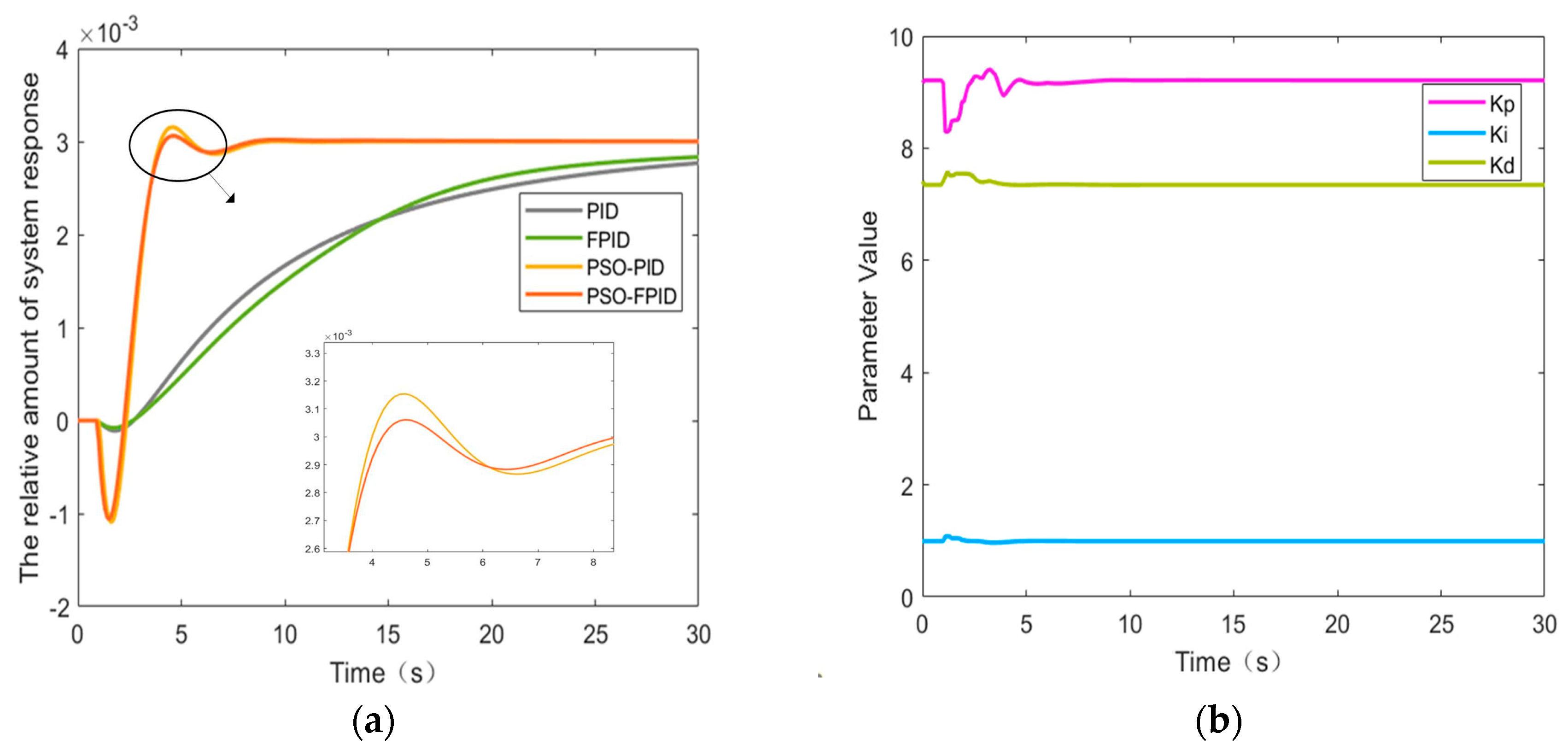
4.3. Performance Comparison and Analysis of Different Control Strategies

Numerical simulation of the transition process for the 42 conditions mentioned above is carried out using simulation models with different control strategies. The simulation time is 30 s, and the sampling time is 0.1 s. By disturbing the system under different control strategies with a step of +0.3% at a given frequency, the time-domain response waveforms of the system states can be obtained. They can be utilized to calculate the ITAE, adjust time, overshoot, reverse regulation, and number of oscillations of the system for 42 operating conditions. The results are shown in

Table 1. Performance indexes of each control strategy under 42 operating conditions.

Controller	H	y = 0.5					y = 0.6					y = 0.7
		ITAE	AT	OS	RR	NO	ITAE	AT	OS	RR	NO	ITAE	AT	OS	RR	NO
PID	155 m	0.0872	26.10	0.0261	0.0001	0.50	0.0961	15.90	0.0085	0.0001	0.00	0.1424	22.70	0.0000	0.0001	0.00
FPID		0.1128	29.00	0.0489	0.0000	0.50	0.1172	28.20	0.0274	0.0001	0.50	0.1334	17.60	0.0070	0.0001	0.00
PSO-PID		0.0088	4.80	0.0731	0.0006	0.50	0.0108	5.50	0.0531	0.0007	0.50	0.0130	6.10	0.0590	0.0008	0.50
PSO-FPID		0.0091	4.60	0.0455	0.0006	0.50	0.0117	5.20	0.0274	0.0007	0.50	0.0140	5.80	0.0296	0.0008	0.50
PID	165 m	0.0750	23.60	0.0250	0.0001	0.50	0.0810	14.60	0.0077	0.0001	0.00	0.1198	20.80	0.0000	0.0001	0.00
FPID		0.1026	29.00	0.0491	0.0000	0.50	0.1038	26.70	0.0286	0.0001	0.50	0.1172	16.00	0.0085	0.0001	0.00
PSO-PID		0.0088	4.50	0.0919	0.0007	0.50	0.0104	5.30	0.0733	0.0007	0.50	0.0123	5.90	0.0531	0.0008	0.50
PSO-FPID		0.0092	4.30	0.0602	0.0007	0.50	0.0110	5.10	0.0440	0.0007	0.50	0.0133	5.60	0.0224	0.0008	0.50
PID	175 m	0.0675	21.00	0.0235	0.0001	0.50	0.0715	13.30	0.0066	0.0001	0.00	0.1067	19.40	0.0000	0.0001	0.00
FPID		0.0934	28.60	0.0486	0.0000	0.50	0.0940	25.00	0.0290	0.0001	0.50	0.1045	14.80	0.0094	0.0001	0.00
PSO-PID		0.0080	4.50	0.0867	0.0006	0.50	0.0117	4.90	0.1928	0.0008	0.50	0.0118	5.70	0.0750	0.0008	0.50
PSO-FPID		0.0084	4.40	0.0571	0.0006	0.50	0.0116	5.70	0.1526	0.0008	1.00	0.0126	5.50	0.0419	0.0008	0.50
PID	185 m	0.0581	18.30	0.0217	0.0001	0.50	0.0606	12.40	0.0051	0.0001	0.00	0.0929	18.30	0.0000	0.0001	0.00
FPID		0.0851	26.90	0.0476	0.0001	0.50	0.0853	23.30	0.0288	0.0001	0.50	0.0940	13.80	0.0097	0.0001	0.00
PSO-PID		0.0165	6.40	0.6008	0.0007	1.00	0.0094	5.10	0.0415	0.0006	0.50	0.0114	5.60	0.0821	0.0007	0.50
PSO-FPID		0.0162	6.40	0.5695	0.0007	1.00	0.0105	4.80	0.0171	0.0006	0.50	0.0122	5.30	0.0493	0.0007	0.50
PID	195 m	0.0525	8.90	0.0194	0.0001	0.00	0.0544	11.50	0.0034	0.0001	0.00	0.0917	19.00	0.0000	0.0000	0.00
FPID		0.0775	25.20	0.0461	0.0001	0.50	0.0776	21.50	0.0281	0.0001	0.50	0.0837	14.20	0.0049	0.0000	0.00
PSO-PID		0.0145	6.10	0.5878	0.0007	1.00	0.0094	4.90	0.1058	0.0006	0.50	0.0067	4.00	0.1278	0.0003	0.50
PSO-FPID		0.0150	6.20	0.5577	0.0007	1.00	0.0100	4.80	0.0719	0.0006	0.50	0.0064	3.90	0.1163	0.0003	0.50
PID	205 m	0.0450	8.30	0.0173	0.0001	0.00	0.0462	10.80	0.0015	0.0001	0.00	0.0771	16.80	0.0000	0.0001	0.00
FPID		0.0708	23.50	0.0447	0.0001	0.50	0.0706	19.80	0.0270	0.0001	0.50	0.0770	12.20	0.0090	0.0001	0.00
PSO-PID		0.0071	4.30	0.0278	0.0004	0.50	0.0088	4.90	0.0640	0.0006	0.50	0.0104	5.30	0.0549	0.0007	0.50
PSO-FPID		0.0080	4.00	0.0097	0.0004	0.50	0.0096	4.70	0.0335	0.0006	0.50	0.0114	5.20	0.0228	0.0007	0.50
PID	215 m	0.0409	7.70	0.0149	0.0001	0.00	0.0426	10.20	0.0000	0.0001	0.00	0.0733	16.40	0.0000	0.0001	0.00
FPID		0.0647	21.90	0.0430	0.0000	0.50	0.0643	17.90	0.0257	0.0001	0.50	0.0700	11.50	0.0081	0.0001	0.00
PSO-PID		0.0069	4.30	0.0742	0.0005	0.50	0.0087	4.60	0.0993	0.0006	0.50	0.0100	5.30	0.0463	0.0006	0.50
PSO-FPID		0.0076	4.10	0.0466	0.0004	0.50	0.0093	4.60	0.0631	0.0006	0.50	0.0111	5.10	0.0155	0.0006	0.50
Controller	H	y = 0.8					y = 0.9					y = 1.0
		ITAE	AT	OS	RR	NO	ITAE	AT	OS	RR	NO	ITAE	AT	OS	RR	NO
PID	155 m	0.2193	29.00	0.0000	0.0001	0.00	0.3214	29.00	0.0000	0.0001	0.00	0.4523	29.00	0.0000	0.0001	0.00
FPID		0.2015	26.40	0.0000	0.0001	0.00	0.3009	29.00	0.0000	0.0001	0.00	0.4311	29.00	0.0000	0.0001	0.00
PSO-PID		0.0152	6.40	0.0605	0.0010	0.50	0.0173	7.00	0.0471	0.0010	0.50	0.0200	7.40	0.0608	0.0013	0.50
PSO-FPID		0.0161	6.20	0.0300	0.0009	0.50	0.0182	6.60	0.0192	0.0010	0.50	0.0202	7.10	0.0311	0.0012	0.50
PID	165 m	0.1896	29.00	0.0000	0.0001	0.00	0.2863	29.00	0.0000	0.0001	0.00	0.4155	29.00	0.0000	0.0001	0.00
FPID		0.1749	23.50	0.0000	0.0001	0.00	0.2692	29.00	0.0000	0.0001	0.00	0.3968	29.00	0.0000	0.0001	0.00
PSO-PID		0.0143	6.40	0.0464	0.0009	0.50	0.0164	6.80	0.0380	0.0010	0.50	0.0188	7.30	0.0433	0.0012	0.50
PSO-FPID		0.0155	6.00	0.0178	0.0009	0.50	0.0175	6.40	0.0101	0.0010	0.50	0.0196	6.90	0.0166	0.0011	0.50
PID	175 m	0.1683	28.50	0.0000	0.0001	0.00	0.2624	29.00	0.0000	0.0001	0.00	0.3894	29.00	0.0000	0.0001	0.00
FPID		0.1512	20.50	0.0000	0.0001	0.00	0.2429	29.00	0.0000	0.0001	0.00	0.3675	29.00	0.0000	0.0001	0.00
PSO-PID		0.0155	6.50	0.0669	0.0011	0.50	0.0158	6.70	0.0634	0.0010	0.50	0.0181	7.10	0.0486	0.0011	0.50
PSO-FPID		0.0169	6.20	0.0278	0.0010	0.50	0.0166	6.30	0.0330	0.0010	0.50	0.0188	6.80	0.0209	0.0011	0.50
PID	185 m	0.1513	27.60	0.0000	0.0001	0.00	0.2374	29.00	0.0000	0.0001	0.00	0.3613	29.00	0.0000	0.0001	0.00
FPID		0.1368	19.70	0.0000	0.0001	0.00	0.2211	29.00	0.0000	0.0001	0.00	0.3424	29.00	0.0000	0.0001	0.00
PSO-PID		0.0130	6.10	0.0346	0.0008	0.50	0.0151	6.50	0.0385	0.0009	0.50	0.0177	7.00	0.0316	0.0011	0.50
PSO-FPID		0.0143	5.70	0.0062	0.0008	0.50	0.0162	6.20	0.0099	0.0009	0.50	0.0187	6.70	0.0048	0.0011	0.50
PID	195 m	0.1399	26.60	0.0000	0.0001	0.00	0.2215	29.00	0.0000	0.0001	0.00	0.3425	29.00	0.0000	0.0001	0.00
FPID		0.1233	18.40	0.0000	0.0001	0.00	0.2029	29.00	0.0000	0.0001	0.00	0.3209	29.00	0.0000	0.0001	0.00
PSO-PID		0.0126	5.90	0.0635	0.0008	0.50	0.0146	6.40	0.0628	0.0009	0.50	0.0170	6.90	0.0527	0.0011	0.50
PSO-FPID		0.0135	5.70	0.0300	0.0008	0.50	0.0154	6.10	0.0310	0.0009	0.50	0.0177	6.60	0.0236	0.0011	0.50
PID	205 m	0.1267	25.90	0.0000	0.0001	0.00	0.2034	29.00	0.0000	0.0001	0.00	0.3209	29.00	0.0000	0.0001	0.00
FPID		0.1123	17.40	0.0000	0.0001	0.00	0.1876	29.00	0.0000	0.0001	0.00	0.3023	29.00	0.0000	0.0001	0.00
PSO-PID		0.0130	6.10	0.0346	0.0008	0.50	0.0143	6.30	0.0813	0.0009	0.50	0.0165	6.80	0.0413	0.0010	0.50
PSO-FPID		0.0143	5.70	0.0062	0.0008	0.50	0.0150	6.00	0.0475	0.0009	0.50	0.0175	6.40	0.0142	0.0010	0.50
PID	215 m	0.1198	25.40	0.0000	0.0001	0.00	0.1929	29.00	0.0000	0.0001	0.00	0.3069	29.00	0.0000	0.0001	0.00
FPID		0.1034	16.50	0.0000	0.0001	0.00	0.1748	29.00	0.0000	0.0001	0.00	0.2857	29.00	0.0000	0.0001	0.00
PSO-PID		0.0117	5.80	0.0408	0.0007	0.50	0.0136	6.20	0.0503	0.0009	0.50	0.0167	6.80	0.0513	0.0011	0.50
PSO-FPID		0.0130	5.40	0.0127	0.0007	0.50	0.0146	5.90	0.0202	0.0008	0.50	0.0176	6.50	0.0203	0.0011	0.50

Notes: AT, OS, RR and NO denote the adjust time (in s), the overshoot amount, the reverse regulation amount and the number of oscillations, respectively. Different colors indicate different performance indicators. The darker the color, the greater the value of the corresponding performance index, and vice versa.

. The average control performance of PSO-FPID is improved for the 42 operating conditions covered. The average adjust time of PSO-FPID is 16.60 s less than that of PID, 18.05 s less than that of FPID, and 0.23 s less than that of PSO-PID. The average overshoot of PSO-FPID is 6.13% higher than PID, 3.92% higher than FPID, and 2.96% lower than PSO-PID. The adjust time and the overshoot are contradictory. To satisfy the rapidity, when the adjust time is reduced significantly, an increase in the overshoot is inevitably induced. However, the overshoot does not exceed 30%, which is consistent with the operating conditions. In addition, the variation in PSO-FPID reverse regulation is very small compared to PID, FPID, and PSO-PID, which can be disregarded.

It can be seen from Table 1 that under 42 operating conditions, the amount of reverse regulation of FPID is slightly smaller than that of PID, while the amount of overshoot is slightly larger than that of PID. The ITAE and adjust time of FPID are better than that of PID only under some operating conditions. This reflects the limitations of FPID: its performance is significantly affected by the setting of $K_{p}0,K_{i}0,K_{d}0$ and lacks consideration of the global dynamic performance of the system. The regulation performance of the system may deteriorate if the initial control parameters are not properly selected. Therefore, it is necessary to optimize the initial values of FPID. The ITAE and adjust time of PSO-PID are substantially better than those of PID for each operating condition. The amount of overshoot, reverse regulation, and number of oscillations of PSO-PID are slightly poor compared to PID. The adjust time, overshoot, and reverse regulation of PSO-FPID are better than those of PSO-PID, except for the two operating conditions of H = 195, y = 0.5 and H = 175, y = 0.6.

The decrease rate of adjust time and the increase rate of overshoot of FPID compared to PID under 42 operating conditions are shown in Figure 14. The reduction rate of adjust time and increase rate of overshoot of PSO-PID compared to PID under 42 operating conditions are shown in Figure 15. The reduction rate of adjust time and the increase rate of overshoot for PSO-FPID compared to PSO-PID are shown in Figure 16. The sample values in Figure 14a, Figure 15a, Figure 16a represent indicators at different water heads. The black numbers in Figure 14b, black numbers in Figure 15b, and white numbers in Figure 16b indicate that the overshoot increase rate in this case has a large difference from the nearby cases.

As can be seen from Figure 14a, GVO is shown in the horizontal coordinate, and the adjust time reduction rate is shown in the vertical coordinate. At the same GVO, different adjust time reduction rates represent different water heads. When the GVO is 0.5, all of the adjust time reduction rates are negative and their distribution range is large, which indicates that the adjust time of FPID is longer than that of PID in small openings. As the GVO increases, the adjust time of FPID is less than or equal to that of PID. Figure 14b shows the overshoot increase rate under different GVOs and water heads. The effect of water heads on the overshoot increase rate is not significant. The general trend is that as the GVO increases, the increase rate of overshoot first decreases and then increases. When the GVO is 0.7, the increase rate of overshoot reaches the minimum value; when the GVO is 1.0, the overshoot increase reaches the maximum value. As a result, the performance of FPID is not always better than that of PID.

As can be seen from Figure 15a, the adjust time reduction rates are all positive, indicating that the adjust time of PSO-PID is shorter than that of PID under all operating conditions. The overshoot increase rates in Figure 15b are all positive, indicating that the overshoot of PSO-PID relative to PID increases under all operating conditions, but the increase amount is small. The maximum overshoot increase rate occurs when the GVO is 0.5 and the water head is 185 m. Therefore, PSO-PID has better performance compared to PID control.

As can be seen from Figure 16a, the adjust time reduction rate is mostly positive, indicating that PSO-FPID further reduces the adjust time concerning PSO-PID. The overshoot increase rates in Figure 16b are all negative, indicating that the PSO-FPID overshoot relative to the PSO-PID overshoot reduces under all operating conditions. The reduction of overshoot is greatest when the GVO is 0.6 and the water head is 174 m. Therefore, PSO-FPID has better performance compared to PSO-PID control. In summary, PSO-FPID control shows better overall performance under different operating conditions.

Finally, numerical simulations under typical operating conditions are carried out to further compare the difference between the dynamic adjust processes of different control strategies. The five operating conditions chosen are (1) H = 155 m, y = 0.5; (2) H = 215 m, y = 0.5; (3) H = 195 m, y = 0.7; (4) H = 155 m, y = 1.0; and (5) H = 215 m, y = 1.0. The response curves of the given frequency step perturbation and the dynamic change curves of the PSO-FPID parameters can be obtained through numerical simulation under different operating conditions and different control strategies. The results are shown in Figure 17, Figure 18, Figure 19, Figure 20 and Figure 21. In Figure 17 (H = 155 m, y = 0.5), the adjust time is 26.1 s for PID and 29 s for FPID. In Figure 18 (H = 215 m, y = 0.5), the adjust time is 7.7 s for PID and 21.9 s for FPID. Therefore, the dynamic quality of FPID is inferior to PID for these two boundary conditions. In Figure 19 (H = 195 m, y = 0.7), the adjust time of PID is 19 s and that of FPID is 14.2 s, and the dynamic quality of FPID is better than that of PID. The adjust times of PID and FPID in Figure 20 (H = 155 m, y = 1.0) and Figure 21 (H = 215 m, y = 1.0) are both 29 s, and the number of oscillations is also 0. The reverse regulation of FPID is slightly smaller than that of PID. Therefore, under these two conditions, the dynamic performance improvement effect of FPID compared to PID is not significant. The results show that FPID improves dynamic performance compared to PID only at the three boundary conditions of H = 195 m, y = 0.7, H = 155 m, y = 1.0, and H = 215 m, y = 1.0. From the frequency disturbance response curves of each condition, it can be seen that the control performance of both PSO-PID and PSO-FPID is better than that of PID and FPID due to their optimized control parameters. From the parameter changes of PSO-FPID, all three parameters are slightly adjusted in the dynamic process and finally reach a steady state. Compared to $K_p$, the adjustments of $K_i$ and $K_d$ are small and show a trend of first increasing and then decreasing, and finally reaching stability. The adjustment of $K_p$ tends to first decrease and then increase, and eventually decrease to stability.

Further, the performance indexes of different control strategies for frequency disturbance are calculated under five typical operating conditions, and the results are shown in

Table 2. Performance indexes of each control strategy under five typical operating conditions.

Operating Condition	Controller	Adjust Time (s)	Overshoot (%)	Reverse Regulation (%)	Number of Oscillations
H = 155 m y = 0.5	PID	26.100	2.610	0.006	0.500
	FPID	29.000	4.885	0.005	0.500
	PSO-PID	4.800	7.310	0.062	0.500
	PSO-FPID	4.600	4.550	0.061	0.500
H = 215 m y = 0.5	PID	7.700	1.489	0.006	0
	FPID	21.900	4.295	0.005	0.500
	PSO-PID	4.300	7.417	0.045	0.500
	PSO-FPID	4.100	4.656	0.044	0.500
H = 195 m y = 0.7	PID	19.000	0	0.001	0
	FPID	14.200	0.495	0.001	0
	PSO-PID	4.000	12.777	0.026	0.500
	PSO-FPID	3.900	11.632	0.026	0.500
H = 155 m y = 1.0	PID	29.000	0	0.009	0
	FPID	29.000	0	0.007	0
	PSO-PID	7.400	6.075	0.128	0.500
	PSO-FPID	7.100	3.108	0.125	0.500
H = 215 m y = 1.0	PID	29.000	0	0.011	0
	FPID	29.000	0	0.008	0
	PSO-PID	6.800	5.131	0.109	0.500
	PSO-FPID	6.500	2.031	0.106	0.500

. Combining the response curves of the above five typical operating conditions with the performance comparison of the controllers, it can be seen that the two indexes of overshoot and the number of oscillations under the PID control strategy are better than those of the other three control strategies. However, the adjust time of PID control is too long, and the dynamic process is unstable under some operating conditions, which must be avoided. The comprehensive regulation performance of FPID is not always better than that of PID, indicating that FPID has poor robustness. Compared to PID, PSO-PID significantly reduces the adjust time and improves the stability of the system. Although PSO-PID slightly increases the overshoot, reverse regulation, and number of oscillations, the increase is rather limited, indicating a better overall control performance. In addition, PSO-FPID further reduces the adjust time, overshoot, and reverse regulation based on PSO-PID. The response speed of the system is increased, and the stability is further improved.

5. Conclusions

To improve the control performance of the traditional fixed-parameter PID under variable operating conditions, a PSO-FPID controller is proposed for the HPU, combining the online adjustment of fuzzy inference and the offline optimization of PSO. From the perspectives of performance indexes and response curves, PSO-FPID is compared with PID, FPID, PSO-PID, and PSO-FPID under 42 operating conditions. The results show that the control performance of PSO-FPID is improved under most operating conditions. The average adjust time of PSO-FPID is 16.60 s less than that of PID, 18.05 s less than that of FPID, and 0.23 s less than that of PSO-PID. The average overshoot of PSO-FPID is higher than that of PID and FPID, which is due to the fact that the adjust time and overshoot are generally contradictory. However, none of the overshoots in this paper exceeds 30%, which satisfies the engineering requirements. In addition, the reverse regulation variation in PSO-FPID is very small compared to PID, FPID, and PSO-PID, which can be disregarded.

In addition to the improvement in the performance index, the proposed control strategy has a broad application prospect. Without changing the original control structure, the parameters of PID are optimized in real time with only less computational cost, which can be easily applied to real power plants. By reducing the dynamic process adjustment time of the HPU, the maintenance cost due to guide vane wear can be reduced while increasing auxiliary service revenue.

In future work, consideration needs to be given to integrating complex hydraulic and power system models into the optimized control and operation of HPUs to meet the real-world control needs of more complex scenarios.

References

- Li, Y.; Tong, Z.; Zhang, J.; Liu, D.; Yue, X.; Mahmud, M.A. Operational Characteristics Assessment of a Wind–Solar–Hydro Hybrid Power System with Regulating Hydropower. Water 2023, 15, 4051. [Google Scholar] [CrossRef]
- Yang, W.; Norrlund, P.; Saarinen, L.; Witt, A.; Smith, B.; Yang, J.; Lundin, U. Burden on hydropower units for short-term balancing of renewable power systems. Nat. Commun. 2018, 9, 2633. [Google Scholar] [CrossRef] [PubMed]
- Pan, J.-S.; Yue, L.; Chu, S.-C.; Hu, P.; Yan, B.; Yang, H. Binary bamboo forest growth optimization algorithm for feature selection problem. Entropy 2023, 25, 314. [Google Scholar] [CrossRef] [PubMed]
- Illias, H.; Nurjannah, N.; Mokhlis, H. Optimization of Automatic Generation Control Performance for Power System of Two-Area based on Genetic Algorithm-Particle Swarm Optimization. In Proceedings of the 2024 IEEE 4th International Conference in Power Engineering Applications (ICPEA), Pulau Pinang, Malaysia, 4–5 March 2024. [Google Scholar]
- Ding, T.; Chang, L.; Li, C.; Feng, C.; Zhang, N. A mixed-strategy-based whale optimization algorithm for parameter identification of hydraulic turbine governing systems with a delayed water hammer effect. Energies 2018, 11, 2367. [Google Scholar] [CrossRef]
- Lei, G.; Chang, X.; Tianhang, Y.; Tuerxun, W. An Improved Mayfly Optimization Algorithm Based on Median Position and Its Application in the Optimization of PID Parameters of Hydro-Turbine Governor. IEEE Access 2022, 10, 36335–36349. [Google Scholar] [CrossRef]
- Da Silva, C.S.; Da Silva, N.J.; Florindo, A.D.; De Medeiros, R.L.; Silva, L.E.; De Lucena, V.F. Experimental Implementation of Hydraulic Turbine Dynamics and a Fractional Order Speed Governor Controller on a Small-Scale Power System. IEEE Access 2024, 12, 40480–40495. [Google Scholar] [CrossRef]
- Köse, I.H.; Danayiyen, Y.; Çavdar, B. Fractional order PID controller design for hydroelectric power plant model with PSO, GWO and MA optimization algorithms. In Proceedings of the 2023 Innovations in Intelligent Systems and Applications Conference (ASYU), Sivas, Turkey, 11–13 October 2023. [Google Scholar]
- Rajagopal, K.; Jahanshahi, H.; Jafari, S.; Weldegiorgis, R.; Karthikeyan, A.; Duraisamy, P. Coexisting attractors in a fractional order hydro turbine governing system and fuzzy PID based chaos control. Asian J. Control 2021, 23, 894–907. [Google Scholar] [CrossRef]
- Piraisoodi, T.; Maria Siluvairaj, W.I.; Kappuva, M.A.K. Multi-objective robust fuzzy fractional order proportional–integral–derivative controller design for nonlinear hydraulic turbine governing system using evolutionary computation techniques. Expert Syst. 2019, 36, e12366. [Google Scholar] [CrossRef]
- Gheisarnejad, M. An effective hybrid harmony search and cuckoo optimization algorithm based fuzzy PID controller for load frequency control. Appl. Soft Comput. 2018, 65, 121–138. [Google Scholar] [CrossRef]
- Jovanović, R.Ž.; Božić, I.O. Feedforward neural network and ANFIS-based approaches to forecasting the off-cam energy characteristics of Kaplan turbine. Neural Comput. Appl. 2018, 30, 2569–2579. [Google Scholar] [CrossRef]
- Weldcherkos, T.; Salau, A.O.; Ashagrie, A. Modeling and design of an automatic generation control for hydropower plants using Neuro-Fuzzy controller. Energy Rep. 2021, 7, 6626–6637. [Google Scholar] [CrossRef]
- Jiang, X.; Chen, X.; Wang, Z. Research on modeling and control strategy of hydraulic turbine governing system based on improved genetic algorithm. IOP Conf. Ser. Earth Environ. Sci. 2018, 774, 012136. [Google Scholar] [CrossRef]
- Shi, K.; Wang, B.; Chen, H. Fuzzy generalised predictive control for a fractional-order nonlinear hydro-turbine regulating system. IET Renew. Power Gener. 2018, 12, 1708–1713. [Google Scholar] [CrossRef]
- Ma, T.; Wang, B.; Zhang, Z.; Yang, Y. A Takagi-Sugeno fuzzy-model-based finite-time H-infinity control for a hydraulic turbine governing system with time delay. Int. J. Electr. Power Energy Syst. 2021, 132, 107152. [Google Scholar] [CrossRef]
- Tian, Y.; Wang, B.; Chen, P.; Yang, Y. Finite-time Takagi–Sugeno fuzzy controller design for hydraulic turbine governing systems with mechanical time delays. Renew. Energy 2021, 173, 614–624. [Google Scholar] [CrossRef]
- Jiang, X.P.; Wang, Z.T.; Zhu, H.; Wang, W.S. Hydraulic turbine system identification and predictive control based on GASA-BPNN. International. J. Miner. Metall. Mater. 2021, 28, 1240–1247. [Google Scholar]
- Yu, P.; Yu, Y.; Ren, Z.; Wu, C.; Xu, Y. Research on speed regulation system of water turbine generator unit based on PID neural network. IOP Conf. Ser. Earth Environ. Sci. 2020, 525, 012101. [Google Scholar] [CrossRef]
- Zeng, Y.; Hussein, Z.A.; Chyad, M.H.; Farhadi, A.; Yu, J.; Rahbarimagham, H. Integrating type-2 fuzzy logic controllers with digital twin and neural networks for advanced hydropower system management. Sci. Rep. 2025, 15, 5140. [Google Scholar] [CrossRef]
- Liu, D.; Zhang, J.; Lu, X.; Li, C.; Malik, O.P. Model-free adaptive optimal control for fast and safe start-up of pumped storage hydropower units. J. Energy Storage 2024, 87, 111345. [Google Scholar] [CrossRef]
- Chen, J.; Liu, S.; Wang, Y.; Hu, W.; Zou, Y.; Zheng, Y.; Xiao, Z. Generalized predictive control application scheme for nonlinear hydro-turbine regulation system: Based on a precise novel control structure. Energy 2024, 296, 130916. [Google Scholar] [CrossRef]
- Dao, F.; Zou, Y.; Qian, J.; Zeng, Y. Design of a novel state-feedback robust sliding-mode controller for a hydraulic turbine governing system. Sci. Rep. 2024, 14, 29083. [Google Scholar] [CrossRef] [PubMed]
- Chen, J.; Zeng, Q.; Zou, Y.; Li, S.; Zheng, Y.; Liu, D.; Xiao, Z. Intelligent robust control for nonlinear complex hydro-turbine regulation system based on a novel state space equation and dynamic feedback linearization. Energy 2024, 302, 131798. [Google Scholar] [CrossRef]
- Wang, C.; Wang, D.-K.; Zhang, J.-M. Experimental study on the optimal strategy for power regulation of governing system of hydropower station. Water 2021, 13, 421. [Google Scholar] [CrossRef]
- Zeng, Y.; Yu, S.; Dao, F.; Li, X.; Xu, Y.; Qian, J. Hamiltonian Additional Damping Control for Suppressing Power Oscillation Induced by Draft Tube Pressure Fluctuation. Water 2023, 15, 1479. [Google Scholar] [CrossRef]
- Chen, J.; He, G.; Wang, Y.; Zheng, Y.; Xiao, Z. Adaptive PID Control for Hydraulic Turbine Regulation Systems Based on INGWO and BPNN. Prot. Control Mod. Power Syst. 2024, 9, 126–146. [Google Scholar] [CrossRef]
- Zhao, W.; Shi, T.; Wang, L.; Cao, Q.; Zhang, H. An adaptive hybrid atom search optimization with particle swarm optimization and its application to optimal no-load PID design of hydro-turbine governor. J. Comput. Des. Eng. 2021, 8, 1204–1233. [Google Scholar] [CrossRef]
- Lei, G. Application of improved PID control technology in hydraulic turbine governing systems. In Proceedings of the 2017 3rd International Conference on Control, Automation and Robotics (ICCAR), Nagoya, Japan, 22–24 April 2017. [Google Scholar]
- Jiang, X.P.; Zhu, H.; Wang, W.S.; Wang, Z.W.; Luo, Y.Y. Research on optimization of hydraulic turbine governor based on PSO algorithm. IOP Conf. Ser. Earth Environ. Sci. 2018, 163, 012098. [Google Scholar] [CrossRef]
- Liu, D.; Li, C.; Malik, O. Nonlinear modeling and multi-scale damping characteristics of hydro-turbine regulation systems under complex variable hydraulic and electrical network structures. Appl. Energy 2021, 293, 116949. [Google Scholar] [CrossRef]
- Liu, D.; Li, C.; Tan, X.; Lu, X.; Malik, O.P. Damping characteristics analysis of hydropower units under full operating conditions and control parameters: Accurate quantitative evaluation based on refined models. Appl. Energy 2021, 292, 116881. [Google Scholar] [CrossRef]
- Wang, C.; Li, D.H.; Zhang, H.L.; Ma, P.; Li, X.K.; Zhang, S.H.; Dong, Y.C. Prescribed performance sliding mode control for the bursting oscillation of a fractional-order hydro-turbine governing system based on time-varying tangent barrier Lyapunov function. Appl. Energy 2024, 356, 122414. [Google Scholar] [CrossRef]
- Wu, X.; Xu, Y.; Liu, J.; Lv, C.; Zhou, J.; Zhang, Q. Characteristics analysis and fuzzy fractional-order PID parameter optimization for primary frequency modulation of a pumped storage unit based on a multi-objective gravitational search algorithm. Energies 2019, 13, 137. [Google Scholar] [CrossRef]
- Barakat, M. Optimal design of fuzzy-PID controller for automatic generation control of multi-source interconnected power system. Neural Comput. Appl. 2022, 34, 18859–18880. [Google Scholar] [CrossRef]
- Liu, D.; Xiao, Z.; Li, H.; Liu, D.; Hu, X.; Malik, O.P. Accurate parameter estimation of a hydro-turbine regulation system using adaptive fuzzy particle swarm optimization. Energies 2019, 12, 3903. [Google Scholar] [CrossRef]
- Gong, X. Optimization of the power generation control process of hydraulic turbine set based on the improved BFO-PSO algorithm. J. Coast. Res. 2019, 94, 227–231. [Google Scholar] [CrossRef]
- Liu, D.; Wang, X.; Peng, Y.; Zhang, H.; Xiao, Z.; Han, X.; Malik, O.P. Stability analysis of hydropower units under full operating conditions considering turbine nonlinearity. Renew. Energy 2020, 154, 723–742. [Google Scholar] [CrossRef]