Article

Advancing Digital Image-Based Recognition of Soil Water Content: A Case Study in Bailu Highland, Shaanxi Province, China

1
Key Laboratory of Highway Construction Technology and Equipment of the Ministry of Education, Chang’an University, Xi’an 710064, China
2
State Key Laboratory of Resources and Environmental Information System, Institute of Geographic Sciences and Natural Resources Research, Chinese Academy of Sciences, Beijing 100101, China
3
School of Geological Engineering and Geomatics, Chang’an University, Xi’an 710064, China
4
China Construction First Group Corporation Limited, Xi’an 710075, China
*
Author to whom correspondence should be addressed.
Water 2024, 16(8), 1133; https://doi.org/10.3390/w16081133
Submission received: 5 March 2024 / Revised: 8 April 2024 / Accepted: 9 April 2024 / Published: 16 April 2024
(This article belongs to the Special Issue Research on Soil Moisture and Irrigation)

Abstract

:
Soil water content (SWC) plays a vital role in agricultural management, geotechnical engineering, hydrological modeling, and climate research. Image-based SWC recognition methods show great potential compared to traditional methods. However, their accuracy and efficiency limitations hinder wide application due to their status as a nascent approach. To address this, we design the LG-SWC-R3 model based on an attention mechanism to leverage its powerful learning capabilities. To enhance efficiency, we propose a simple yet effective encoder–decoder architecture (PVP-Transformer-ED) designed on the principle of eliminating redundant spatial information from images. This architecture involves masking a high proportion of soil images and predicting the original image from the unmasked area to aid the PVP-Transformer-ED in understanding the spatial information correlation of the soil image. Subsequently, we fine-tune the SWC recognition model on the pre-trained encoder of the PVP-Transformer-ED. Extensive experimental results demonstrate the excellent performance of our designed model (R2 = 0.950, RMSE = 1.351%, MAPE = 0.081, MAE = 1.369%), surpassing traditional models. Although this method involves processing only a small fraction of original image pixels (approximately 25%), which may impact model performance, it significantly reduces training time while maintaining model error within an acceptable range. Our study provides valuable references and insights for the popularization and application of image-based SWC recognition methods.

1. Introduction

Soil, as a complex natural resource, plays a crucial role under the integrated influence of water and human factors [1]. Water, an essential element in various forms and compositions, gives rise to intricate mechanisms and pathways that significantly influence the soil environment at multiple levels [2,3]. In the field of agriculture, soil water content (SWC) is vital for plant growth and development [4]. Adequate water supply at different growth stages is essential for any crop, as both too much and too little water can negatively impact crop yield and quality [5]. Accurately measuring SWC and distribution can assist farmers in scientifically scheduling irrigation, efficiently utilizing water resources, and avoiding issues such as soil salinization and water depth exceeding root zones caused by excessive irrigation [6]. In geotechnical engineering, changes in SWC significantly influence soil mechanical properties, permeability, and stability [7,8]. Even minor variations in SWC can lead to significant changes in soil strength, compressibility, and water conductivity, posing potential threats to the stability and safety of engineering structures [9]. Therefore, the accurate estimation and monitoring of soil water conditions are of paramount importance for geotechnical engineering design and construction. This can help engineers assess soil engineering properties and take appropriate measures to ensure the stability and safety of engineering projects [10]. Additionally, dynamic SWC data play a crucial role in disaster prevention and response. Monitoring SWC levels can serve as a precursor signal for geological disasters (such as landslides, debris flows), providing timely alerts and warnings [11]. In the fields of climate and water resources management, understanding the distribution and changes in SWC is critical for predicting and evaluating the risks of extreme weather events such as droughts and floods [12]. In summary, in-depth research and real-time monitoring of SWC are not only essential for the sustainable development of agricultural production and the safety of geotechnical engineering but also for disaster prevention and hydrological assessments.
There are various methods available for measuring SWC, which can be broadly classified into direct and indirect methods [13]. Direct methods include the oven-drying method [14]. Due to the high accuracy of this method, its results are usually considered as standard values. However, despite the high precision of these methods, they are time-consuming and destructive, thereby facing certain limitations in practical applications. In contrast, indirect methods include neutron moisture probe (NMP), resistance method (ERM), time domain reflectometry (TDR), frequency domain reflectometry (FDR), gamma-ray attenuation method (GRA), and remote sensing methods [3]. NMP and GRA methods exhibit high accuracy and response speed, but due to their involvement with radioactive elements, potential risks to human health and the environment may exist [15]. Other sensors (such as ERM, TDR, and FDR) require good soil contact, thus generating significant impact on measurement results in soils with cracks and voids [16]. Remote sensing methods, although capable of providing extensive data, are greatly influenced by climate and soil surface vegetation cover, and are only suitable for shallow soil layers [17]. Despite the availability of these methods, the widespread implementation of non-destructive SWC monitoring remains challenging due to their inherent limitations.
The machine learning-based methods using digital image analysis have been widely applied as a non-contact and on-site indirect measurement approach in studying soil properties, such as the hydraulic conductivity of soils [18], soil roughness [19], soil type [20], soil texture [21], soil bulk density [22], and total soil nitrogen content [23]. Many studies have focused on utilizing soil surface images to estimate SWC [13,24]. This is because the presence of water causes various changes in the spectrum of incident light around soil particles, including scattering, refraction, reflection, and absorption, which can be visually captured in a digital image taken by a camera [13]. Meanwhile, as the water content increases, the spectral reflectance of the soil decreases, and the soil image information typically becomes darker. Therefore, the distinct image information differences between dry and wet soil serve as the basis for image-based SWC prediction techniques [25,26]. Devices such as spectrometers, multispectral cameras, and thermal cameras can provide more spectral information for SWC prediction [27,28], but due to their high cost and complex operation, they are primarily used for scientific research. In contrast, digital cameras, with their relatively lower cost, offer a convenient way to indirectly assess SWC [29], attracting significant attention in the academic community. Previous research has concentrated on the real-time assessment of SWC variations by monitoring changes in soil image information. For instance, ref. [30] pioneered the utilization of Linear Regression to predict moisture from soil images in the RGB and HSV color spaces. Subsequently, notable research endeavors emerged: ref. [29] employed a multilayer perceptron (MLP) artificial neural network to recognize the moisture content of tropical soils taken by digital cameras. Ref. [31] opted for a simple linear regression model to recognize soil moisture between the saturation (S) and value (V) of soil images in the HSV color space. More recently, ref. [32] also utilized soil images captured by digital cameras to recognize SWC by constructing traditional machine learning models using features extracted from different color spaces in the images. Ref. [33] employed AlexNet (convolutional neural network) to build a classification model for predicting SWC based on soil surface images. These studies have shown that SWC recognition models based on soil images can rapidly, non-destructively, and conveniently measure SWC. However, as an emerging technology, there are still some important topics that require further discussion and research, which will be outlined in the following sections to address the current limitations in research.
1.
There is a need for more effective image-based SWC recognition regression methods. Previous studies have primarily utilized simple traditional machine learning models such as linear models [31], polynomial models [25], exponential models [34], and basic deep learning models [29,33]. However, research has shown that the response of soil image information to changes in SWC is not a straightforward relationship [13,31]. Simple models can lead to poor accuracy and stability in recognition, failing to meet application demands. Therefore, more effective regression models are needed to learn the complex patterns and feature representations in soil images, enhancing the accuracy and stability of SWC recognition regression.
2.
The high demand for computational resources has increased the threshold for application, limiting the potential for widespread use. Previous research has primarily focused on selecting useful input variables, such as mean and variance in the statistical color space of soil images [30,31,32,33]. However, selecting variables to represent the entire image may lead to the loss of valuable information within the image. As a viable alternative, many current studies choose to input all pixels of the entire image into the model without variable selection [32,33]. However, the computational and time costs for handling large amounts of data increase the usage threshold, requiring more expensive computational resources. This poses a challenge in resource-constrained environments. One way to address this issue is to develop more efficient algorithms and technologies to reduce computational and time costs, thus lowering the application threshold and increasing the potential for widespread use.
3.
Highly redundant spatial information in soil images. Highly redundant spatial information exists in traditional natural images [35,36]. However, soil images mainly consist of a significantly larger proportion of soil regions and a smaller proportion of non-soil areas (porous areas, mineral composition areas), where the redundant spatial information between these regions is more pronounced and highly similar compared to natural images. Yet, research on reducing the spatial redundancy in soil images to prevent the model from merely focusing on the low-level statistical distribution of images and truly understanding soil image characteristics is very limited.
To further propel the practical applications of image-based SWC recognition in relevant fields, this paper, leveraging the aforementioned limitations, establishes two key objectives. Firstly, to develop SWC models with superior performance compared to traditional models. Secondly, assuming the high redundancy of information in soil images and less pixel information can substitute the entire image, we aim to reduce the demand for computational resources by this hypothesis. Hence, the main contributions of this study are as follows:
1.
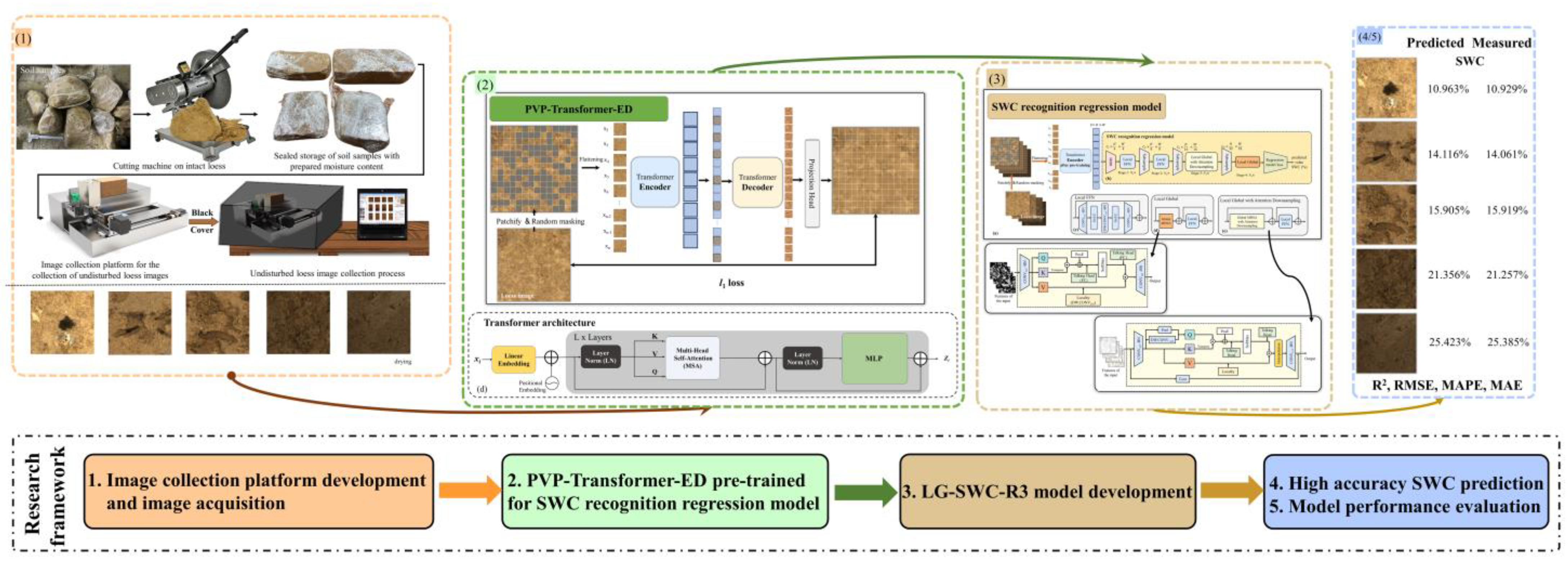
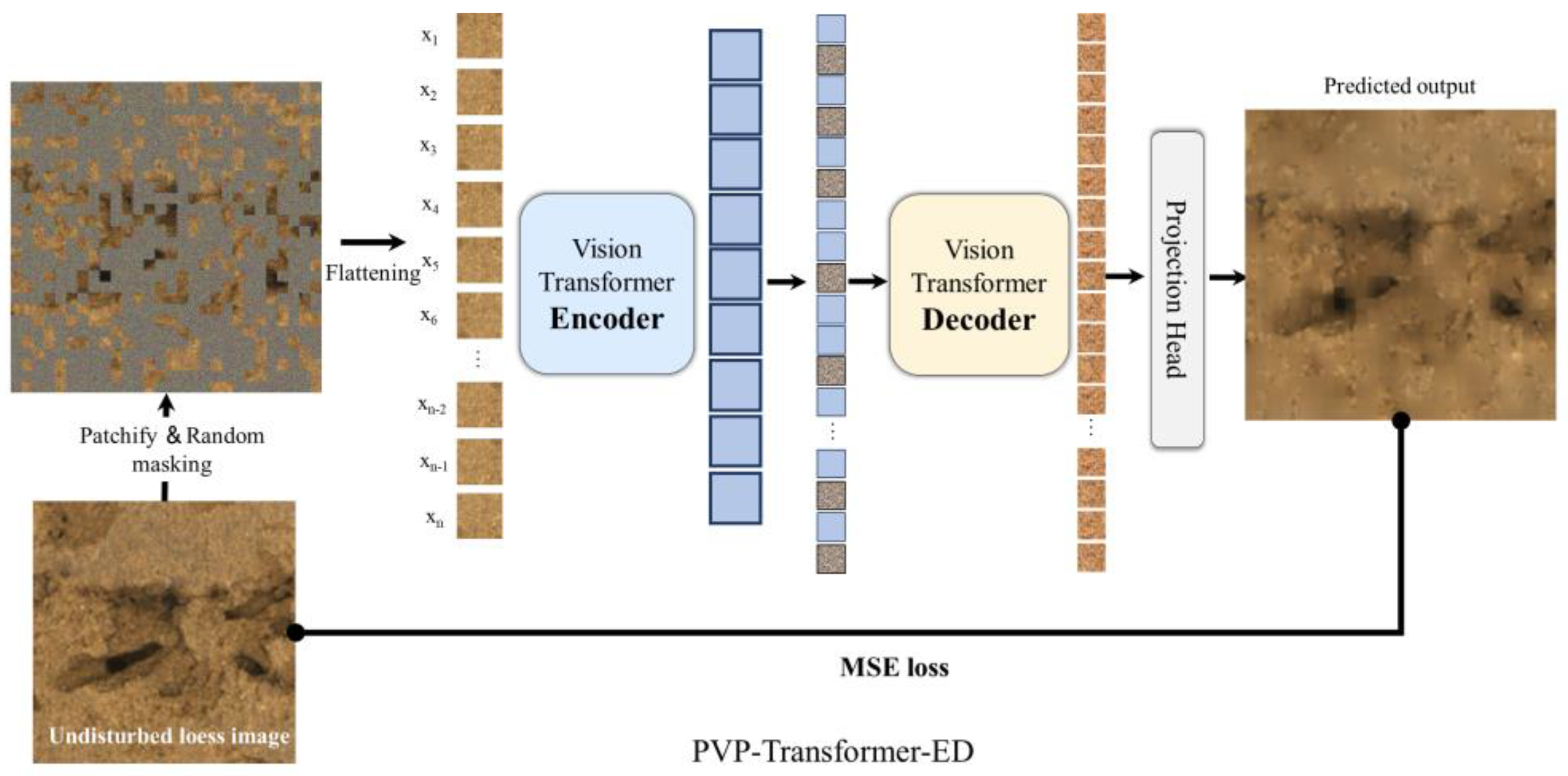
To reduce the demand for computational resources, we designed the PVP-Transformer-ED from the perspective of reducing spatial redundancy in soil images. Its aim is to randomly mask patches from the input image, reconstruct missing patches in pixel space to learn more complex patterns and feature representations in soil images, and then fine-tune the pretrained PVP-Transformer-ED on the regression model. It enables the SWC model to identify SWC with minimal input patches, reducing the recognition time by 50% or more. Additionally, it helps reduce memory consumption, thus providing the potential to extend the PVP-Transformer-ED to more complex large models and enhance generalization.
2.
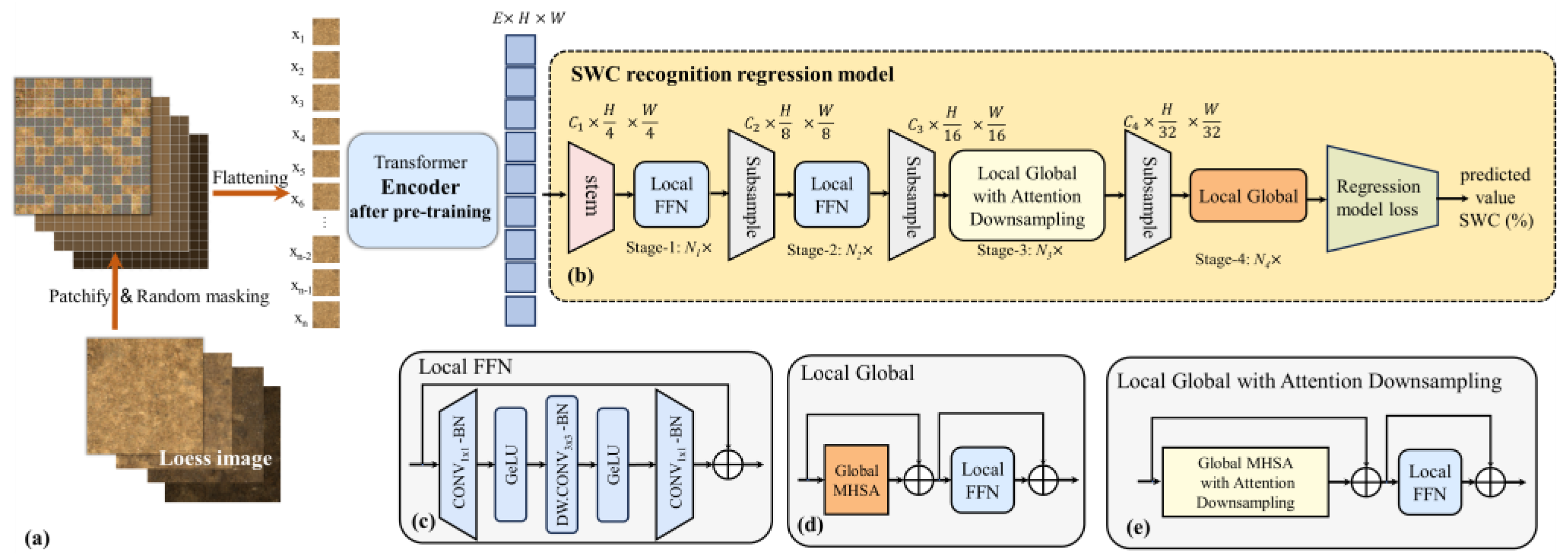
We designed the LG-SWC-R3 model based on the concept of local information and global perception to effectively capture the intricate relationship between SWC and image features. Experimental results have demonstrated that this model outperforms the aforementioned SWC recognition models across different evaluation metrics.
3.
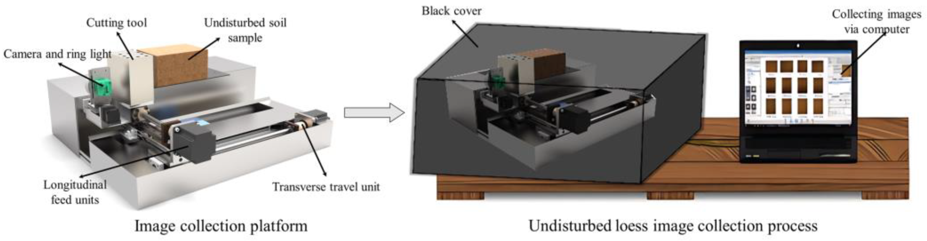
We developed an automatic image acquisition platform for constructing the undisturbed loess dataset and established the Bailu highland soil dataset based on this platform. This hardware and dataset support pave the way for future research endeavors.

2. Materials and Methods

The research framework is illustrated in Figure 1. Firstly, soil samples from Bailu highland were collected, and soil images with varying moisture levels were collected using the developed soil image acquisition platform for training and testing the moisture recognition model. Subsequently, a simple, effective, and scalable encoder–decoder architecture known as the Patch-based Visual Perception Encoder–Decoder Architecture based Transformer (PVP-Transformer-ED) was pretrained to endow certain regions within the soil images with the ability to represent the entire image. Building on the concept of local information and global perception, a local global SWC recognition regression model (LG-SWC-R3 model) was designed. We will describe each of them in this section.

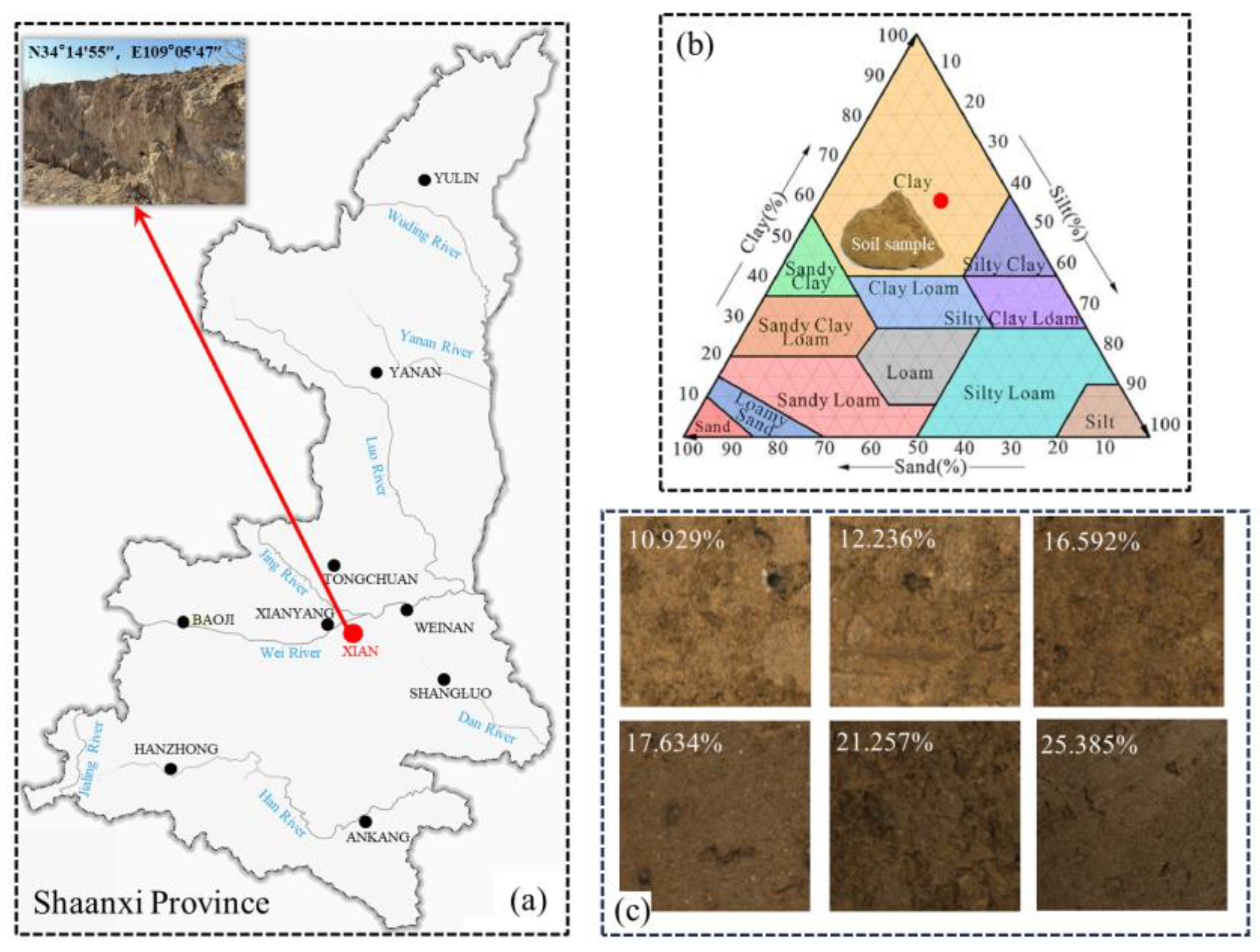
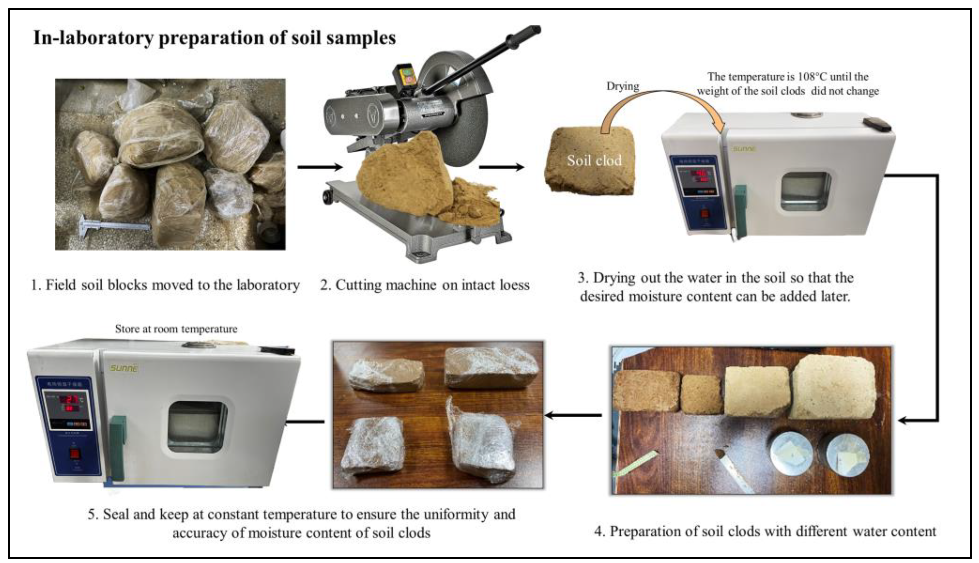
2.1. Soil Sampling and Preparation

The study area is located in the Bailu highland in Xi’an, Shaanxi Province, with sampling coordinates at 34°14′55″ N, 109°05′47″ E (Figure 2a). Shaanxi Province is one of the regions with the widest distribution of loess in China, and the Bailu highland is situated about 15 km southeast of Xi’an, Shaanxi Province. It is a representative loess mesa with an elevation ranging from 690 m to 780 m [37]. In our laboratory tests, we examined the properties of the soil, with the results shown in Table 1. According to the Soil Classification Guide [38] and FAO soil classification [39], the collected soil texture is classified as Clay, and the soil type is classified as Calcisols. The soil contains the organic carbon (OC) content of 9.3 g·kg−1, nitrogen (N) content of 1.7 g·kg−1, and a phosphorus content of 0.6 g·kg−1. This indicates a relatively high organic matter content in the soil.
In contrast to the use of remolded loess in other studies [13,33,40], we focused on studying undisturbed loess in its original state. To collect images of undisturbed loess, all soil samples were collected as intact blocks in field, which were then cut with a cutter to the desired dimensions in a laboratory. It is important to note that the minimum size for cutting is set at a width of 48 mm, height of 72 mm, and thickness of 20 mm. The determination of width and height ensures that the soil sample dimensions are larger than the imaging size of the camera, while the thickness consideration primarily focuses on the uniformity of moisture infiltration. As shown in Figure 3, the cut soil samples are then dried in an oven at 108 °C for more than 48 h, during which time they were weighed until there is no change in their weight; this is to ensure the accuracy of the different moisture contents configured in the experiment. These cut soil samples after drying are uniformly moistened with varying amounts of water. After moistening, the soil samples are sealed with plastic wrap and placed in a constant temperature chamber for 72 h to facilitate further even water penetration.

2.2. Automatic Soil Image Collection Platform

To capture images of undisturbed soil uniformly moistened with varying amounts of water, an automated image collection platform was designed, as depicted in Figure 4. The hardware consists of a camera and ring light, cutting tool, longitudinal feed unit, and transverse travel unit, while software has been developed based on MATLAB R2018b to facilitate the automated control of image acquisition and is installed on a computer. Industrial cameras are employed to capture soil images, equipped with a ring light as the sole lighting source. The cutting tool, as shown in Figure 4, is used to cut the soil after the images are collected. The longitudinal feed unit regulates the cutting feed rate, with each feed increment set at 1 mm. Considering the loss of moisture and to further ensure labeling accuracy, the longitudinal feed unit is fed a total of 5 mm for each moisture content category, i.e., the cutting tool makes five cuts, and we assume that the moisture content of the collected images is the same within these 5 mm. Once image capture is completed at a specific location, the transverse travel unit moves to the next position for image acquisition, ensuring non-overlapping image areas between consecutive captures. We collected the soil from each cut using an aluminum box and measured the moisture content by drying, and the SWC measurements were obtained. The experiments were conducted in a darkroom to eliminate external light interference during image acquisition, ensuring data accuracy and reliability.
A total of 530 original RGB images were captured across 19 categories (10.929%, 11.276%, 12.178%, 12.236%, 14.061%, 14.787%, 15.919%, 15.984%, 16.592%, 17.186%, 17.634%, 19.844%, 21.257%, 22.400%, 22.558%, 22.685%, 24.395%, 25.049%, and 25.385%), with a resolution of 3072 × 2048 pixels. After cropping, a total of 3175 cropped RGB images were collected, with a resolution of 256 × 256 pixels. The image format used was Bitmap (BMP), which is an uncompressed file. BMP avoids the loss of information and distortion that may be caused by other lossy compression formats. For dataset partitioning, 70% of the images were randomly selected for training the SWC recognition model, while the remaining 30% were used for testing the model. Within the training data, 20% was further randomly chosen as a validation dataset to assess the convergence of the model. To prevent overfitting [41] and enhance the robustness of the model, various data augmentation techniques were employed, including random crop, horizontal flip, vertical flip, 40% increase in brightness, and 40% decrease in brightness, as shown in Figure 5a–e. Additionally, data normalization was performed to improve the predictive accuracy and model fitting speed. Each feature variable was treated using normalization methods, which can boost the model’s performance. The normalization formula used for data normalization was as follows in Equation (1):
x o u t p u t c h a n n e l = x i n p u t c h a n n e l m e a n c h a n n e l s t d c h a n n e l
where channel is the three channels of the RGB color space, mean and std are the pixel mean and variance of the corresponding channel. By calculating, the mean of the three channels is (0.485, 0.456, 0.406) and the variance is (0.229, 0.224, 0.225).

2.3. PVP-Transformer-ED

The loess images primarily consist of soil regions and non-soil regions (porous areas, mineral composition zones), which are highly similar and recurrent. Inspired with previous studies that used only limited statistical variables to characterize the whole image [30,31,32,33], we propose an initial hypothesis that a small amount of pixel information can be utilized to substitute the entire image as the input for SWC recognition models. This hypothesis will significantly reduce the reliance on computational resources and lowers the barrier to application. Hence, a pre-trained encoder–decoder architecture (PVP-Transformer-ED) was designed to perform an image restoration task, as illustrated in Figure 6.
In PVP-Transformer-ED, the encoder is responsible for learning representations of visible patches, while the decoder takes the representations of visible and masked patches as the input to predict the RGB pixel values of the masked patch. By using sparse patches for soil image restoration, spatial redundancies and pre-training computational costs are reduced. Moreover, reconstructing the image based on this sparse relational information challenges the model to excel in pattern matching and correlation correction, preventing it from simply relying on lower-level statistical distributions in the image. PVP-Transformer-ED is required to truly understand an image by learning more abstract global information, which can then be fine-tuned from the encoder to the SWC recognition model. Further detailed explanations will be provided in the subsequent sections.

2.3.1. Masking Strategies

Various masking strategies have been proposed in the previous literature. For instance, [42] introduced a central region masking strategy, while BEiT [43] suggested a complex block masking strategy. More recent approaches such as MAE [44] and SiMmMIM [45] explored different patch sizes and mask ratios using a more direct random masking method that follows a uniform distribution to avoid potential center bias (i.e., having more masked patches near the center of the image). In the PVP-Transformer-ED, we employed a uniform random patch masking strategy for loess images. As depicted in Figure 6, a loess image of size (224 × 224 × 3) was initially divided into ( 224 P × 224 P ) equally sized patches with shapes of (P × P × 3). Subsequently, a portion of these patches was uniformly and randomly masked based on the mask ratio. In the experimental section, we compared the effects of different mask ratios and patch sizes. The high masking ratio random sampling (i.e., the proportion of patches removed) significantly reduced redundancy, creating a task that is not easily extrapolated from visible neighboring patches, as demonstrated in Figure 6. Finally, the highly sparse visible patches were fed into the encoder of the PVP-Transformer-ED for representation learning. Next, we will detail the encoder in the following section.

2.3.2. Encoder

The encoder in the PVP-Transformer-ED is responsible for modeling the potential feature representation of unmasked patches in soil images. Our encoder adopts a transformer architecture but is specifically applied to visible, unmasked patches. As illustrated in Figure 7d, the unmasked patches are flattened and mapped to one-dimensional vectors through Linear Embedding in the encoder. For example, each patch with a shape of (P × P × 3) is mapped to a tensor of length ( 3 · P 2 ) (referred to as tokens hereafter). Subsequently, Position Embedding is applied to add positional representations of the same shape as the tokens, serving as coordinates in the high-dimensional feature space of the image. The process is illustrated in Equation (2).
z 0 = x c l a , L E ( x p 1 ) , L E ( x p 2 ) , , L E ( x p n ) + E p o s ,   x c l a R 1 × P 2 · C ,   E p o s R N + 1 × P 2 · C , n [ 1 , N ]
In Equation (2), the input image x R H × W × C and the patch x p n R P × P × C , there are a total of N patches, with N = H · W P 2 . L E ( * ) denoting Linear Embedding, such that L E ( x p n ) R 1 × P 2 · C , where C represents the number of channels and P denotes the patch size. x c l a is a classification vector with the same shape as L E ( x p n ) , utilized for learning category information during the transformer architecture training process. To preserve spatial positional information among input image patches, it is also necessary to include positional encoding vectors for all image block vectors and classification vectors, as indicated by E p o s . Finally, output vector is z 0 .
The output tokens z 0   pass through a stack of L blocks consisting mainly of Layer Normalization (LN), Multi-Head Attention (MSA), and Multi-Layer Perceptron (MLP). The process is illustrated in Equations (3) and (4) by describing a single block as an example.
z l = M S A L N z l 1 + z l 1 , l = 1 L
z l = M L P L N z l + z l , l = 1 L
In Equation (3), the output vector z l 1 from the l 1 t h block undergoes layer normalization and is then subjected to attention computation, denoted as M S A L N z l 1 . Subsequently, this result is added as a residual connection to produce the intermediate vector z l for that block. Moving to Equation (4), the intermediate vector z l is passed through layer normalization and then processed by the MLP, represented as M L P L N z l . This is further augmented by a residual connection with z l to yield the final vector z l for that block. At this point, the computational process for the l th block concludes, and z l is subsequently input into the ( l + 1 )th block to repeat the computation processes described in Equations (3) and (4).

2.3.3. Decoder

The input to decoder of PVP-Transformer-ED comprises the complete set of patches, including encoded visible patches and masked patches. It is then used to predict the original signal in the masked regions of soil images. Each randomly initialized masked patch serves as a learnable vector to reveal the masked patches, and in the experimental section, we visualize this learning process. Position embedding is added to all tokens in this complete patch set; without them, the masked tokens lack information about their positions in the image. The core structure of the decoder is also based on the transformer architecture, but it operates independently from the transformer architecture in the encoder. Its input consists of the encoder’s input and positional information of the masked parts, while the output is the predicted values of the missing pixels. The final layer of the decoder is a linear projection, with the number of output channels is equal to the number of pixel values in the patches. The output of the encoder is reshaped to form the reconstructed image. In Equation (5), our loss function calculates the Mean Square Error (MSE) between the predicted image in pixel space and the original image, with the loss computed only on the masked patches.
M S E = p i p ^ i 2 N
where p i represents the original pixel value of the masked pixel, and p ^ i denotes the predicted pixel value by the architecture for the masked pixel. N denotes the total number of pixel values (in this case, N = 224 × 224). * represents the summation symbol, ranging from i = 1 to N.

2.4. Local Global SWC Recognition Regression Model (LG-SWC-R3 Model)

The encoder part of the PVP-Transformer-ED, which is capable of extracting “complete” features after the aforementioned pre-training, is extracted and fine-tuned on the Local Global SWC recognition regression model (LG-SWC-R3 model). The specific process is illustrated in Figure 8a above. This section focuses on introducing the LG-SWC-R3 model.
We adopt a hierarchical design with four stages to formulate the LG-SWC-R3 model, where the input resolution of each stage corresponds to 1 4 , 1 8 , 1 16 , 1 32 of the input model features. As illustrated in Equation (6), the features input x B , E , h , w to the model initially starting with a small kernel convolution stem layer [46] to embed the input feature:
x B , C ( j j = 1 ) ,   h 4 ,   w 4 = s t e m x B , E , h , w
where B represents the batch size, C denotes the channel dimension, h and w represent the height and width of the input feature. j belongs to the set {1, 2, 3, 4}.
Integrating local information can enhance the performance of the model [47]. PoolFormer [48] and EfficientFormer [49] utilize 3 × 3 average pooling layers as local token mixers. Substituting these layers with depth-wise convolutions (DWCONV) of the same kernel size may introduce additional parameters, but these negligible parameters not only do not incur latency overhead but also boost performance [46]. Furthermore, recent studies [47,50] suggest that injecting local information modeling layers into the Feed Forward Network layer [51] with minor overhead can also be beneficial for performance improvement. It is worth noting that by placing an extra 3 × 3 kernel size DWCONV in the FFN to capture local information, the function of the original local mixer (pooling or convolution) is replicated. Based on these observations, in the first stage, we designed a local FFN block, and the output of the local FFN block is further connected via residual connections, as depicted by Equation (7):
x B , C ( j j = 2 ) ,   h 8 ,   w 8 = S i , j · L o c a l   F F N x B , C ( j j = 1 ) ,   h 4 ,   w 4 + x B , C ( j j = 1 ) ,   h 4 ,   w 4
where S i , j represents a learnable layer scale [48]. x B , C ( j j = 1 ) ,   h 4 ,   w 4 is the output of Equation (6). L o c a l   F F N ( * ) is the Local FFN block, as shown in Figure 8c. We first use 1 × 1 convolutions for dimensionality reduction and add a segmented 3 × 3 kernel size DWCONV (DW.CONV3 × 3-BN) to the Local FFN block to extract local information, followed by 1 × 1 convolutions for dimensionality expansion, creating a localized FFN layer enabled with locality, where BN indicates the subsequent batch normalization. The computational flow of the Local FFN block is illustrated in Equation (8).
L o c a l   F F N x = C O N V 1 × 1 B N G E L U D W . C O N V 3 × 3 B N G E L U C O N V 1 × 1 B N x + x
The first two stages focus on capturing local information at high resolutions; therefore, we exclusively utilize the local FFN block with the inclusion of residual connections (Equations (7) and (8)). In the penultimate stage (Figure 8e), both the Local FFN block and the global MHSA block with the Global–Local Attention Downsampling Strategy are employed, with the inclusion of residual connections. The calculation flow of the penultimate stage is presented in Equation (9):
x B , C ( j j = 3 ) ,   h 16 ,   w 16 = L o c a l   F F N S i , j ·   G l o b a l M H S A A t t e n t i o n   D o w n s a m p l i n g [ P r o j x B , C ( j j = 2 ) ,   h 8 ,   w 8 ] + x B , C ( j j = 2 ) ,   h 8 ,   w 8
In the final stage, the Local–Global block is utilized, comprising the locally connected FFN block and the globally connected MHSA block (Figure 8d) with residual connections. The calculation flow of the final stage is presented in Equation (10):
x B , C ( j j = 4 ) ,   h 32 ,   w 32 = L o c a l   F F N S i , j · G l o b a l M H S A [ P r o j x B , C ( j j = 3 ) ,   h 16 ,   w 16 ] + x B , C ( j j = 3 ) ,   h 16 ,   w 16
The final output features are fed into a one-dimensional classifier layer to output the SWC. The predicted values are compared with the ground truth labels using a regression loss function commonly employed in regression models to assess their impact on recognition performance. In the experimental section, we separately demonstrate their effects on recognition performance.
In Section 2.4.1 and Section 2.4.2 below, we will introduce the global MHSA block and the Global MHSA block with the Attention Downsampling Strategy.

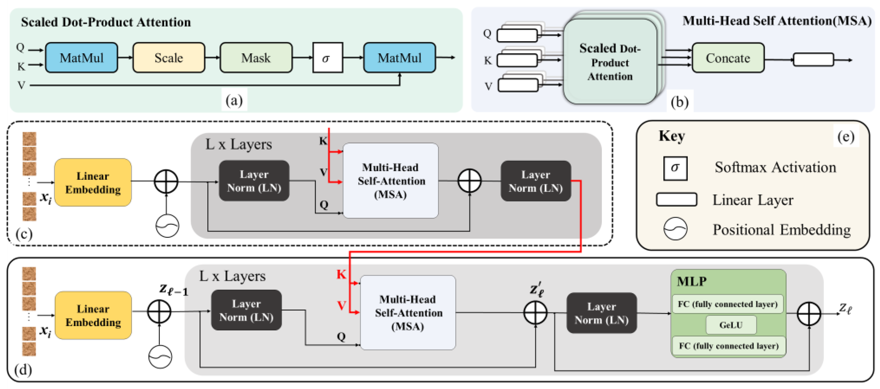
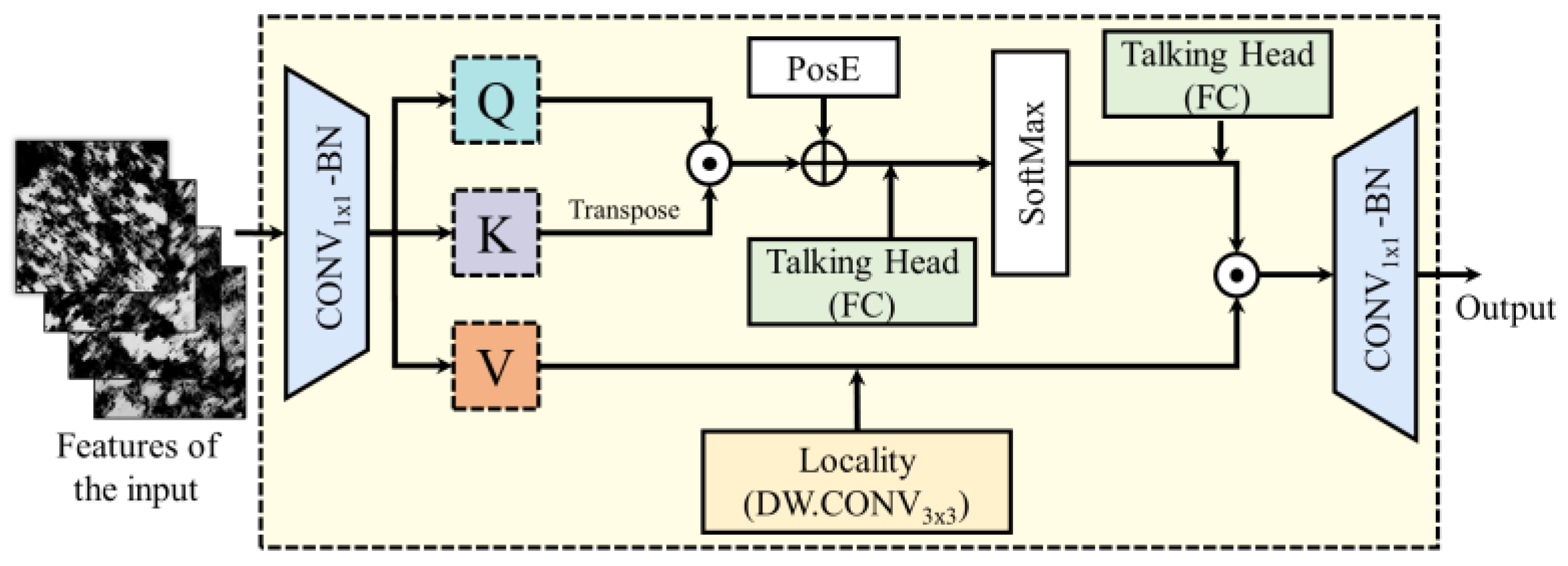
2.4.1. Global MHSA Block

The attention mechanism, such as Multi-Head Self-Attention (MHSA) [52], is beneficial for enhancing the model’s performance. As depicted in Figure 9, for the current input features, they are transformed into three distinct implicit spaces (Q, K, V) representing three different views of the same feature, where Queries (Q), Keys (K), and Values (V) are obtained by projecting input features using linear transformations. We first inject local information into the value matrix (V) by adding a DW.CONV with a kernel size of 3 × 3. Subsequently, we facilitate communication between attention heads by incorporating the fully connected layer over the head dimensions [53]. The process of the Global MHSA block is as Equation (11).
G l o b a l M H S A Q , K , V = T a l k i n g   H e a d [ s o f t m a x T a l k i n g   H e a d [ Q · K T + P o s E ] ] · D W . C O N V 3 × 3 V
where P o s E serves as a trainable attention bias for position encoding. T a l k i n g   H e a d [ * ] denotes a fully connected layer applied over the head dimensions. This process effectively integrates local information and facilitates information exchange between different heads during the attention calculation process.
However, applying it to high-resolution features in the early stages can lead to efficiency issues, as it incurs a quadratic time complexity relative to spatial resolution [54]. Therefore, we only employ the Global MHSA block in the final 1/32 spatial resolution, corresponding to the last stage, while designing the Global MHSA block with a global–local attention downsampling strategy.

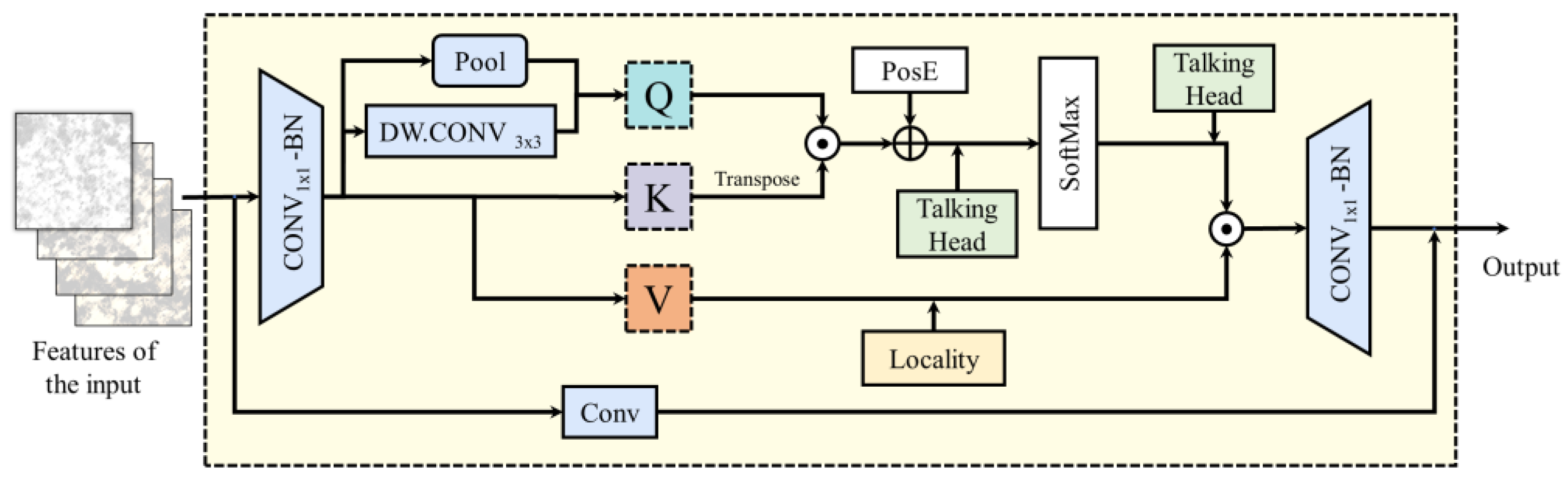
2.4.2. Global MHSA Block with Global–Local Attention Downsampling Strategy

We explored the effective application of the Global MHSA block to higher resolutions (early stages). Most vision models utilize strided convolutions or pooling layers for static and local downsampling, forming a hierarchical structure. Recent studies have started to investigate attention downsampling. For example, LeViT [55] and UniNet [56] propose reducing the feature resolution by half using attention mechanisms to achieve context-aware downsampling of the global receptive field. Specifically, the number of tokens in Q is halved, resulting in downsampling of the output of the attention module. In contrast, we devised a combination strategy as shown in Figure 10. To obtain downsampling Q, we employ the pooling layer for static local downsampling, 3 × 3 DWCONV for learnable local downsampling, and then merge and project the results into the Q dimension. Furthermore, the attention downsampling module is connected through residual connections [57] to regular CONV, forming locality and global dependency.

2.5. Model Performance Evaluation Metrics

Evaluation metrics are used to measure the difference between actual values and predicted values to assess the performance of regression models. Currently, there are numerous evaluation metrics used in SWC research. Among them, the Coefficient of Determination (R2) is commonly employed [58,59,60]. Authors in [29,58,61] utilized Root Mean Square Error (RMSE) for evaluation. Similarly, Mean Absolute Percentage Error (MAPE) [62] has been used for soil moisture estimation. In this study, we use R2, RMSE, MAPE, Mean Absolute Error [63] to evaluate the performance of the SWC recognition model. Based on these metrics, the most suitable model can be compared from multiple perspectives. Generally, models with high prediction accuracy and reliability exhibit the following traits: R2 trending towards 1, RMSE trending towards 0, MAPE trending towards 0, and MAE trending towards 0.

2.6. Implementation Settings

The experimental computer system used was Windows 10, with an Intel Core i5-12600KF CPU and a NVIDIA 2080ti GPU. The model’s code was executed on this computer system. The development language employed was Python 3.8, and the PyCharm 2022 platform was utilized for training and testing deep learning networks. All models were implemented using PyTorch 2.0.0 [64]. The optimization was performed using the AdamW optimizer [65] with a learning rate of 2 × 10 3 and a weight decay of 5 × 10 4 .

3. Experimental Results and Discussion

3.1. Performance Comparison of Different Models

We evaluated the performance of a range of SWC recognition models on the test set, including traditional machine learning regression models (Decision Tree [31], Random Forest [66], Support Vector Regression [63], Linear Regression [40], and Multilayer Perceptron [29]) and the LG-SWC-R3 model. The same as previous studies [30,31,32,33], the input independent variables for traditional machine learning models were the mean and variance of the RGB channels of soil images. During the evaluation process, we did not pre-train the PVP-Transformer-ED.
As shown in Table 2, in terms of R2, the LG-SWC-R3 model performed the best, reaching 0.950, followed by the Multilayer Perceptron and Linear Regression, which achieved 0.770 and 0.769, respectively. This indicates that the LG-SWC-R3 model better captures the moisture content variations. In terms of RMSE and MAE, the performance of the LG-SWC-R3 model is also the best, showing the lowest error levels of 1.351% and 0.886%, respectively. This means that the model’s recognitions are closer to the true values, demonstrating higher precision and accuracy. The Decision Tree performed the worst, with higher RMSE and MAE of 4.201% and 3.020%, respectively, indicating larger prediction deviations. The Support Vector Regression and Linear Regression performed relatively well, but still lag behind the LG-SWC-R3 model. The performances of the Random Forest and Multilayer Perceptron are moderate, slightly better than the Decision Tree, but still inferior to the Support Vector Regression and Linear Regression.
In conclusion, we found that different choices of traditional model had a significant effect on the recognition performance of SWC, which is similar to the results of previous research [32,67], but overall, they were significant and challenging to meet application requirements. In contrast, the LG-SWC-R3 model exhibited the best stability and satisfactory accuracy (R2 = 0.950, RMSE = 1.351%, MAPE = 0.081, MAE = 1.369%, which is lower than the maximum parallel error limit of 2% specified in [68]). To further analyze the recognition performance of the different models, we visualize their recognition scatterplots in Section 3.2.

3.2. Performance Analysis of Different Models

In this section, we visualize the recognition results of different models, as shown in Figure 11. Different subplots represent different models, where the straight red line within each subplot denotes the 1:1 line, with the scatter points representing the model’s recognition results, and the dashed line indicating the trend line of the results used to analyze the overall trend. From the perspective of trend lines, we observe that all models can capture the impact of SWC changes on soil images. However, the trend lines of Decision Tree [31] and Random Forest [66] deviate significantly from the 1:1 line, and Decision Tree’s identification results are mostly concentrated around similar values, consistent with their R2 results in Table 2, which are only 0.352 and 0.559, respectively. This accounts for the poor performance of these two models. While Support Vector Regression [63], Linear Regression [40], and Multilayer Perceptron [29] show some improvement in results, they fail to effectively identify images with SWC exceeding 20%, exhibiting a trend of underestimation compared to measured SWC. This inability contributes to the poor performance of Support Vector Regression, Linear Regression, and Multilayer Perceptron, reflecting a similar pattern in the Decision Tree and Random Forest. This may be because the response of soil image information to changes in SWC is not a straightforward relationship [13,31]. However, the results of the LG-SWC-R3 model effectively overcome the drawback of low sensitivity to high SWC and also respond well to soil images with lower SWC.

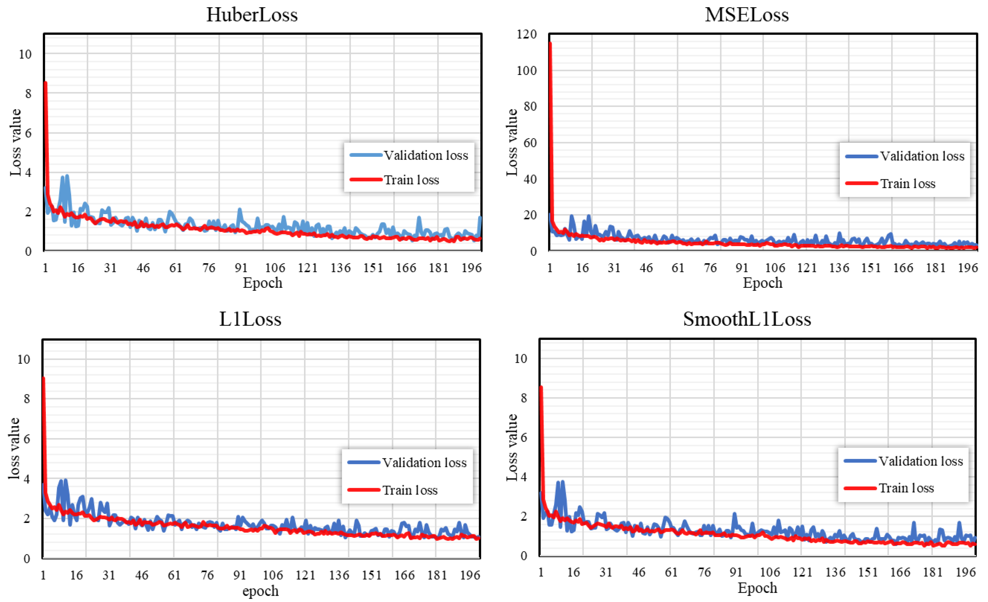
3.3. Comparison of Different Loss Functions

We conducted a comprehensive experiment aiming to compare the impact of different loss functions on the performance and convergence of the LG-SWC-R3 model. We selected MSE loss, L1 loss, SmoothL1 loss, and Huber loss as the four common regression model loss functions. We applied these loss functions individually to train the LG-SWC-R3 model and monitored the loss values on the training set as well as the performance on the validation set.
Surprisingly, as shown in Table 3, the choice of SmoothL1 loss and Huber loss seems to have little impact on the model’s performance, both in terms of prediction accuracy and outlier handling capabilities, while L1 Loss exhibits the best performance. This may be attributed to the fact that MSE loss penalizes large errors more significantly due to squaring [69]. L1 loss is less sensitive to outliers compared to MSE loss. SmoothL1 loss and Huber loss [70] both combine elements of both MSE and L1 loss, behaving like L1 loss for small errors and like MSE loss for large errors. In the context of soil images, aberrant image information can influence model training, and L1 loss is better equipped to handle such scenarios. Therefore, for the subsequent experiments, we selected it as the loss function for the LG-SWC-R3 model. Furthermore, as illustrated in Figure 12, we also observed that models trained with these loss functions demonstrated similar convergence performance on the validation set, without signs of overfitting [41]. This indicates that the LG-SWC-R3 model is able to learn critical patterns in the data within an appropriate timeframe without excessively fitting the training samples.

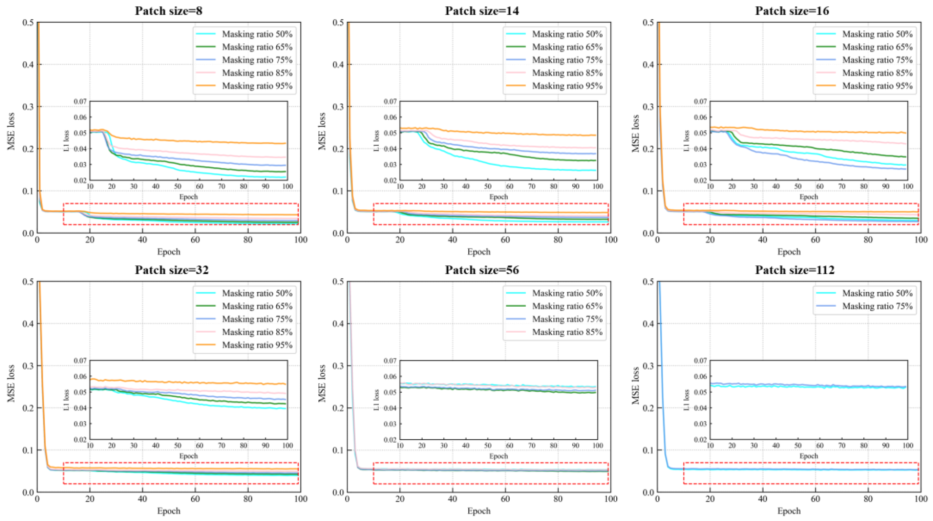
3.4. Stability Analysis of PVP-Transformer-ED

We conducted a thorough analysis on the impact of different hyperparameters (patch size and mask ratio) on the convergence behavior of the PVP-Transformer-ED. As illustrated in Figure 13, we observed that adjusting these hyperparameters did not significantly affect the convergence iterations of the PVP-Transformer-ED on the validation set, as it converged within 100 epochs regardless of the parameter settings. This suggests that the PVP-Transformer-ED can converge rapidly and effectively under various parameter configurations, exhibiting commendable optimization performance and stability. However, echoing the argument put forth in [44,45] regarding the significant challenge posed by larger patch sizes and mask ratios on reduction capabilities, upon a more detailed analysis of convergence behavior, we noticed that with the same mask ratio, as the patch size increased, the similarity between the reconstructed image and the original diminished, resulting in the loss stabilizing at a higher level. Likewise, maintaining a constant patch size while increasing the mask ratio also led to a decrease in the similarity between the predicted image and the original.

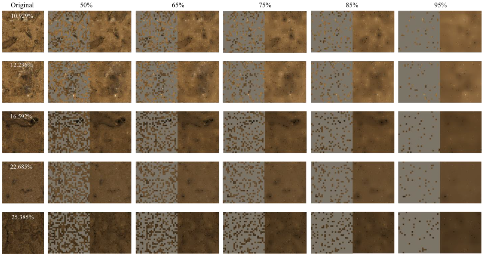
3.5. Masking Strategy

We selected a series of hyperparameters to investigate the effects of pre-training the PVP-Transformer-ED on the LG-SWC-R3 model. The baseline model refers to the LG-SWC-R3 model without pre-training using the PVP-Transformer-ED. The errors are recorded in Table 4.
Our exploration into the impact of different patch sizes on SWC recognition did not reveal significant differences in the original SWC recognition results. This suggests that the patch size may have a relatively minor impact on model performance in this task. Additionally, our experimental results revealed that as the mask ratio increased gradually, the identification errors also showed a corresponding rise, which aligns with the findings in [42,43,44,45]. However, even when masking 95% of the image, the maximum error was only R2 = 0.832, RMSE = 2.302%, MAPE = 0.092, and MAE = 1.546%. This demonstrates a high level of spatial redundancy in soil images. The approach of pre-training PVP-Transformer-ED and fine-tuning it on the SWC recognition model shows great potential in reducing the computational demands of the model.
Interestingly, the model exhibited insensitivity towards patch size. This could be ascribed to smaller patches offering restricted coverage of texture and other details in soil images, thereby enabling the model to perform recognitions relying on the remaining uncovered information. Conversely, larger patches might not provide as much reference information, yet they promote a certain level of generalization capability [44] in the encoder, leading to minimal impact on SWC recognition errors.

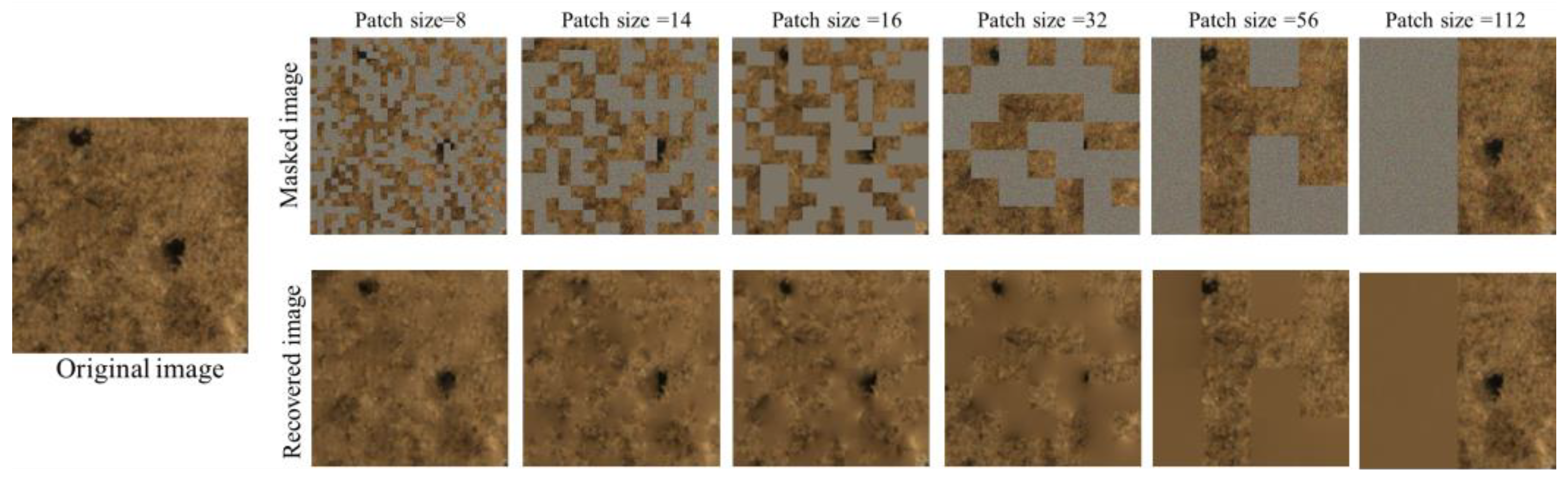
3.6. Visualization of PVP-Transformer-ED Restoration

We randomly selected five different soil images with varying moisture levels and visualized the restoration results of the PVP-Transformer-ED at different mask ratios, as shown in Figure 14. Regarding the mask ratio, we observed that different mask ratios can impact the quality of the restored images. A smaller mask ratio (e.g., 50%) is more effective in restoring detailed information in the missing areas while preserving more semantic features from the original image. This is attributed to the richer features and semantic information provided by the visible patches, enabling the predicted image to closely resemble the original image. As the mask ratio increases, the similarity between the predicted results and the original image decreases, as the model starts to interpret the semantic information of the image based on limited patches. This may result in less accurate details in the missing areas, a slight decrease in overall quality, and significant changes in the size and position of pore structures in the predicted image, indicating that the PVP-Transformer-ED is capable of generating images with new semantic information.
In Figure 15, images with various patch sizes are displayed to showcase the restoration effects under a fixed mask ratio of 0.5. It is evident that smaller patch sizes result in the better restoration of details, thereby indicating weaker generalization ability [44] in the learned representation. Restoration tasks on smaller-scale patch blocks may be more easily accomplished by neighboring pixels or textures. Larger patch sizes cover a significant portion of image details; for example, with patch sizes of 16 and 32, where the masked patches do not fully cover complex and intersecting non-soil regions (such as pores, cracks, and mineral composition information). In such cases, the PVP-Transformer-ED relies on limited non-soil regions for restoration, leading to creative predictive structures where non-soil regions are treated as generalizable information in terms of size and depth. However, as the patch size continues to increase, the predicted masked patches exhibit poorer detail representation, with texture information gradually replaced by overly smooth color blocks. This phenomenon becomes more pronounced with a patch size of 112.
Our study demonstrates a finding that is the same as the previous study that different hyperparameter settings do affect the experimental results to some extent [46,47,50,51]. In particular, through the adjustment of patch size and mask ratio, we have identified fluctuations in image clarity, detail retention, and overall visual impact. Our extensive analysis of experimental data has reaffirmed that modifying patch size and mask ratio can significantly impact the quality of generated images. These findings underscore the importance of judiciously selecting appropriate hyperparameters in practical applications to achieve a balance between hyperparameters, recognition accuracy, and computational efficiency.

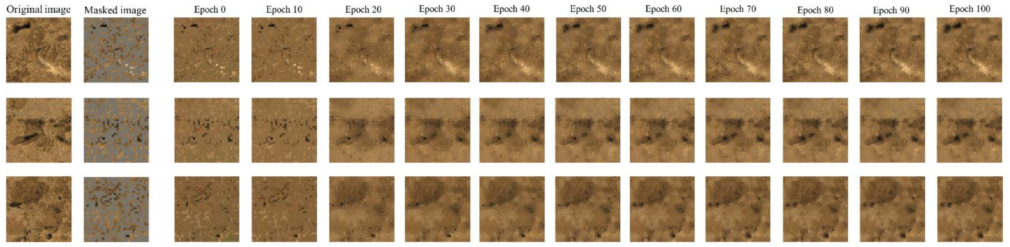
3.7. Visualization and Analysis of the Iterative Process of PVP-Transformer-ED

In this experiment (Figure 16), we take the example of a patch size of 8 and a ratio of 65%. We visualize the restoration effects of the PVP-Transformer-ED during the training process and document the corresponding results. We observe that the architecture’s reconstruction effect becomes progressively clearer with the increasing epochs. Edges and details gradually recover, and the image quality significantly improves. This result indicates that the PVP-Transformer-ED is learning better reconstruction representations. Additionally, the PVP-Transformer-ED successfully predicts key details in the original image (such as pores, cracks, mineral compositions, and other structures), avoiding excessive smoothing in patch prediction. This suggests that representations learned from visible patches can better capture the characteristics of the original image and preserve important detailed information during the prediction process.
Consistent with the experimental findings outlined in Section 3.4, we observe that the predictions made before 10 epochs tend to be more abstract. This vividly illustrates the progression of deep learning models, starting from learning simple features and gradually advancing towards more abstract and complex features, as elucidated in prior research [43]. As the iterations progress, pores, cracks, and mineral information are gradually restored, entering a stable phase after the 70th epoch. Surprisingly, in scenarios where specific masked patches fail to completely obscure intricate and overlapping non-soil regions (e.g., pores, cracks, and mineral constituents), the PVP-Transformer-ED reconstructs the image relying on the partially revealed non-soil areas, resulting in innovative predictive structures, such as a complete crack pattern being ultimately reconstructed as two cavities. This underscores the model’s robust learning capability, as evidenced in prior studies [52,57].

4. Conclusions

This study focuses on the undisturbed loess in the Bailu highland and addresses the issue of inadequate model accuracy and stability in previous research on SWC recognition based on images by developing a new deep learning model (LG-SWC-R3 model) to capture complex patterns and features in soil images. To overcome the computational cost and time required for handling large amounts of data, we conducted research from the perspective of reducing spatial redundancy in soil images. Specifically, we designed the PVP-Transformer-ED based on randomly masking soil images and predicting the original images using limited visible patches for this task. Subsequently, the pre-trained PVP-Transformer-ED was fine-tuned on the LG-SWC-R3 model. During the fine-tuning process, only sparse patches are required for SWC recognition, significantly reducing spatial redundancy and pre-training computational costs. The main conclusions are as follows.
1.
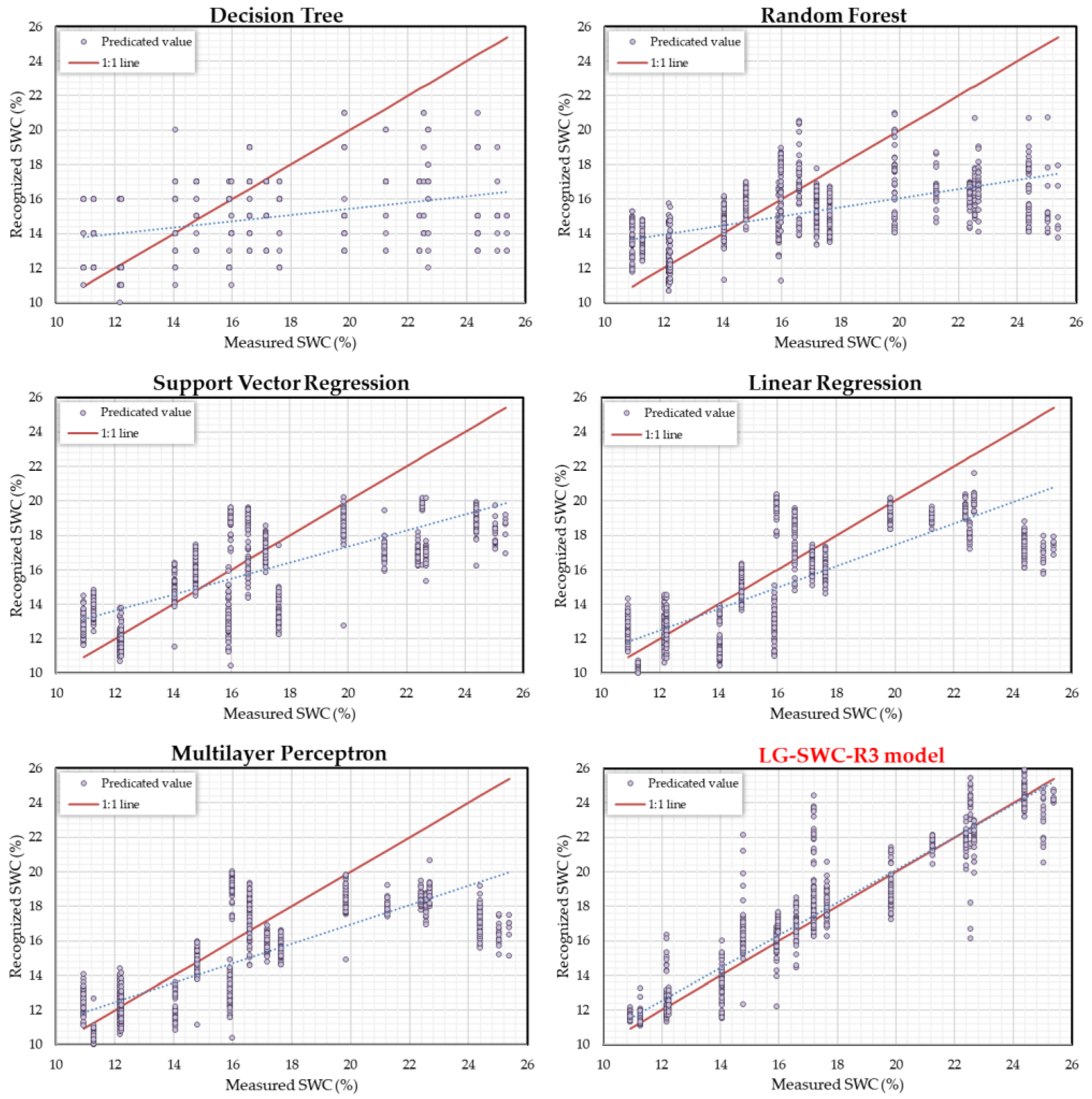
Evaluation of various SWC models revealed significant constraints with traditional machine learning models and highlighted the superior stability and satisfactory accuracy of the LG-SWC-R3 model. Visualizing the scatter plots in Section 3.2 further elucidated the performance differences among the models. While all models effectively captured moisture content changes in soil images, Decision Tree and Random Forest exhibited notable deviations from actual values. Additionally, Support Vector Regression, Linear Regression, and Multilayer Perceptron displayed a tendency to underestimate images with the SWC exceeding 20%. In contrast, the LG-SWC-R3 model demonstrated robustness in identifying images with both high and low SWC levels.
2.
Our pre-trained PVP-Transformer-ED can effectively restore the original soil image by predicting it from a limited number of unmasked patches. The core principle of PVP-Transformer-ED is its adeptness in computing and rectifying the relational attributes among input patches. In this regard, it operates by encoding a subset of randomly chosen patches to distill features and comprehend the image. This approach is suited for soil images, which typically possess heightened information redundancy owing to the pronounced local interconnections among pixels.
3.
Restoring visible sparse patches as the input serves a dual purpose: it not only diminishes spatial redundancy and alleviates the pre-training computational burden but also compels the architecture to transcend mere dependence on low-level statistical image distributions. This, in turn, necessitates a deeper and genuine comprehension of the image content. Remarkably, variations in hyperparameters like patch size and masked ratio imbue the model with a more “imaginative” capacity, facilitating the recognition of nuanced changes in pore and crack size and location within soil images. This enhanced perceptiveness aids the encoder in acquiring more versatile and generalizable representations.
4.
Fine-tuning the model after pre-training the PVP-Transformer-ED may slightly impact SWC recognition compared to recognizing the entire image. However, this impact remains within an acceptable range and offers substantial time and computational savings exceeding 50%. Such efficiency gains are particularly beneficial for applications in environments with limited computational resources and holds significant value for further deployment and utilization.
In our study, we have identified some limitations that need to be considered and addressed. Firstly, although the PVP-Transformer-ED demonstrates excellent performance in SWC identification, it still relies on a small fraction of pixels in the input images (i.e., affected by the masked ratio and patch size), which may limit the model’s generalization ability and applicability. Furthermore, while our method significantly reduces training time, and research results indicate that model errors remain within a reasonable range, the robustness and stability of the model across different soil types need further validation due to variations in mineral composition and organic matter among different soil types. Therefore, we recognize that improving the model’s generalization ability, reducing the reliance on input pixels, and further optimizing model performance are important directions for future research. By continuously refining and adjusting our approach, we can better address these limitations, enhance the accuracy and efficiency of the model, and better meet the practical application requirements.

Author Contributions

Conceptualization, Z.D.; data curation, Y.Z. and H.Z.; formal analysis, H.L. (Hengxing Lan) and Z.D.; funding acquisition, H.L. (Hengxing Lan); investigation, E.W.; methodology, Y.Z., H.Z. and Z.D.; project administration, H.L. (Hengxing Lan) and Z.D.; software, Y.L. and E.W.; supervision, E.W.; validation, D.S.; visualization, Y.Z. and D.S.; writing—original draft, Y.Z.; writing—review and editing, Y.Z., H.Z., Y.L., H.L. (Honggang Liu) and D.S. All authors have read and agreed to the published version of the manuscript.

Funding

This research was funded by National Natural Science Foundation of China, grant number 41927806.

Data Availability Statement

The data presented in this study are available on request from the corresponding author. The data are not publicly available due to confidentiality of datasets.

Conflicts of Interest

Author Yunchuang Li, Honggang Liu were employed by the company China Construction First Group Corporation Limited. The remaining authors declare that the research was conducted in the absence of any commercial or financial relationships that could be construed as a potential conflict of interest.

References

  1. White, R.E. Principles and Practice of Soil Science: The Soil as a Natural Resource; John Wiley & Sons: Hoboken, NJ, USA, 2005. [Google Scholar]
  2. Hossain, M.; Lamb, D.; Lockwood, P.; Frazier, P. EM38 for volumetric soil water content estimation in the root-zone of deep vertosol soils. Comput. Electron. Agric. 2010, 74, 100–109. [Google Scholar] [CrossRef]
  3. Dobriyal, P.; Qureshi, A.; Badola, R.; Hussain, S.A. A review of the methods available for estimating soil moisture and its implications for water resource management. J. Hydrol. 2012, 458, 110–117. [Google Scholar] [CrossRef]
  4. Chen, S.; Lou, F.; Tuo, Y.; Tan, S.; Peng, K.; Zhang, S.; Wang, Q. Prediction of Soil Water Content Based on Hyperspectral Reflectance Combined with Competitive Adaptive Reweighted Sampling and Random Frog Feature Extraction and the Back-Propagation Artificial Neural Network Method. Water 2023, 15, 2726. [Google Scholar] [CrossRef]
  5. Chakraborty, D.; Nagarajan, S.; Aggarwal, P.; Gupta, V.; Tomar, R.; Garg, R.; Sahoo, R.; Sarkar, A.; Chopra, U.K.; Sarma, K.S. Effect of mulching on soil and plant water status, and the growth and yield of wheat (Triticum aestivum L.) in a semi-arid environment. Agric. Water Manag. 2008, 95, 1323–1334. [Google Scholar] [CrossRef]
  6. Coppola, A.; Dragonetti, G.; Sengouga, A.; Lamaddalena, N.; Comegna, A.; Basile, A.; Noviello, N.; Nardella, L. Identifying optimal irrigation water needs at district scale by using a physically based agro-hydrological model. Water 2019, 11, 841. [Google Scholar] [CrossRef]
  7. Rahardjo, H.; Kim, Y.; Satyanaga, A. Role of unsaturated soil mechanics in geotechnical engineering. Int. J. Geo-Eng. 2019, 10, 8. [Google Scholar] [CrossRef]
  8. Gens, A. Soil–environment interactions in geotechnical engineering. Géotechnique 2010, 60, 3–74. [Google Scholar] [CrossRef]
  9. Al-Rawas, A.A. State-of-the-art-review of collapsible soils. Sultan Qaboos Univ. J. Sci. [SQUJS] 2000, 5, 115–135. [Google Scholar] [CrossRef]
  10. Negro, A., Jr.; Karlsrud, K.; Srithar, S.; Ervin, M.; Vorster, E. Prediction, monitoring and evaluation of performance of geotechnical structures. In Proceedings of the 17th International Conference on Soil Mechanics and Geotechnical Engineering (Volumes 1, 2, 3 and 4), Alexandria, Egypt, 5–9 October 2009; pp. 2930–3005. [Google Scholar]
  11. Marino, P.; Peres, D.J.; Cancelliere, A.; Greco, R.; Bogaard, T.A. Soil moisture information can improve shallow landslide forecasting using the hydrometeorological threshold approach. Landslides 2020, 17, 2041–2054. [Google Scholar] [CrossRef]
  12. Furtak, K.; Wolińska, A. The impact of extreme weather events as a consequence of climate change on the soil moisture and on the quality of the soil environment and agriculture—A review. Catena 2023, 231, 107378. [Google Scholar] [CrossRef]
  13. Liu, G.; Tian, S.; Xu, G.; Zhang, C.; Cai, M. Combination of effective color information and machine learning for rapid prediction of soil water content. J. Rock Mech. Geotech. Eng. 2023, 15, 2441–2457. [Google Scholar] [CrossRef]
  14. Walker, J.P.; Willgoose, G.R.; Kalma, J.D. In situ measurement of soil moisture: A comparison of techniques. J. Hydrol. 2004, 293, 85–99. [Google Scholar] [CrossRef]
  15. Yin, Z.; Lei, T.; Yan, Q.; Chen, Z.; Dong, Y. A near-infrared reflectance sensor for soil surface moisture measurement. Comput. Electron. Agric. 2013, 99, 101–107. [Google Scholar] [CrossRef]
  16. Su, S.L.; Singh, D.N.; Baghini, M.S. A critical review of soil moisture measurement. Measurement 2014, 54, 92–105. [Google Scholar] [CrossRef]
  17. Lakshmi, V. Remote sensing of soil moisture. Int. Sch. Res. Not. 2013, 2013, 424178. [Google Scholar] [CrossRef]
  18. Peng, J.; Shen, Z.; Zhang, W.; Song, W. Deep-Learning-Enhanced CT Image Analysis for Predicting Hydraulic Conductivity of Coarse-Grained Soils. Water 2023, 15, 2623. [Google Scholar] [CrossRef]
  19. Snapir, B.; Hobbs, S.; Waine, T. Roughness measurements over an agricultural soil surface with Structure from Motion. ISPRS J. Photogramm. Remote Sens. 2014, 96, 210–223. [Google Scholar] [CrossRef]
  20. Wang, D.; Si, Y.; Shu, Z.; Wu, A.; Wu, Y.; Li, Y. An image-based soil type classification method considering the impact of image acquisition distance factor. J. Soils Sediments 2023, 23, 2216–2233. [Google Scholar] [CrossRef]
  21. Swetha, R.; Bende, P.; Singh, K.; Gorthi, S.; Biswas, A.; Li, B.; Weindorf, D.C.; Chakraborty, S. Predicting soil texture from smartphone-captured digital images and an application. Geoderma 2020, 376, 114562. [Google Scholar] [CrossRef]
  22. Pires, L.F.; Cássaro, F.A.M.; Bacchi, O.O.S.; Reichardt, K. Non-destructive image analysis of soil surface porosity and bulk density dynamics. Radiat. Phys. Chem. 2011, 80, 561–566. [Google Scholar] [CrossRef]
  23. Shi, T.; Cui, L.; Wang, J.; Fei, T.; Chen, Y.; Wu, G. Comparison of multivariate methods for estimating soil total nitrogen with visible/near-infrared spectroscopy. Plant Soil 2013, 366, 363–375. [Google Scholar] [CrossRef]
  24. Meng, C.; Yang, W.; Bai, Y.; Li, H.; Zhang, H.; Li, M. Research of soil surface image occlusion removal and inpainting based on GAN used for estimation of farmland soil moisture content. Comput. Electron. Agric. 2023, 212, 108155. [Google Scholar] [CrossRef]
  25. Gadi, V.K.; Garg, A.; Manogaran, I.P.; Sekharan, S.; Zhu, H.-H. Understanding soil surface water content using light reflection theory: A novel color analysis technique considering variability in light intensity. J. Test. Eval. 2020, 48, 4053–4066. [Google Scholar] [CrossRef]
  26. Parera, F.; Pinyol, N.M.; Alonso, E.E. Massive, continuous, and non-invasive surface measurement of degree of saturation by shortwave infrared images. Can. Geotech. J. 2021, 58, 749–762. [Google Scholar] [CrossRef]
  27. Liu, W.; Baret, F.; Gu, X.; Tong, Q.; Zheng, L.; Zhang, B. Relating soil surface moisture to reflectance. Remote Sens. Environ. 2002, 81, 238–246. [Google Scholar] [CrossRef]
  28. Maltese, A.; Minacapilli, M.; Cammalleri, C.; Ciraolo, G.; D’Asaro, F. A thermal inertia model for soil water content retrieval using thermal and multispectral images. In Proceedings of the Remote Sensing for Agriculture, Ecosystems, and Hydrology XII, Toulouse, France, 22 October 2010; pp. 273–280. [Google Scholar]
  29. Zanetti, S.S.; Cecilio, R.A.; Alves, E.G.; Silva, V.H.; Sousa, E.F. Estimation of the moisture content of tropical soils using colour images and artificial neural networks. Catena 2015, 135, 100–106. [Google Scholar] [CrossRef]
  30. Persson, M. Estimating surface soil moisture from soil color using image analysis. Vadose Zone J. 2005, 4, 1119–1122. [Google Scholar] [CrossRef]
  31. Dos Santos, J.F.; Silva, H.R.; Pinto, F.A.; Assis, I.R.D. Use of digital images to estimate soil moisture. Rev. Bras. Eng. Agrícola Ambient. 2016, 20, 1051–1056. [Google Scholar] [CrossRef]
  32. Taneja, P.; Vasava, H.B.; Fathololoumi, S.; Daggupati, P.; Biswas, A. Predicting soil organic matter and soil moisture content from digital camera images: Comparison of regression and machine learning approaches. Can. J. Soil Sci. 2022, 102, 767–784. [Google Scholar] [CrossRef]
  33. Kim, D.; Kim, T.; Jeon, J.; Son, Y. Convolutional Neural Network-Based Soil Water Content and Density Prediction Model for Agricultural Land Using Soil Surface Images. Appl. Sci. 2023, 13, 2936. [Google Scholar] [CrossRef]
  34. Zhu, Y.; Wang, Y.; Shao, M. Using soil surface gray level to determine surface soil water content. Sci. China Earth Sci. 2010, 53, 1527–1532. [Google Scholar] [CrossRef]
  35. Hosseini, R.; Sinz, F.; Bethge, M. Lower bounds on the redundancy of natural images. Vis. Res. 2010, 50, 2213–2222. [Google Scholar] [CrossRef] [PubMed]
  36. Yang, C.; Bruzzone, L.; Zhao, H.; Tan, Y.; Guan, R. Superpixel-based unsupervised band selection for classification of hyperspectral images. IEEE Trans. Geosci. Remote Sens. 2018, 56, 7230–7245. [Google Scholar] [CrossRef]
  37. Peng, J.; Wang, Q.; Zhuang, J.; Leng, Y.; Fan, Z.; Wang, S. Triggered factors and motion simulation of “9-17” baqiao catastrophic landslide. J. Eng. Geol. 2015, 23, 747–754. [Google Scholar] [CrossRef]
  38. Moreno-Maroto, J.M.; Alonso-Azcarate, J. Evaluation of the USDA soil texture triangle through Atterberg limits and an alternative classification system. Appl. Clay Sci. 2022, 229, 106689. [Google Scholar] [CrossRef]
  39. Fao, W. World reference base for soil resources. International soil classification system for naming soils and creating legends for soil maps. World Soil Resour. Rep. 2014, 106, 12–21. [Google Scholar]
  40. Hajjar, C.S.; Hajjar, C.; Esta, M.; Chamoun, Y.G. Machine learning methods for soil moisture prediction in vineyards using digital images. In Proceedings of the E3S Web of Conferences, Tallinn, Estonia, 6–9 September 2020; p. 02004. [Google Scholar]
  41. Xu, J.J.; Zhang, H.; Tang, C.S.; Cheng, Q.; Tian, B.G.; Liu, B.; Shi, B. Automatic soil crack recognition under uneven illumination condition with the application of artificial intelligence. Eng. Geol. 2022, 296, 106495. [Google Scholar] [CrossRef]
  42. Pathak, D.; Krahenbuhl, P.; Donahue, J.; Darrell, T.; Efros, A.A. Context encoders: Feature learning by inpainting. In Proceedings of the IEEE Conference on Computer Vision and Pattern Recognition, Las Vegas, NV, USA, 27–30 June 2016; pp. 2536–2544. [Google Scholar]
  43. Bao, H.; Dong, L.; Piao, S.; Wei, F. Beit: Bert pre-training of image transformers. arXiv 2021, arXiv:2106.08254. [Google Scholar] [CrossRef]
  44. He, K.; Chen, X.; Xie, S.; Li, Y.; Dollár, P.; Girshick, R. Masked autoencoders are scalable vision learners. In Proceedings of the IEEE/CVF Conference on Computer Vision and Pattern Recognition, New Orleans, LA, USA, 18–24 June 2022; pp. 16000–16009. [Google Scholar]
  45. Xie, Z.; Zhang, Z.; Cao, Y.; Lin, Y.; Bao, J.; Yao, Z.; Dai, Q.; Hu, H. Simmim: A simple framework for masked image modeling. In Proceedings of the IEEE/CVF Conference on Computer Vision and Pattern Recognition, New Orleans, LA, USA, 18–24 June 2022; pp. 9653–9663. [Google Scholar]
  46. Li, Y.; Hu, J.; Wen, Y.; Evangelidis, G.; Salahi, K.; Wang, Y.; Tulyakov, S.; Ren, J. Rethinking vision transformers for mobilenet size and speed. In Proceedings of the IEEE/CVF International Conference on Computer Vision, Paris, France, 2–3 October 2023; pp. 16889–16900. [Google Scholar]
  47. Cai, H.; Gan, C.; Han, S. Efficientvit: Enhanced linear attention for high-resolution low-computation visual recognition. arXiv 2022, arXiv:2205.14756. [Google Scholar] [CrossRef]
  48. Yu, W.; Luo, M.; Zhou, P.; Si, C.; Zhou, Y.; Wang, X.; Feng, J.; Yan, S. Metaformer is actually what you need for vision. In Proceedings of the IEEE/CVF Conference on Computer Vision and Pattern Recognition, New Orleans, LA, USA, 18–24 June 2022; pp. 10819–10829. [Google Scholar]
  49. Li, Y.; Yuan, G.; Wen, Y.; Hu, J.; Evangelidis, G.; Tulyakov, S.; Wang, Y.; Ren, J. Efficientformer: Vision transformers at mobilenet speed. Adv. Neural Inf. Process. Syst. 2022, 35, 12934–12949. [Google Scholar] [CrossRef]
  50. Gong, C.; Wang, D.; Li, M.; Chen, X.; Yan, Z.; Tian, Y.; Chandra, V. Nasvit: Neural architecture search for efficient vision transformers with gradient conflict aware supernet training. In Proceedings of the International Conference on Learning Representations, Virtual Event, 25–29 April 2022. [Google Scholar]
  51. LeCun, Y.; Bottou, L.; Bengio, Y.; Haffner, P. Gradient-based learning applied to document recognition. Proc. IEEE 1998, 86, 2278–2324. [Google Scholar] [CrossRef]
  52. Voita, E.; Talbot, D.; Moiseev, F.; Sennrich, R.; Titov, I. Analyzing multi-head self-attention: Specialized heads do the heavy lifting, the rest can be pruned. arXiv 2019, arXiv:1905.09418. [Google Scholar] [CrossRef]
  53. Shazeer, N.; Lan, Z.; Cheng, Y.; Ding, N.; Hou, L. Talking-heads attention. arXiv 2020, arXiv:2003.02436. [Google Scholar] [CrossRef]
  54. Liu, Z.; Lin, Y.; Cao, Y.; Hu, H.; Wei, Y.; Zhang, Z.; Lin, S.; Guo, B. Swin transformer: Hierarchical vision transformer using shifted windows. In Proceedings of the IEEE/CVF International Conference on Computer Vision, Montreal, BC, Canada, 11–17 October 2021; pp. 10012–10022. [Google Scholar]
  55. Graham, B.; El-Nouby, A.; Touvron, H.; Stock, P.; Joulin, A.; Jégou, H.; Douze, M. Levit: A vision transformer in convnet’s clothing for faster inference. In Proceedings of the IEEE/CVF International Conference on Computer Vision, Paris, France, 2–3 October 2021; pp. 12259–12269. [Google Scholar]
  56. Liu, J.; Huang, X.; Song, G.; Li, H.; Liu, Y. Uninet: Unified architecture search with convolution, transformer, and mlp. In Proceedings of the European Conference on Computer Vision, Tel Aviv, Israel, 23–27 October 2022; pp. 33–49. [Google Scholar]
  57. He, K.; Zhang, X.; Ren, S.; Sun, J. Deep residual learning for image recognition. In Proceedings of the IEEE Conference on Computer Vision and Pattern Recognition, Las Vegas, NV, USA, 27–30 June 2016; pp. 770–778. [Google Scholar]
  58. Sakti, M.; Ariyanto, D. Estimating soil moisture content using red-green-blue imagery from digital camera. In Proceedings of the IOP Conference Series: Earth and Environmental Science, Langkawi, Malaysia, 4–5 December 2018; p. 012004. [Google Scholar]
  59. Taneja, P.; Vasava, H.K.; Daggupati, P.; Biswas, A. Multi-algorithm comparison to predict soil organic matter and soil moisture content from cell phone images. Geoderma 2021, 385, 114863. [Google Scholar] [CrossRef]
  60. Aitkenhead, M.J.; Poggio, L.; Wardell-Johnson, D.; Coull, M.C.; Rivington, M.; Black, H.; Yacob, G.; Boke, S.; Habte, M. Estimating soil properties from smartphone imagery in Ethiopia. Comput. Electron. Agric. 2020, 171, 105322. [Google Scholar] [CrossRef]
  61. Döpper, V.; Rocha, A.D.; Berger, K.; Gränzig, T.; Verrelst, J.; Kleinschmit, B.; Förster, M. Estimating soil moisture content under grassland with hyperspectral data using radiative transfer modelling and machine learning. Int. J. Appl. Earth Obs. Geoinf. 2022, 110, 102817. [Google Scholar] [CrossRef]
  62. Yu, J.; Tang, S.; Li, Z.; Zheng, W.; Wang, L.; Wong, A.; Xu, L. A deep learning approach for multi-depth soil water content prediction in summer maize growth period. IEEE Access 2020, 8, 199097–199110. [Google Scholar] [CrossRef]
  63. Hossain, M.R.H.; Kabir, M.A. Machine Learning Techniques for Estimating Soil Moisture from Smartphone Captured Images. Agriculture 2023, 13, 574. [Google Scholar] [CrossRef]
  64. Paszke, A.; Gross, S.; Massa, F.; Lerer, A.; Bradbury, J.; Chanan, G.; Killeen, T.; Lin, Z.; Gimelshein, N.; Antiga, L. Pytorch: An imperative style, high-performance deep learning library. Adv. Neural Inf. Process. Syst. 2019, 32, 8026–8037. [Google Scholar]
  65. Loshchilov, I.; Hutter, F. Decoupled weight decay regularization. arXiv 2017, arXiv:1711.05101. [Google Scholar] [CrossRef]
  66. Rodriguez-Galiano, V.; Sanchez-Castillo, M.; Chica-Olmo, M.; Chica-Rivas, M. Machine learning predictive models for mineral prospectivity: An evaluation of neural networks, random forest, regression trees and support vector machines. Ore Geol. Rev. 2015, 71, 804–818. [Google Scholar] [CrossRef]
  67. Fang, L.; Zhan, X.; Yin, J.; Liu, J.; Schull, M.; Walker, J.P.; Wen, J.; Cosh, M.H.; Lakhankar, T.; Collins, C.H. An intercomparison study of algorithms for downscaling SMAP radiometer soil moisture retrievals. J. Hydrometeorol. 2020, 21, 1761–1775. [Google Scholar] [CrossRef]
  68. GB/T 50123-2019; China national standards: Standard for geotechnical testing method. Standardization Administration of China, Ministry of Water Resources, China Planning Press: Beijing, China, 2019. (In Chinese)
  69. Han, X.; Papyan, V.; Donoho, D.L. Neural collapse under mse loss: Proximity to and dynamics on the central path. arXiv 2021, arXiv:2106.02073. [Google Scholar] [CrossRef]
  70. Wang, Q.; Ma, Y.; Zhao, K.; Tian, Y. A comprehensive survey of loss functions in machine learning. Ann. Data Sci. 2020, 9, 5500. [Google Scholar] [CrossRef]
Figure 1. The research framework of this study.
Water 16 01133 g001
Figure 2. (a) Sampling location of undisturbed soil samples, (b) soil texture triangle [38] and the type to which the sampled soil belongs, (c) partial display of collected soil images.
Water 16 01133 g002
Figure 3. Soil sample laboratory preparation for preparing samples with varying moisture levels for image collection.
Water 16 01133 g003
Figure 4. Undisturbed loess automatic image collection platform.
Water 16 01133 g004
Figure 5. Soil image data augmentation methods.
Water 16 01133 g005
Figure 6. Patch-based Visual Perception Encoder–Decoder Architecture-based transformer (PVP-Transformer-ED).
Water 16 01133 g006
Figure 7. Transformer architecture in encoder and decoder. (a) Scaled Dot–Product Attention in Multi-Head Self Attention (MSA), (b) MSA, (c,d) are the overall architecture in transformer architecture, (e) The key of this figure.
Water 16 01133 g007
Figure 8. (a) Process architecture involves pretraining on the PVP-Transformer-ED followed by fine-tuning on the SWC model, (b) designed Local Global SWC recognition regression model (LG-SWC-R3 model), (c) local FFN block in the LG-SWC-R3 model, (d) local–global block in the LG-SWC-R3 model, (e) local–global block with attention downsampling strategy in the LG-SWC-R3 model.
Water 16 01133 g008
Figure 9. Global MHSA block structure.
Water 16 01133 g009
Figure 10. Global MHSA block with Global–Local Attention Downsampling Strategy.
Water 16 01133 g010
Figure 11. SWC recognition results of the scatterplot of the six models. The dashed line is the linear trend line of the recognition results.
Water 16 01133 g011
Figure 12. Convergence of the LG-SWC-R3 model under different regression loss functions on the validation set.
Water 16 01133 g012
Figure 13. Convergence analysis of the PVP-Transformer-ED under different hyperparameters (patch size and mask ratio).
Water 16 01133 g013
Figure 14. Visualization of PVP-Transformer-ED restoration with a patch size of 16 for masking. The first column displays the original image, while every two columns afterwards represent a different combination, each indicating a distinct mask ratio.
Water 16 01133 g014
Figure 15. Visualizing the restoration results of the PVP-Transformer-ED with different patch sizes under a mask ratio of 0.5.
Water 16 01133 g015
Figure 16. Visualization of predicting masked patches based on visible patches in the training iterative process of PVP-Transformer-ED.
Water 16 01133 g016
Table 1. Soil properties at the sampling location.
Study SitesSoil TextureSoil TypeSand
(%)
Slit
(%)
Clay
(%)
Organic Carbon (OC)
(g·kg−1)
Nitrogen (N)
(g·kg−1)
Phosphorous (P)
(g·kg−1)
Bailu
highland
ClayCalcisols11.730.657.79.31.70.6
Table 2. Accuracy assessment of SWC recognition models under different evaluation metrics.
SWC Recognition ModelR2RMSE (%)MAPEMAE (%)
Decision Tree [31]0.3524.2010.2063.020
Random Forest [66]0.5593.6570.1562.745
Support Vector Regression [63]0.7172.9680.1412.379
Linear Regression [40]0.7692.8820.1272.169
Multilayer Perceptron [29]0.7703.0040.1262.243
LG-SWC-R3 model0.9501.3510.0540.886
Table 3. Comparison of the performance of different loss functions on evaluation metrics.
Loss FunctionR2RMSE (%)MAPEMAE (%)
HuberLoss0.9491.3820.0520.847
L1Loss0.9531.2610.0490.820
MSELoss0.9321.5630.0641.034
SmoothL1Loss0.9501.3510.0540.886
Table 4. An ablation study on the impact of different patch sizes and mask ratios on the LG-SWC-R3 model.
ModelMasked Patch SizeMasking RationR2RMSEMAPEMAE
Baseline××0.9501.3510.0540.886
80.50.9421.4090.0500.838
0.650.9171.5880.0671.042
0.750.9031.7840.0621.029
0.850.9221.7450.0711.123
0.950.8322.3020.0921.546
140.50.9271.5710.0580.961
0.650.9221.6050.0591.013
0.750.8961.8400.0661.138
0.850.9121.8410.0781.262
0.950.8622.1040.0861.413
160.50.9301.5400.0610.987
0.650.9291.5580.0590.983
PVP-Transformer-ED 0.750.9381.5430.0621.002
0.850.8961.8480.0631.109
0.950.8762.0450.0811.377
320.50.9251.5780.0560.944
0.650.9131.7250.0621.081
0.750.9001.8190.0641.115
0.850.8552.1850.0721.261
0.950.8392.2490.0931.535
560.50.9311.5770.0570.916
0.650.9091.7450.0621.026
0.750.8901.9360.0711.164
0.850.8821.9690.0761.294
1120.50.9311.5550.0610.982
0.750.8841.9340.0721.216
Disclaimer/Publisher’s Note: The statements, opinions and data contained in all publications are solely those of the individual author(s) and contributor(s) and not of MDPI and/or the editor(s). MDPI and/or the editor(s) disclaim responsibility for any injury to people or property resulting from any ideas, methods, instructions or products referred to in the content.

