Article

Future Trade-Off for Water Resource Allocation: The Role of Land Cover/Land Use Change

by
Onesmo Zakaria Sigalla
1,2,*,
Sekela Twisa
3,
Nyemo Amos Chilagane
4,
Mohamed Fadhili Mwabumba
5,
Juma Rajabu Selemani
1 and
Patrick Valimba
6
1
Nelson Mandela-African Institution of Science and Technology, Nelson Mandela Road, Arusha P.O. Box 447, Tanzania
2
Rain Drop Initiative, 109 Regent Estate, Mikocheni, Dar es Salaam P.O. Box 8703, Tanzania
3
Water Resource Center of Excellence, Water Resource Department, Ministry of Water, Dodoma P.O. Box 456, Tanzania
4
Tanzania Research and Conservation Organization, Morogoro P.O. Box 6873, Tanzania
5
Tanzania Meteorological Authority, Dar es Salaam P.O. Box 3056, Tanzania
6
Department of Water Resources Engineering, College of Engineering and Technology, University of Dar es Salaam, Dar es Salaam P.O. Box 35131, Tanzania
*
Author to whom correspondence should be addressed.
Water 2024, 16(3), 493; https://doi.org/10.3390/w16030493
Submission received: 7 November 2023 / Revised: 4 December 2023 / Accepted: 5 December 2023 / Published: 2 February 2024

Abstract

:
Global croplands, pastures, and human settlements have expanded in recent decades. This is accompanied by large increases in energy, water, and fertilizer consumption, along with considerable losses of biodiversity. In sub-Saharan Africa, policies are implemented without critical consideration; e.g., agricultural expansions impair ecosystem services. We studied land use/cover and the associated rate of change for four time epochs, i.e., 1991, 2001, 2011, and 2021. This employed remote sensing and GIS techniques for analysis, while future projections were modeled using cellular automata and the Markov chain. The kappa coefficient statistics were used to assess the accuracy of the final classified image, while reference images for accuracy assessment were developed based on ground truthing. Overall change between 1991 and 2021 showed that major percentage losses were experienced by water, forest, woodland, and wetland, which decreased by 8222 Ha (44.11%), 426,161 Ha (35.72%), 399,584 Ha (35.01%), and 105,186 Ha (34.82%), respectively. On the other hand, a percentage increase during the same period was experienced in cultivated land, built-up areas, and grasslands, which increased by 659,346 Ha (205.28%), 11,894 Ha (159.93%), and 33,547 Ha (98.47%), respectively. However, this expansion of thirsty sectors has not reversed the increasing amount of water discharged out of the Kilombero River catchment. We recommend the promotion of agroforests along with participatory law enforcement and capacity building of local communities’ institutions.

1. Introduction

On a global scale, a recent realization is that, in recent decades, human activities have increasingly become recognized as a major force shaping the biosphere [1]. These activities influence the alteration of the terrestrial environment at unprecedented rates, magnitudes, and spatial scales [2]. This is caused by expansions in global land allocated for crops, pastures, human settlement, and conservation, which in turn shape consumption of energy, water, fertilizer, and other ecosystem resources [3,4]. Such changes in land use have enabled humans to appropriate an increasing share of the planet’s resources that potentially undermine the capacity of ecosystems to sustain food production, maintain freshwater and forest resources, regulate climate and air quality, and ameliorate infectious diseases [3]. Land use (LU) and land cover (LC) change is a hybrid phenomenon. On the one hand, LU denotes human employment of the land for a number of social and economic activities, while LC denotes the physical and biotic character of the land surface as observed naturally or after alteration following human activities [5,6,7]. LULC change causes a number of effects manifested in biodiversity, the hydrological cycle, land productivity, and the sustainability of the natural environment [8,9]. In the past and in the coming years, land use dynamics has been playing a wide role as a driving force in the alteration of the global environment [9]. Land use/cover thus presents us with a dilemma. On one hand, many LULC practices are absolutely essential for humanity because they provide critical natural resources and ecosystem services, such as food, fiber, shelter, and freshwater. On the other hand, some forms of land use/land cover are degrading the ecosystems and services upon which we depend.
In many parts of Africa, including Tanzania, scholars have indicated a declining state of natural vegetation, which is being replaced by altered land use/land cover following human socio-economic activities. In sub-Saharan Africa, projections show that land use/land cover changes will further alter regional hydrologic conditions and result in a variety of impacts on ecosystem functioning [10,11]. One such aftermath of degradation is the freshwater water shortage, which has become a key global threat restricting the sustainable development of society and the economy [12,13,14,15]. This general water shortage and its natural spatial and temporal uneven distribution, coupled with the increasing demand for water, has intensified conflicts among water users [16]. Studies have proven that such problems can be effectively alleviated through an informed understanding of the changes, their drivers, and a sound water resource allocation mission [17,18]. Needless to say, water resource allocation is a highly complex decision-making issue that requires consideration across multilevel, multiagent, multi-objective, and non-linear correlations, which are usually affected by conflicting objectives and socio-economic conditions [19]. The common understanding of the causes of land use/land cover change is dominated by simplifications, which, in turn, underlie many ineffective environmental and development policies [20]. Understanding the trend of land use/land cover change in a particular place is a good place to begin to address the impacts born out of these changes.
Kilombero River catchment (KRC), as is the case for many other parts of Tanzania, is sparsely gauged to assist in determining the impacts of land use/land cover change over time [21,22]. The current study has employed remote sensing (RS) and geographic information system (GIS) to understand historical and projected LULC change. RS techniques have been in use since the early 1970s by employing optical and thermal sensors mounted in moving objects such as boats, aircraft, and satellites to provide both spatial and temporal information needed to monitor changes on the Earth’s surface [23,24]. GIS, on the other hand, denotes systems that are used to store, retrieve, analyze, and display data that are represented spatially or geographically [25]. Integration of remotely sensed data, global positioning system (GPS), and GIS technologies provides a valuable tool for monitoring and assessing the Earth’s surfaces [25,26]. Remotely sensed data can be used to create a permanent, geographically located database to provide a baseline for future comparisons. The integrated use of remotely sensed data, GPS, and GIS enables researchers and managers to develop management plans for a variety of natural resource management applications [26].
With the hindsight of how and to what extent land use/land cover change have impacted important catchments such as the Great Ruaha River catchment (GRRC feeds the second largest national parks in Africa, i.e., the Ruaha National Park and propels more than 50% of the potential installed hydropower generation potential in Tanzania (before the 2000 MW of Nyerere HEP, which is under construction)) [27,28,29,30], the Wami-Ruvu River catchment (Ruvu catchment forms the water towers for the largest commercial city of Tanzania, Dar es Salaam) [30,31,32] and others, it is imperative to study critical catchments such as the KRC which makes more than 60% of the Rufiji basin water flows to the Indian Ocean [33,34]. In addition, the catchment feeds the 2000 MW hydro-electric production (HEP), the Nyerere HEP, formally known as Siegler’s Gorge [35], the largest East African mangrove forest, and a mix of iconic ecosystems in between [36,37,38]. Establishing a sound understanding of the historical, current, and future trends of land use/land cover change and its relationship with river flow trends provides a solid foundation upon which development objectives and constraints can be pegged in these agrarian economies dependent on ecosystem services. This research paper, therefore, was inspired by the three critical research questions:
i.
What is the historical, current, and future land use and land cover trend for the Kilombero River catchment?
ii.
What is the rate of change of the natural ecosystem services offered by this catchment?
iii.
In the face of these changes, what are the policy tradeoffs given the role that KRC is poised to play in the national economy?

2. Material and Methods

2.1. Study Area

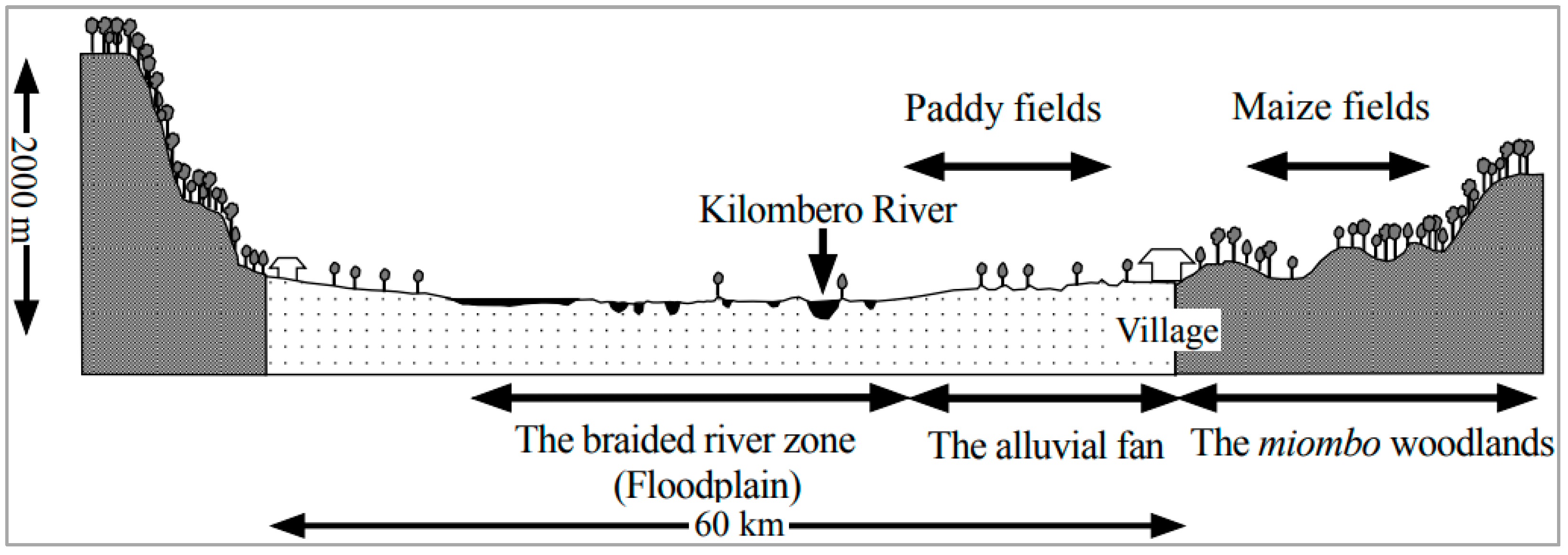
The current assessment focused on the hydrologic boundaries of the Kilombero River Catchment (Figure 1), which is part of Tanzania’s largest hydrologic basin, the Rufiji River Basin (RRB), spreading across 177,420 km2 (about 20% of Tanzania’s land mass). Kilombero River catchment in particular extends between longitudes 34°00′ E–37°20′ E and latitudes 07°40′ S–10°00′ S and covers an area of approximately 40,000 km2 [33]. The cross-section of the catchment (Figure 2) is characteristic of a graben structure, with the Udzungwa mountain ranges and Mbarika escarpments forming the northerly and southerly crests, respectively, while the middle part (the flood plain) forming the trough extending around 1967 km2 [39,40]. This middle part constitutes one of the largest wetlands in East Africa, i.e., Kibasira wetland, which is at around 300 m above mean sea level [41], and most of its area is internationally designated as a Ramsar site for its environmental significance [42]. Kilombero River catchment is the most important catchment with respect to agriculture, energy production, natural resources, and flow to RRB [42]. Tributaries contributing to the Kilombero River catchment are Lumemo, Luipa, Mngeta, Kihansi, Mpanga, Mnyela, Ruhuji, and Furua. Most areas of KRC are situated in the administrative region of Morogoro, where its most developed center (Ifakara) is found some 400 km from Dar es Salaam.

2.2. Methods

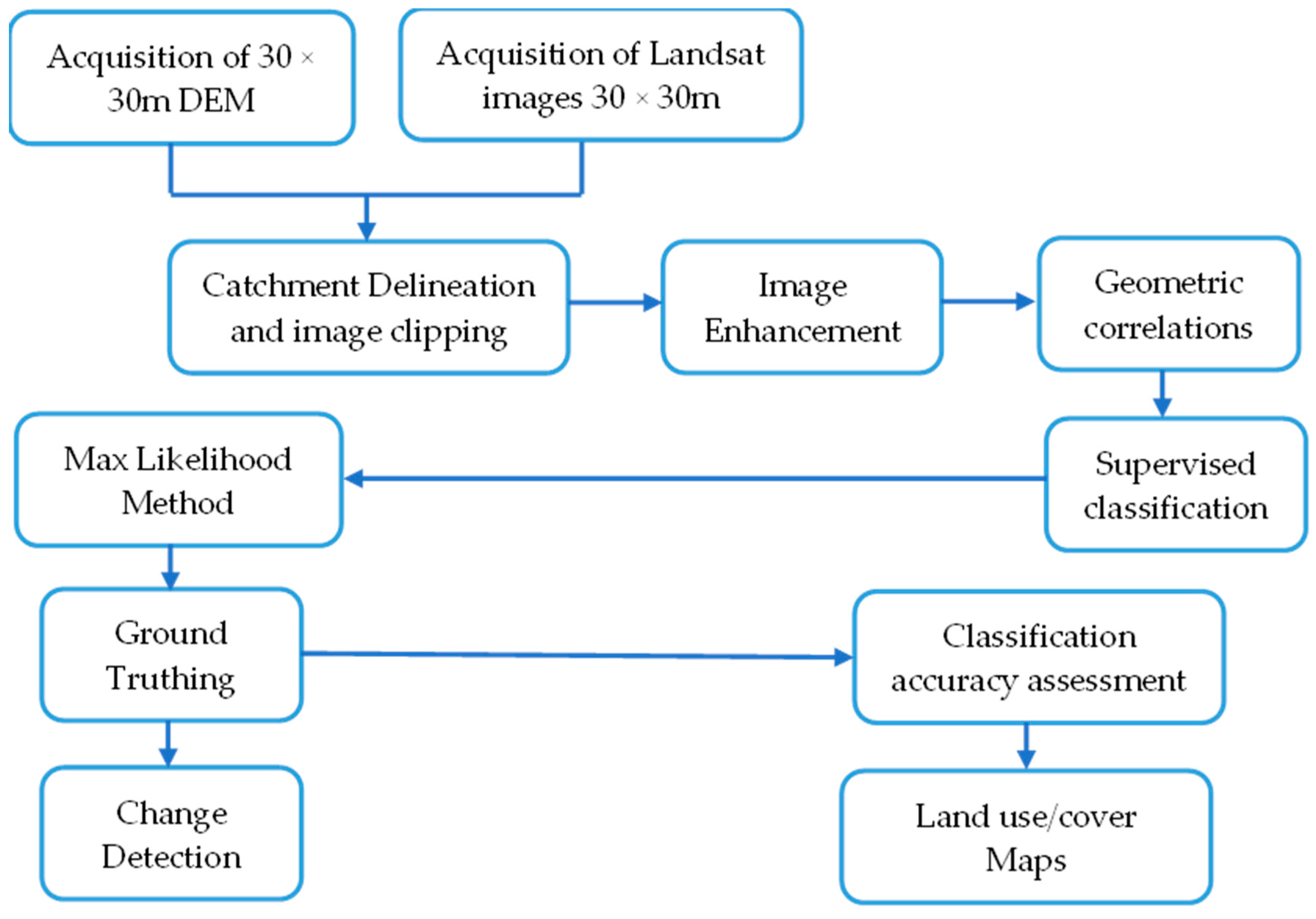
The study employed GIS and RS techniques to carry out land use/cover assessments. This started with the acquisition of geospatial data and subsequent image processing and analysis. Figure 3 below shows a methodological chart to simplify visualization of the process undertaken in this study.

2.3. Data Acquisition

Spatial and temporal land use/land cover transformations for KRC were detected for four time epochs (1991, 2001, 2011, and 2021) based on the analysis of remote sensing Landsat imagery and GIS. The selection of time epochs was meant to coincide with changes in national water policies since their first promulgation in 1991. Appropriate Landsat imageries were acquired from the United States Geological Survey (https://earthexplorer.usgs.gov/ accessed on 3 November 2022), i.e., 30 m resolution, multispectral level-2 data with cloud cover less than 10% (Table 1). These were accessed free of charge and proved by other scholars to have had excellent results [43,44], although higher-resolution images are in existence. Field observations were made prior to image classification to establish accurate locational point data for each land use/land cover class included in the classification. During ground truthing, a total of eight (8) major land use/land covers were identified, which are forest, woodland, bushland, grassland, water bodies, wetland, cultivated land, and built-up areas (Table 2).

2.4. Image Pre-Processing and Classification

Images were geometrically rectified to ensure geometric compatibility and registered to the UTM map coordinate system, UTM zone 37 South, Spheroid Clarke 1880, Datum Arc 1960. An image mosaic was conducted to merge together images of the same year with the same path and different rows so as to create a single image that covers the entire cluster. The unsupervised image classification using the k-means clustering algorithm was conducted for all images using ERDAS IMAGINE. The k-means algorithm partitions the data into k distinct, non-overlapping clusters based on the similarity of the data points, which helps reduce intra-class variability and enhance the separability between different land cover classes. A maximum of thirty-six (36) land use/land cover classes were formulated. The formulated classes were visually interpreted and confirmed through the use of ground-truth data and hybrid Google Maps. Similar classes were joined and re-coded into general classes based on the classification scheme established during ground truthing (Table 2).
The selection of image processing techniques needed careful consideration of the balance between interpretability and performance [45,46]. The traditional method yields results that are more easily interpretable, facilitating a better understanding of the contributions made by different features in the decision-making process. This advantage is particularly pronounced when dealing with small datasets, as modern techniques typically necessitate a substantial amount of labeled data for effective training [46]. In the case of a small dataset, it is often recommended to employ traditional approaches in order to minimize the likelihood of overfitting the model [45,46]. Therefore, due to the limited dataset in the study area, this study was performed using a hybrid of supervised and unsupervised image classification techniques.

2.5. Accuracy Assessment and Change Detection Analysis

The study applied users’ and producers’ accuracies to conduct a cross-tabulation between the class values and the ground truth, which resulted in an error matrix. To find out how accurate the classification was, the non-parametric kappa coefficient statistics were used to assess the accuracy of the final classified image (Equation (1)) by looking at the diagonal elements in the confusion matrix [47]. The authors adopted the use of kappa statistics as one of the best-applied accuracy assessment tests performed in many studies across the region [48,49,50,51]. Furthermore, it is now widely used as a chance-corrected measure of nominal agreement in a variety of application areas [52,53]. In the context of interobserver agreement studies, different scholars have persuaded the scientific world in favor of the usability of this statistic over other measures of agreement that have been proposed [53]. However, there are occasional limitations where the percentage of observer agreement may be high while the kappa coefficient is agreeably low [53]. As such, the assessment of correctness involved the utilization of 90 pixels per category, based on both visual interpretation and ground truth data. The reference data utilized for ground-truthing purposes was acquired from a high-resolution Google Earth platform as well as through a field visit that involved the use of GPS technology. Additionally, previously classified land use and land cover (LULC) data were also employed in this study.
K = N   i = 1 r x i i     i = 1 r ( x i + × x + i ) N 2 i = 1 r ( x i + × x + i )
where N is the total number of sites in the matrix, r is the number of rows in the matrix, xii is the number in row i and column i, x+i is the total for row i, and xi+ is the total for column.
Change detection analysis was conducted to quantify the extent, rate, and location of changes in land use between different time epochs. The study used post-classification comparisons to assess land use and land cover changes. The approach identifies changes by comparing independently classified multi-date images pixel-by-pixel using a change-detection matrix [54]. The estimation for the rate of change for the different land covers was computed based on [55].

2.6. Predicting Future Land Use/Land Cover Change

Cellular automata and Markov chain (CA-Markov) analysis were used to predict the spatial distribution of land use/land cover in the future. Classified land use/land cover maps for 2011, which represent the past, and 2021, which represent the current, were used to generate conditional transition probabilities (Table 3), which were later used to simulate land use/land cover for 2031 and 2041. The Markov chain is a statistical tool that describes the probability of land use/land cover changing from one time period to another by developing a transitional probability matrix between the first period and second period based on the spatial neighborhood effects [56,57,58]. The spatial neighborhood effect is the ability of neighboring cells to influence the transition of a given cell into different states [27]. This model was based on using and evaluating land use/land cover layers from previous years to predict the spatial distribution of land use/land cover in the future [59]. CA, on the other hand, is a collection of cells arranged in a grid of a specified shape, such that each cell changes state as a function of time, according to a defined set of rules driven by the states of neighboring cells [60]. CAs have been suggested for possible use in public key cryptography, as well as for applications in geography, anthropology, political science, sociology, and physics, among others. CA are useful because they are much simpler than complex mathematical equations but produce results that are more complex; they can be modeled using precise results (degree of closeness with real-world systems), and CA can mimic the actions of any possible physical system [61]. For better simulation of temporal and spatial patterns of land use/land cover changes in quantity and space, a combination of two techniques—Markov chain analysis and cellular automata (CA-Markov)—was used.

2.7. CA-Markov Model Set-Up and Validation

The simulated model was developed using IDRISI Selva v.17.0 software [62]. In the developing CA Markov model, the classified land use maps of 2011, representing the past, and 2021, representing the present, developed in QGIS 2.12.1 were converted into IDRISI data format and selected to be input data into the model to calculate matrices of conversion probabilities and conversion areas (transition area matrix and transition probability matrix). For model validation, the simulated land use/cover map for 2021 was compared with the actual satellite-derived land use/cover map based on kappa statistics. Then, a standard kappa index was used to assess whether the model was valid or not (usually the kappa index for a valid model is >70%) [63]. If the model has a kappa index of less than 70%, then the suitability map for the land covers and filter used should be repeated based on several considerations.

3. Results

3.1. Accuracy Assessment

Table 4 shows the producer’s accuracy (PA), user’s accuracy (UA), overall accuracies, and kappa statistics of the various land use/land cover classes in the Kilombero River catchment maps for different periods. The overall land use/land cover classification accuracy for the years 1991, 2001, 2011, and 2021 is 92.01%, 91.74%, 91.96%, and 92.44%, respectively, with an overall kappa statistics of 0.90 for all years. The accuracy results show good agreement, which is acceptable for the classification, detection, and prediction of land use/land cover in the Kilombero River catchment [64,65,66].

3.2. Historical Land use/Land Cover Change Pattern

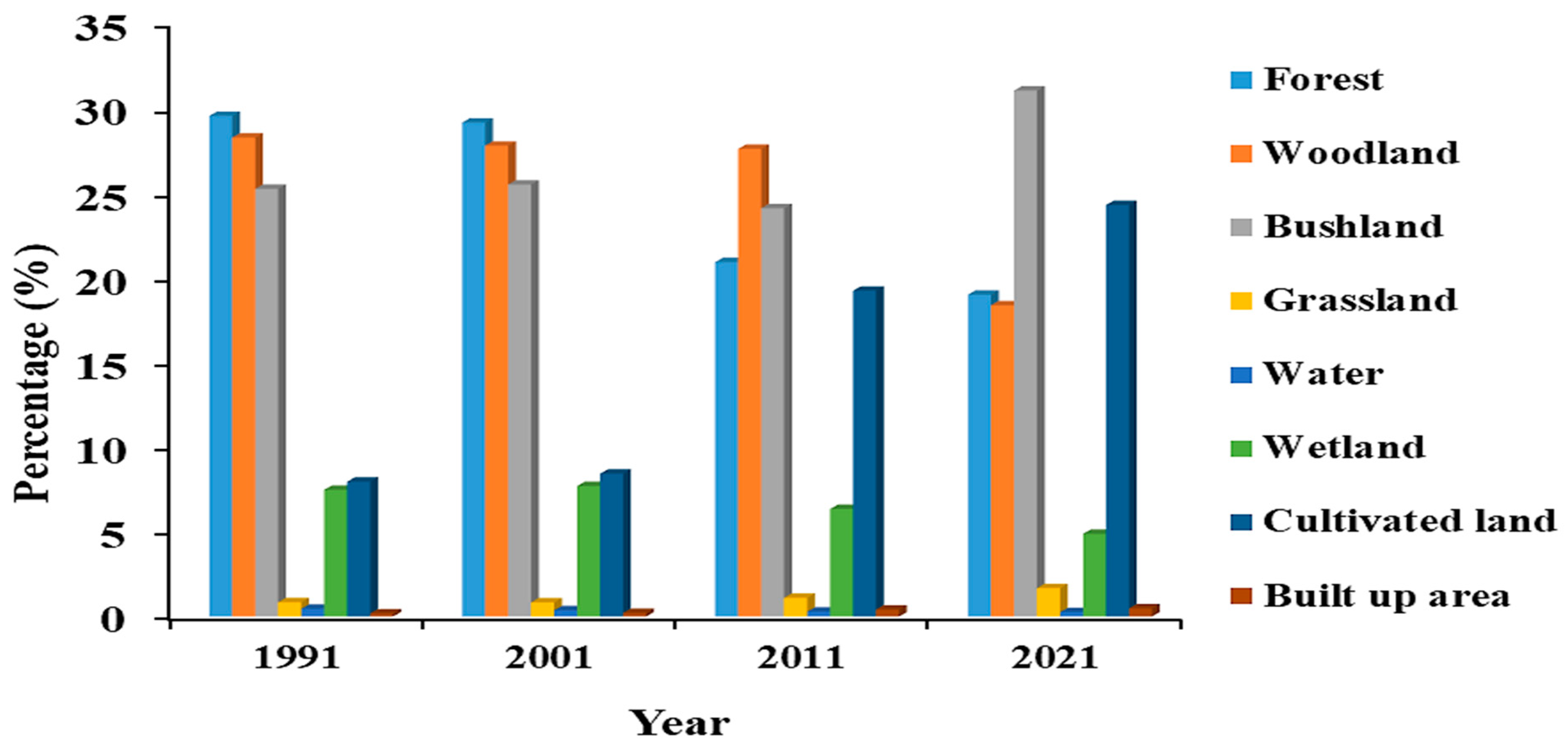
The areas under different land use/land cover types and percentages are given in Table 5. The land use/land cover percentage graphs and maps for the years 1991, 2001, 2011, and 2021 are presented in Figure 4 and Figure 5, respectively. Table 5 shows that land use/land cover for the year 1991 was dominated by forest (1,192,996 Ha) followed by woodland (1,141,382 Ha), bushland (1,019,128 Ha), cultivated land (321,188 Ha), wetland (302,098 Ha), grassland (34,067 Ha), water (18,641 Ha), and built-up area (7437 Ha). For the year 2001, land use/land cover was dominated by forest (1,177,109 Ha), woodland (1,121,891 Ha), bushland (1,029,224 Ha), cultivated land (340,472 Ha), wetland (311,029 Ha), grassland (33,500 Ha), water (15,075 Ha), and built-up area (8615 Ha). Moreover, the dominant land use/land cover for the year 2011 was woodland (1,114,763 Ha), followed by bushland (972,794 Ha), forest (844,527 Ha), cultivated land (776,118 Ha), wetland (256,250 Ha), grassland (44,310 Ha), built-up area (19,331 Ha), and water (11,578 Ha). For the last year of the study period, i.e., 2021, the dominant land use/land cover was bushland (1,253,491 Ha) followed by cultivated land (980,534 Ha), forest (766,835 Ha), woodland (714,798 Ha), wetland (196,912 Ha), grassland (67,614 Ha), built-up area (19,331 Ha), and water (10,419 Ha).
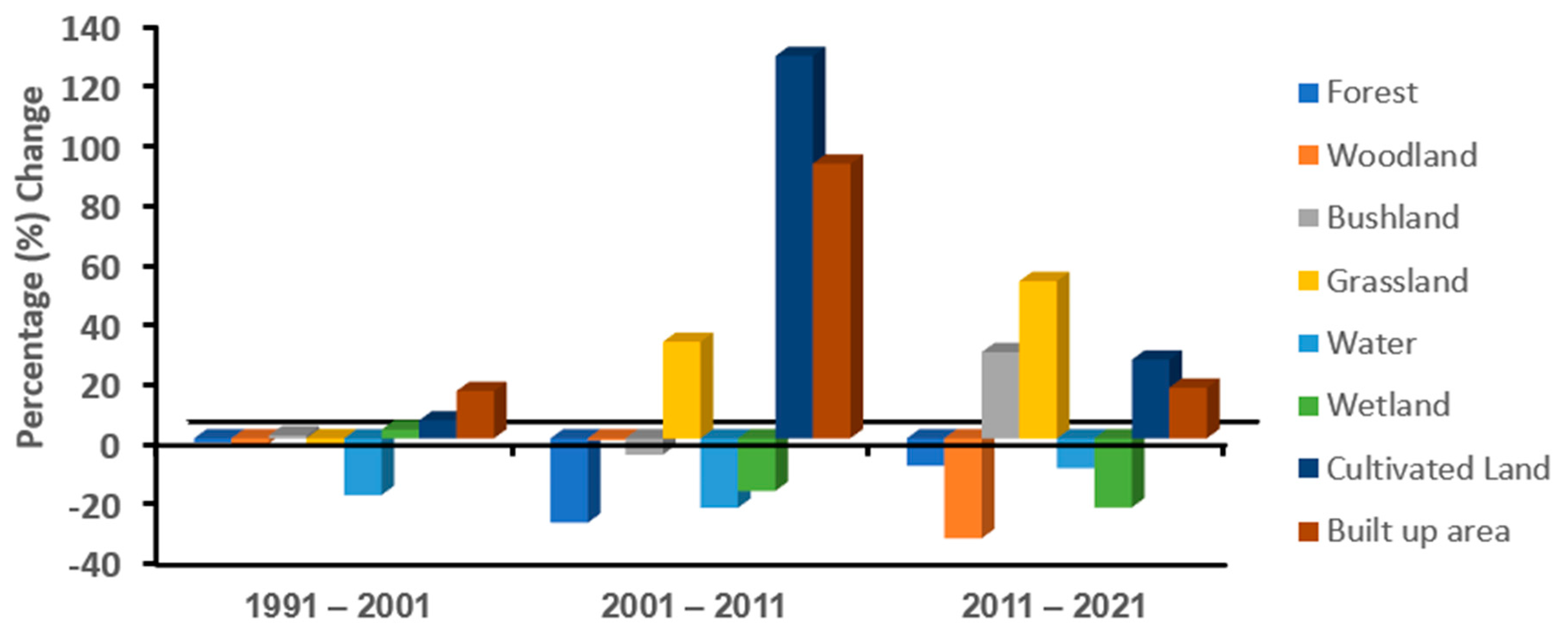
The changes in land use/land cover for the study periods of 1991–2001, 2001–2011, and 2011–2021 are given in Table 6 and illustrated in Figure 5 and Figure 6. During the study period 1991–2001, woodland experienced a maximum decrease of 19,492 Ha, followed by forest (15,887 Ha), water (3546 Ha), and grassland (567 Ha), while a maximum increase was observed in cultivated land (19,284 Ha), followed by bushland (10,096 Ha), wetland (8932 Ha), and built-up area (1179 Ha). The maximum annual decrease was observed in woodland (1949 Ha), followed by forest (1589 Ha), water (355 Ha), and grassland (57 Ha), while the maximum annual increase was observed in cultivated land (1928 Ha), followed by bushland (1010 Ha), wetland (893 Ha), and built-up area (118 Ha). During the study period 2001–2011, the results showed an increase in cultivated land (435,710 Ha), grassland (10,810 Ha), and built-up area (7916 Ha), while a decrease was observed in forest (332,582 Ha), bushland (56,430 Ha), wetland (54,779 Ha), woodland (7128 Ha), and water (3517 Ha). Furthermore, a maximum annual decrease was observed in forest (33,258 Ha), followed by bushland (5643 Ha), wetland (5478 Ha), woodland (713 Ha), and water (352 Ha), while a maximum annual increase was observed in cultivated land (43,571 Ha), grassland (1081 Ha), and built-up area (792 Ha). During the study period 2011–2021, a maximum increase was observed in bushland (280,698 Ha), followed by cultivated land (204,353 Ha), grassland (23,304 Ha), and built-up area (2800 Ha), while a maximum decrease was observed in woodland (372,965 Ha), followed by forest (77,692 Ha), wetland (59,338 Ha), and water (1159 Ha). Moreover, a maximum annual decrease was observed in woodland (37,297 Ha), followed by forest (7769 Ha), wetland (5934 Ha), and water (116 Ha), while a maximum annual increase was observed in bushland (28,070 Ha), followed by cultivated land (20,435 Ha), grassland (2330 Ha), and built-up area (280 Ha).

3.3. Land Use/Land Cover Change Detection Matrix

Table 7, Table 8, Table 9 and Table 10 indicate the areas changed based on the change matrix cross-tabulation from 1991 to 2021, whereby the land use/land cover classes are compared to one another. For the study period between 1991 and 2021 (Table 7), among all the land use/land cover types, the forest experienced a maximum net loss (−426,123 Ha), followed by woodland (−399,615 Ha), wetland (105,187 Ha), and water (−8220 Ha). On the other hand, cultivated land experiences maximum net gain (659,346 Ha), followed by bushland (234,373 Ha), grassland (33,547 Ha), and built-up area (11,879 Ha). During the study duration (1991–2021), the maximum amount of land under forest remained intact, i.e., 528,049 Ha. This is followed by bushland (442,391 Ha), woodland (398,012 Ha), cultivated land (241,550 Ha), wetland (170,230 Ha), grassland (16,796 Ha), water (8596 Ha), and built-up area (5237 Ha). During the study period between 1991 and 2001, as summarized in Table 8, woodland experienced the most net loss (−19,491 Ha), followed by forest (−15,886 Ha), water (−3545 Ha), and grassland (−568 Ha). The land use/land cover that experienced a net gain in area was led by cultivated land (19,285 Ha), followed by bushland (10,095 Ha), wetland (8932 Ha), and lastly, built-up areas (1178 Ha). During the study duration (1991–2001), a total of 1,165,330 Ha of forest remained intact, followed by woodland (1,114,670 Ha), bushland (987,618 Ha), cultivated land (317,416 Ha), wetland (298,632 Ha), grassland (33,317 Ha), water (15,076 Ha), and built-up area (6893 Ha). Table 9 indicates the areas that changed based on the change matrix cross-tabulation from 2001 to 2011. According to this, cultivated land had experienced the most net gain (435,721 Ha), followed by grassland (10,809 Ha) and built-up areas (7915 Ha). Furthermore, forests experienced the most net loss in land mass (−332,574 Ha), followed by bushland (−56,430 Ha), wetland (−54,778 Ha), woodland (−7147 Ha), and water (−3516 Ha). During the same study period, the majority of area under woodland remained intact (830,707 Ha), followed by forest (742,548 Ha), bushland (684,154 Ha), cultivated land (288,257 Ha), wetland (234,274 Ha), grassland (33,500 Ha), water (10,058 Ha), and built-up area (8615 Ha). Table 10 shows the areas that changed based on the change matrix cross-tabulation from 2011 to 2021. The woodland experienced the most net loss (−372,978 Ha), followed by forests (−77,686 Ha), wetland (−59,339 Ha), and water (−1160 Ha). Furthermore, bushland experienced the largest net gain (280,699 Ha), followed by cultivated land (204,374 Ha), grassland (23,305 Ha), and built-up area (2785 Ha) During this study period, cultivated land had the largest area that remained intact (688,477 Ha), followed by bushland (592,540 Ha), forest (558,295 Ha), woodland (460,304 Ha), wetland (189,978 Ha), grassland (17,439 Ha), built-up area (12,511 Ha), and water (9112 Ha).

3.4. Future Land Use/Land Cover Simulation for 2031 and 2041

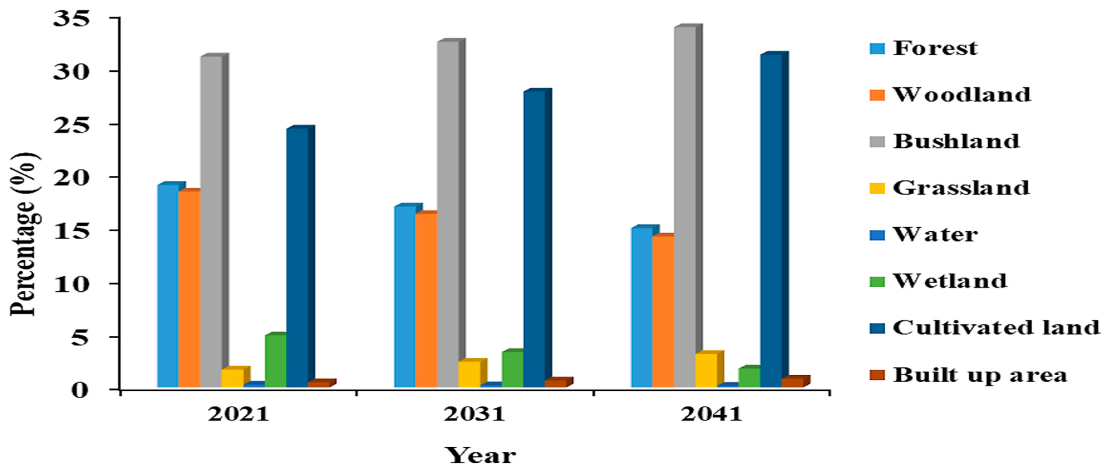
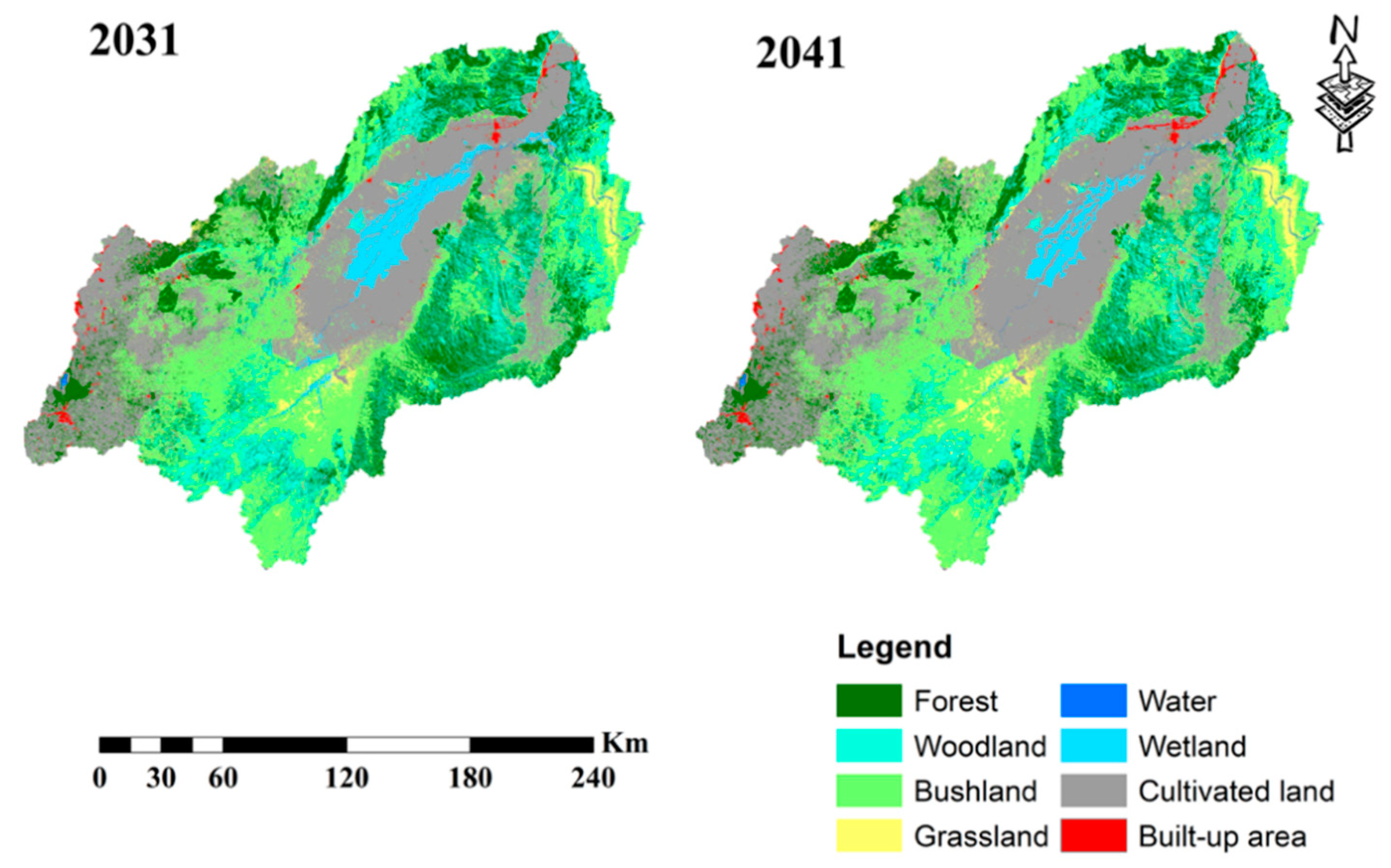
The validation target, the kappa index of agreement (KIA), was used for the 2021 land use/land cover predictions, which were acceptable to both the actual and the predicted land use/land cover. All the kappa results showed an acceptable standard greater than 80%, which confirmed that the prediction accuracy was reasonable for future land use/land cover prediction. The kappa statistics were as follows: Kno is 0.93, Klocation is 0.95, Kstrata is 0.95, and Kstandard is 0.91. The corrected percentage for each type of land use/land cover was over 90%, so the model was satisfactory for making predictions for 2031 and 2041, respectively. The predicted areas of land under different land use/land cover types and percentages are given in Table 11. The respective land use/land cover for this projected period are presented in Figure 7 and Figure 8 below. Table 11 shows that land use/land cover for the projected year 2031 will be dominated by bushland (1,309,248 Ha) followed by cultivated land (1,120,396 Ha), forest (685,239 Ha), woodland (657,047 Ha), wetland (133,897 Ha), grassland (97,030 Ha), built-up area (25,918 Ha), and water (8159 Ha). For the projected year 2041, land use/land cover will be dominated by bushland (1,364,920 Ha), followed by cultivated land (1,260,186 Ha), forest (603,307 Ha), woodland (571,806 Ha), grassland (126,654 Ha), wetland (71,291 Ha), built-up area (32,742 Ha), and water (6028 Ha).
The projected changes in land use/land cover for the periods 2021–2031 and 2031–2041 are given in Table 12 and illustrated in Figure 9. It is expected that from 2021–2031, woodland will experience a maximum decrease of 84,751 Ha, followed by forest (81,596 Ha), wetland (63,015 Ha), and water (2260 Ha) while maximum increases will be observed on cultivated land (139,862 Ha), followed by bushland (55,757 Ha), grassland (29,416 Ha), and built-up area 6587 Ha). The maximum annual decrease is expected in woodland (8475 Ha), followed by forest (8160 Ha), wetland (6302 Ha), and water (226 Ha), while the maximum annual increase is expected in cultivated land (13,986 Ha), followed by bushland (5576 Ha), grassland (2942 Ha), and built-up area (659 Ha). Moreover, for the projected changes for the period 2031–2041, a maximum decrease is expected in woodland (85,241 Ha), followed by forest (81,931 Ha), wetland (62,606 Ha), and water (2131 Ha), while a maximum increase is expected in cultivated land (13,979 Ha) followed by bushland (55,672 Ha), grassland (29,624 Ha) and built-up area (6824 Ha). The maximum annual decrease is expected in woodland (8524 Ha), followed by forest (8193 Ha) and wetland (6261 Ha), while a maximum annual increase is expected in cultivated land (13,979 Ha), followed by bushland (5567 Ha), grassland (2962 Ha), and built-up area (682 Ha).

4. Discussion

The assessment of LULC for this paper considered four time epochs, i.e., 1991, 2001, 2011, and 2021. We have also projected the same for the next two decades, i.e., 2031 and 2041. The selected time epochs were meant to coincide well with the national population census, whose growth contributes to most of the LULC changes. Furthermore, the results of the national census trigger major policy changes, e.g., the national water policy (NAWAPO) that was first promulgated in 1991, followed by 2002 [67], and the current drafting that started around 2022 and coincides with the population census of the same year. The projections were meant to coincide with the 2030 global and African targets, i.e., the sustainable development goals (SDG) [68] and the African forest landscape restoration initiative (AFR100), which is a country-led effort to bring 100 million Ha of land in Africa into restoration by 2030 [69,70]. Across the time epochs, the LULC classification accuracy was above 90%, whereas kappa statistics was 0.90, which shows high agreement and is hence acceptable for the classification, detection, and prediction of land use/land cover [64,65,66].
Analysis of LULC for each of the study years shows a growing transformation from domination of forests, woodland, and bushland to bushland and cultivated land as the top dominant LULC from 1991 to 2021 and as projected to 2031 and 2041. Considering that bushlands are essentially abandoned farmlands due to the occasional implementation of conservation policies and flooded farms [71,72], it means cultivated land has the most overall growing dominance in the study area. Furthermore, results show more shrinking landmass under wetland and water, which raises a red flag on water availability in the catchment. However, a parallel study by the authors [73] shows a diametric result (i.e., a consistent increase in water discharge at a rate of 498.6 m3/s/year) at the most downstream gauge station, i.e., Kilombero at Swero (1KB17), which is located in the protected Selous game reserve. This can be explained by either the fact that all hydroclimatic parameters show a favorable trend, as discussed in [73], or that changing LULC generated more sediment that has altered the cross-section of the more or less abandoned gauge station due to budget and accessibility through the game reserve (observed data between 29 November 1957 and 31 December 1981). Otherwise, the huge growing dominance of cultivated land would have caused a declining trend of water discharge at this strategic gauge station. With this in mind, along with the vast knowledge of what impacts are brought about by expansions in cultivation and settlements, it is safe to expect negative impacts on the downstream river flow regime (with natural high and low floods necessary for breeding [74,75]), its ecosystem service (e.g., the largest East African mangrove forest further downstream) [36,37,38], and economic flagship projects, i.e., Nyerere HEP. Furthermore, all these are expected to negatively impact the micro economy as local livelihoods depend directly on catchment ecosystem services, e.g., farming, fishing, weaving, etc. [41,76]. In addition, the macro economy may also be impacted given that the catchment is critical for national food production through expansion in SAGCOT as the Kilombero cluster [28,29] and the major HEP immediately downstream [35].
In addition, the conversion of LULC to more cultivated land creates loose soils that are swept by floods, meaning soil and water quality is changed. This is due to the known detrimental effects of agricultural practices on soil quality, which include erosion, desertification, salinization, compaction, and pollution [77]. On the other hand, farm inputs cause eutrophication, which ultimately leads to the reduction of oxygen in water and the release and accumulation of toxic substances in water and sediments, polluting the aquatic environment, which can lead to the death of aquatic organisms, ecosystems, and humans that may inadvertently drink or be exposed to the polluted water [78,79].
This study also studied the specific alteration of LULC from one such LULC to another. This is based on a change matrix cross-tabulation across the time epoch. The same shows that in the time span of 1991–2001, 2001–2011, 2011–2021, and overall, 1991–2021, forests and woodland lost the most landmass as compared to cultivated land and bushland that have gained the most. Although there was a consistent increase in land mass under cultivation, the period between 2001 and 2011 experienced the most significant jump. This could be attributed to three major government policies, i.e., the Big Results Now (BRN) of 2013, the Kilimo Kwanza Initiative (KKI), translated as the prioritization of agriculture in June 2009, and the establishment of the southern agricultural growth corridor (SAGCOT) by 2010. All of them are based on the need to link the local peasantry farmers with agribusiness actors across the corridor (including Kilombero, which forms the most consequential cluster). Furthermore, the privatization and establishment of big sugarcane, which Kilombero Sugar Company Limited (KSCL) took over in 1998, expanded significantly around 2005–2006 following their initiative to build the Kidatu Bridge and associated road improvements, which also spearheaded agriculture expansion in the catchment. In addition, Kilombero Plantations Limited (KPL) was privatized and expanded paddy farming activities by 2008–2010. Both plantations introduced and supported grower farmers, who expanded just as much as the plantations themselves. However, the implementation of the recently enacted Water Resources Management Act No. 11 of 2009 and the establishment of a record number of water users’ associations (WUA) in the catchment saw the decline of cultivated land within the protected wetland and river buffer. This increased bushland (abandoned farms) and reduced the declination of areas occupied by water. Wetland continued to decline since abandoned farms (bushlands) were yet to rejuvenate into proper wetlands.

5. Conclusions

This study has carried out LULC assessment and its implications for water availability in the Kilomebro River catchment (KRC). The former considered four time epochs, viz., 1991, 2001, 2011, and 2021, and were then projected into two subsequent decades, i.e., 2031 and 2041. These were pegged against the key drivers or targets nationally to regionally/globally. The assessment has demonstrated the LULC transformation in KRC following major government policies and/or anthropogenic dynamics. This has shown an alarming growth rate of areas under cultivation vs shrinkage of land mass occupied by water and/or wetlands. However, the growth of the water-thirsty sector seems to not impact the water availability at the most downstream gauging station, i.e., Kilombero at Swero (1KB17). Nevertheless, this station is located in an undeveloped game reserve area whose station assessment is not frequent and has not been operational since 31 December 1981.
The assessment has also indicated a steeper LULC conversion to cultivated land in 2010, during which the government introduced major agricultural programs in the SAGCOT area, especially the Kilombero cluster. With the ongoing access infrastructure development and expansion plans in this cluster, more LULC conversion to cultivated land and settlements is expected, as indicated in the project’s future. This will inevitably impact water availability in the catchment and hence impact other water uses, especially the environment and government flagship projects, e.g., the Nyerere hydropower project downstream of the Kilombero River catchment, which contributes to more than 60% of flow.
The following recommendations are proposed from this assessment:
(a)
Develop and support the implementation of guidelines for participatory land use planning that are responsive to nature conservation but reflect the livelihood means of poor people.
(b)
Re-evaluate modern protection mechanisms vs traditional ones that are inculcated in the cultural norms of local people.
(c)
Reevaluation of the status of Swero (1KB17) gauging station cross-section to ascertain the credibility of the ratting curve and hence the discharge data generated from its stuff gauge reading.
(d)
Implement agroforest policy to obtain two objectives, i.e., conservation (land and water) and economic growth from agriculture, which is the main economic activity.
(e)
Evaluate the implementability and socio-economic impact of a 60 m buffer zone from any water source as required in the Water Resources Management Act No. 11 of 2009 and the National Environmental Management Act No. 20 of 2004.
(f)
Continuous capacity building for locals (through WUAs and other institutions) and participatory law enforcement embedding water and natural resources management.

Author Contributions

Conceptualization and methodology, O.Z.S., S.T. and N.A.C. formal analysis, investigation, resources, data curation, and writing—original draft preparation, O.Z.S., N.A.C. and M.F.M.; writing—review and editing, O.Z.S. and S.T.; study supervision J.R.S. and P.V. All authors have read and agreed to the published version of the manuscript.

Funding

Costs for data and ground truthing were covered by corresponding author.

Data Availability Statement

Publicly available datasets were analyzed in this study. This data can be found here: https://earthexplorer.usgs.gov/ accessed on 3 November 2022.

Conflicts of Interest

The authors declare no conflict of interest.

References

  1. Li, X.; Chen, G.; Liu, X.; Liang, X.; Wang, S.; Chen, Y.; Pei, F.; Xu, X. A new global land-use and land-cover change product at a 1-km resolution for 2010 to 2100 based on human--environment interactions. Ann. Am. Assoc. Geogr. 2017, 107, 1040–1059. [Google Scholar] [CrossRef]
  2. Turner, B.; Meyer, W.B.; Skole, D.L. Global land-use/land-cover change: Towards an integrated study. Ambio. Stock. 1994, 23, 91–95. [Google Scholar]
  3. Foley, J.A.; DeFries, R.; Asner, G.P.; Barford, C.; Bonan, G.; Carpenter, S.R.; Chapin, F.S.; Coe, M.T.; Daily, G.C.; Gibbs, H.K.; et al. Global consequences of land use. Science 2005, 309, 570–574. [Google Scholar] [CrossRef]
  4. Khan, I.; Javed, T.; Khan, A.; Lei, H.; Muhammad, I.; Ali, I.; Huo, X. Impact assessment of land use change on surface temperature and agricultural productivity in Peshawar-Pakistan. Environ. Sci. Pollut. Res. 2019, 26, 33076–33085. [Google Scholar] [CrossRef]
  5. Meyer, W.B.; Turner, B.L. Human population growth and global land-use/cover change. Annu. Rev. Ecol. Syst. 1992, 23, 39–61. [Google Scholar] [CrossRef]
  6. Liu, Y.; Wang, D.; Gao, J.; Deng, W. Land use/cover changes, the environment and water resources in Northeast China. Environ. Manag. 2005, 36, 691–701. [Google Scholar] [CrossRef]
  7. Liu, Y. Introduction to land use and rural sustainability in China. Land Use Policy 2018, 74, 1–4. [Google Scholar] [CrossRef]
  8. Lupo, F.; Reginster, I.; Lambin, E.F. Monitoring land-cover changes in West Africa with SPOT Vegetation: Impact of natural disasters in 1998–1999. Int. J. Remote Sens. 2001, 22, 2633–2639. [Google Scholar] [CrossRef]
  9. Mbungu, W.B.; Kashaigili, J.J. Assessing the hydrology of a data-scarce tropical watershed using the soil and water assessment tool: Case of the Little Ruaha River Watershed in Iringa, Tanzania. Open J. Mod. Hydrol. 2017, 7, 65–89. [Google Scholar] [CrossRef]
  10. Li, R.-Q.; Dong, M.; Cui, J.-Y.; Zhang, L.-L.; Cui, Q.-G.; He, W.-M. Quantification of the impact of land-use changes on ecosystem services: A case study in Pingbian County, China. Environ. Monit. Assess. 2007, 128, 503–510. [Google Scholar] [CrossRef]
  11. Näschen, K.; Diekkrüger, B.; Leemhuis, C.; Steinbach, S.; Seregina, L.S.; Thonfeld, F.; der Linden, R. Hydrological modeling in data-scarce catchments: The Kilombero floodplain in Tanzania. Water 2018, 10, 599. [Google Scholar] [CrossRef]
  12. Sun, S.; Wang, Y.; Liu, J.; Cai, H.; Wu, P.; Geng, Q.; Xu, L. Sustainability assessment of regional water resources under the DPSIR framework. J. Hydrol. 2016, 532, 140–148. [Google Scholar] [CrossRef]
  13. Guo, Y.; Tian, X.; Fang, G.; Xu, Y.-P. Many-objective optimization with improved shuffled frog leaping algorithm for inter-basin water transfers. Adv. Water Resour. 2020, 138, 103531. [Google Scholar] [CrossRef]
  14. Ma, R.; Li, Y.L.; Ji, A.D. Evaluation of spatial equilibrium status for the Yellow River basin based on comprehensive multi-index method. South North Water Transf. Water Sci. Technol. 2021, 2, 217–225. [Google Scholar]
  15. Hou, C.; Wen, Y.; Liu, X.; Dong, M. Impacts of regional water shortage information disclosure on public acceptance of recycled water—Evidences from China’s urban residents. J. Clean. Prod. 2021, 278, 123965. [Google Scholar] [CrossRef]
  16. Roozbahani, R.; Schreider, S.; Abbasi, B. Optimal water allocation through a multi-objective compromise between environmental, social, and economic preferences. Environ. Model. Softw. 2015, 64, 18–30. [Google Scholar] [CrossRef]
  17. Xu, J.; Lv, C.; Yao, L.; Hou, S. Intergenerational equity based optimal water allocation for sustainable development: A case study on the upper reaches of Minjiang River, China. J. Hydrol. 2019, 568, 835–848. [Google Scholar] [CrossRef]
  18. Zhang, Y.; Lu, Y.; Zhou, Q.; Wu, F. Optimal water allocation scheme based on trade-offs between economic and ecological water demands in the Heihe River Basin of Northwest China. Sci. Total Environ. 2020, 703, 134958. [Google Scholar] [CrossRef]
  19. Huang, Y.; Cai, Y.; Xie, Y.; Zhang, F.; He, Y.; Zhang, P.; Li, B.; Li, B.; Jia, Q.; Wang, Y.; et al. An optimization model for water resources allocation in Dongjiang River Basin of Guangdong-Hong Kong-Macao Greater Bay Area under multiple complexities. Sci. Total Environ. 2022, 820, 153198. [Google Scholar] [CrossRef]
  20. Lambin, E.F.; Turner, B.L.; Geist, H.J.; Agbola, S.B.; Angelsen, A.; Bruce, J.W.; Coomes, O.T.; Dirzo, R.; Fischer, G.; Folke, C.; et al. The causes of land-use and land-cover change: Moving beyond the myths. Glob. Environ. Chang. 2001, 11, 261–269. [Google Scholar] [CrossRef]
  21. Munishi-Kongo, S. Ground and Satellite-Based Assessment of Hydrological Responses to Land Cover Change in the Kilombero River Basin, Tanzania. Ph.D. Thesis, University of KwaZulu-Natal, Durban, South Africa, 2013. [Google Scholar]
  22. Tumbo, M.; Hughes, D.A. Uncertain hydrological modelling: Application of the Pitman model in the Great Ruaha River basin, Tanzania. Hydrol. Sci. J. 2015, 60, 2047–2061. [Google Scholar] [CrossRef]
  23. Ritchie, J.C.; Zimba, P.V.; Everitt, J.H. Remote sensing techniques to assess water quality. Photogramm. Eng. Remote Sens. 2003, 69, 695–704. [Google Scholar] [CrossRef]
  24. Cetin, M.; Aksoy, T.; Cabuk, S.N.; Kurkcuoglu, M.A.S.; Cabuk, A. Employing remote sensing technique to monitor the influence of newly established universities in creating an urban development process on the respective cities. Land Use Policy 2021, 109, 105705. [Google Scholar] [CrossRef]
  25. Goodchild, M.F. A GIScience perspective on the uncertainty of context. Ann. Am. Assoc. Geogr. 2018, 108, 1476–1481. [Google Scholar] [CrossRef]
  26. Lü, G.; Batty, M.; Strobl, J.; Lin, H.; Zhu, A.-X.; Chen, M. Reflections and speculations on the progress in Geographic Information Systems (GIS): A geographic perspective. Int. J. Geogr. Inf. Sci. 2019, 33, 346–367. [Google Scholar] [CrossRef]
  27. Chilagane, N.A.; Kashaigili, J.J.; Mutayoba, E. Historical and future spatial and temporal changes in land use and land cover in the little Ruaha River catchment, Tanzania. J. Geosci. Environ. Prot. 2020, 8, 76–96. [Google Scholar] [CrossRef]
  28. Milder, J.C.; Hart, A.; Buck, L.E. Applying an Agriculture Green Growth Approach in the SAGCOT Clusters: Challenges and Opportunities in Kilombero, Ihemi and Mbarali; SAGCOT Center: Dar Es Salaam, Tanzania, 2013. [Google Scholar]
  29. Buck, L.; Milder, J. SAGCOT Green Growth Leaders Workshop Report; SAGCOT Center Ltd.: Dar Es Salaam, Tanzania, 2012; 61p. [Google Scholar]
  30. Mutayoba, E.; Kashaigili, J.J.; Kahimba, F.C.; Mbungu, W.; Chilagane, N.A. Assessing the impacts of land use and land cover changes on hydrology of the Mbarali River Sub-Catchment. The Case of Upper Great Ruaha Sub-Basin, Tanzania. Engineering 2018, 10, 616. [Google Scholar] [CrossRef]
  31. Twisa, S.; Buchroithner, M.F. Land-use and land-cover (LULC) change detection in Wami River Basin, Tanzania. Land 2019, 8, 136. [Google Scholar] [CrossRef]
  32. Twisa, S.; Mwabumba, M.; Kurian, M.; Buchroithner, M.F. Impact of land-use/land-cover change on drinking water ecosystem services in Wami River Basin, Tanzania. Resources 2020, 9, 37. [Google Scholar] [CrossRef]
  33. WREM International Inc. WREM & RBWB Rufiji Basin Integrated Water Resources Management and Development Plan Draft Final Report. Volume 1: Rufiji Basin Plan. Report Prepared for the United Republic of Tanzania; Ministry of Water: Atlanta, GA, USA, 2013; p. 11.
  34. WREM International Inc. WREM & RBWB Rufiji IWRMD Plan Draft Final Report. Volume 1: Climate and Hydrologic Modeling and Assessments. Report Prepared for the United Republic of Tanzania; Ministry of Water: Atlanta, GA, USA, 2013.
  35. Dye, B.; Hartmann, J. The True Cost of Power: The Facts and Risks of Building the Stiegler’s Gorge Hydropower Dam in the Selous Game Reserve, Tanzania; The University of Manchester: Manchester, UK, 2017. [Google Scholar]
  36. Monga, E.; Mangora, M.M.; Mayunga, J.S. Mangrove cover change detection in the Rufiji Delta in Tanzania. West. Indian Ocean J. Mar. Sci. 2018, 17, 1–10. [Google Scholar] [CrossRef]
  37. Ajonina, G.; Diamé, A.; Kairo, J. Current status and conservation of mangroves in Africa: An overview. World Rainfor. Mov. Bull. 2008, 133, 1–6. [Google Scholar]
  38. Mangora, M.M.; Shalli, M.S.; Semesi, I.S.; Njana, M.A.; Mwainunu, E.J.; Otieno, J.E.; Ntibasubile, E.; Mallya, H.C.; Mukama, K.; Wambura, M.; et al. Designing a mangrove research and demonstration forest in the rufiji delta, Tanzania. In Proceedings of the 5th Interagency Conference on Research in the Watersheds, Amherst, MA, USA, 9–11 September 2016; pp. 190–192. [Google Scholar]
  39. Kato, F. Development of a major rice cultivation area in the Kilombero Valley, Tanzania. Afr. Study Monogr. Suppl. Issue. 2007, 36, 3–18. [Google Scholar]
  40. Mombo, F.; Speelman, S.; Huylenbroeck, G.; Van Hella, J.; Pantaleo, M. Ratification of the Ramsar convention and sustainable wetlands management: Situation analysis of the Kilombero Valley wetlands in Tanzania. J. Agric. Ext. Rural. Dev. 2011, 3, 153–164. [Google Scholar]
  41. Kangalawe, R.Y.M.; Liwenga, E.T. Livelihoods in the wetlands of Kilombero Valley in Tanzania: Opportunities and challenges to integrated water resource management. Phys. Chem. Earth Parts A/B/C 2005, 30, 968–975. [Google Scholar] [CrossRef]
  42. Wilson, E.; McInnes, R.; Mbaga, D.P.; Ouedraogo, P. Kilombero Valley, United Republic of Tanzania: Ramsar Advisory Mission Report; Ramsar Site No. 1173; Ramsar Site: Ramsar, Iran, 2017. [Google Scholar]
  43. Zhang, Y.; Woodcock, C.E.; Arévalo, P.; Olofsson, P.; Tang, X.; Stanimirova, R.; Bullock, E.; Tarrio, K.R.; Zhu, Z.; Friedl, M.A. A global analysis of the spatial and temporal variability of usable Landsat observations at the pixel scale. Front. Remote Sens. 2022, 3, 894618. [Google Scholar] [CrossRef]
  44. Kovalskyy, V.; Roy, D.P. The global availability of Landsat 5 TM and Landsat 7 ETM+ land surface observations and implications for global 30 m Landsat data product generation. Remote Sens. Environ. 2013, 130, 280–293. [Google Scholar] [CrossRef]
  45. Doshi-Velez, F.; Kim, B. Towards a rigorous science of interpretable machine learning. arXiv 2017, arXiv:1702.08608. [Google Scholar]
  46. Sarker, I.H. Machine learning: Algorithms, real-world applications and research directions. SN Comput. Sci. 2021, 2, 160. [Google Scholar] [CrossRef]
  47. Rosenfield, G.H.; Fitzpatrick-Lins, K. A coefficient of agreement as a measure of thematic classification accuracy. Photogramm. Eng. Remote Sens. 1986, 52, 223–227. [Google Scholar]
  48. Larbi, I.; Forkuor, G.; Hountondji, F.C.C.; Agyare, W.A.; Mama, D. Predictive land use change under business-as-usual and afforestation scenarios in the vea catchment, West Africa. Int. J. Adv. Remote Sens. GIS 2019, 8, 3011–3029. [Google Scholar] [CrossRef]
  49. Gashaw, T.; Tulu, T.; Argaw, M.; Worqlul, A.W. Evaluation and prediction of land use/land cover changes in the Andassa watershed, Blue Nile Basin, Ethiopia. Environ. Syst. Res. 2017, 6, 17. [Google Scholar] [CrossRef]
  50. Gong, W.; Yuan, L.; Fan, W.; Stott, P. Analysis and simulation of land use spatial pattern in Harbin prefecture based on trajectories and cellular automata—Markov modelling. Int. J. Appl. Earth Obs. Geoinf. 2015, 34, 207–216. [Google Scholar] [CrossRef]
  51. Singh, S.K.; Mustak, S.; Srivastava, P.K.; Szabó, S.; Islam, T. Predicting spatial and decadal LULC changes through cellular automata Markov chain models using earth observation datasets and geo-information. Environ. Process. 2015, 2, 61–78. [Google Scholar] [CrossRef]
  52. Donner, A.; Klar, N. The statistical analysis of kappa statistics in multiple samples. J. Clin. Epidemiol. 1996, 49, 1053–1058. [Google Scholar] [CrossRef] [PubMed]
  53. Dettori, J.R.; Norvell, D.C. Kappa and beyond: Is there agreement? Glob. Spine J. 2020, 10, 499–501. [Google Scholar] [CrossRef] [PubMed]
  54. Kashaigili, J.J.; McCartney, M.; Mahoo, H.F.; Lankford, B.A.; Mbilinyi, B.P.; Yawson, D.K.; Tumbo, S.D. Use of a Hydrological Model for Environmental Management of the Usangu Wetlands, Tanzania; IWMI: Colombo, Sri Lanka, 2006; Volume 104. [Google Scholar]
  55. Kashaigili, J.J.; Majaliwa, A.M. Integrated assessment of land use and cover changes in the Malagarasi river catchment in Tanzania. Phys. Chem. Earth Parts A/B/C 2010, 35, 730–741. [Google Scholar] [CrossRef]
  56. Al-Bakri, J.T.; Duqqah, M.; Brewer, T. Application of remote sensing and GIS for modeling and assessment of land use/cover change in Amman/Jordan. J. Geogr. Inf. Syst. 2013, 2013, 38390. [Google Scholar] [CrossRef]
  57. Araya, Y.H.; Cabral, P. Analysis and modeling of urban land cover change in Setúbal and Sesimbra, Portugal. Remote Sens. 2010, 2, 1549–1563. [Google Scholar] [CrossRef]
  58. Wang, T.; Wu, W.; Xue, X. Spatial-temporal changes of sandy desertified land during last 5 decades in northern China. ACTA Geogr. Sin. Ed. 2004, 59, 203–212. [Google Scholar]
  59. Wu, N.; Silva, E.A. Artificial intelligence solutions for urban land dynamics: A review. J. Plan. Lit. 2010, 24, 246–265. [Google Scholar]
  60. Ghosh, P.; Mukhopadhyay, A.; Chanda, A.; Mondal, P.; Akhand, A.; Mukherjee, S.; Nayak, S.K.; Ghosh, S.; Mitra, D.; Ghosh, T.; et al. Application of Cellular automata and Markov-chain model in geospatial environmental modeling—A review. Remote Sens. Appl. Soc. Environ. 2017, 5, 64–77. [Google Scholar] [CrossRef]
  61. Silva, E.A. Cellular Automata and Agent Base Models for Urban Studies: From Pixels to Cells to Hexa-dpi’s. Urban Remote Sens. Monit. Synth. Model. Urban Environ. 2011, 250, 323–334. [Google Scholar]
  62. Rutherford, J.; Kobryn, H.; Newsome, D. A case study in the evaluation of geotourism potential through geographic information systems: Application in a geology-rich island tourism hotspot. Curr. Issues Tour. 2015, 18, 267–285. [Google Scholar] [CrossRef]
  63. Wen, W. Wetland Change Prediction Using Markov Cellular Automata Model in Lore Lindu National Park Central Sulawesi Province, Indonesia (Seminar); IPB University: Bogor, Indonesia, 2008. [Google Scholar]
  64. Anderson, J.R. A Land Use and Land Cover Classification System for Use with Remote Sensor Data; US Government Printing Office: Washington, DC, USA, 1976; Volume 964.
  65. Jensen, J.R. Digital Image Processing: A Remote Sensing Perspective; Prentice Hall: Upper Saddle River, NJ, USA, 2005. [Google Scholar]
  66. Lillesand, T.; Kiefer, R.W.; Chipman, J. Remote Sensing and Image Interpretation; John Wiley & Sons: Hoboken, NJ, USA, 2015. [Google Scholar]
  67. MoW The National Water Policy (NAWAPO). Ministry of Water under the Government of the United Republic of Tanzania; MoW The National Water Policy (NAWAPO): Dar es Salaam, Tanzania, 2002.
  68. United Nations (UN). The Seventeen (17) Sustainable Development Goals. Department of Economic and Social Affairs for Sustainable Development. Available online: https://sdgs.un.org/goals (accessed on 22 March 2021).
  69. Mansourian, S.; Berrahmouni, N.; Blaser, J.; Dudley, N.; Maginnis, S.; Mumba, M.; Vallauri, D. Reflecting on twenty years of forest landscape restoration. Restor. Ecol. 2021, 29, e13441. [Google Scholar] [CrossRef]
  70. Saint-Laurent, C.; Begeladze, S.; Vidal, A.; Hingorani, S. The Bonn Challenge: Building momentum on restoration. Unasylva 2020, 252, 82–91. [Google Scholar]
  71. Munishi, P.K.T.; Chuwa, J.J.; Kilungu, H.; Moe, S.R.; Temu, R.P.C. Management Effectiveness and Conservation Initiatives in the Kilombero Valley Flood Plains Ramsar Site, Tanzania. Tanzan. J. For. Nat. Conserv. 2012, 81, 1–10. [Google Scholar]
  72. Balama, C.; Augustino, S.; Eriksen, S.; Makonda, F.S.B.; Amanzi, N. Climate change adaptation strategies by local farmers in Kilombero District, Tanzania. Ethiop. J. Environ. Stud. Manag. 2013, 6, 724–736. [Google Scholar]
  73. Sigalla, O.Z.; Valimba, P.; Selemani, J.R.; Tumbo, M.H. Analysis of Spatial and Temporal Trend for Hydro-climatic Parameters in the Kilombero River Catchment, Tanzania. Sci. Rep. 2023, 13, 7864. [Google Scholar] [CrossRef]
  74. Duvail, S.; Hamerlynck, O. The Rufiji River flood: Plague or blessing? Int. J. Biometeorol. 2007, 52, 33–42. [Google Scholar] [CrossRef]
  75. Wagner, G.M.; Sallema-Mtui, R. The Rufiji Estuary: Climate change, anthropogenic pressures, vulnerability assessment and adaptive management strategies. In Estuaries: A Lifeline of Ecosystem Services in the Western Indian Ocean; Springer: Cham, Switzerland, 2016; pp. 183–207. [Google Scholar]
  76. Sigalla, O.Z.; Kadigi, R.M.J.; Komakech, H.C. Profitability Analysis of Paddy Farming Systems in Wetland Areas: An Additional Layer in Water Allocation Decisions. Curr. Res. Environ. Sustain. 2022, 14, 3459. [Google Scholar]
  77. Zalidis, G.; Stamatiadis, S.; Takavakoglou, V.; Eskridge, K.; Misopolinos, N. Impacts of agricultural practices on soil and water quality in the Mediterranean region and proposed assessment methodology. Agric. Ecosyst. Environ. 2002, 88, 137–146. [Google Scholar] [CrossRef]
  78. Rast, W.; Holland, M. Eutrophication of lakes and reservoirs: A framework for making management decisions. Ambio 1988, 17, 2–12. [Google Scholar]
  79. Downing, J.A.; Polasky, S.; Olmstead, S.M.; Newbold, S.C. Protecting local water quality has global benefits. Nat. Commun. 2021, 12, 2709. [Google Scholar] [CrossRef]
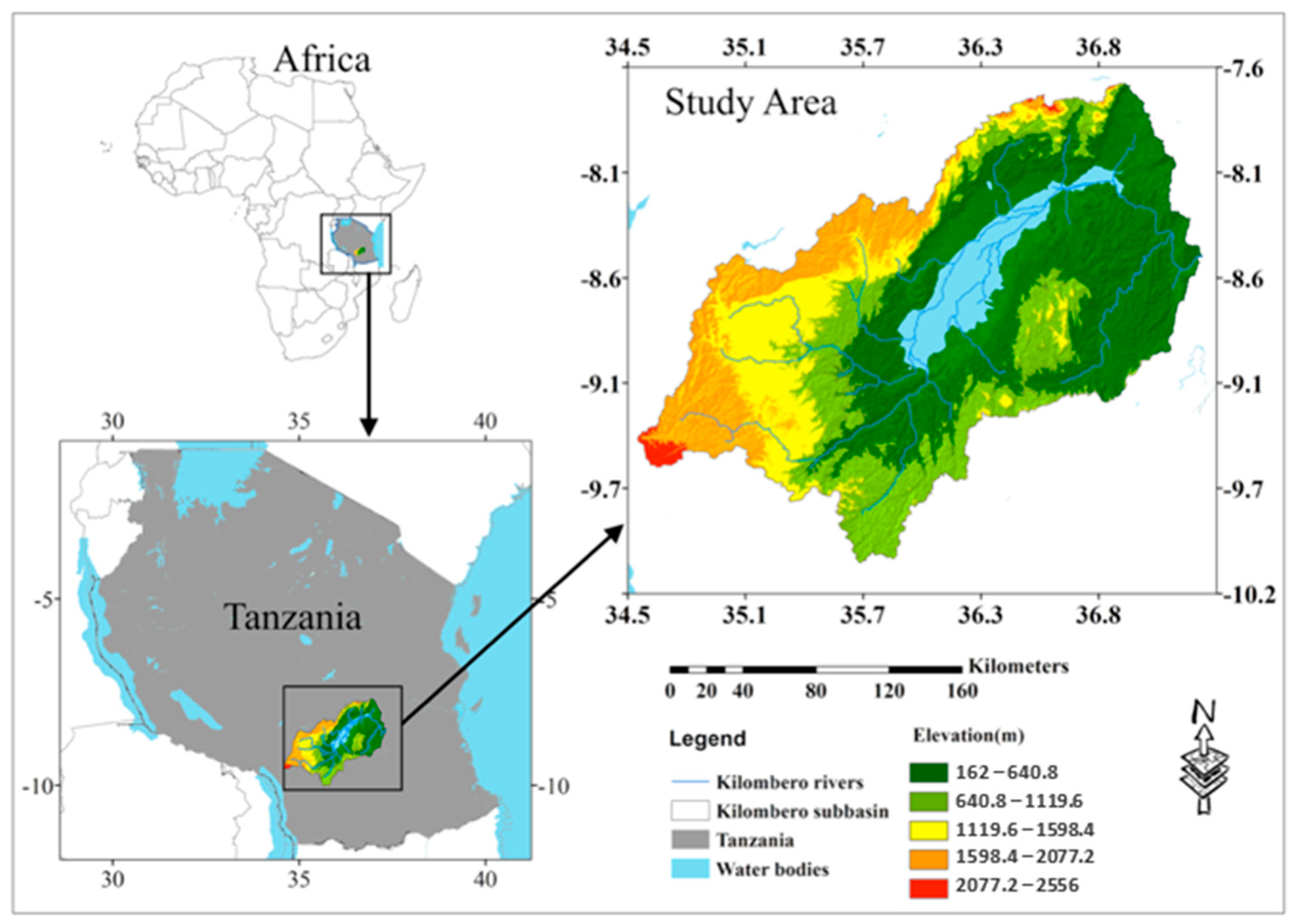
Figure 1. The study area of Kilombelo River catchment.
Water 16 00493 g001
Figure 2. The east–west cross-section of the Kilombero River catchment—adopted from [39].
Water 16 00493 g002
Figure 3. Methodological flow chart considered in this assessment.
Water 16 00493 g003
Figure 4. Land use/land cover graph for 1991, 2001, 2011, and 2021 at Kilombero River catchment.
Water 16 00493 g004
Figure 5. Land use/land cover maps for 1991, 2001, 2011, and 2021 at Kilombero River catchment.
Water 16 00493 g005
Figure 6. Historical land use/land cover changes for time span 1991–2001; 2001–2011; and 2011–2021.
Water 16 00493 g006
Figure 7. Land use/land cover graph for 2021 and projected 2031 and 2041 at Kilombero River catchment.
Water 16 00493 g007
Figure 8. Projected land use/land cover maps for 2031 and 2041 at Kilombero River catchment.
Water 16 00493 g008
Figure 9. Projected land use/land cover changes in 2021–2031 and 2031–2041 at the Kilombero River catchment.
Water 16 00493 g009
Table 1. Satellite imagery data.
YearSpacecraft IDSensor IDPath/RowAcquisition DateCloud Cover (%)
1991Landsat 5TM (SAM)167/655 June 19914
TM (SAM)167/6624 August 199110
TM (SAM)168/6515 August 19912
TM (SAM)168/6615 August 19918
TM (SAM)168/6715 August 19914
2001Landsat 7ETM (SAM)167/657 July 20002
ETM (SAM)167/667 July 20001
ETM (SAM)168/656 September 20021
ETM (SAM)168/6618 June 20027
ETM (SAM)168/6718 June 200210
2011Landsat 5/7ETM (BUMPER)167/658 July 20126
ETM (BMPER)167/6623 August 201110
TM (SAM)168/6521 July 20113
TM (SAM)168/665 July 20113
TM (SAM)168/675 July 20115
2021Landsat 8OLI_TIRS167/6526 August 202113
OLI_TIRS167/669 July 20211
OLI_TIRS168/655 November 20212
OLI_TIRS168/6624 November 20212
OLI_TIRS168/6724 November 20211
Table 2. Land use/land cover classification scheme.
Land Use/Land CoverDescription
ForestArea of land covered with at least 10% tree crown cover, naturally grown or planted and or 50% or more shrub and tree regeneration cover
WoodlandArea of land covered with low density trees with height between forming closed to open habitat with plenty of sunlight and limited shade
BushlandArea dominated with bushes and shrubs with occasional short emergent trees
GrasslandLand area dominated by grasses
Water bodyArea within body of land, filled with water, localized in a basin, which rivers flow into or out of them
WetlandLand area that is saturated with water either permanent or seasonally including valley bottoms
Cultivated landArea subjected to agricultural production farms with crops and harvested crop land
Built-up areaManmade infrastructure (roads and buildings) and settlement (town and villages)
Table 3. Conditional transition probabilities.
Assigned LULC ClassProbability of Changing to
FRSTFRSDRNGBRNGEWATRWETNCULTBULT
FRST0.56200.20710.20010.00330.00040.00040.02640.0004
FRSD0.11740.35100.45320.01290.00020.00220.06240.0006
RNGB0.08550.16760.51740.03460.00030.00490.18730.0023
RNGE0.00870.00870.30840.33460.00030.00040.33560.0033
WATR0.04130.12010.08860.00350.6690.02600.05150.0001
WETN0.00390.03030.05950.00510.00280.63020.26820
CULT0.05920.01920.13740.01760.00020.00110.75400.0114
BULT0.01570.02900.08440.04160.000100.18580.6434
Note: FRST = forest; FRSD = woodland; RNGB = bushland; RNGE = grassland; WATR = water; WETN = wetland; CULT = cultivated land; BULT = built-up area.
Table 4. Accuracy assessment for 1991, 2001, 2011, and 2021 images classification at Kilombero River catchment.
Land Use/Land Cover1991200120112021
PAUAPAUAPAUAPAUA
Forest90.8879.1290.8879.8890.3686.9487.7481.38
Woodland82.1073.7082.1073.7086.4572.8881.8678.06
Bushland88.2096.0388.2096.0388.8095.2392.2196.93
Grassland95.9399.8795.9399.8795.9399.8796.0695.88
Water94.8989.5694.8994.0997.8799.5797.87100.00
Wetland99.0699.6699.6999.6699.0899.6999.64100.00
Cultivated land99.3495.4595.5593.3688.8096.5488.9194.88
Built-up area99.56100.0090.6384.6599.5668.3699.1468.69
Overall Accuracy (%)92.0191.7491.9692.44
Kappa0.900.900.090.90
Table 5. Results for land use/land cover for 1991, 2001, 2011, and 2021 showing the area and percentage of each category at Kilombero River catchment.
Year1991200120112021
UnitHa%Ha%Ha%Ha%
Forest1,192,99629.551,177,10929.16844,52720.92766,83519.00
Woodland1,141,38228.271,121,89127.791,114,76327.61741,79818.37
Bushland1,019,12825.251,029,22425.50972,79424.101,253,49131.05
Grassland34,0670.8433,5000.8344,3101.1067,6141.67
Water18,6410.4615,0950.3711,5780.2910,4190.26
Wetland302,0987.48311,0297.70256,2506.35196,9124.88
Cultivated land321,1887.96340,4728.43776,18119.23980,53424.29
Built-up area74370.1886150.2116,5310.4119,3310.48
Total4,036,9351004,036,9351004,036,9351004,036,935100
Table 6. Results for land use/land cover showing the area changed, percentage change, and annual rate of change at Kilombero River catchment.
Year1991–20012001–20112011–20211991–2021
UnitHa%Ha/YearHa%Ha/YearHa%Ha/YearHa%Ha/Year
Forest−15,887−1.3−1589−332,582−28.3−33,258−77,692−9.2−7769−426,161−35.7−14,205
Woodland−19,491−1.7−1949−7128−0.6−713−372,965−33.5−37,297−399,584−35−13,319
Bushland10,0961.01010−56,430−5.5−5643280,69728.928,070234,363237812
Grassland−567−1.7−5710,81032.3108123,30452.6233033,54798.51118
Water−3546−19−355−3517−23.3−352−1159−10−116−8222−44.1−274
Wetland89313893−54,779−17.6−5478−59,338−23.2−5934−105,186−34.8−3506
Cultivated19,2846.01928435,70912843,571204,35326.320,435659,346205.321,978
Built-up117815.8118791691.9792280016.928011,894159.9396
Table 7. Land use/land cover detection matrix during the period 1991–2021.
Changing
from: 1991
Area Change to 2021Net Change (Ha)
FRSTFRSDRNGBRNGEWATRWETNCULTBULTLOSS
FRST528,049234,022275,309853183215,163130,260829664,946−426,123
FRSD158,8891991463,68510,1663023645106,025660743,372−399,615
RNGB61,78592,919442,39124,8081482193390,9113973576,737234,373
RNGE15531611,65416,79671050715817,27133,547
WATR809171423191968596328816902710,043−8220
WETN838805317,2841021414170,230104,073184131,867−105,187
CULT16,216649840,26458121202381241,550834779,638659,346
BULT131235595284009545237219911,879
GAIN238,823343,757811,11050,818182326,680738,98414,0781,561,127
Note: FRST = forest; FRSD = woodland; RNGB = bushland; RNGE = grassland; WATR = water; WETN = wetland; CULT = cultivated land; BULT = built-up area. The bold numbers on the diagonal represent unchanged land use/land cover proportions from 1991 to 2021, while the others are the areas changed from one class to another.
Table 8. Land use/land cover detection matrix during the period 1991–2001.
Changing
from: 1991
Area Change to 2001Net Change (Ha)
FRSTFRSDRNGBRNGEWATRWETNCULTBULTLOSS
FRST1,165,330333112,6720010,8158351127,664−15,886
FRSD33461,114,67023,05600010720226,711−19,491
RNGB70813603987,61817483120,14147331,51110,095
RNGE2017233,317005770751−568
WATR1210197446915,0761551131213565−3545
WETN106892289012298,632969034658932
CULT3102726000317,4161015377219,285
BULT2024500029768935441178
GAIN11,778722041,6061832012,39723,057172270,319
Note: FRST = forest; FRSD = woodland; RNGB = bushland; RNGE = grassland; WATR = water; WETN = wetland; CULT = cultivated land; BULT = built-up area. The bold numbers on the diagonal represent unchanged land use/land cover proportions from 1991 to 2001, while the others are the areas changed from one class to another.
Table 9. Land use/land cover detection matrix during the period 2001–2011.
Changing
from: 2001
Area Change to 2011Net Change (Ha)
FRSTFRSDRNGBRNGEWATRWETNCULTBULTLOSS
FRST742,548242,722102,891493904950877,577457434,552−332,574
FRSD80,626830,707151,851589226243755,43420291,183−7147
RNGB15,96533,574684,15457471776292,367826345,089−56,430
RNGE00033,5000000010,809
WATR101238996615510,058211739615036−3516
WETN251224811,130486319234,27462,15117076,755−54,778
CULT4124510321,8218512646139288,257644152,204435,721
BULT0000000861507915
GAIN101,978284,036288,65910,809152021,977487,9257915770,267
Note: FRST = forest; FRSD = woodland; RNGB = bushland; RNGE = grassland; WATR = water; WETN = wetland; CULT = cultivated land; BULT = built-up area. The bold numbers on the diagonal represent unchanged land use/land cover proportions from 2001 to 2011, while the others are the areas changed from one class to another.
Table 10. Land use/land cover detection matrix during the period 2011–2021.
Changing
from: 2011
Area Change to 2021Net change (Ha)
FRSTFRSDRNGBRNGEWATRWETNCULTBULTLOSS
FRST558,295135,303130,717217226324417,224234286,157−77,686
FRSD118,408460,304456,91813,006200221962,935604654,290−372,978
RNGB67,442132,180592,54027,3252553874147,7451776380,597280,699
RNGE35035112,45217,439121613,55013226,86323,305
WATR30789566026911219438312466−1160
WETN693542510,667913506189,97848,062266,268−59,339
CULT21,094683248,931625769382688,477405487,619204,374
BULT17732695146910209412,51140182785
GAIN208,471281,312661,29650,16813066929291,99368031,222,121
Note: FRST = forest; FRSD = woodland; RNGB = bushland; RNGE = grassland; WATR = water; WETN = wetland; CULT = cultivated land; BULT = built-up area. The bold numbers on the diagonal represent unchanged land use/land cover proportions from 2011 to 2021, while the others are the areas changed from one class to another.
Table 11. Results for land use/land cover for 2021, projected 2031 and 2041 showing the area and percentage of each category at Kilombero River catchment.
Year202120312041
UnitHa%Ha%Ha%
Forest766,83519.00685,23916.98603,30714.95
Woodland741,79818.37657,04716.27571,80614.16
Bushland1,253,49131.051,309,24832.441,364,92033.81
Grassland67,6141.6797,0302.40126,6543.14
Water10,4190.2681590.2060280.15
Wetland196,9124.88133,8973.3271,2911.77
Cultivated land980,53424.291,120,39627.761,260,18631.22
Built-up area19,3310.4825,9180.6432,7420.81
Total4,036,9351004,036,9351004,036,935100
Table 12. Projected land use/land cover showing the area changed, percentage change and annual rate change for 2031 and 2041.
Year2021–20312031–2041
UnitHa%Ha/YearHa%Ha/Year
Forest−81,596−10.64−8160−81,931−11.96−8193
Woodland−84,751−11.43−8475−85,241−12.97−8524
Bushland55,7574.45557655,6724.255567
Grassland29,41643.51294229,62430.532962
Water−2260−21.69−226−2131−26.12−213
Wetland−63,015−32.00−6302−62,606−46.76−6261
Cultivated land139,86214.2613,986139,79012.4813,979
Built-up area658734.08659682426.33682
Disclaimer/Publisher’s Note: The statements, opinions and data contained in all publications are solely those of the individual author(s) and contributor(s) and not of MDPI and/or the editor(s). MDPI and/or the editor(s) disclaim responsibility for any injury to people or property resulting from any ideas, methods, instructions or products referred to in the content.