A Hybrid Model Combined Deep Neural Network and Beluga Whale Optimizer for China Urban Dissolved Oxygen Concentration Forecasting

Abstract

The dissolved oxygen concentration (DOC) is an important indicator of water quality. Accurate DOC predictions can provide a scientific basis for water environment management and pollution prevention. This study proposes a hybrid DOC forecasting framework combined with Variational Mode Decomposition (VMD), a convolutional neural network (CNN), a Gated Recurrent Unit (GRU), and the Beluga Whale Optimization (BWO) algorithm. Specifically, the original DOC sequences were decomposed using VMD. Then, CNN-GRU combined with an attention mechanism was utilized to extract the key features and local dependency of the decomposed sequences. Introducing the BWO algorithm solved the correction coefficients of the proposed system, with the aim of improving prediction accuracy. This study used 4-h monitoring China urban water quality data from November 2020 to November 2023. Taking Lianyungang as an example, the empirical findings exhibited noteworthy enhancements in performance metrics such as MSE, RMSE, MAE, and MAPE within the VMD-BWO-CNN-GRU-AM, with reductions of 0.2859, 0.3301, 0.2539, and 0.0406 compared to a GRU. These results affirmed the superior precision and diminished prediction errors of the proposed hybrid model, facilitating more precise DOC predictions. This proposed DOC forecasting system is pivotal for sustainably monitoring and regulating water quality, particularly in terms of addressing pollution concerns.

1. Introduction

The quality of the water environment is closely related to the survival and development of organisms in nature. Water quality forecasting is significant for water environment management. DOC is an important indicator of water quality. A low DOC leads to the rapid reproduction of anaerobic bacteria in rivers, and the decomposition of organic matter by microorganisms under anoxic conditions leads to corruption, causing river water to darken and smell. Additionally, the DOC affects the decomposition and transformation rates of heavy metals in water bodies and the life activities of aquatic organisms. Accurately predicting and determining changes in DOC can provide a scientific basis for environmental management and water pollution control [1]. However, the DOC results from interactions between multiple complex physical, biological, and chemical factors, posing significant challenges when conducting DOC modeling and stability prediction studies.

According to the existing literature, there are currently three main strategies used to predict DOC: physical dynamics models [2], statistical models [3], and artificial intelligence (AI) models [4]. Traditional physical dynamics models analyze the hydrodynamic characteristics of rivers and their formation mechanisms at the mechanistic level; however, they require a large amount of hydrological data. Physical modeling results are constrained by the required understanding of the physical and ecological processes involved in hydrologic systems, real-time data requirements, and computational costs, leading the academic community to pay more attention to data-driven approaches [5]. Statistical models, as represented by ARIMA [6], are computationally simple but face difficulties in terms of capturing nonlinear relationships in water quality data. They are also limited by the required smoothness of the water quality data during the model identification phase.

AI techniques outperform statistical methods in terms of handling nonlinear DOC data. AI models are extensively employed to forecast DOC and other domains [7,8,9]; they include machine learning (ML) methods, deep learning (DL) methods, and hybrid models. Faezeh M G et al. used the CART decision tree method to build a model and validated the model with data taken from Lake Erie, and the results showed that the CART model has good performance when predicting data [10]. Alnahit [11] and Lu H et al. [12] showed that random forests exhibit robust generalization capabilities when confronted with numerous multivariate factors. However, ML methods are limited to learning shallow features in a sequence when compared to DL methods. DL methods, such as recurrent neural networks (RNNs) [13], convolutional neural networks (CNNs) [14], attention mechanism (AM) [15], transformer [16], and graph neural network (GNN) [17] have been widely applied in water quality forecasting [18]. Fadi B S Z et al. [19] proposed a model employing an artificial neural network (ANN) structure featuring a sole hidden layer and verified the model’s accuracy and dependability by employing a water quality dataset spanning a period of 29 years. Antanasijević D et al. [20] and Nur R M N et al. [21] demonstrated the validity and superiority of ANN models by conducting comparisons with conventional machine learning prediction models. Transformer and its variants [16] have been applied to water quality predictions and have achieved excellent prediction results. Wu X et al. [17] utilized a GNN enhanced with a pre-training transformer to predict influent water quality. Zhang Y et al. [22] introduced principal component analysis and RNNs to predict dissolved oxygen, showing 8%, 17%, and 12% greater prediction accuracy when compared to FFNN, SVR, and GRNN models. Li W et al. [13] analyzed DOC prediction using RNN, LSTM, and GRU models, revealing that a GRU not only matches the effectiveness of LSTM but also excels in efficiency and simplicity in that it requires fewer parameters and less processing time. This indicates that GRUs [13], CNNs [14], and attention mechanisms [15] play important roles in improving water quality predictions.

Furthermore, hybrid methods combine signal decomposition algorithms, deep neural networks, and optimization algorithms, absorbing the advantages of these models and enhancing individual model performance [23]. Wang B et al. [24] introduced a water quality prediction model utilizing data decomposition via the empirical mode decomposition method with adaptive noise, coupled with the LSTM algorithm, effectively maintaining the relative prediction error below 10%. Kim J et al. [25] proposed a hybrid model that combined data decomposition and biLSTM. This research [26,27,28] combined different neural networks with an intelligent optimization algorithm, including a particle swarm optimizer or a multi-objective golden eagle optimization algorithm, as well as others. This indicates that the fusion of intelligent optimization algorithms can effectively address the challenges concerning the accuracy and stability of DOC modeling [29,30]. Beluga Whale Optimization (BWO) [31,32] can achieve great prediction results via the optimization of neural network models.

Although significant progress has been made in dissolved oxygen prediction modeling in past studies, some challenges remain. DOCs are susceptible to the influence of various factors [33,34,35], such as soil composition, temperature, rainfall, and human activities. A single-variable neural network prediction model cannot satisfy prediction accuracy. The improper utilization of a data decomposition algorithm can lead to future information leakage and inefficiency.

The objective of this research is to obtain accurate dissolved oxygen prediction results. In this study, a new model named VMD-BWO-CNN-GRU-AM is proposed to solve these problems. Specifically, this study uses the VMD method to decompose the original train and test DOC data sequence, avoiding single decomposition. The CNN, GRU, and attention mechanism are fused in order to learn complex DOC patterns, making the learning of the deep neural network more flexible and effective. Then, the BWO is utilized to optimize the hyperparameters of the proposed model with the aim of improving the prediction accuracy. The comparative examination of the experimental findings indicates that, in contrast to alternative hybrid models, the predictive capability of the proposed DOC forecasting system is significantly improved.

The specific contributions are summarized as follows:

(1)

Firstly, this study considers the impact of various water quality indicators on DOC, constructing a multivariate hybrid model to enhance DOC forecasting accuracy.

(2)

Secondly, integrating the VMD and BWO not only addresses the issue of selecting parameters for the CNN-GRU-AM model but also mitigates problems related to white noise and high-frequency signal disruptions, thereby refining the conventional single DOC prediction approach.

(3)

Thirdly, this study proposes a more accurate DOC forecasting hybrid method, which can effectively assist in water quality management.

The following sections are organized as follows: Section 2 presents the data utilized in this study. Section 3 introduces the methods used in this work. Section 4 presents the proposed DOC forecasting system. Section 5 examines the effectiveness of the proposed DOC forecasting system. The discussion and conclusion are presented in Section 6 and Section 7.

2. Data

2.1. Data Sources

The data selection criteria included data accessibility and representative areas for validating the proposed hybrid DOC forecasting system. This study selected the DOCs of the cities with the worst water quality in China from the five major river basins as the research object, so as to provide a reference in terms of scientifically monitoring DOC levels and improving the water quality of these cities and other regions. The selected cities were Lianyungang, Shenyang, Linfen, Suzhou, and Xingtai, as shown in Figure 1. DOC data were released by the China Ministry of Ecology and Environment from 8 November 2020 to 11 November 2023; they can be acquired from the China National Real-Time Data Dissemination System for Automatic Surface Water Quality Monitoring.

2.2. Data Preprocessing

The raw data collected via the real-time data publishing system are often missing or abnormal due to equipment failures, operating errors, cross-section outages, and other aberrant conditions. The Lagrangian linear interpolation method was applied for restoration purposes in order to address instances of missing data with minimal time intervals. The formula for Lagrange interpolation is shown in Equation (1). Then, the whole was normalized. The normalization formula is shown in Equation (2).

$$L(x)=\sum _{i=0}^n{y}_i\prod _{j=0,j\ne i}^n{\displaystyle \frac{x-x_j}{x_i-x_j}}$$

(1)

where x_i represents n different interpolation nodes. y_i indicates the corresponding interpolation node function value or data list.

$$X_{norm}={\displaystyle \frac{X-X_{min}}{X_{max}-X_{min}}}$$

(2)

where X represents the original dataset. X_min identifies the minimum value within that dataset. X_max denotes the maximum value.

2.3. Data Description

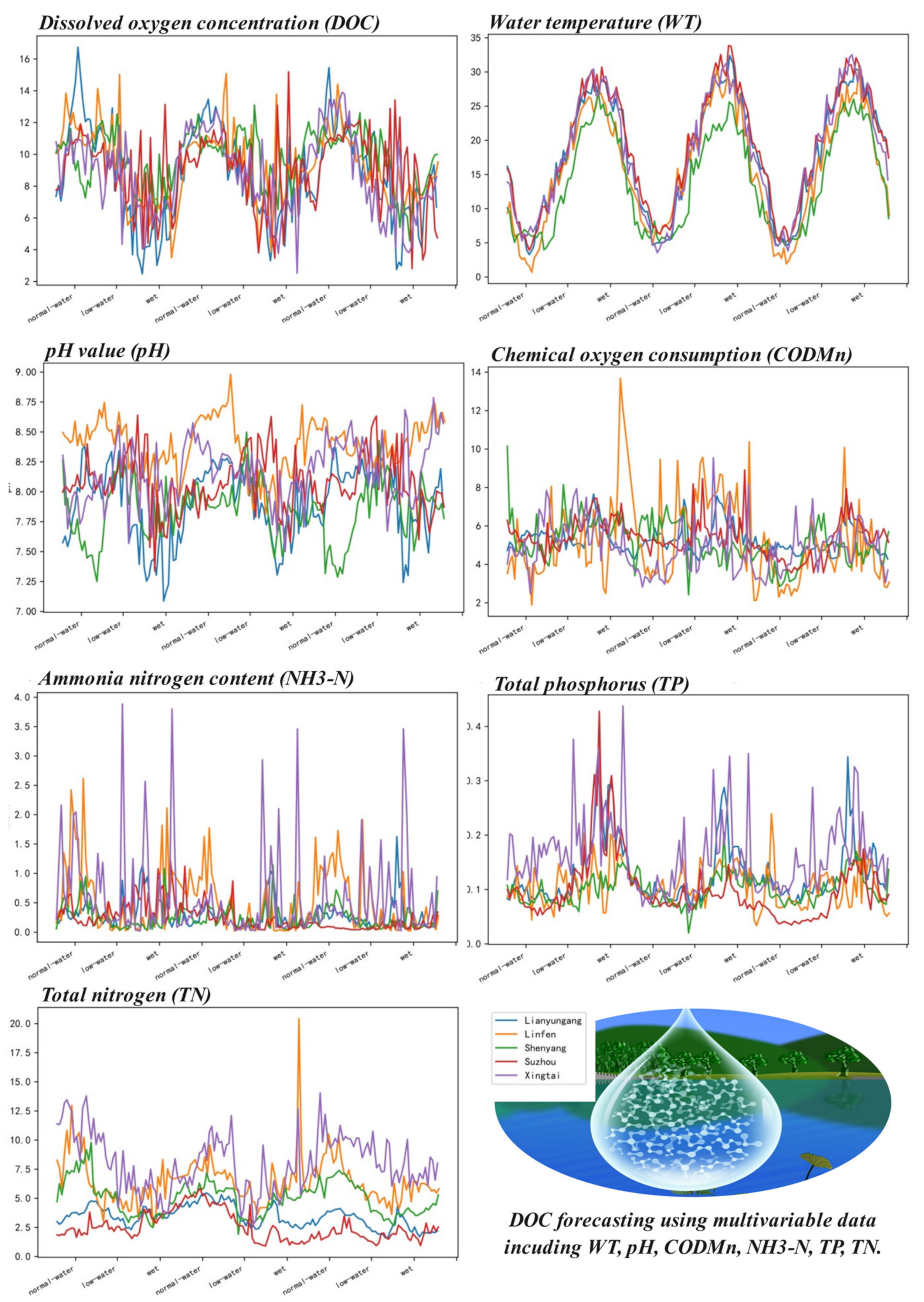
The DOCs of the five cities and their descriptive statistics are shown in

Table 1. Details of five DOC datasets from China.

Dataset	Sampling Frequency	Range	Variables	Samples	Numbers	DOC Statistical Indicators
						Mean	Std.	Min	Max
Lianyungang	4 h each time	8 November 2020–11 November 2023	DOC, pH, NH3-N, TN, WT, CODMn, TP	All	6588	8.8004	3.0982	1.9346	17.2613
				Training	5270	9.3010	3.0887	2.1907	17.2614
				Validating	659	7.1038	2.5465	1.9346	13.6383
				Testing	659	6.4962	1.7340	2.3959	11.1893
Shenyang	4 h each time	8 November 2020–11 November 2023	DOC, pH, NH3-N, TN, WT, CODMn, TP	All	6588	9.7186	1.9910	3.6453	15.5095
				Training	5270	9.9893	1.8700	3.6453	15.5095
				Validating	659	8.9858	2.1984	4.1184	14.7788
				Testing	659	8.2874	1.9168	3.9901	12.6585
Xintai	4 h each time	8 November 2020–11 November 2023	DOC, pH, NH3-N, TN, WT, CODMn, TP	All	6588	8.8607	2.6916	0.3800	20.1115
				Training	5270	9.3898	2.5796	0.3800	20.1115
				Validating	659	7.1153	1.9362	2.1620	15.8850
				Testing	659	6.3755	2.0019	0.9830	10.9100
Linfen	4 h each time	8 November 2020–11 November 2023	DOC, pH, NH3-N, TN, WT, CODMn, TP	All	6588	9.6140	2.6219	1.7110	28.9044
				Training	5270	10.0000	2.7142	1.7110	28.9044
				Validating	659	8.5213	1.5497	4.1295	16.5814
				Testing	659	7.6200	1.0254	5.3739	10.3716
Suzhou	4 h each time	8 November 2020–11 November 2023	DOC, pH, NH3-N, TN, WT, CODMn, TP	All	6588	8.9217	2.4038	2.2186	18.3548
				Training	5270	9.0951	2.2255	2.5726	18.3548
				Validating	659	8.8640	2.7437	2.2504	17.7152
				Testing	659	7.5937	2.9401	2.2186	15.1440

Note: Water quality dataset from China.

. As can be seen from Figure 2, the DOC started to decline after reaching the highest value during the normal water period; then, it started to decline continuously and reached the lowest value during the low-water season; however, it rebounded after the wet season. Concerning pH, the values did not fluctuate significantly during the normal water period but began to decline during the low-water season and gradually rebounded after the onset of the wet season. Regarding NH3-N, the values were higher and fluctuated more significantly towards the end of the wet season and at the beginning of the normal water period and were lower around the low-water season. For TN, its value continued to decrease from the normal water period to the low-water season, decreasing to the minimum value in the low-water season before rising continuously from the wet season to the normal water period. The WT value showed obvious periodicity, according to the normal water period, low-water period, and wet period, showing a “low-high-low” trend. The CODMn value changed more smoothly during each water period. The TP value changed stably in the normal water period but exhibited notably higher values and significant fluctuations at the end of the low-water season and the beginning of the wet season. In general, the numerical values of the seven water quality evaluation indicators showed obvious periodicity. DOC, pH, NH3-N, and TN reached their highest values in the normal water period and their lowest values in the low-water season. The trends relating to WT, CODMn, and TP exhibit inverse patterns, with annual peak and trough concentrations observed during the low-water and wet seasons.

Figure 2 shows that the changes in DOC are in line with physical and chemical laws, with low temperatures during the normal water period reducing the amount of oxygen dissolved within aquatic environments. On the contrary, during the low-water season, the rise in water temperature can lead to a decrease in both water level and water body fluidity, which is detrimental to the supply of dissolved oxygen. Suitable temperatures during the low-water season favor the growth and reproduction of microorganisms, which can utilize ammonia nitrogen (NH3-N) and total nitrogen (TN) for metabolic activities, leading to lower concentrations of both NH3-N and TN. CODMn and TP reach their peak values during the low-water season. Water flow is usually low during the low-water season, which may cause pollutants in the water body to be less easily washed away. Anoxic conditions or low oxygen in the water may also reduce the presence of manganese in the bottom sediments, releasing it into the water to form permanganate. Slowing plant growth activity also reduces total phosphorus uptake. This shows that there are deeper connections between the seven water quality evaluation indicators used, including WT, pH, CODMn, NH3-H, TP, TN, and DOC. Thus, the integration of the remaining six water quality indicators is essential for predicting the concentration of a single indicator: DOC.

3. Methodology

3.1. Convolutional Neural Network

Convolutional neural networks (CNNs) can effectively extract local feature patterns from input data, including images and sequence data [36]. CNNs are characterized by the hierarchical extraction of low-level to high-level features. Their advantages include superior performance, parameter sharing, sparse connectivity to reduce computational burden, automatic feature learning, and the ability to adapt to different tasks. Nonlinear activation functions, such as ReLU, follow the convolutional layer to introduce a nonlinear transformation, aiding the model in learning complex features effectively. Subsequently, the pooling layer downsamples the feature map, reducing its size while preserving essential information. Following the extraction of features, a fully connected layer is typically utilized to associate these features with their respective output categories. In the CNN architecture, the convolutional layer serves as the central component, tasked with utilizing the convolutional kernel $C_j$ to extract intrinsic features.

$$C_j=\sigma \left(\sum A_i\otimes {\omega }_i+b_i\right)$$

(3)

where $A_i$ denotes the input, ⊗ denotes the input, $\sigma$ denotes the activation function, ${\omega }_i$ denotes the weight associated with the kernel corresponding to the $i$-th feature map, and $b_i$ symbolizes the bias matrix.

3.2. Gated Recurrent Unit

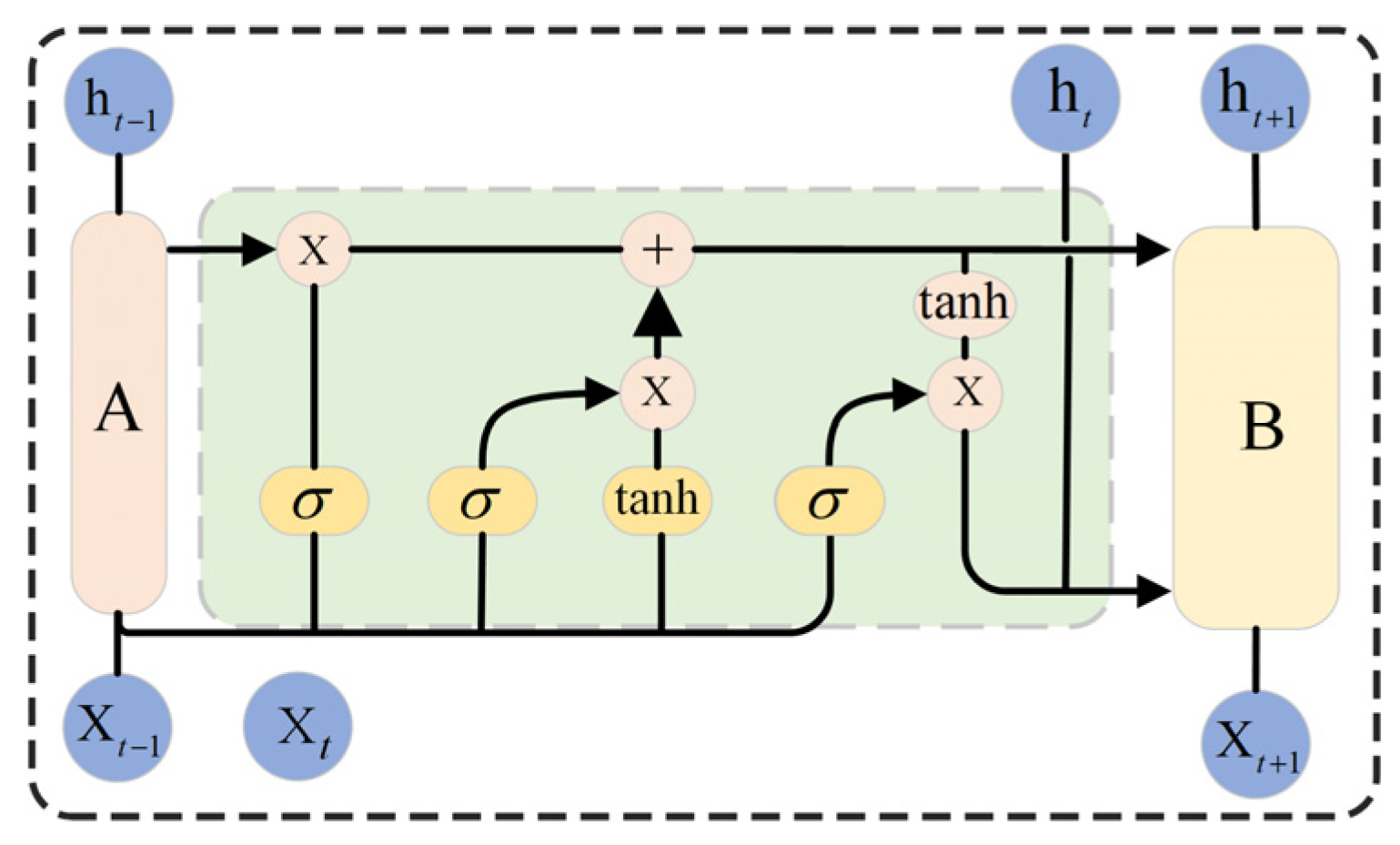
A Gated Recurrent Unit (GRU) represents a variant of a recurrent neural network specifically designed to handle sequential data [37]. A GRU can retain and update important information in sequence data through a gating mechanism, which can effectively capture the dynamic features of sequences and help alleviate the common problem of gradient vanishing when training recurrent neural networks. A GRU features a simpler architecture with fewer gating mechanisms and fewer parameters, which helps to effectively prevent overfitting when the volume of data is small. A GRU effectively captures long-range dependencies in sequence data by dynamically adjusting the reset and update gates. Moreover, a GRU may outperform LSTM on some short-sequence tasks. This is because the simplified structure of a GRU makes it easier and faster to train, meaning that it is suitable for resource-limited environments. In a GRU, the functionality of the forgetting gate and input gate in LSTM is consolidated into a single update gate. An elevated value of the update gate signifies the greater integration of state information from the preceding time step. Additionally, a smaller reset gate implies less influence from the previous state. A diagram of a GRU module is shown in Figure 3.

The calculations for each unit in the GRU module are shown below:

$$r_t=\sigma \left(W_{xr}{x}_t+W_{hr}{h}_{t-1}+b_r\right)$$

(4)

$$z_t=\sigma \left(W_{xz}{x}_t+W_{hz}{h}_{t-1}+b_z\right)$$

(5)

$$h_t^{\prime }=\mathit{tan}h\left[W_{xh}{x}_t+W_{hh}\left(r_t\odot h_{t-1}\right)+b_h\right]$$

(6)

$$h_t=\left(1-z_t\right)\odot h_{t-1}+z_t\odot h_t^{\prime }$$

(7)

where $x_t$ represents the input at moment $t$. $r_t$ denotes the reset gate. $z_t$ denotes the update gate. $h_t$ is the output hidden state at moment $t$.${ h}_t^{\prime }$ signifies the candidate hidden state at time $t$. $W$ and $b$ denote the corresponding weight parameters and bias parameters. The gate employs the sigmoid activation function denoted by $\sigma$. The hyperbolic tangent activation function tanh characterizes its functionality. The meaning of $\odot$ is the matrix point multiplication number means the matrix dot product number.

3.3. Attention Mechanism

Attention mechanism (AM) functions are vital when handling sequential data in deep learning [38], allowing a model to pay more attention to information in different locations when processing input sequences, thus improving a model’s ability to model long-distance dependencies. Incorporating an attention layer into a neural network aims to prioritize significant information by assigning higher weights while downplaying less relevant information with lower weights. These weights are dynamically adjusted throughout the training process, enhancing the network’s scalability and resilience over time.

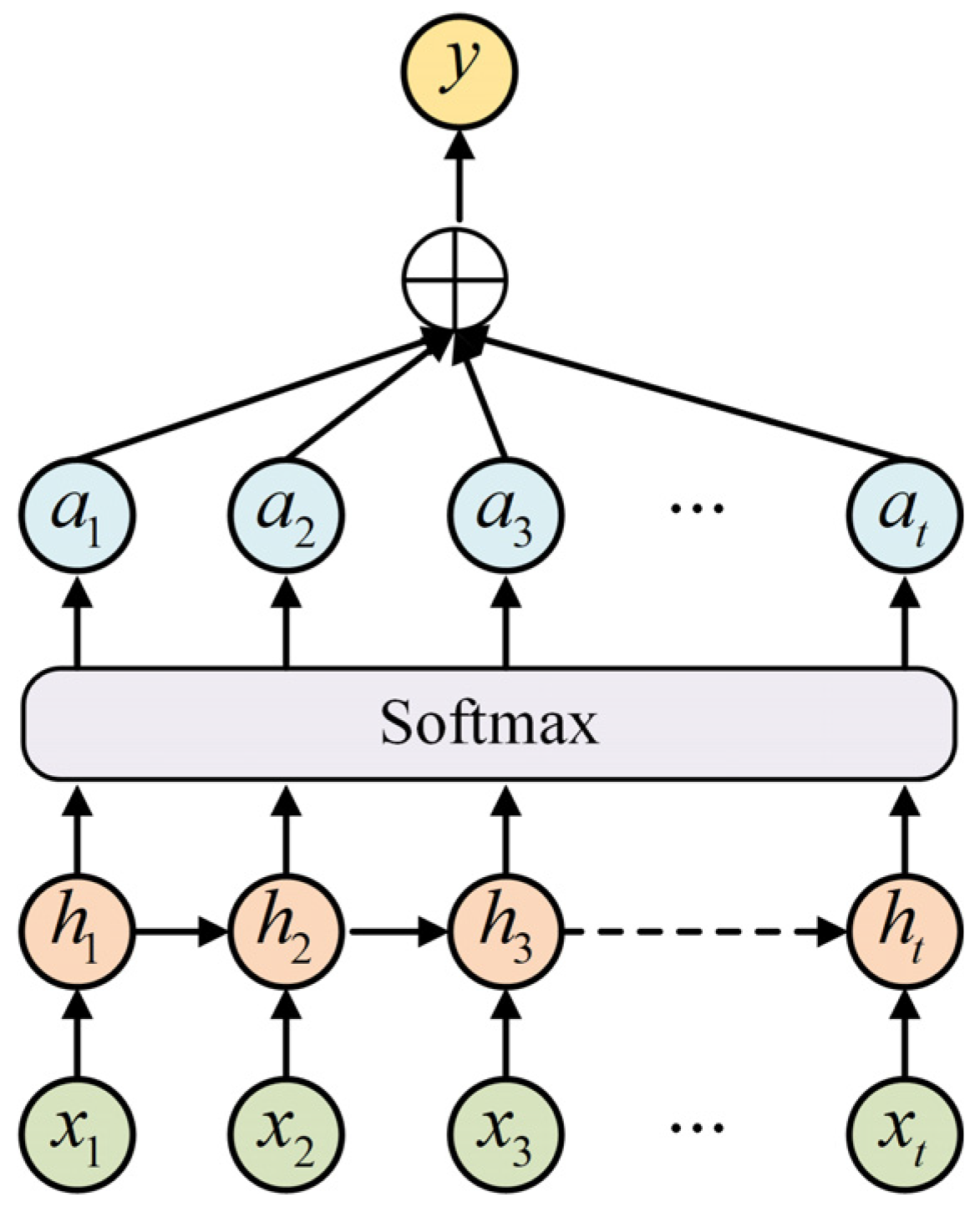
The input of the water quality is a time series fed into a GRU as a vector $x_1,x_2,\dots ,x_t$. The resulting GRU layer outputs the vector $h_1,h_2,\dots ,h_t$. Following the integration of the attention layer, individual input vectors exhibit varying degrees of impact on the model’s predicted outcome, as depicted in Figure 4. Consequently, assigning a probability distribution value to each vector ${\mathsf{\alpha }}_1,{\alpha }_2,\dots ,{ \alpha }_{t }$ becomes imperative, yielding the attention weight matrix and the corresponding feature representation V, as outlined in Equation (8):

$$V={\sum }_{t=1}^t{\alpha }_t{h}_t$$

(8)

3.4. Variational Mode Decomposition

Variational Mode Decomposition (VMD) stands out as an entirely intrinsic, adaptable, and non-recursive approach that can be used for signal decomposition [39]. It operates by solving a constrained variational problem, transforming the signal into K bandwidth-limited intrinsic mode functions (IMFs) within the frequency domain. This method can avoid the estimation errors caused by empirical modal decomposition (EMD) and local mean decomposition (LMD), representing the envelope estimation error in decomposition due to the recursive decomposition mode. It has powerful nonlinear and nonsmooth signal processing capabilities and has significant advantages in terms of solving problems concerning signal noise and avoiding modal aliasing compared to signal decomposition methods such as EMD and ensemble empirical modal decomposition (EEMD). However, the number of IMF submodalities K of VMD significantly influences the decomposition results. If K is too small, the decomposed sequence will lose too much information, leading to mode aliasing. If K is too large, the problem of over-decomposition will occur. The VMD process is as follows:

Firstly, establish a constrained variational model.

$$\left\{\begin{array}{c}{}_{\left\{u_k\right\},\left\{w_k\right\}}{}^{min}\left\{{\displaystyle \sum _{k=1}^K}{\left|\right|{\partial }_t\left[\right(\delta \left(t\right)+{\displaystyle \frac{j}{\pi t}})\ast u_k(t\left)\right]e^{-jwkt}\left|\right|}_2^2\right\}\\ s.t.{\displaystyle \sum _{k=1}^K}{u}_k\left(t\right)=f\end{array}\right.$$

(9)

where $u_k\left(t\right)$ represents the IMF component. f denotes the original signal. k represents the total count of iterations. K represents the total count of decomposition modes.$\delta \left(t\right)$ denotes the shock function. $w_k$ indicates the center frequency of each component.

Secondly, by integrating the Lagrange multiplier $\lambda \left(t\right)$ and the quadratic penalty factor α, the constrained variational issue is transformed into an unconstrained format, simplifying the process of deriving the Lagrange formula, as shown in Equation (10):

$$\begin{gathered} L\left(\right\{u_k\},\{w_k\},\{\lambda \left\}\right)= \\ \mathsf{\alpha }\sum _{k=1}^K{||{\partial }_t[(\delta (t)+{\displaystyle \frac{j}{\pi t}})\ast u_k(t)]e^{-jwkt}||}_2^2 \\ +{||f(t)-\sum _{k=1}^K{u}_k(t)||}_2^2+〈\lambda (t),f(t)-\sum _{k=1}^K{u}_k(t)〉 \end{gathered}$$

(10)

where < > means the inner product.

The factor of penalty $\alpha$ and the amount of decomposition modes K are determined. The initial values of $u_k,w_k,\lambda$ are set and the order n = 0 is set. Then, cycle update $u_k$ and $w_k$ from 1 until k = K:

$${\widehat{u}}_k^{n+1}={\displaystyle \frac{\widehat{f}(w)-\sum _{i\ne k}{\widehat{u}}_i(w)+\frac{\widehat{\lambda }(w)}{2}}{1+2\alpha {(w-wk)}^2}}$$

(11)

$$w_k^{n+1}={\displaystyle \frac{{\int }_0^{\infty }w{\left|{\widehat{u}}_k\right(w\left)\right|}^{2}dw}{{\int }_0^{\infty }{\left|{\widehat{u}}_k\right(w\left)\right|}^{2}dw}}$$

(12)

Update the Lagrange operator further:

$${\widehat{\lambda }}^{n+1}(w)={\widehat{\lambda }}^n(w)+\tau (\widehat{f}(w)-\sum _{k=1}^K{\widehat{u}}_k^{n+1}(w))$$

(13)

Determine whether the convergence conditions are met:

$$\sum _{k=1}^K{\displaystyle \frac{{\left|\right|{\widehat{u}}_k^{n+1}-{\widehat{u}}_k^n\left|\right|}_2^2}{{\left|\right|{\widehat{u}}_k^n\left|\right|}_2^2}}<\epsilon$$

(14)

If satisfied, output K IMFs; otherwise, n = n + 1 continues.

3.5. Beluga Whale Optimization

The Beluga Whale Optimizer (BWO) [40] serves as a tool for tackling optimization challenges. This study set predictive indicator MSE as an optimization objective of the BWO algorithm to search the hyperparameters of the proposed system. Emulating beluga behavior such as swimming, foraging, and whale fall, the BWO integrates adaptive balance factors and whale fall probabilities that are crucial for regulating exploration and exploitation capabilities. Moreover, the incorporation of the Levy flight function bolsters the convergence on a global scale. The BWO treats beluga whales as agents for exploration by utilizing a population-based approach. The search agent location matrix is modeled as presented in Equation (15):

$${\rm X}=\left[\begin{array}{cccc}{{\rm X}}_{\mathrm{1,1}}& {{\rm X}}_{\mathrm{1,2}}& \dots & {{\rm X}}_{1,d}\\ {{\rm X}}_{\mathrm{2,1}}& {{\rm X}}_{\mathrm{2,2}}& \dots & {{\rm X}}_{2,d}\\ ⋮& ⋮& ⋮& ⋮\\ {{\rm X}}_{n,1}& {{\rm X}}_{n,2}& \dots & {{\rm X}}_{n,d}\end{array}\right]$$

(15)

For all belugas, their fitness values are stored accordingly, with $n$ representing size and $d$ indicating dimensionality:

$$F_{{\rm X}}=\left[\begin{array}{c}f\left(x_{\mathrm{1,1}},x_{\mathrm{1,2}},\dots ,x_{1,d}\right)\\ f\left(x_{\mathrm{2,1}},x_{\mathrm{2,2}},\dots ,x_{2,d}\right)\\ ⋮\\ f\left(x_{n,1},x_{n,2},\dots ,x_{n,d}\right)\end{array}\right]$$

(16)

Defined as the balancing factor $B_f$, the BWO algorithm can gradually shift from exploration to exploitation:

$$B_f=B_0\left(1-{\displaystyle \frac{T}{2T_{max}}}\right)$$

(17)

where $T$ denotes the current iteration number. T_max represents the maximum iteration count. $B_0$ denotes a random value within the range (0, 1) updated at each step of the iteration process. Exploration prevails when the equilibrium factor $B_f$ exceeds 0.5, whereas exploitation dominates when $B_f$ falls below 0.5. With the iteration count $T$ rising, the range of $B_f$ gradually narrows from (0, 1) to (0, 0.5), signaling a substantial shift in the probabilities associated with the developmental and exploratory phases. Specifically, the likelihood of the developmental phase increases proportionally with the escalation of $T$.

(1)

Exploration stage

By considering the swimming behavior of beluga whales, the exploration phase of BWO is established. The position of the exploration agent is determined through paired swimming of the beluga, and the position is iteratively updated in the following manner:

$$\left\{\begin{array}{c}{X}_{i,j}^{T+1}=X_{i,p_j}^T+\left(X_{r,p_1}^T-X_{i,p_j}^T\right)\left(1+r_1\right)\sin \left(2\pi r_2\right), j=even\\ X_{i,j}^{T+1}=X_{i,p_j}^T+\left(X_{r,p_1}^T-X_{i,p_j}^T\right)\left(1+r_1\right)\cos \left(2\pi r_2\right), j=odd\end{array}\right.$$

(18)

where the current number of iterations is denoted as $T$. The new position $v_j$ of the $v$-th beluga is in the $j$-th dimension. A random integer $p_j$ is selected from the $d$-dimension, representing the position of the beluga in the $p_j$ dimension random numbers. $r_1$ and $r_2$ are selected from the range (0, 1). $\sin \left(2\pi r_2\right)$ and $\cos \left(2\pi r_2\right)$ determine the orientation of the mirrored beluga’s fins towards the water. The updated positions reflect the synchronized or mirrored behavior of the beluga while swimming or diving, depending on whether odd or even dimensions are chosen. In the exploration phase, the use of two random numbers, $r_1$ and $r_2$, enhances the randomness of the operator.

(2)

Development stage

The predatory behavior of beluga whales served as inspiration. Based on the proximity of nearby beluga whales, cooperation among them can occur during foraging and movement. Beluga whales engage in cooperative hunting, select the optimal prey, and assess alternative options by exchanging location information and evaluating potential candidates. The incorporation of the Levy flight strategy aimed to enhance the convergence rate during the BWO development phase. Supposing the utilization of the Levy flight strategy for prey capture, the mathematical model is formulated as presented in Equation (19).

$$X_i^{T+1}=r_3{X}_{best}^T-r_4{X}_i^T+C_1·L_F·\left(X_r^T-X_i^T\right)$$

(19)

$T$ denotes the current iteration number and represents the current position of the beluga. $r_3$ and $r_4$ are random numbers between (0, 1). The random jump intensity $C_1=2r_4\left(1-{\displaystyle \frac{T}{T_{max}}}\right)$ represents the strength of Levy flight. The Levy flight function $L_F$ is defined as follows:

$$L_F=0.05\times {\displaystyle \frac{u\times \sigma }{{\left|v\right|}^{1/\beta }}}$$

(20)

$$\sigma ={\left({\displaystyle \frac{r\left(1+\beta \right)\times \sin \left(\pi \beta /2\right)}{r\left(\left(1+\beta \right)/2\right)\times \beta \times 2^{\left(\beta -1\right)/2}}}\right)}^{1/\beta }$$

(21)

where the random numbers $u$ and $v$ follow a normal distribution. $\beta$ is the default constant, which is 1.5.

(3)

Whale Fall

To simulate the descent pattern in each successive cycle, a subjective hypothesis is adopted to determine the probability of a whale falling among the population of individuals, thus simulating minor fluctuations within the population. Assuming that some of these beluga whales either migrated or were targeted and plunged into the depths of the ocean, maintaining a constant population size requires adjusting the position of the beluga and the descent rate to ascertain the updated position. The following is the expression of the mathematical model presented in Equation (22):

$$X_i^{T+1}=r_5{X}_i^T-r_6{X}_r^T+r_7{X}_{step}$$

(22)

$r_5$, $r_6$, and $r_7$ are random numbers between (0, 1). $X_{step}$ is the step size of the whale falling, which is defined as presented in Equation (23):

$$X_{step}=\left(u_b-l_b\right)exp\left(-{\displaystyle \frac{c_{2}T}{T_{max}}}\right)$$

(23)

where the step factor $c_2$ is linked to both the likelihood of a decrease in whale numbers and their overall population. The symbols $u_b$ and $l_b$ are used to denote the variable’s upper and lower bounds, respectively. The model employs a linear function to calculate the chance of a whale’s decline, as represented in Equation (24).

$$W_f=0.1-{\displaystyle \frac{0.05T}{T_{max}}}$$

(24)

The likelihood of a whale’s decline diminishes from an initial rate of 0.1 to 0.05 by the conclusion of the iterations, indicating a reduction in the risk to the beluga as it approached the food source throughout the optimization procedure.

4. Model

4.1. The VMD-BWO-CNN-GRU-AM Model

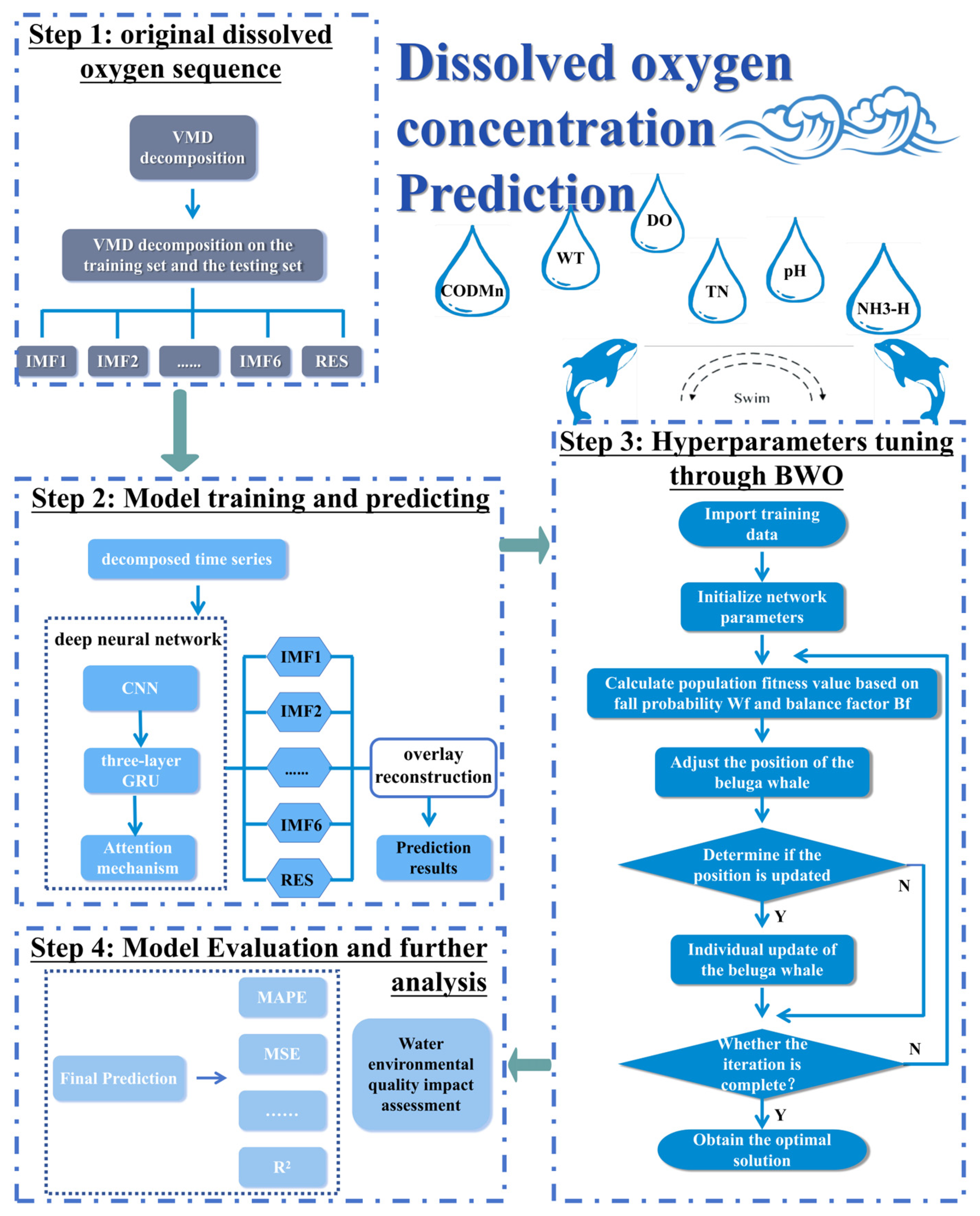
This study proposes a novel DOC prediction model that integrates VMD, CNN-GRU-AM, and BWO, as shown in Figure 5. Firstly, to improve prediction efficiency, the dataset is partitioned into training and testing subsets initially, and then the signal decomposition is carried out separately. The VMD algorithm decomposes data from the national automatic surface water quality monitoring system into a finite number of IMFs. Secondly, the CNN-GRU-AM is utilized to analyze the decomposed components obtained from VMD and other water quality indicators. Combining GRU, CNN, and AM can realize the ability of spatial local feature extraction and time series modeling for sequence data, thus improving training effectiveness and forecasting accuracy. Thirdly, the BWO algorithm is utilized to refine the hyperparameter setting of the proposed DOC forecasting system, which has efficiency and global optimization capabilities. The BWO mimics the reproductive and migratory behaviors of beluga whale groups, iteratively optimizing to find the optimal solution. Leveraging BWO enables the VMD-CNN-GRU-AM model to precisely and swiftly ascertain the optimal settings tailored to the attributes of water quality index data, thereby achieving efficient amalgamation.

The proposed DOC forecasting system consists of three parts: a VMD module to denoise the DOC sequence data, CNN-GRU-AM to extract complex features from the input data, and the BWO to determine the hyperparameters of the proposed DOC forecasting system. This study considers DOC datasets relating to five cities obtained from the urban areas with the worst water in China to verify the effectiveness of the proposed DOC forecasting system, providing a reference for water environment management. Each city includes 6588 data points in their four-hourly DOC datasets, including DOC, pH, NH3-N, TN, WT, CODMn, and TP. ${\mathit{D}\mathit{O}\mathit{C}}_{1th-5270th}$ are regarded as being training sets that can be used to train the proposed system. ${\mathit{D}\mathit{O}\mathit{C}}_{5271th-5929th}$ are regarded as being the validating sets that can be used to refine the parameters of the proposed system. ${\mathit{D}\mathit{O}\mathit{C}}_{5930th-6588th}$ are regarded as the test sets that can be used to estimate the effectiveness of the proposed system. $\mathit{D}\mathit{O}\mathit{C}$ can be understood as being the DOC dataset including DOC, pH, NH3-N, TN, WT, CODMn, and TP. $DOC$ is regarded as being the dissolved oxygen concentration sequence.

Step 1: Utilize VMD to decompose the original DOC sequence to denoise the original sequence, which can be written as ${\mathit{I}\mathit{M}\mathit{F}}_{1th-5270th}=f\left({DOC}_{1th-5270th}\right)$, ${\mathit{I}\mathit{M}\mathit{F}}_{5271th-5929th}=f\left({DOC}_{5271th-5929th}\right)$, and ${\mathit{I}\mathit{M}\mathit{F}}_{5930th-6588th}=f\left({DOC}_{5930th-6588th}\right)$. The K of the VMD is determined through experiments, which can effectively reduce sequence noise and improve predictability. All five cities adopt this operation.

Step 2: Operate CNN-GRU-AM to forecast IMF decomposed via VMD in Step 1, which can be written as ${IMF}_{t+w+1}^i=g\left({IMF}_{ttot+w}^i, {pH}_{ttot+w}, {NH3-NH}_{ttot+w}, {TN}_{ttot+w}, {WT}_{ttot+w}, {CODMn}_{ttot+w}, {TP}_{ttot+w}\right)$. In the training phase, 1 $\le t<$ 5270-w. In the validating phase, 5271 $\le t<$ 5929-w. In the testing phase, 5930 $\le t<$ 6588-w. w represents the rolling window size. $g\left(·\right)$ means the CNN-GRU-AM neural network. ${IMF}_{t+w+1}^i$ is the output of the neural network, which is the $t+w+1$ time point i-th IMF. ${IMF}_{ttot+w}^i, {pH}_{ttot+w}, {NH3-NH}_{ttot+w}, {TN}_{ttot+w}, {WT}_{ttot+w}, {CODMn}_{ttot+w}, {TP}_{ttot+w}$ is the input of the neural network, which includes the history i-IMF of the DOC and other water quality indicators. CNN-GRU-AM is utilized to extract the time patterns and the complex relationships between the water quality indicators. Then add the predicted IMF results, which can be written as ${DOC}_{t+w+1}=\sum _{i=1}^F{IMF}_{t+w+1}^i$. F represents the number of IMFs. We use the same K in the training set, validation set, and testing set to decompose, which avoids the modal misalignment or mismatch.

Step 3: Use the BWO to refine the hyperparameters of the proposed DOC forecasting system, which can obtain more accurate and robust DOC forecasting results. The BWO is used because the BWO results are better and it has greater computational efficiency. Use the ${\mathit{D}\mathit{O}\mathit{C}}_{5271th-5929th}$ dataset to refine the hyperparameter of the proposed DOC forecasting system. To search for the optimal parameter, this study considers the prediction accuracy mean square error (MSE) to be the optimization objective.

4.2. Model Evaluation

The statistical assessment metrics of mean absolute percentage error (MAPE), mean squared error (MSE), root mean squared error (RMSE), mean absolute error (MAE), and the coefficient of determination (R²) are used to measure the performance of the prediction model. These metrics can help objectively assess the accuracy and reliability of the model, thus providing confidence when interpreting the findings. MAPE measures the percentage of prediction errors. This method computes the absolute percentage error of the prediction for every observation, and then averages these figures. The lower the MAPE, the better the performance of the model. MSE is the mean of the squares of the prediction errors. It is more sensitive to large errors because the error is squared. A lower MSE value indicates the improved performance of the model. RMSE is the square root of MSE. It is similar to MSE but is identical in magnitude to the original target variable. As with MSE, smaller RMSE values indicate better model performance. MAE is the mean of the absolute values of the prediction errors. Unlike MAPE, MAE does not involve percentages and can be interpreted more easily. Smaller MAE values indicate better model performance. R² measures the model’s ability to explain changes in the target variable. It takes a value between 0 and 1, with results closer to 1 indicating a better explanation of the target variable by the model. When R² is 1, it indicates that the model fits the data perfectly.

4.3. Model Parameter Setting

The model parameter settings are presented in

Table 2. Parameter settings in proposed method.

Module	Parameters	Determination Method	Settings
Rolling window size	Window length	Experiment	42
CNN	Training optimization algorithms	Experiment	Adam
	Learning rate	Experiment	0.003
	Number of filters	Experiment	64
	Kernal Size	Experiment	5
	Activation function	Experiment	ReLU
GRU	First GRU Layer Neurons	Experiment	(BWO search)
	Second GRU Layer Neurons	Experiment	(BWO search)
	Third GRU Layer Neurons	Experiment	32
	Forth GRU Layer Neurons	Experiment	20
VMD	Number of Modes (K)	Experiment	8
	Alpha	Experience	2000
	Tolerance	Experiment	1 × 10−7
	Initial Center Frequencies	Experiment	1
	DC Component	Experiment	0
BWO	Population Size	Experiment	50
	Number of iterations	Experiment	50

.

5. Results

5.1. VMD Performance Evaluation

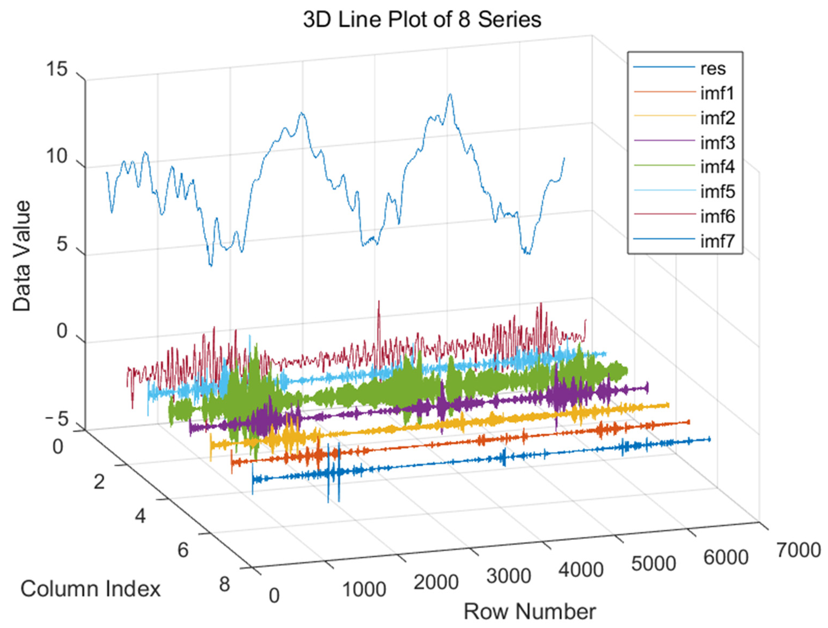
Figure 6 displays the VMD outcomes relating to the DOC in Lianyungang. The situation of other cities can be found in the online Supplementary Materials Figures S1–S4. The IMF unveils discernible patterns and cycles, capturing information across diverse temporal intervals within the original time series. As depicted in Figure 6, the x-axis indicates the sequential temporal frequency, while the y-axis signifies the temporal occurrence of each IMF and residual component (RES). Notably, in the high-frequency IMFs (IMF1, IMF1, and IMF3), significant fluctuations with slow oscillation rates characterize the IMF component, indicating marked instability in short-term dissolved oxygen concentrations. Transitioning to the intermediate frequency IMFs (IMF4 and IMF5), periodicity becomes evident with decreasing fluctuation frequency. Finally, in the low-frequency IMFs (IMF6 and IMF7), IMF component fluctuations level off, suggesting a plateauing trend in DOC data over time.

Table 3. Comparison of prediction accuracy between different decompositions.

City	Model	MSE	RMSE	MAE	R2	MAPE
Lianyungang	VMD-BWO-CNN-GRU-AM	0.0718	0.2680	0.2029	0.9922	0.0279
	EEMD-BWO-CNN-GRU-AM	0.1991	0.4462	0.3150	0.9794	0.0414
	CEEMDAN-BWO-CNN-GRU-AM	0.1440	0.3794	0.2800	0.9850	0.0386
Shenyang	VMD-BWO-CNN-GRU-AM	0.2573	0.5073	0.3487	0.9274	0.0365
	EEMD-BWO-CNN-GRU-AM	0.2634	0.5132	0.3510	0.9222	0.0370
	CEEMDAN-BWO-CNN-GRU-AM	0.2616	0.5114	0.3507	0.9223	0.0368
Linfen	VMD-BWO-CNN-GRU-AM	0.6984	0.8357	0.4806	0.8807	0.0524
	EEMD-BWO-CNN-GRU-AM	0.7979	0.8933	0.5172	0.8639	0.0556
	CEEMDAN-BWO-CNN-GRU-AM	0.7768	0.8813	0.5121	0.8670	0.0547
Suzhou	VMD-BWO-CNN-GRU-AM	0.1648	0.4060	0.2782	0.9687	0.0342
	EEMD-BWO-CNN-GRU-AM	0.1794	0.4236	0.3099	0.9611	0.0421
	CEEMDAN-BWO-CNN-GRU-AM	0.1717	0.4144	0.3168	0.9646	0.0392
Xingtai	VMD-BWO-CNN-GRU-AM	0.5298	0.7279	0.4647	0.9298	0.0603
	EEMD-BWO-CNN-GRU-AM	0.5528	0.7435	0.4866	0.9208	0.0627
	CEEMDAN-BWO-CNN-GRU-AM	0.5335	0.7304	0.4699	0.9273	0.0605

presents the predictive outcomes of VMD, EEMD, and CEEMDAN decomposition.

VMD-BWO-CNN-GRU-AM obtains better RMSE and MAPE, which are significantly lower than EEMD-BWO-CNN-GRU-AM and CEEMDAN-BWO-CNN-GRU-AM. Overall, VMD exhibits a more pronounced effect in terms of enhancing the prediction accuracy of the DOC model compared to EEMD and CEEMDAN.

5.2. BWO Performance Evaluation

This study employed the BWO to optimize neural numbers within the CNN-GRU-AM model. To underscore the efficacy of the BWO algorithm, we juxtaposed it with more commonplace optimization techniques such as Fish School Search (FSS) [41], Particle Swarm Optimization (PSO) [42], and the Whale Optimization Algorithm (WOA) [43] for comparative analysis. Finally, the prediction results of the model relating to the DOC datasets of five cities when using the BWO, FSS, PSO, and WOA algorithms are shown in

Table 4. Contrast in prediction accuracy among various optimization techniques.

City	Model	MSE	RMSE	MAE	R2	MAPE
Lianyungang	VMD-BWO-CNN-GRU-AM	0.0718	0.2680	0.2029	0.9922	0.0279
	VMD-FSS-CNN-GRU-AM	0.1484	0.3853	0.2876	0.9846	0.0387
	VMD-PSO-CNN-GRU-AM	0.1934	0.4398	0.3199	0.9799	0.0438
	VMD-WOA-CNN-GRU-AM	0.2005	0.4477	0.3242	0.9792	0.0412
Shenyang	VMD-BWO-CNN-GRU-AM	0.2573	0.5073	0.3487	0.9274	0.0365
	VMD-FSS-CNN-GRU-AM	0.2655	0.5153	0.3513	0.9220	0.0372
	VMD-PSO-CNN-GRU-AM	0.2710	0.5206	0.3531	0.9217	0.0377
	VMD-WOA-CNN-GRU-AM	0.2718	0.5213	0.3558	0.9214	0.0381
Linfen	VMD-BWO-CNN-GRU-AM	0.6984	0.8357	0.4806	0.8807	0.0524
	VMD-FSS-CNN-GRU-AM	0.7056	0.8400	0.4907	0.8794	0.0534
	VMD-PSO-CNN-GRU-AM	0.7161	0.8462	0.4959	0.8776	0.0537
	VMD-WOA-CNN-GRU-AM	0.7536	0.8681	0.4980	0.8712	0.0540
Suzhou	VMD-BWO-CNN-GRU-AM	0.1648	0.4060	0.2782	0.9687	0.0342
	VMD-FSS-CNN-GRU-AM	0.1684	0.4103	0.2784	0.9680	0.0344
	VMD-PSO-CNN-GRU-AM	0.1704	0.4127	0.2844	0.9677	0.0357
	VMD-WOA-CNN-GRU-AM	0.1708	0.4132	0.3117	0.9676	0.0381
Xingtai	VMD-BWO-CNN-GRU-AM	0.5298	0.7279	0.4647	0.9298	0.0603
	VMD-FSS-CNN-GRU-AM	0.5495	0.7413	0.4731	0.9272	0.0606
	VMD-PSO-CNN-GRU-AM	0.5520	0.7430	0.4851	0.9269	0.0626
	VMD-WOA-CNN-GRU-AM	0.6152	0.7843	0.4894	0.9185	0.0632

. Generally, compared with FSS, PSO, and WOA, BWO significantly enhances the prediction accuracy of the proposed model.

5.3. Model Comparisons

To showcase the efficacy of the proposed model, individual forecasts for DOC prediction outcomes were conducted for five cities. Subsequently, these models included SVM, LSTM, BP, TCN, GRU, CNN-GRU-AM, BWO-CNN-GRU-AM, and VMD-BWO-CNN-GRU-AM.

Table 5. Statistical assessment of various model performances regarding DOC.

City	Model	MSE	RMSE	MAE	R2	MAPE
Lianyungang (Site 1)	SVM	0.8517	0.9229	0.7812	0.8812	0.1183
	LSTM	0.5245	0.7071	0.5245	0.9471	0.0708
	BP	0.9444	0.9718	0.7350	0.9027	0.1006
	TCN	0.5347	0.7312	0.5686	0.9429	0.0700
	GRU	0.3577	0.5981	0.4568	0.9618	0.0685
	CNN-GRU	0.2691	0.5187	0.3646	0.9734	0.0485
	CNN-GRU-AM	0.2440	0.4940	0.3328	0.9757	0.0452
	BWO-CNN-GRU-AM	0.2149	0.4635	0.3166	0.9770	0.0423
	VMD-BWO-CNN-GRU-AM	0.0718	0.2680	0.2029	0.9922	0.0279
Shenyang (Site 2)	SVM	0.3428	0.5855	0.4790	0.5156	0.0728
	LSTM	0.5318	0.7282	0.5504	0.8643	0.0591
	BP	1.0983	1.0480	0.8346	0.7164	0.0906
	TCN	0.4371	0.6611	0.5031	0.8894	0.0519
	GRU	0.3504	0.5920	0.4312	0.9113	0.0444
	CNN-GRU	0.3186	0.5649	0.3974	0.9227	0.0426
	CNN-GRU-AM	0.2867	0.5354	0.3625	0.9304	0.0393
	BWO-CNN-GRU-AM	0.2729	0.5224	0.3617	0.9309	0.0384
	VMD-BWO-CNN-GRU-AM	0.2781	0.5273	0.3558	0.9274	0.0381
Linfen (Site 3)	SVM	3.1191	1.7660	1.5460	0.1471	0.3073
	LSTM	3.0075	1.7342	1.0137	0.5583	0.0989
	BP	3.7728	1.9424	1.2819	0.4522	0.1323
	TCN	2.3375	1.5289	0.8804	0.6598	0.0904
	GRU	2.0800	1.4422	0.8208	0.6973	0.0887
	CNN-GRU	1.5637	1.2505	0.7411	0.7717	0.0799
	CNN-GRU-AM	1.5497	1.2449	0.6727	0.7543	0.0730
	BWO-CNN-GRU-AM	1.4580	1.2074	0.6674	0.7602	0.0692
	VMD-BWO-CNN-GRU-AM	0.6984	0.8357	0.4806	0.8807	0.0524
Suzhou (Site 4)	SVM	1.3276	1.1522	0.8678	0.6386	0.1375
	LSTM	1.0578	1.0285	0.7218	0.8095	0.0961
	BP	2.2151	1.4883	1.1040	0.6053	0.1388
	TCN	0.7262	0.8521	0.5886	0.8692	0.0750
	GRU	0.6179	0.7861	0.5496	0.8887	0.0738
	CNN-GRU	0.6092	0.7805	0.5404	0.8976	0.0686
	CNN-GRU-AM	0.5578	0.7469	0.4935	0.9071	0.0645
	BWO-CNN-GRU-AM	0.5512	0.7223	0.4848	0.9053	0.0627
	VMD-BWO-CNN-GRU-AM	0.1648	0.4060	0.2782	0.9687	0.0342
Xingtai (Site 5)	SVM	2.4147	1.5539	1.2504	0.3432	0.2348
	LSTM	1.0649	1.0319	0.7198	0.8535	0.0963
	BP	2.0370	1.4272	0.9935	0.7267	0.1314
	TCN	0.8451	0.9193	0.6243	0.8837	0.0815
	GRU	0.7379	0.8590	0.5930	0.8985	0.0743
	CNN-GRU	0.7168	0.8466	0.5391	0.8994	0.0714
	CNN-GRU-AM	0.6579	0.8111	0.5129	0.9076	0.0665
	BWO-CNN-GRU-AM	0.6166	0.7852	0.4897	0.9152	0.0651
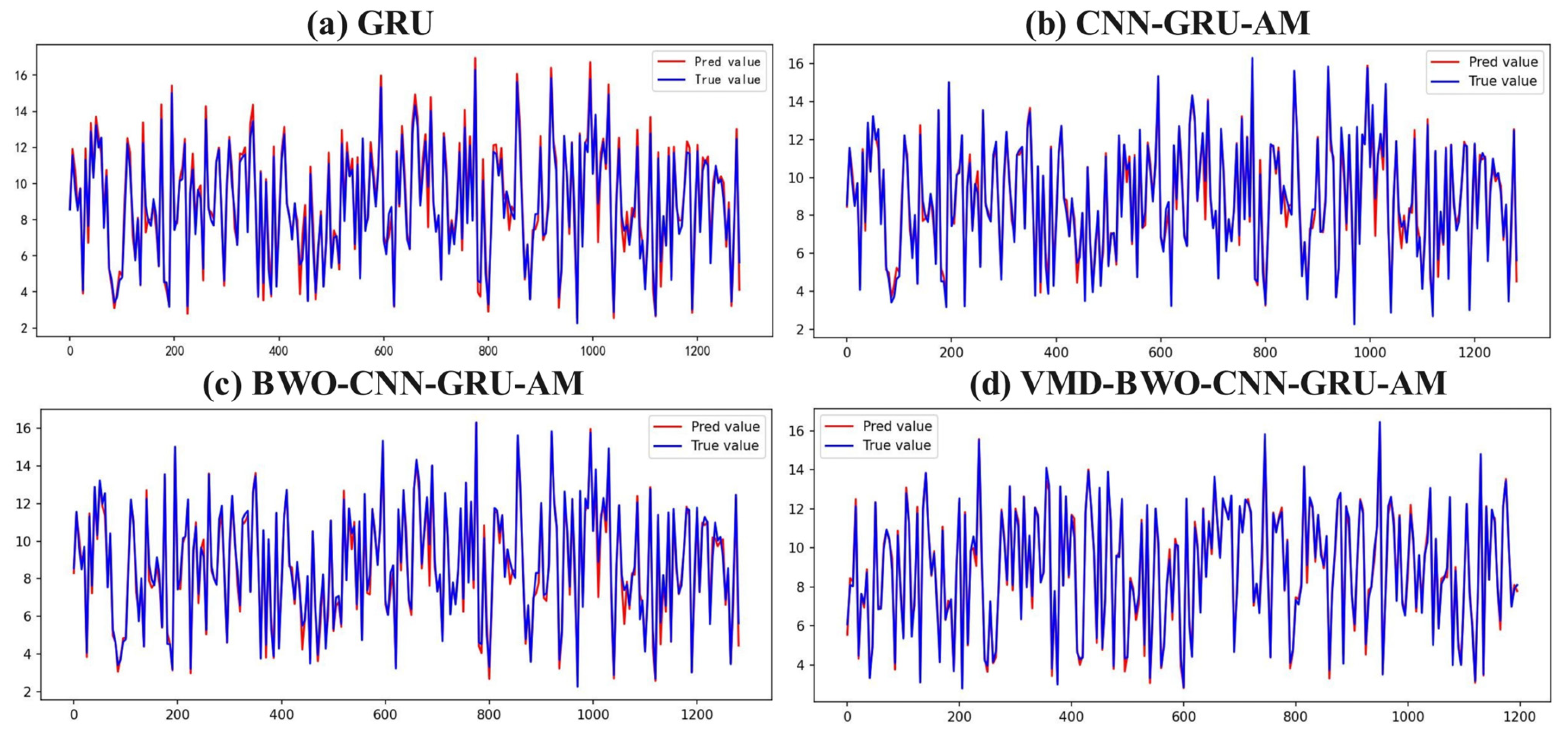
	VMD-BWO-CNN-GRU-AM	0.5520	0.7430	0.4851	0.9269	0.0636

presents the MSE, RMSE, MAE, R2, and MAPE values obtained from different models. Overall, the VMD-BWO-CNN-GRU-AM model demonstrates superior prediction accuracy, exhibiting the lowest MSE, RMSE, and MAE, along with the highest R², across the five cities. Moreover, as illustrated in Figure 7, the DOC prediction curve of this model when using the Lianyungang dataset closely corresponds with the observed curve, underscoring its high prediction precision. Hence, these findings underscore the proposed model’s validity, robustness, and superiority when compared to alternative approaches.

In particular, the predictive precision of the VMD-based model notably exceeds that of the non-based model, as evidenced by comparisons between the VMD-BWO-CNN-GRU-AM and BWO-CNN-GRU-AM models. Taking Lianyungang as an example, the predictive accuracy of the VMD-BWO-CNN-GRU-AM model increased by 1.52% in terms of R2, while the prediction error decreased by 14.31% in terms of MSE, 19.55% in terms of RMSE, 11.37% in terms of MAE, and 1.44% in terms of MAPE. This underscores the effectiveness of signal decomposition technology in mitigating the non-stationarity of DOC data and enhancing performance. Furthermore, the necessity of VMD is substantiated by the results presented in Table 4. It can be noted that the exclusion of VMD led to minimal enhancements in prediction accuracy when utilizing a CNN for feature screening and a GRU for extracting sequence patterns. Across the five selected cities, the R2 values demonstrated modest increases, ranging from approximately 0.89% to 7.44%, while MSE, RMSE, MAE, and MAPE exhibited decreases, varying from about 0.51% to 8.86%, 0.56% to 7.94%, 0.92% to 9.22%, and 0.18% to 2.00%, respectively. Consequently, the research concludes that incorporating VMD before utilizing a CNN for feature screening and GRU for extracting sequence patterns improved model accuracy and decreased errors.

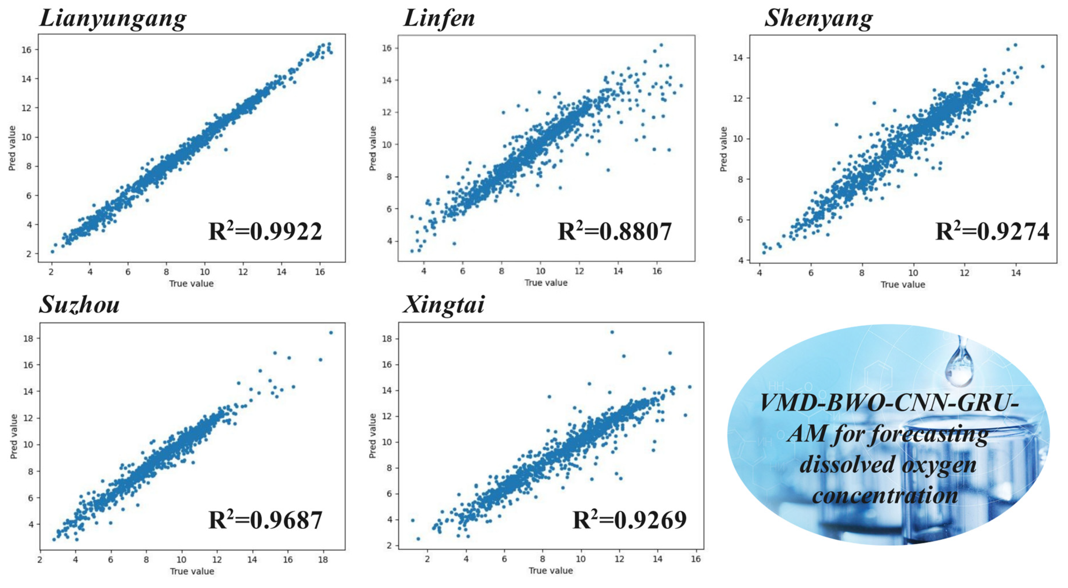
In general, the proposed model shows better predictive effects concerning DOCs. The predicted scatter plots shown in Figure 8 for different cities show that the proposed model has the highest R² value. The distribution of scattered points is uniform on either side of the diagonal line, with the fitted line being nearest to the diagonal line. The proposed DOC forecasting system, VMD-BWO-CNN-GRU-AM, showed fitting advantages when compared to the other models.

5.4. Contrast Analysis

In this study, Equations (25) and (26) were introduced and utilized to evaluate superiority. The results of $P_{MAE }$ > 0 or $P_{MAPE }$ > 0 indicate that the proposed DOC forecasting system is better than others. The larger the value, the more significant the performance increase. The equations are as follows:

$$P_{MAE}=({MAE}_2-{MAE}_1)/{MAE}_2\times 100\%$$

(25)

$$P_{MAPE}=({MAPE}_2-{MAPE}_1)/{MAPE}_2\times 100\%$$

(26)

The results are shown in

Table 6. Improvements of the proposed model compared to other models.

Model	PMAE (100%)						PMAPE (100%)
Site	Site 1	Site 2	Site 3	Site 4	Site 5	Average	Site 1	Site 2	Site 3	Site 4	Site 5	Average
SVM	4.97%	1.47%	6.49%	18.01%	23.72%	10.93%	3.15%	1.42%	5.97%	3.93%	9.56%	12.12%
LSTM	26.46%	23.48%	18.22%	25.23%	31.47%	24.97%	27.12%	25.82%	12.39%	26.91%	33.86%	24.67%
BP	49.26%	51.29%	43.11%	50.31%	49.00%	48.59%	50.33%	52.76%	39.61%	48.92%	48.86%	48.46%
TCN	31.62%	19.20%	3.60%	6.80%	18.84%	16.01%	25.14%	17.53%	4.44%	5.47%	17.55%	12.89%
GRU	54.37%	65.14%	52.84%	46.78%	59.48%	55.72%	60.18%	41.29%	74.00%	48.44%	71.38%	55.99%
SVM-AM	12.56%	19.68%	28.17%	31.64%	40.99%	26.61%	23.09%	31.10%	27.46%	28.64%	46.59%	29.42%
LSTM-AM	58.70%	78.46%	59.45%	64.21%	88.22%	69.81%	62.61%	35.62%	28.62%	57.30%	33.47%	72.03%
BP-AM	126.93%	23.67%	72.20%	47.33%	37.62%	61.55%	82.53%	24.21%	39.34%	29.14%	72.01%	48.47%
TCN-AM	2.78%	15.99%	27.24%	39.77%	34.15%	23.99%	5.70%	48.79%	19.21%	14.35%	30.10%	28.23%
GRU-AM	67.17%	132.63%	187.06%	124.73%	179.12%	138.14%	55.22%	83.12%	187.52%	146.67%	73.97%	152.34%
CNN-SVM	14.49%	40.97%	45.36%	28.91%	30.47%	32.04%	30.72%	67.67%	34.15%	13.19%	48.15%	35.55%
CNN-LSTM	13.16%	54.33%	38.15%	44.07%	35.11%	36.96%	37.40%	122.07%	87.69%	53.10%	34.27%	41.72%
CNN-BP	1.21%	67.54%	10.03%	21.01%	9.76%	21.91%	0.45%	69.82%	19.67%	35.10%	15.82%	26.05%
CNN-TCN	2.78%	14.05%	6.43%	3.78%	5.89%	6.59%	0.98%	19.63%	7.65%	3.98%	5.14%	7.35%
CNN-GRU	8.54%	3.54%	5.60%	9.76%	20.10%	9.51%	10.43%	5.10%	5.78%	9.08%	16.31%	9.70%
Proposed model	-	-	-	-	-	-	-	-	-	-	-	-

. In this study, the VMD-BWO-CNN-GRU-AM prediction method demonstrated its effectiveness and accuracy when modeling the uncertainty of a DOC prediction system. To this end, this paper introduces classical components. On average, the proposed method shows better performance on all five datasets. Therefore, the proposed VMD-BWO-CNN-GRU-AM method for predicting DOC has improved compared to the other classical models mentioned above. In addition, the empirical studies in this study show that the BWO algorithm is an effective technique in terms of providing an appropriate solution to parameter overshoot in a DOC prediction architecture.

6. Discussions

In order to improve DOC prediction accuracy and thereby provide a scientific basis for water environment management and pollution prevention, this study proposes a hybrid DOC prediction system that combines VMD, CNN, GRU, and BWO. The advantages and significance of the model in this study must be discussed.

(1)

This study proposes a hybrid model for predicting urban dissolved oxygen with high accuracy. This study uses urban water quality monitoring data gathered every 4 h from November 2020 to November 2023. The empirical results show that performance indicators such as MSE, RMSE, MAE, and MAPE in VMD-BWO-CNN-GRU-AM are significantly improved when compared to a single model. Taking the Site 1 dataset as an example, these indicators are reduced by 0.2859, 0.3301, 0.2539, and 0.0406, respectively.

(2)

The hybrid DOC prediction model can be extended to national surface water quality automatic monitoring stations in different river basins. This study utilized five urban water quality datasets with the worst water quality from different river basins. This method has universal applicability and can effectively improve DOC prediction accuracy in national water control stations, providing a better DOC prediction accuracy forecasting method for other regions to help with water management.

(3)

The proposed DOC hybrid forecasting system has good health and social benefits. It can serve as an early warning system of water quality deterioration, especially in cases of organic pollution and eutrophication. Developing accurate predictive models for the key water quality parameter of DOC can assess the effects of disturbances (anthropogenic, such as pollution, or climatic, such as climate change) on the suitability of aquatic habitats and, therefore, on the health of aquatic species.

7. Conclusions

As an important factor involved in maintaining the ecological balance of water and promoting biodiversity, DOC directly affects the health and survival state of all kinds of water organisms and has a profound impact on human survival and health. The water anoxia phenomenon is a major problem in the current global water environment; it results from the interaction of many complex factors. It is urgent to accurately simulate and predict DOCs. The analysis of existing forecasting models revealed several problems, including insufficient requirements for prediction accuracy and robustness, the instability of univariate prediction, and inefficiency. To address these challenges, a novel approach termed the VMD-BWO-CNN-GRU-AM model was proposed to forecast DOCs by using multivariable water quality indicators. Specifically, this study utilized VMD to decompose the original train and test DOC sequence, respectively, improving efficiency. CNN-GRU-AM was constructed to extract the complex patterns of water quality data, meaning that it is more flexible and effective. Then, the BWO was employed to optimize the hyperparameters of the proposed system with the aim of improving forecasting accuracy.

Water quality datasets from five cities in China were employed to assess the effectiveness of the proposed DOC forecasting system. This DOC forecasting hybrid model exhibits the highest level of accuracy when compared to other models. Employing Lianyungang as an example, the hybrid model yielded the following performance metrics: an MSE of 0.0718, an RMSE of 0.2680, an MAE of 0.2029, an MAPE of 0.9922, and a R2 of 0.0279. Moreover, it can be concluded that the hybrid model can maintain the highest prediction accuracy in different cities.

Future research endeavors may entail in-depth examinations of additional variables such as wind speed, wind direction, aquatic metabolism, and other potential influencing factors. By incorporating these variables, the hybrid model can be further optimized, thereby enhancing its efficacy and overall performance. Information leakage in the hybrid model should be considered comprehensively, which can result in overestimating prediction accuracy. Additionally, incorporating spatiotemporal prediction models into DOC forecasting systems is necessary, which can enhance the accuracy and the universality of these models for many other regions.

References

1. Ding, F.; Zhang, W.; Cao, S.; Hao, S.; Chen, L.; Xie, X.; Li, W.; Jiang, M. Optimization of water quality index models using machine learning approaches. Water Res. 2023, 243, 120337. [Google Scholar] [CrossRef]
2. Wu, J.; Yu, X. Numerical investigation of dissolved oxygen transportation through a coupled SWE and Streeter-Phelps model. Math. Probl. Eng. 2021, 2021, 6663696. [Google Scholar] [CrossRef]
3. Du, B.; Huang, S.; Guo, J.; Tang, H.; Wang, L.; Zhou, S. Interval forecasting for urban water demand using PSO optimized KDE distribution and LSTM neural networks. Appl. Soft Comput. 2022, 122, 108875. [Google Scholar] [CrossRef]
4. Guo, J.; Sun, H.; Du, B. Multivariable time series forecasting for urban water demand based on temporal convolutional network combining random forest feature selection and discrete wavelet transform. Water Resour. Manag. 2022, 36, 3385–3400. [Google Scholar] [CrossRef]
5. Wang, J.; Qian, Y.; Zhang, L.; Wang, K.; Zhang, H. A novel wind power forecasting system integrating time series refining, nonlinear multi-objective optimized deep learning and linear error correction. Energy Convers. Manag. 2024, 299, 117818. [Google Scholar] [CrossRef]
6. Stajkowski, S.; Zeynoddin, M.; Farghaly, H.; Gharabaghi, B.; Bonakdari, H. A methodology for forecasting dissolved oxygen in urban streams. Water 2020, 12, 2568. [Google Scholar] [CrossRef]
7. Liu, H.; Yang, R.; Duan, Z.; Wu, H. A hybrid neural network model for marine dissolved oxygen concentrations time-series forecasting based on multi-factor analysis and a multi-model ensemble. Engineering 2021, 7, 1751–1765. [Google Scholar] [CrossRef]
8. Li, J.; Chen, J.; Chen, Z.; Nie, Y.; Xu, A. Short-term wind power forecasting based on multi-scale receptive field-mixer and conditional mixture copula. Appl. Soft Comput. 2024, 164, 112007. [Google Scholar] [CrossRef]
9. Nie, Y.; Li, P.; Wang, J.; Zhang, L. A novel multivariate electrical price bi-forecasting system based on deep learning, a multi-input multi-output structure and an operator combination mechanism. Appl. Energy 2024, 366, 123233. [Google Scholar] [CrossRef]
10. Faezeh, M.G.; Taher, R.; Mohammad, K.Z. Decision tree models in predicting water quality parameters of dissolved oxygen and phosphorus in lake water. Sustain. Water Resour. Manag. 2022, 9, 1. [Google Scholar]
11. Alnahit, O.A.; Mishra, A.K.; Khan, A.A. Stream water quality prediction using boosted regression tree and random forest models. Stoch. Environ. Res. Risk Assess. 2022, 36, 2661–2680. [Google Scholar] [CrossRef]
12. Lu, H.; Ma, X. Hybrid decision tree-based machine learning models for short-term water quality prediction. Chemosphere 2020, 249, 126169. [Google Scholar] [CrossRef]
13. Li, W.; Wu, H.; Zhu, N.; Jiang, Y.; Tan, J.; Guo, Y. Prediction of dissolved oxygen in a fishery pond based on gated recurrent unit (GRU). Inf. Process. Agric. 2020, 8, 185–193. [Google Scholar] [CrossRef]
14. Wang, X.; Tang, X.; Zhu, M.; Liu, Z.; Wang, G. Predicting abrupt depletion of dissolved oxygen in Chaohu lake using CNN-BiLSTM with improved attention mechanism. Water Res. 2024, 261, 122027. [Google Scholar] [CrossRef]
15. Liu, Y.; Zhang, Q.; Song, L.; Chen, Y. Attention-based recurrent neural networks for accurate short-term and long-term dissolved oxygen prediction. Comput. Electron. Agric. 2019, 165, 104964. [Google Scholar] [CrossRef]
16. Peng, L.; Wu, H.; Gao, M.; Yi, H.; Xiong, Q.; Yang, L.; Cheng, S. TLT: Recurrent fine-tuning transfer learning for water quality long-term prediction. Water Res. 2022, 225, 119171. [Google Scholar] [CrossRef]
17. Wu, X.; Chen, M.; Zhu, T.; Chen, D.; Xiong, J. Pre-training enhanced spatio-temporal graph neural network for predicting influent water quality and flow rate of wastewater treatment plant: Improvement of forecast accuracy and analysis of related factors. Sci. Total Environ. 2024, 951, 175411. [Google Scholar] [CrossRef]
18. Irwan, D.; Ali, M.; Ahmed, A.N.; Jacky, G.; Nurhakim, A.; Ping Han, M.C.; AlDahoul, N.; El-Shafie, A. Predicting water quality with artificial intelligence: A review of methods and applications. Arch. Comput. Methods Eng. 2023, 30, 4633–4652. [Google Scholar] [CrossRef]
19. Balahaha Fadi, Z.S.; Latif, S.D.; Ahmed, A.N.; Chow, M.F.; Murti, M.A.; Suhendi, A.; Balahaha Hadi, Z.S.; Wong, J.K.; Birima, A.H.; El-Shafie, A. Machine learning algorithm as a sustainable tool for dissolved oxygen prediction: A case study of Feitsui Reservoir, Taiwan. Sci. Rep. 2022, 12, 3649. [Google Scholar]
20. Antanasijević, D.; Pocajt, V.; Perić-Grujić, A.; Ristić, M. Multilevel split of high-dimensional water quality data using artificial neural networks for the prediction of dissolved oxygen in the Danube River. Neural Comput. Appl. 2019, 32, 3957–3966. [Google Scholar] [CrossRef]
21. Najwa Mohd Rizal, N.; Hayder, G.; Mnzool, M.; Elnaim, B.M.; Mohammed, A.O.Y.; Khayyat, M.M. Comparison between Regression Models, Support Vector Machine (SVM), and Artificial Neural Network (ANN) in River Water Quality Prediction. Processes 2022, 10, 1652. [Google Scholar] [CrossRef]
22. Zhang, Y.; Fitch, P.; Thorburn, J.P. Predicting the Trend of Dissolved Oxygen Based on the kPCA-RNN Model. Water 2020, 12, 585. [Google Scholar] [CrossRef]
23. Wang, J.; Qian, Y.; Gao, Y.; Lv, M.; Zhou, Y. A combined prediction system for PM2.5 concentration integrating spatio-temporal correlation extracting, multi-objective optimization weighting and non-parametric estimation. Atmos. Pollut. Res. 2023, 14, 101880. [Google Scholar] [CrossRef]
24. Wang, B.; Jin, C.; Zhou, L.; Shen, D.; Jiang, Z. Water quality prediction of Xili Reservoir based on long short-term memory network. J. Yangtze River Acad. Sci. 2023, 40, 64–70. [Google Scholar]
25. Kim, J.; Yu, J.; Kang, C.; Ryang, G.; Wei, Y.; Wang, X. A novel hybrid water quality forecast model based on real-time data decomposition and error correction. Process Saf. Environ. Prot. 2022, 162, 553–565. [Google Scholar] [CrossRef]
26. Dong, Y.; Wang, J.; Niu, X.; Zeng, B. Combined water quality forecasting system based on multiobjective optimization and improved data decomposition integration strategy. J. Forecast. 2023, 42, 260–287. [Google Scholar] [CrossRef]
27. Wang, K.; Liu, Y.; Xing, Q.; Qian, Y.; Wang, J.; Lv, M. An integrated system to significant wave height prediction: Combining feature engineering, multi-criteria decision making, and hybrid kernel density estimation. Expert Syst. Appl. 2024, 241, 122351. [Google Scholar] [CrossRef]
28. Jiang, P.; Nie, Y.; Wang, J.; Huang, X. Multivariable short-term electricity price forecasting using artificial intelligence and multi-input multi-output scheme. Energy Econ. 2023, 117, 106471. [Google Scholar] [CrossRef]
29. Heydari, S.; Nikoo, M.R.; Mohammadi, A.; Barzegar, R. Two-stage meta-ensembling machine learning model for enhanced water quality forecasting. J. Hydrol. 2024, 641, 131767. [Google Scholar] [CrossRef]
30. Wai, K.P.; Chia, M.Y.; Koo, C.H.; Huang, Y.F.; Chong, W.C. Applications of deep learning in water quality management: A state-of-the-art review. J. Hydrol. 2022, 613, 128332. [Google Scholar] [CrossRef]
31. Asiri, M.M.; Aldehim, G.; Alotaibi, F.A.; Alnfiai, M.M.; Assiri, M.; Mahmud, A. Short-term load forecasting in smart grids using hybrid deep learning. IEEE Access 2024, 12, 23504–23513. [Google Scholar] [CrossRef]
32. Hameed, M.M.; Razali, S.F.M.; Mohtar, W.H.M.W.; Rahman, N.A.; Yaseen, Z.M. Machine learning models development for accurate multi-months ahead drought forecasting: Case study of the Great Lakes, North America. PLoS ONE 2023, 18, e0290891. [Google Scholar] [CrossRef]
33. Na, M.; Liu, X.; Tong, Z.; Sudu, B.; Zhang, J.; Wang, R. Analysis of water quality influencing factors under multi-source data fusion based on PLS-SEM model: An example of East-Liao River in China. Sci. Total Environ. 2024, 907, 168126. [Google Scholar] [CrossRef]
34. Faraji, H.; Shahryari, A. Estimation of Water Quality Index and Factors Affecting Their Changes in Groundwater Resource and Nitrate and Fluoride Risk Assessment. Water Air Soil Pollut. 2023, 234, 608. [Google Scholar] [CrossRef]
35. Interlandi, J.S.; Crockett, S.C. Recent water quality trends in the Schuylkill River, Pennsylvania, USA: A preliminary assessment of the relative influences of climate, river discharge and suburban development. Water Res. 2003, 37, 1737–1748. [Google Scholar] [CrossRef]
36. Xu, S.; Li, W.; Zhu, Y.; Xu, A. A novel hybrid model for six main pollutant concentrations forecasting based on improved LSTM neural networks. Sci. Rep. 2022, 12, 14434. [Google Scholar] [CrossRef]
37. Chung, J.; Gulcehre, C.; Cho, K.H.; Bengio, Y. Empirical evaluation of gated recurrent neural networks on sequence modeling. arXiv 2014, arXiv:1412.3555. [Google Scholar]
38. Vaswani, A. Attention is all you need. Adv. Neural Inf. Process. Syst. 2017, 30, I. [Google Scholar]
39. Dragomiretskiy, K.; Zosso, D. Variational mode decomposition. IEEE Trans. Signal Process. 2013, 62, 531–544. [Google Scholar] [CrossRef]
40. Zhong, C.; Li, G.; Meng, Z. Beluga whale optimization: A novel nature-inspired metaheuristic algorithm. Knowl.-Based Syst. 2022, 251, 109215. [Google Scholar] [CrossRef]
41. Bastos Filho, C.J.A.; de Lima Neto, F.B.; Lins, A.J.C.C.; Nascimento, A.I.S.; Lima, M.P. A novel search algorithm based on fish school behavior. In Proceedings of the 2008 IEEE International Conference on Systems, Man and Cybernetics, Singapore, 12–15 October 2008; IEEE: Piscataway, NJ, USA, 2008; pp. 2646–2651. [Google Scholar]
42. Kennedy, J.; Eberhart, R. Particle swarm optimization. In Proceedings of the ICNN’95-International Conference on Neural Networks, Perth, WA, Australia, 27 November–1 December 1995; IEEE: Piscataway, NJ, USA, 1995; Volume 4, pp. 1942–1948. [Google Scholar]
43. Mirjalili, S.; Lewis, A. The whale optimization algorithm. Adv. Eng. Softw. 2016, 95, 51–67. [Google Scholar] [CrossRef]
Figure 1. Chinese River Basin Map.
Water 16 02966 g001
Figure 2. Variation of seven water quality evaluation indicators. Note: The specific water periods are divided into: normal water period (January–February and November–December), wet season (July–October), and low-water season (March–June).
Water 16 02966 g002
Figure 3. A module diagram of a standard GRU.
Water 16 02966 g003
Figure 4. Structure of the attention mechanism.
Water 16 02966 g004
Figure 5. Flow chart of dissolved oxygen concentration prediction based on the VMD-BWO-CNN-GRU model.
Water 16 02966 g005
Figure 6. Lianyungang’s DOC decomposition signals results.
Water 16 02966 g006
Figure 7. DOC prediction curves for four algorithms taking Lianyungang as an example.
Water 16 02966 g007
Figure 8. Scatter plot of actual and predicted DOC values derived from different cities (proposed model).
Water 16 02966 g008