Artificial Neural Networks (ANNs) and Multiple Linear Regression (MLR) Analysis Modelling for Predicting Chemical Dosages of a Water Treatment Plant (WTP) of Drinking Water

Abstract

As the quantity and quality of water resources decreases, the need for timely and valid prediction of the WTP of drinking water-used chemicals to produce quality drinking water for the final consumer increases. The question that arises is which prediction model performs better in predicting the chemical dosages used in a WTP of drinking water. ANNs or the MLR analysis models? The present study is a comparative study between the two aforementioned prediction models. The evaluation criteria chosen are: the Root Mean Square Error (RMSE), the Coefficient of Determination (R²), and the Pearson Correlation Coefficient (R). A previously optimised ensemble ANN model was chosen, which consisted of 100 neural networks, with 42 hidden nodes each, 10 inputs, and 4 outputs. On the other hand, four different scenarios in MLR analysis with dependent variables were examined: the ozone (O₃) concentration, the Anionic Polyelectrolyte (ANPE) dosage, the Poly-Aluminium Chloride hydroxide sulphate (PACl) dosage, and the chlorine (Cl_2(g)) dosage. As independent variables, 10 WTP operational and quality water variables were considered. According to RMSE results, the MLR model had better performance for the three (RMSE ANPE = 0.05 mg/L, RMSE PACl = 0.08 mg/L, and RMSE Cl_2(g) = 0.10 kg/h) of the four used WTP of drinking water chemicals, than the ANN model, which performed better for only one (RMSE O₃ = 0.02 mg/L). According to R² and R results, the ANN model had better performance compared to the MLR analysis model for all four variables. Based on the criterion of R² > 0.5, the ANN performance was satisfactory in predicting three variables: ANPE (R² = 0.772), PACl (R² = 0.742), and Cl_2(g) dosage (R² = 0.838, +23% and R = 0.91553, +11%). Respectively, the prediction of the MLR analysis model was evaluated as satisfactory only for the Cl_2(g) dosage (R² = 0.681, R = 0.82500). If someone wants to use the above described (ANN or MLR) scenarios to predict Cl_2(g) dosages, it is better to use the one with the smallest RMSE. If they are interested in fitting purposes, the one with the largest R², is preferable. Also, the ozone concentration variable showed low values of the R², in all cases, possibly due to the large variation in its values. This study further strengthens the opinion that ANNs are useful decision support tools for a WTP of a drinking water operator and can accurately and sufficiently mimic the decisions regarding the used chemical dosages, which is the main daily concern of the plant operator.

1. Introduction

This study is placed in the context of prediction models using either a part of modern Artificial Intelligence (AI), such as ANNs, or more classical statistical predicting methods, such as MLR analysis. This study intends to compare and evaluate the two aforementioned modelling and prediction approaches and intends to provide documented recommendations to WTPs of drinking water operators, concerning which of the two methods should be used, to save time and be as sure as possible of the result and validity of the prediction. The current state of the research field has been reviewed and it is assessed that corresponding comparisons and conclusions have been drawn from a number of other similar studies in the field of catchment hydrology, water quality, groundwater quality, coagulants dosages, lake dissolved oxygen, various species plant growth and missing rainfall data [1,2,3,4,5,6,7]. ANNs have been used for the prediction of many other environmental variables, including in the water sector, with satisfactory results, such as the prediction of free residual chlorine in water networks, Cr(VI) uptake, reaction cross-sections, Wastewater Treatment Plant (WWTP) effluent water quality [8,9,10,11], reconstruction of surface water temperature in lakes [12], Total Dissolved Solids (TDS) [13], Electrical Conductivity (EC) [14], and coagulant dosages [3,15,16,17,18]. Also, MLR analysis has been used, in a rapid and successful way, to predict surface water quality, flocculants dosages, bromate formation during ozonation, and the formation of disinfection by-products, trophic state of drinking water reservoirs, trihalomethane levels in tap water, and faecal coliform removal [3,6,19,20,21,22,23]. The ANN model evaluated in this study was previously optimised and takes into account the experience of a WTP operator, based on which the presence or absence of certain input variables was evaluated [15].

The premier aim and novelty of the current study is the comparison of two prediction methods (ANNs and MLR analysis), with the final goal of helping the WTP of drinking water operators to optimally select the chemical dosages, which are used on a daily basis and is the main daily concern of the operator [3,6,7,24].

2. Materials and Methods

2.1. Study Area

The Aposelemis WTP of drinking water is a conventional treatment plant of surface water located in the Municipality of Hersonissos, in the Prefecture of Heraklion, in the Region of Crete, Greece (Figure 1 and Figure 2). It includes the processes of ozonation, coagulation, flocculation, sedimentation, sand filtration, and, finally, chlorination. At the beginning of the water treatment processes, ozone gas (O₃), produced on site, is used as a pre-disinfectant and oxidizer agent. Pre-ozonation is followed by coagulation using Poly-Aluminium Chloride hydroxide sulphate (PACl) with the addition of Anionic Polyelectrolyte (AN PE), which is a water-soluble polymer that carries a negatively charged ion. Finally, the treated water is subjected to chlorination using chlorine gas (Cl_2(g)). The Aposelemis WTP maximum capacity is 110,600 m³/d, but it usually operates at 1/3 of its maximum capacity. It processes the surface water of the Aposelemis dam reservoir with physicochemical processes [15].

2.2. Data

The data used in this study were either collected from the Supervisory Control and Data Acquisition (SCADA) system or through measurements carried out in the treatment plant (TP) water quality control laboratory, according to standard methods [25] and accredited ISO methods. The data were collected daily, over a period of 38 months, which resulted in 1188 daily values for each of the 14 variables, which was, in total, 16,632 values for all variables used in the modelling process.

The data were normalised before being used in the modelling process. This was assessed as necessary, due to the different range of variables values [15]. After normalisation using the formula shown in Equation (1), the final variables values ranged between 0.0 and 1.0:

Normalised Data = (L − Min)/(Max − Min)

(1)

where L is the measured value, Max is the maximum value of measured value, and Min is the minimum value of measured value.

The statistics of used variables are shown in

Table 1. Statistics of used variables [15].

No	Variable	Unit	MIN	MAX	MEAN	STDEV
1	Daily difference in water reservoir height (ΔH)	m	−1.91 1	3.55	0.00	0.18
2	Daily supply of untreated water(Q)	m3/d	4271	71,858	39,062	9492
3	Turbidity of untreated water (T1)	NTU	0.07	562.00	6.61	22.12
4	pH of untreated water (pH1)		6.57	8.38	7.58	0.34
5	Turbidity of treated water (T2)	ΝΤU	0.01	0.74	0.16	0.08
6	pH of treated water (pH2)		6.42	8.03	7.30	0.32
7	Concentration of treated water chlorine (Cl2)	mg/L	0.02	0.90	0.44	0.11
8	Concentration of treated water Aluminium (Al)	μg/L	7.00	146.00	41.97	21.36
9	Daily consumption of TP electricity (El)	kWh	1060	19,788	9424	2892
10	O3 concentration (O3)	mg/L	0.00	0.20	0.05	0.02
11	Anionic polyelectrolyte dosage (ANPE)	mg/L	0.20	0.80	0.40	0.15
12	Poly- Aluminium Chloride hydroxide sulphate dosage (PACl)	mg/L	7.00	100.00	17.99	11.64
13	Chlorine dosage (Cl2(g))	kg/h	0.70	8.00	2.46	1.27
14	Water turbidity in the inlet of filtration beds (T3)	NTU	0.17	7.25	1.29	0.84

Note: ¹ A negative value in the variable ΔH means that the water level in the water reservoir had been decreased.

.

2.3. ANN and MLR Analysis Models Creation

Regarding the prediction of the Aposelemis WTP of drinking water chemicals dosages, an ANN model was constructed and optimised with a hyper-parameter optimisation method in a previous study (Figure 3) [16]. The optimised ANN consisted of 10 Inputs (ΔH, Q, T₁, pH₁, T₂, pH₂, Cl₂, Al, El, T₃), 42 hidden nodes, and 4 targets (O₃, ANPE, PACl, Cl_2(g)). The Neural Fitting Tool (nftool) of MATLAB R2019a was used for all the ANN generations and calculations. The Levenberg–Marquardt algorithm was used for ANN training, because of its rapid convergence, its minimal internal parameters, and for minimising errors in estimating the unknown node locations [2,10,15]. The 1188 available values per variable were divided randomly in three datasets (training, validation, and testing) for use in the ANNs. From the available data, 70% was used for training (832 individual values), 15% for validation (178 individual values), and 15% for testing (178 individual values) of the developed ANN models. The training dataset was used for training the ANN weights, the validation dataset was used during training for the early stopping of the algorithm to avoid overtraining and to ensure the generalisation capability of the model, and the testing was not used at all in either phase of training; therefore, it can provide us with an estimation of the model’s ability to predict unknown values, with which it was never trained.

On the other hand, four different MLR analysis scenarios were examined, with the stepwise variable selection method, using SPSS software (IBM SPSS Statistics, version 26). In each scenario, the dependent variable selected was, respectively, the dosage of ozone (O₃), ANPE, PACl, and chlorine (Cl_2(g)). In each of the four scenarios, the necessary conditions for the application of the MLR analysis were satisfied.

2.4. Model Evaluation

In this comparative study, the comparison between measured and predicted values of the constructed models was carried out using the most commonly used mathematical criteria: the Root Mean Square Error (RMSE), the Coefficient of Determination (R²) and, the Pearson Correlation Coefficient (R) [Equations (2)–(4)].

The Root Mean Square Error (RMSE) shows how much different, on average, the predictions are from the measured values, ranging from zero to positive infinity. Generally, a lower RMSE indicates a better model fit to the data. RMSE values equal to zero indicate a perfect fit with the actual measured values.

The Coefficient of Determination (R²), in a regression model, represents the proportion of the variance for a dependent variable, explained by the independent variable. Values of R² close to 1 indicate a very good model fit. According to literature reports, values of R² greater than 0.5 indicate a high correlation [11,15,16,19,26,27].

The Pearson Correlation Coefficient (R) shows the strength of the linear relationship between a dependent and a set of independent variables, with values close to 1 indicating a good model fit. In general, better performance of the model is achieved with lower RMSE (close to 0) and higher R and R² (close to 1) [3,6].

$$RMSE=\sqrt{{\displaystyle \frac{1}{n}}\sum _{i=1}^n{(y_{p_i}-y_i)}^2}$$

(2)

$$R^2=1-{\displaystyle \frac{\sum {{(y}_i-y_{p_i})}^2}{\sum {(y_i-\frac{\sum y_i}{n})}^2}}$$

(3)

$$R={\displaystyle \frac{\sum _{i=1}^n(y_{p_i}-\overline{y_{p_i}})(y_i-\overline{y_i)}}{\sum {(y_{p_i}-\overline{y_{p_i}})}^2\sqrt{\sum _{i=1}^n{(y_i-\overline{y_i})}^2}}}$$

(4)

where $y_{p_i}$ is the predicted value, $y_i$ is the measured value, $\overline{y_{p_i}}$ and $\overline{y_i}$ are the average predicted and measured values, and n is the number of observations.

3. Results

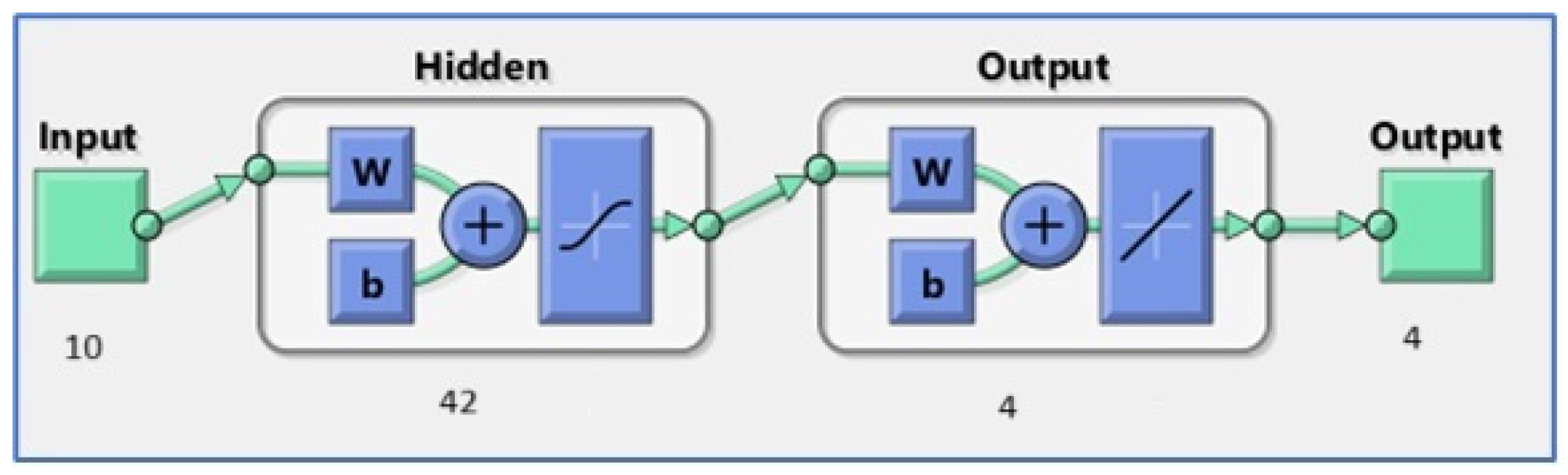
Regarding the ANN prediction, the scenario previously chosen (Figure 3) achieved very good simulation results based on best testing performance indicator (best tperf = 0.008848), which suggests that, in the drinking water sector, ANN modelling is a useful tool for the main operational variable prediction of a treatment plant of drinking water [15].

For each of the four ANN output parameters, the denormalisation equations [Equations (5)–(8)] of the parameters (where NV is the Normalised Value) are as follows [15]:

O₃ = 0.2 * NV_O3,

(5)

SP_ANPE = 0.2 + 0.6 * NV_SPANPE,

(6)

SP_PACl = 7 + 93 * NV_SPPACl,

(7)

SP_Cl2(g) = 0.7 + 7.30 * NV_SPCl2(g),

(8)

where SP is the Set Point.

Regarding the MLR analysis prediction,

Table 2. MLR Analysis R² values per studied scenario.

No	Dependent Variable	R2
1	O3	0.156
2	AN PE	0.236
3	PACl	0.501
4	Cl2(g)	0.681

shows the values of the multiple determination coefficient, R² (coefficient of determination), per scenario studied.

Among the studied scenarios, the best performing one is the one that had Cl_2(g) as a dependent variable. In that case, the value of R² = 0.681, which indicates a high correlation as mentioned above (R² > 0.5). The same criterion would suggest that the scenario having PACl as a dependent variable was also indicating borderline high correlation (R² = 0.501), but given the very high difference with the ANN results (R² = 0.742), this is not considered as a good alternative method. For the Cl_2(g) as a dependent variable, using the coefficients of Table 3, the equation of the MLR mathematical model is given by Equation (9). According to it, the prediction of gas chlorine dosage has a positive relationship with the WTP of drinking water daily electricity consumption, treated water turbidity, water supply, and untreated water turbidity, while it has a negative one with filtration bed inlet water turbidity, treated water residual Aluminium, and PACl dosage (normalised data).

Y = 0.070 + 0.511 * X₁ − 0.243 * X₂ + 0.362 * X₃ − 0.202 * X₄ − 0.319 * X₅ − 0.141 * X₆ + 0.130 * X₇ + 0.305 * X₈

(9)

Y: Chlorine dosage (kg/h)

Χ₁: Daily consumption of WTP electricity (kWh)

Χ₂: Water turbidity in the inlet of filtration beds (NTU)

Χ₃: Outlet water turbidity (NTU)

Χ₄: Outlet water residual Aluminium (μg/L)

Χ₅: Poly- Aluminium Chloride hydroxide sulphate (PACl) (ppm)

Χ₆: Outlet water pH

Χ₇: Water flow at the entrance of the WTP (m³/d)

Χ₈: Untreated water turbidity (NTU)

Table 3. MLR Analysis Coefficients ^a.

Step	Model	Unstandardized Coefficients		Standardised Coefficients	t	Sig.	Collinearity Statistics
		B	Std. Error	Beta			Tolerance	VIF
8	(Constant)	0.070	0.021		3.284	0.01	0.01
	Daily consumption of WTP electricity (kWh)	0.511	0.027	0.453	18.700	0.000	0.461	2.167
	Water turbidity in the inlet of filtration beds (NTU)	−0.243	0.032	−0.166	−7.690	0.000	0.581	1.721
	Turbidity of treated water (NTU)	0.362	0.031	0.222	11.802	0.000	0.763	1.311
	Concentration of treated water Aluminium (μg/L)	−0.202	0.022	−0.178	−9.064	0.000	0.699	1.430
	Polyaluminum sulphate chloride dosage (ppm)	−0.319	0.032	−0.229	−10.046	0.000	0.521	1.919
	pH of treated water	−0.141	0.021	−0.161	−6.864	0.000	0.495	2.021
	Daily supply of untreated water (m3/d)	0.130	0.025	0.105	5.127	0.000	0.650	1.537
	Turbidity of untreated water (NTU)	0.305	0.085	0.069	3.582	0.000	0.729	1.371

Note: ^a Dependent Variable: Chlorine gas flow (kg/h).

Table 3. MLR Analysis Coefficients ^a.

Step	Model	Unstandardized Coefficients		Standardised Coefficients	t	Sig.	Collinearity Statistics
		B	Std. Error	Beta			Tolerance	VIF
8	(Constant)	0.070	0.021		3.284	0.01	0.01
	Daily consumption of WTP electricity (kWh)	0.511	0.027	0.453	18.700	0.000	0.461	2.167
	Water turbidity in the inlet of filtration beds (NTU)	−0.243	0.032	−0.166	−7.690	0.000	0.581	1.721
	Turbidity of treated water (NTU)	0.362	0.031	0.222	11.802	0.000	0.763	1.311
	Concentration of treated water Aluminium (μg/L)	−0.202	0.022	−0.178	−9.064	0.000	0.699	1.430
	Polyaluminum sulphate chloride dosage (ppm)	−0.319	0.032	−0.229	−10.046	0.000	0.521	1.919
	pH of treated water	−0.141	0.021	−0.161	−6.864	0.000	0.495	2.021
	Daily supply of untreated water (m3/d)	0.130	0.025	0.105	5.127	0.000	0.650	1.537
	Turbidity of untreated water (NTU)	0.305	0.085	0.069	3.582	0.000	0.729	1.371

Note: ^a Dependent Variable: Chlorine gas flow (kg/h).

This model (Equation (9)) is statistically significant at a = 0.05 significance level (sig.= 0.000 < 0.05) as we can see from the ANOVA (

Table 4. MLR Analysis ANOVA table ^a.

Model	Sum of Squares	df	Mean Square	F	Sig.
Regression	25.541	8	3.068	314.350	0.000 i
Residual	11.505	1179	0.010
Total	36.047	1187

Note: ^a Dependent Variable: Chlorine gas flow (kg/h); ⁱ: Predictors: (Constant) daily consumption of WTP electricity (kWh), water turbidity in the inlet of filtration beds (NTU), turbidity of treated water (NTU), concentration of treated water Aluminium (μg/L), polyaluminium sulphate chloride dosage (ppm), pH of treated water, daily supply of untreated water (m³/d), turbidity of untreated water (NTU).

).

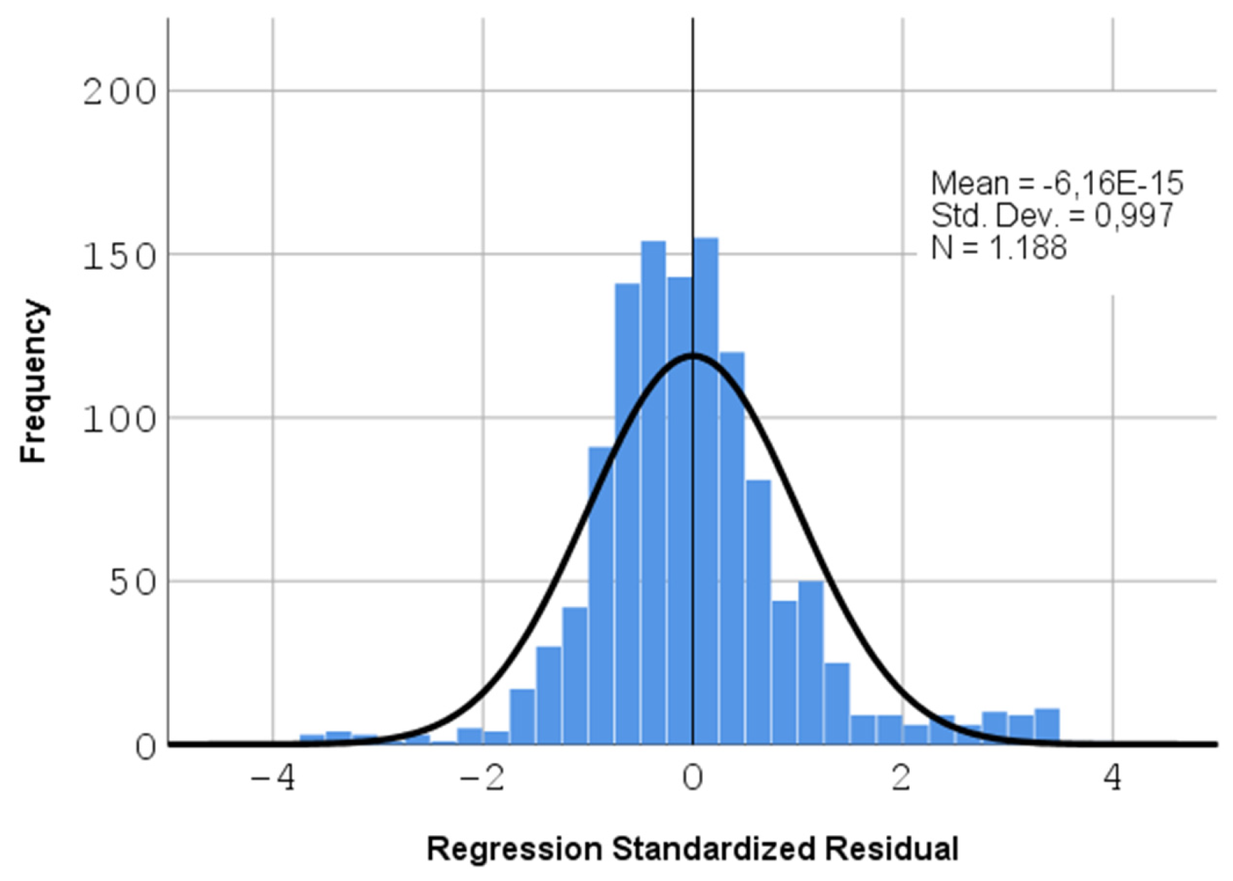
All the necessary conditions (e.g., normality, multi-collinearity, homoscedasticity, etc.) are being satisfied in this case. More precisely, the normality of the residuals of the model can be seen in the following histogram (Figure 4).

Multi-collinearity (i.e., the fact that the independent variables are (pairwise) being linearly related but not strongly is checked using the index Variance Inflation Factor (VIF), or Tolerance. Values of VIF more than 10 and Tolerance less than 0.20 show significant multi-collinearity between the variables. When significant multi-collinearity exists, it should be corrected, but from our analysis results, it is not the case here.

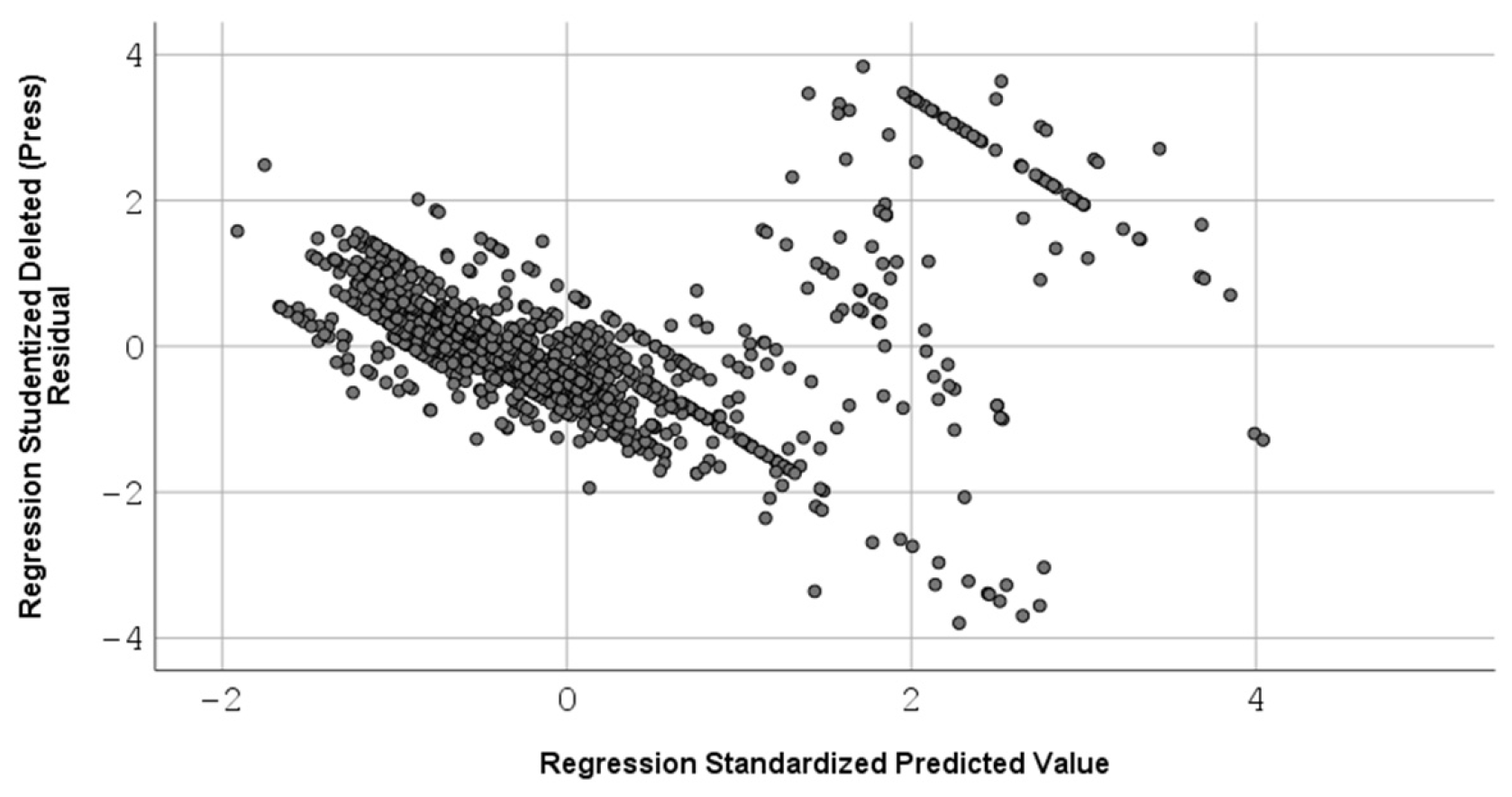
Homoscedasticity (the distribution of the dependent variable must remain the same for each combination of values of the independent variables): we notice the values of the Studentized deleted residuals (Figure 5), with a few exceptions, lie in the interval [−2, 2] and are almost uniformly (randomly) distributed over the entire range of predicted total values. So, the assumption of homoscedasticity or equality of variances is satisfied.

Regarding the required time for the two modelling approaches, it is worth mentioning that ANN development took a significant amount of time (≈389 min) until the final selection of the optimal network, while the MLR analysis required much less time (a few minutes), working on a laptop Intel Core i5 10th generation processor.

3.1. Root Mean Square Error (RMSE)

Table 5. RMSE values.

Variable	ANN	MLR
Residual O3 (mg/L)	0.02	0.09
ANPE dosage (mg/L)	0.07	0.05
PACl dosage (mg/L)	5.93	0.08
Cl2(g) dosage (Kg/h)	0.51	0.10

contains RMSE values for the ANN and MLR analysis prediction models per variable of interest. The physical unit of RMSE is different for each variable: mg/L for O₃, ANPE and PACl dosage, and kg/h for Cl_2(g) flow rate. The parameters R² and R are dimensionless quantities.

3.2. Coefficient of Determination (R²)

Table 6. R² values.

Variable	ANN	MLR	ANN vs. MLR
Residual O3	0.274	0.156
ANPE dosage	0.772	0.236
PACl dosage	0.742	0.501
Cl2(g) dosage	0.838	0.681	+23%

contains the R² values for the ANN and MLR analysis prediction models per variable of interest:

The MLR analysis, with the method of stepwise selection of variables (Stepwise method), using SPSS software, was carried out in eight different steps, and in the eighth step the value of R² was equal to 0.681, as shown in Table 2. So, the relationship between the dependent variable of Cl_2(g) dosage and the eight variables is strong and statistically significant (Sig. < 0.05).

3.3. Pearson Correlation Coefficient (R)

Table 7. R values.

Variable	ANN	MLR	ANN vs. MLR
Residual O3	0.52374	0.40100
ANPE dosage	0.87835	0.55200
PACl dosage	0.86157	0.73500
Cl2(g) dosage	0.91553	0.82500	+11%

contains R values for the ANN and MLR analysis prediction models per variable of interest:

4. Discussion

In this comparative study, two models were constructed by using ANNs and MLR analysis in MATLAB and SPSS, respectively, for WTP chemical dosages prediction. The data comes from a 38-month period of monitoring and recording (1188 daily values for each of the 14 variables, total: 16,632 values)

According to RMSE values of predicted and observed values of the ANN and MLR analysis prediction model (Table 5), the MLR model showed better performance for the three (RMSE ANPE = 0.05 mg/L, RMSE PACl = 0.08 mg/L and RMSE Cl_2(g) = 0.10 kg/h) of the four used WTP of drinking water chemicals, as compared to the ANN model, which was superior for only one of them (RMSE O₃ = 0.02 mg/L). Practically, the value of RMSE is the standard deviation of the prediction errors [11]. The value of this prediction, using the MLR model, is further enhanced if we consider that the average value of the ANPE dosage is 0.40 mg/L, the PACl dosage is 17.99 mg/L, and the Cl_2(g) dosage is 2.46 kg/h. Additionally, there are studies for the determination of WTP coagulant dosages in which MLR analysis modelling results performed slightly better (small RMSE and high R²) than ANN modelling [23]. According to bibliography in prediction modelling, the lower RMSE values and the higher the values of R² and R, the closer are the predicted values to the measured values [2,6].

Regarding the R² values, three of the four examined WTP of drinking water used chemical dosages that were (relatively) satisfactorily predicted by the selected ANN (Cl_2(g) dosage: R² = 0.838, ANPE dosage: R² = 0.772, PACl dosage: R² = 0.742 in descending order), while based on the MLR analysis, it was only one (Cl_2(g) dosage: R² = 0.681). The ozone concentration variable showed low values of the R², in all cases, possibly due to the large variation in its values. Based on the criterion of R² > 0.5, the prediction of the MLR analysis model was evaluated as satisfactory only for the Cl_2(g) dosage (R² = 0.681, R = 0.82500). Similar results have also been reported [1,3,6,7,28].

We must point out that if someone wants to use the above described (ANN or MLR) scenarios to predict Cl_2(g) dosages, it is better to use the one with the smallest RMSE. If they are interested in fitting purposes, it is better to use the one with the largest R².

According to WTP of drinking water operator experience, the fact that, according to MLR analysis, the prediction of Cl_2(g) dosage has a positive relationship with the daily electricity consumption, treated water turbidity, water flow, and raw water turbidity at the entrance of the WTP, can be explained by the increased burden on the quality of the untreated water, which leads to the increase in the consumption of electricity in the ozonation process and the turbidity of the finally treated water, due to the oxidation of the substances in the last stage of chlorination. In corresponding studies of predicting the WTP flocculants dosages, the designed MLR model presented that coagulant dosage had, respectively, a positive relationship with flow rate, temperature, and turbidity, while it had a negative relationship with pH and alkalinity [3,6].

According to Pearson Correlation Coefficient (R), a better prediction is achieved by the ANN model for the three of the four used chemicals (ANPE, PACl, Cl_2(g) dosage), while by the MLR analysis only for one (Cl_2(g)). The results of these metrics are shown for all variables in the respective tables (Table 6 and Table 7). The only variable that is clearly indicating a high correlation (R² > 0.5) is Cl_2(g) dosage. Compared to the R² and R values of the respective ANN results, the ANN outperforms the MLR analysis by 23% and 11%, respectively.

Similar studies of chemical dosages prediction in a WTP of drinking water have shown satisfactory results regarding the performance of the predictions and their high accuracy. Specifically, for chemical dosages predictions using ANNs, the values of the RMSE range from 0.64 to 5.93 mg/L and of R² from 0.742 to 0.940. The corresponding values for chemical dosages predictions using MLR analysis are as follows: RMSE ranges from 0.085 to 4.31 mg/L and R² ranges 0.63–0.9 [3,15,17,23,24,28].

In conclusion, the three used comparison metrics (RMSE, R², and R) show satisfactory results regarding the initial question: which prediction model performs better in predicting the dosages of chemicals used in a WTP of drinking water. The ANN models are much better than the corresponding MLR analysis prediction models, if we are mainly interested in the adaptability of the prediction, while if we are interested in having as few errors as possible in the predicted values, then MLR analysis seems to be better. Generally, ANN models can predict most of the chemicals used in a WTP. However, the prediction performance according to MRL is evaluated as satisfactory, for the case of Cl_2(g). This modelling study using ANNs and MLR analysis is considered very important as the performance of the predictions is satisfactory; the accuracy of the predictions is very high and in this way the prediction of a WTP of drinking water chemical dosages can be conducted by modelling and not by jar tests, which are time-consuming, expensive, and susceptible to human error. Additionally, the modelling results are immediately available, even during rapid and extreme changes in the quality characteristics of the raw water, saving money and human and water resources. Finally, this study further strengthens the opinion that ANN modelling is a useful decision support tool [15,29,30] for a WTP of drinking water operator and can accurate and sufficiently predict the decisions regarding the used chemical dosages that interests them every day.

Future studies are recommended to increase knowledge on the prediction of water chemicals used in a WTP of drinking water by using data-driven models, like ANNs, as an accurate prediction model and MLR analysis, as a flexible and fast but also reliable prediction model. Specifically, in the future, the estimation of the WTP of drinking water-used chemicals dosages, could be studied, using ANNs with only basic variables of the inlet water quality to build faster and more flexible ANN prediction models. Also, even more effort should be made to establish ANNs in the water sector and in the WTPs day-to-day operation [3,31,32]. Future research ideas include exploring the use of other comparison criteria, such as the Mean Absolute Error (MAE), the Mean Absolute Percentage Error (MAPE), or the Nash–Sutcliffe efficiency (NSE), as well as Principal Component Analysis to identify the most influencing parameters. A Sensitivity and Uncertainty Analyses focusing on the most influential parameters could further enhance the modelling process. Finally, given that the main limitation of the current work is that the models have been trained with data from a single WTP of drinking water, we suggest as future work, the inclusion of data for more WTPs of drinking water, in order to increase the robustness of the models and their universal applicability.

References

1. Alnuwaiser, M.A.; Javed, M.F.; Khan, M.I.; Ahmed, M.W.; Galal, A.M. Support Vector Regression and ANN Approach for Predicting the Ground Water Quality. J. Indian Chem. Soc. 2022, 99, 100538. [Google Scholar] [CrossRef]
2. Azeem, A.; Mai, W.; Tian, C.; Javed, Q. Dry Weight Prediction of Wedelia Trilobata and Wedelia Chinensis by Using Artificial Neural Network and MultipleLinear Regression Models. Water 2023, 15, 1896. [Google Scholar] [CrossRef]
3. Dadebo, D.; Obura, D.; Etyang, N.; Kimera, D. Economic and Social Perspectives of Implementing Artificial Intelligence in Drinking Water Treatment Systems for Predicting Coagulant Dosage: A Transition toward Sustainability. Groundw. Sustain. Dev. 2023, 23, 100987. [Google Scholar] [CrossRef]
4. Papailiou, I.; Spyropoulos, F.; Trichakis, I.; Karatzas, G.P. Artificial Neural Networks and Multiple Linear Regression for Filling in Missing Daily Rainfall Data. Water 2022, 14, 2892. [Google Scholar] [CrossRef]
5. Selim, A.; Shuvo, S.N.A.; Islam, M.M.; Moniruzzaman, M.; Shah, S.; Ohiduzzaman, M. Predictive Models for Dissolved Oxygen in an Urban Lake by Regression Analysis and Artificial Neural Network. Total Environ. Res. Themes 2023, 7, 100066. [Google Scholar] [CrossRef]
6. Lin, S.; Kim, J.; Hua, C.; Park, M.-H.; Kang, S. Coagulant Dosage Determination Using Deep Learning-Based Graph Attention Multivariate Time Series Forecasting Model. Water Res. 2023, 232, 119665. [Google Scholar] [CrossRef] [PubMed]
7. Li, L.; Rong, S.; Wang, R.; Yu, S. Recent Advances in Artificial Intelligence and Machine Learning for Nonlinear Relationship Analysis and Process Control in Drinking Water Treatment: A Review. Chem. Eng. J. 2021, 405, 126673. [Google Scholar] [CrossRef]
8. De Souza Batista, G.; Clemente De Lacerda, M.; Pires Aragão, D.; Cabral De Araújo, M.M.; Lima Rodrigues, A.C. Modeling the Decay of Free Residual Chlorine in Water Distribution Networks in Brazilian Rural Communities Using Artificial Neural Network. J. Water Process Eng. 2024, 61, 105312. [Google Scholar] [CrossRef]
9. Mu’azu, N.D. Insight into ANN and RSM Models’ Predictive Performance for Mechanistic Aspects of Cr(VI) Uptake by Layered Double Hydroxide Nanocomposites from Water. Water 2022, 14, 1644. [Google Scholar] [CrossRef]
10. Özdoğan, H.; Üncü, Y.A.; Şekerci, M.; Kaplan, A. Neural Network Predictions of (α, n) Reaction Cross Sections at 18.5±3 MeV Using the Levenberg-Marquardt Algorithm. Appl. Radiat. Isot. 2024, 204, 111115. [Google Scholar] [CrossRef]
11. Wongburi, P.; Park, J.K. Prediction of Wastewater Treatment Plant Effluent Water Quality Using Recurrent Neural Network (RNN) Models. Water 2023, 15, 3325. [Google Scholar] [CrossRef]
12. Sojka, M.; Ptak, M. Reconstruction of Surface Water Temperature in Lakes as a Source for Long-Term Analysis of Its Changes. Water 2024, 16, 3347. [Google Scholar] [CrossRef]
13. Farooq, M.U.; Zafar, A.M.; Raheem, W.; Jalees, M.I.; Aly Hassan, A. Assessment of Algorithm Performance on Predicting Total Dissolved Solids Using Artificial Neural Network and Multiple Linear Regression for the Groundwater Data. Water 2022, 14, 2002. [Google Scholar] [CrossRef]
14. Ekemen Keskin, T.; Özler, E.; Şander, E.; Düğenci, M.; Ahmed, M.Y. Prediction of Electrical Conductivity Using ANN and MLR: A Case Study from Turkey. Acta Geophys. 2020, 68, 811–820. [Google Scholar] [CrossRef]
15. Gyparakis, S.; Trichakis, I.; Diamadopoulos, E. Using Artificial Neural Networks to Predict Operational Parameters of a Drinking Water Treatment Plant (DWTP). Water 2024, 16, 2863. [Google Scholar] [CrossRef]
16. Baouab, M.H.; Cherif, S. Prediction of the Optimal Dose of Coagulant for Various Potable Water Treatment Processes through Artificial Neural Network. J. Hydroinform. 2018, 20, 1215–1226. [Google Scholar] [CrossRef]
17. Haghiri, S.; Daghighi, A.; Moharramzadeh, S. Optimum Coagulant Forecasting by Modeling Jar Test Experiments Using ANNs. Drink. Water Eng. Sci. 2018, 11, 1–8. [Google Scholar] [CrossRef]
18. Achite, M.; Farzin, S.; Elshaboury, N.; Valikhan Anaraki, M.; Amamra, M.; Toubal, A.K. Modeling the Optimal Dosage of Coagulants in Water Treatment Plants Using Various Machine Learning Models. Env. Dev. Sustain. 2022, 26, 3395–3421. [Google Scholar] [CrossRef]
19. Wang, A.; Wang, J.; Luan, B.; Wang, S.; Yang, D.; Wei, Z. Classification of Pollution Sources and Their Contributions to Surface Water Quality Using APCS-MLR and PMF Model in a Drinking Water Source Area in Southeastern China. Water 2024, 16, 1356. [Google Scholar] [CrossRef]
20. Zhang, J.; Ye, D.; Fu, Q.; Chen, M.; Lin, H.; Zhou, X.; Deng, W.; Xu, Z.; Sun, H.; Hong, H. The Combination of Multiple Linear Regression and Adaptive Neuro-Fuzzy Inference System Can Accurately Predict Trihalomethane Levels in Tap Water with Fewer Water Quality Parameters. Sci. Total Environ. 2023, 896, 165269. [Google Scholar] [CrossRef]
21. Osmane, A.; Zidan, K.; Benaddi, R.; Sbahi, S.; Ouazzani, N.; Belmouden, M.; Mandi, L. Assessment of the Effectiveness of a Full-Scale Trickling Filter for the Treatment of Municipal Sewage in an Arid Environment: Multiple Linear Regression Model Prediction of Fecal Coliform Removal. J. Water Process Eng. 2024, 64, 105684. [Google Scholar] [CrossRef]
22. Peng, F.; Lu, Y.; Wang, Y.; Yang, L.; Yang, Z.; Li, H. Predicting the Formation of Disinfection By-Products Using Multiple Linear and Machine Learning Regression. J. Environ. Chem. Eng. 2023, 11, 110612. [Google Scholar] [CrossRef]
23. Shi, Z.; Chow, C.W.K.; Fabris, R.; Liu, J.; Sawade, E.; Jin, B. Determination of Coagulant Dosages for Process Control Using Online UV-Vis Spectra of Raw Water. J. Water Process Eng. 2022, 45, 102526. [Google Scholar] [CrossRef]
24. Sharafi, M.; Rezaverdinejad, V.; Behmanesh, J.; Samadianfard, S. Development of Long Short-Term Memory along with Differential Optimization and Neural Networks for Coagulant Dosage Prediction in Water Treatment Plant. J. Water Process Eng. 2024, 65, 105784. [Google Scholar] [CrossRef]
25. Standard Methods for the Examination of Water and Wastewater, 23rd ed.; Bridgewater, L.L., Baird, R.B., Eaton, A.D., Rice, E.W., American Public Health Association, American Water Works Association, Water Environment Federation, Eds.; American Public Health Association: Washington, DC, USA, 2017; ISBN 978-0-87553-287-5. [Google Scholar]
26. Kim, C.M.; Parnichkun, M. MLP, ANFIS, and GRNN Based Real-Time Coagulant Dosage Determination and Accuracy Comparison Using Full-Scale Data of a Water Treatment Plant. J. Water Supply Res. Tec. 2017, 66, 49–61. [Google Scholar] [CrossRef]
27. Moriasi, D.N.; Arnold, J.G.; Van Liew, M.W.; Bingner, R.L.; Harmel, R.D.; Veith, T.L. Veith Model Evaluation Guidelines for Systematic Quantification of Accuracy in Watershed Simulations. Trans. ASABE 2007, 50, 885–900. [Google Scholar] [CrossRef]
28. Lin, S.; Kim, J.; Hua, C.; Kang, S.; Park, M.-H. Comparing Artificial and Deep Neural Network Models for Prediction of Coagulant Amount and Settled Water Turbidity: Lessons Learned from Big Data in Water Treatment Operations. J. Water Process Eng. 2023, 54, 103949. [Google Scholar] [CrossRef]
29. Lamrini, B.; Lakhal, E.K.; Le Lann, M.V. A Decision Support Tool for Technical Processes Optimization in Drinking Water Treatment. Desalination Water Treat. 2014, 52, 4079–4088. [Google Scholar] [CrossRef]
30. O’Reilly, G.; Bezuidenhout, C.C.; Bezuidenhout, J.J. Artificial Neural Networks: Applications in the Drinking Water Sector. Water Supply 2018, 18, 1869–1887. [Google Scholar] [CrossRef]
31. Doorn, N. Artificial Intelligence in the Water Domain: Opportunities for Responsible Use. Sci. Total Environ. 2021, 755, 142561. [Google Scholar] [CrossRef]
32. Xiang, X.; Li, Q.; Khan, S.; Khalaf, O.I. Urban Water Resource Management for Sustainable Environment Planning Using Artificial Intelligence Techniques. Environ. Impact Assess. Rev. 2021, 86, 106515. [Google Scholar] [CrossRef]
Figure 1. Aposelemis WTP of drinking water location.
Water 17 00227 g001
Figure 2. Aposelemis WTP of drinking water.
Water 17 00227 g002
Figure 3. ANN model structure.
Water 17 00227 g003
Figure 4. Histogram of Chlorine gas flow (kg/h) as a dependent variable.
Water 17 00227 g004
Figure 5. Regression Standardised predicted value of Cl2(g) flow (kg/h) vs. Regression Studentized Deleted Residual.
Water 17 00227 g005