Using Artificial Neural Networks to Predict Operational Parameters of a Drinking Water Treatment Plant (DWTP)

Abstract

The scope of the present study is the estimation of key operational parameters of a drinking water treatment plant (DWTP), particularly the dosages of treatment chemicals, using artificial neural networks (ANNs) based on measurable in situ data. The case study consists of the Aposelemis DWTP, where the plant operator had an estimation of the ANN output parameters for the required dosages of water treatment chemicals based on observed water quality and other operational parameters at the time. The estimated DWTP main operational parameters included residual ozone (O₃) and dosages of the chemicals used: anionic polyelectrolyte (ANPE), poly-aluminum chloride hydroxide sulfate (PACl), and chlorine gas (Cl_2(g)). Daily measurable results of water sample analysis and recordings from the DWTP Supervisory Control and Data Acquisition System (SCADA), covering a period of 38 months, were used as input parameters for the artificial neural network (1188 values for each of the 14 measurable parameters). These input parameters included: raw water supply (Q), raw water turbidity (T₁), treated water turbidity (T₂), treated water residual free chlorine (Cl₂), treated water concentration of residual aluminum (Al), filtration bed inlet water turbidity (T₃), daily difference in water height in reservoir (∆H), raw water pH (pH₁), treated water pH (pH₂), and daily consumption of DWTP electricity (El). Output/target parameters were: residual O₃ after ozonation (O₃), anionic polyelectrolyte (ANPE), poly-aluminum chloride hydroxide sulfate (PACl), and chlorine gas supply (Cl_2(g)). A total of 304 different ANN models were tested, based on the best test performance (tperf) indicator. The one with the optimum performance indicator was selected. The scenario finally chosen was the one with 100 neural networks, 100 nodes, 42 hidden nodes, 10 inputs, and 4 outputs. This ANN model achieved excellent simulation results based on the best testing performance indicator, which suggests that ANNs are potentially useful tools for the prediction of a DWTP’s main operational parameters. Further research could explore the prediction of water chemicals used in a DWTP by using ANNs with a smaller number of operational parameters to ensure greater flexibility, without prohibitively reducing the reliability of the prediction model. This could prove useful in cases with a much higher sample size, given the data-demanding nature of ANNs.

1. Introduction

Water treatment plant operators often seek a quick, easy-to-use, and reliable method to predict the daily dosages of chemicals. The present study focuses on meeting this need using ANNs to provide a useful and reliable tool for DWTP operators. This study uses historical data on the quality and operational parameters of a surface water treatment plant that produces water for human consumption (potable water). The importance of this study is that it takes into account the experience of the DWTP operator, a factor that has been largely absent from the existing literature.

Artificial intelligence is recognized as a powerful tool for solving many industrial operational problems and has been applied in various fields such as transportation, financial management, and healthcare [1,2,3]. Artificial intelligence has also found applications in the field of environmental monitoring, such as rainfall forecasting and water or wastewater treatment monitoring [3,4,5,6,7,8]. Recently, machine learning, a part of artificial intelligence, has also been employed in water resource management and treatment processes [9,10,11,12,13].

A reliable model for predicting the operating parameters of a water treatment plant is essential for controlling the operation of the plant and ensuring the provision of safe drinking water for consumers. Quality parameters such as turbidity, pH, and water temperature are often monitored, and there is a significant correlation between the aforementioned parameters and the quantities of flocculants and coagulants used in water treatment processes [11,14,15,16,17].

Artificial neural networks (ANNs), as a branch of artificial intelligence [18], are models designed to resemble the brain’s performance [18,19]. ANNs are very useful tools with high efficiency in complex relationship matching and forecasting in a DWTP setting. ANNs can process nonlinear data that are complex and difficult to simulate with simple mathematical models [12,15,17]. ANNs are based on learning, training, and control mechanisms and are not programmed like conventional computer programs. The training of an artificial neural network is achieved by adding the abovementioned connections through a training algorithm. Modelling using an artificial neural network is achieved based on the following main stages: 1. data collection, 2. data analysis, and 3. neural network training.

A neural network is capable of learning and therefore generalizing. These are the two main reasons that a neural network can make accurate predictions. Generalization is the production of logical output data for input data that is not encountered during the training of the artificial neural network. For this reason, an ANN is able to find appropriate simulation solutions to complex, data-rich, and otherwise intractable problems [19].

The most commonly used ANN types are: Multi-layer Perceptrons (MLPs), Radial Basis Function (RBF) networks, General Regression Neural Networks (GRNNs), Cascade Forward Networks (CFNs), and Kohonen’s self-organizing maps (SOM) [19,20,21,22]. Several studies have been published on the modelling and optimization of water treatment processes by using ANNs. Multilayer perceptron (MLP) artificial neural networks (ANNs) have been used for regression to determine flocculant dosages and turbidity of treated water [23,24]. Another approach, using machine vision, involved the use of a neural network to predict flocculant dosages by analyzing images of flocculation [25].

The values of the parameters of R² (coefficient of determination), MSE (Mean Squared Error), SSE (Sum of Squared Error), and RMSE (Root-Mean-Square Error) are commonly used for the validation of the results that are predicted from the models. Small deviations between model results and experimental results are usually observed [1,26].

According to previous research [1,15,17,27], the advantages of ANN modelling in the water sector include: (i) the lack of an algorithm required to build the ANN model, making modelling a fast and flexible process; (ii) the ability to handle nonlinear relationships with ease; (iii) the incorporation of the experience and knowledge of the plant operator into the construction of the model; (iv) the optimization of water treatment processes; (v) practical solutions to water pollution issues; (vi) reduction of operational expenditures by the optimization of chemical usage; and (vii) timely generation of modelling and forecasting results.

The limitations of ANN modelling in the water sector are: (i) the availability of data; (ii) poor data reproducibility; (iii) the need for sufficient data for training and testing; (iv) the dependence of the prediction performance of the model on specific conditions (e.g., great uncertainty in sudden changes); (v) disadvantages related to random data selection; and (vi) high computational requirements [1,18,28].

Building on previous studies that demonstrated the reliability of ANN-based prediction models in the field of surface water treatment, the purpose of this study was to predict the chemical dosages in a DWTP and assess whether ANNs could be useful tools for the operators of complex physicochemical water treatment processes, providing them with first estimates of chemical dosages.

2. Materials and Methods

2.1. Study Area

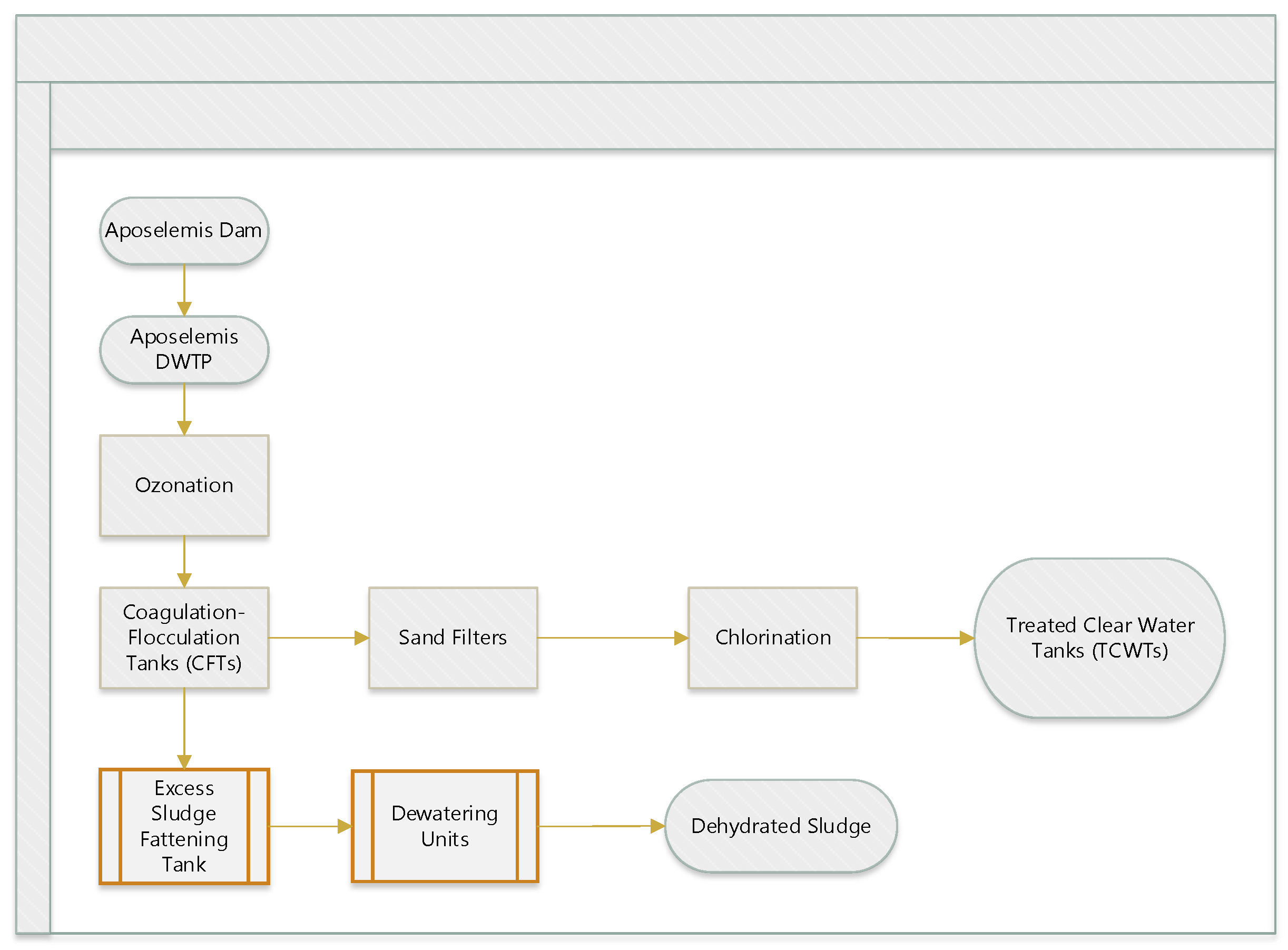
The Aposelemis Dam reservoir supplies drinking water to the northeastern part of Crete, Greece. The capacity of the reservoir is 25.3 × 10⁶ m³. Before entering the drinking water network, the surface water is treated at the Aposelemis DWTP to ensure compliance with high drinking water standards. First, the treated water is disinfected by ozone (in situ O₃ production), which also oxidizes the dissolved metals turning them into insoluble forms. Then, the alum coagulants and flocculants are added for the precipitation of the produced sludge. After that, the water passes through sand filters and undergoes final disinfection using chlorine gas (Cl_2(g)). A schematic of the treatment sequence is shown in Figure 1.

The Aposelemis DWTR has a maximum daily treatment capacity of 110,600 m³, although it usually operates at a third of its maximum capacity. The coagulant used at the DWTP is poly-aluminum chloride hydroxide sulfate (PACl). The quality of the produced drinking water meets the requirements of the drinking water legislation.

The processes of ozonation, coagulation, and disinfection are not easily simulated using classical modelling methods because of the complex physical and chemical mechanisms involved. Coagulation has been a common method for water treatment for decades; its main purpose is the removal of colloidal particles [12,17,27,29]. The steps followed during this study include: 1. collecting real operational data; 2. statistical analysis; 3. building; and 4. finally, selecting the ANN prediction model.

The basic statistics for the input and output parameters of the current study are given in

Table 1. Variables statistics.

No	Variable	Unit	Min	Max	Average	StDev
1	Daily difference in water height in reservoir (ΔH)	m	−1.91	3.55	0.00	0.18
2	Raw water supply (Q)	m3/d	4271	71,858	39,062	9492
3	Raw water turbidity (T1)	NTU	0.07	562.00	6.61	22.12
4	Raw water pH (pH1)		6.57	8.38	7.58	0.34
5	Treated water turbidity (T2)	NTU	0.01	0.74	0.16	0.08
6	Treated water pH (pH2)		6.42	8.03	7.30	0.32
7	Treated water residual chlorine (Cl2)	mg/L	0.02	0.90	0.44	0.11
8	Treated water concentration of aluminum (Al)	μg/L	7.00	146.00	41.97	21.36
9	Daily consumption of DWTP electricity (El)	kWh	1060	19,788	9424	2892
10	Residual O3 after ozonation process (O3)	mg/L	0.00	0.20	0.05	0.02
11	Anionic polyelectrolyte (ANPE)	mg/L	0.20	0.80	0.40	0.15
12	Poly-aluminum chloride hydroxide sulfate (PACl)	mg/L	7.00	100.00	17.99	11.64
13	Chlorine gas supply (Cl2(g))	kg/h	0.70	8.00	2.46	1.27
14	Filtration beds inlet water turbidity (T3)	NTU	0.17	7.25	1.29	0.84

.

2.2. Data Collection and Analysis

Water quality prediction models predict the water quality for future periods using historical data in real time and data from remote water quality monitoring systems [11]. According to the literature, although many efforts have been made to develop mathematical models to predict chemical usage in DWTPs, these models cannot predict the complex physicochemical processes in water treatment and may face difficulties analyzing the nonlinear relationships between process components, for example, in the coagulation process [12,29]. In order to obtain the input and output data that are required to develop and validate an ANN model, water analysis results were used from daily operational data for a period of 38 months (1,188 values for each of the 14 parameters for a total of 16,632 values). The data were either collected from the SCADA system through automated on- line analysis or through laboratory measurements according to standard methods and accredited ISO methods. The parameters analyzed in the lab were raw water turbidity (T1), raw water pH (pH₁), treated water turbidity (T₂), treated water pH (pH₂), treated water residual chlorine (Cl₂), treated water concentration of aluminum (Al), residual O₃ after the ozonation process (O₃), anionic polyelectrolyte (ANPE) dosage, poly-aluminum chloride hydroxide sulfate (PACl) dosage, filtration beds inlet water turbidity (T₃). The parameters of daily difference in water height in reservoir (ΔH), raw water supply (Q), daily consumption of DWTP electricity (El), and chlorine gas supply (Cl_2(g)) were obtained with the aid of sensors.

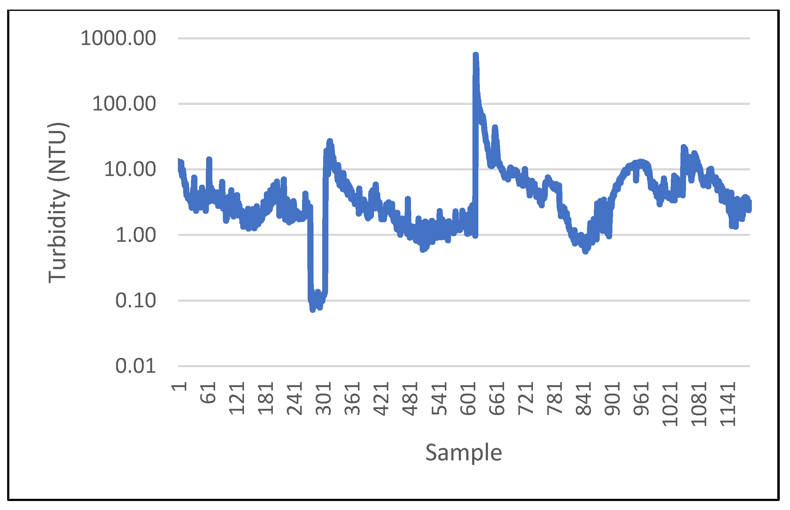
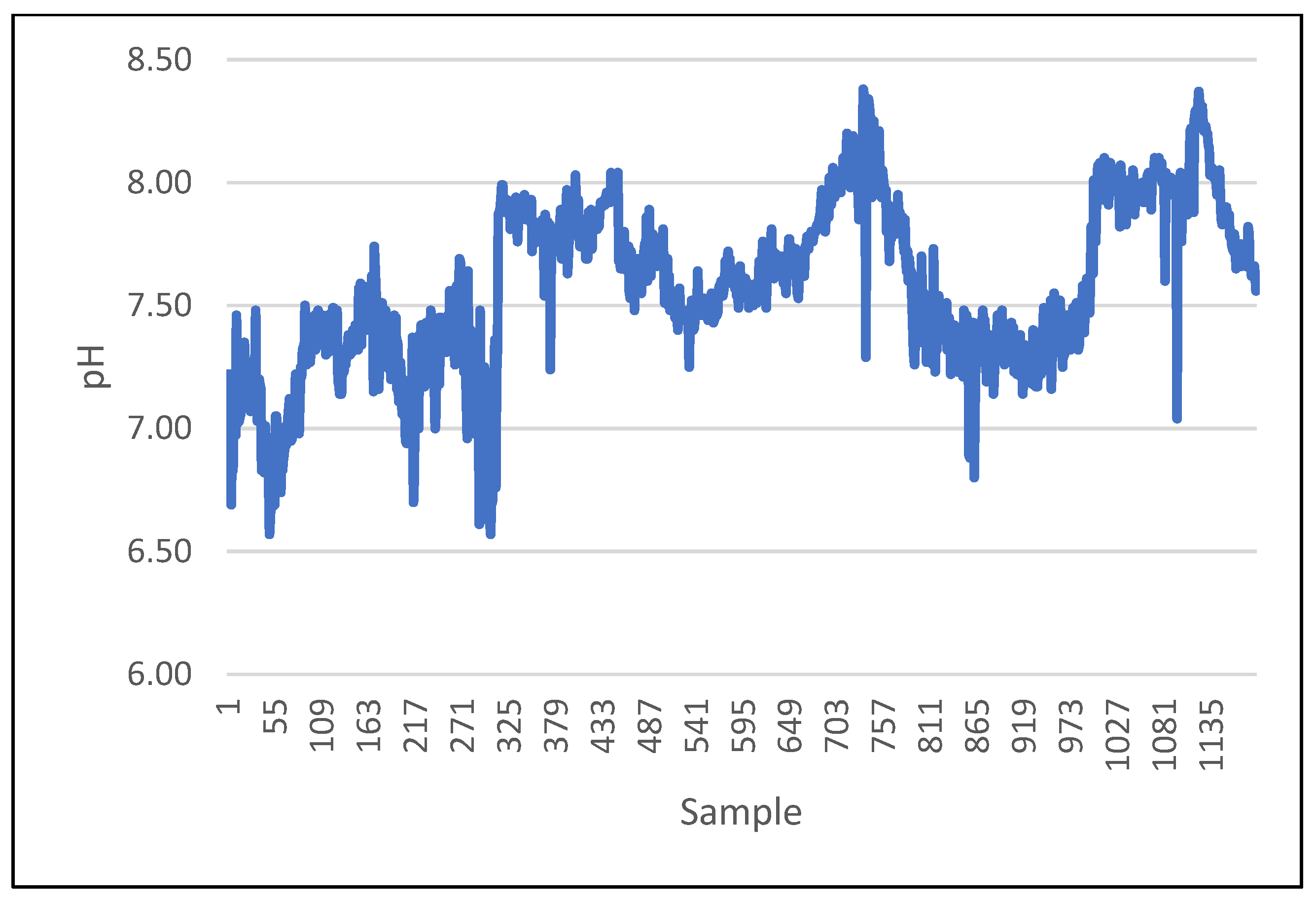
During data collection, seasonal variations in raw water quality data were observed. The fluctuations generally were minimal. However, during autumn and winter, which is the rainy season, increased variation in turbidity and pH value of raw water was observed. The progressions of the two main descriptors (raw water turbidity and pH) of the raw water quality over time are indicated in Figure 2 and Figure 3, respectively.

In order to use the data in the construction of the ANN models, data normalization was necessary because of the different ranges of scale among the different parameters. For this study, the input data of the ANN were normalized with final values between 0.0–1.0 by using the equation:

$$\mathrm{N}\mathrm{o}\mathrm{r}\mathrm{m}\mathrm{a}\mathrm{l}\mathrm{i}\mathrm{z}\mathrm{e}\mathrm{d} \mathrm{D}\mathrm{a}\mathrm{t}\mathrm{a}={\displaystyle \frac{\mathrm{L}-\mathrm{M}\mathrm{i}\mathrm{n}}{\mathrm{M}\mathrm{a}\mathrm{x}-\mathrm{M}\mathrm{i}\mathrm{n}}},$$

(1)

where L is the raw value, Max is the maximum value of raw value, and Min is the minimum value of raw value.

The ANN inputs consisted of ten (10) raw and treated water quality and operational data parameters: 1. raw water supply (Q), 2. raw water turbidity (T₁), 3. treated water turbidity (T₂), 4. treated water residual chlorine (Cl₂), 5. treated water concentration of residual aluminum (Al), 6. filtration beds inlet water turbidity (T₃), 7. daily difference in water height in reservoir (ΔH), 8. raw water pH (pH₁), 9. treated water pH (pH₂), and 10. daily consumption of DWTP electricity (El).

The ANN targets, factors needed to achieve the desired treated drinking water quality, were: 1. the residual ozone after ozonation process (O₃), 2. the anionic polyelectrolyte (ANPE) dosage, 3. the poly-aluminum chloride hydroxide sulfate (PACl) dosage, and 4. the chlorine gas supply (Cl_2(g)).

2.3. ANN Approach

Nineteen different ANN scenarios were examined using the Neural Fitting Tool (nftool) of MATLAB R2019a. In particular, 1188 values per variable were used with random division between training, validation, and testing procedures of the ANNs. The available data were divided into 70% for training (832 individual values), 15% for validation (178 individual values), and 15% for testing (178 individual values) of the developing ANN models. During training, the network used the training samples to adjust the weights, which connect the nodes, with the objective of minimizing the error between targets and simulated values. To avoid overfitting, the algorithm used early stopping, which makes use of the validation samples, and their respective error. When the validation samples error begins to rise while the training samples error continues to decrease, ANN generalization is considered to have converged and training stops. Other early stopping criteria also include a maximum number of epochs (to prevent infinite runs) and a minimum value of gradient (to avoid running after weight adjustments cease changing over time). Test samples have no effects on training or validation; thus, training error provides an independent measure of ANN performance and generalization ability.

For ANN training, the Levenberg–Marquardt Algorithm was chosen, since it is a fast-converging algorithm, widely used by the scientific community [30,31,32,33,34,35]. This algorithm typically requires more memory, but for this study, the memory needs did not exceed the specifications of a middle-range personal computer. The algorithm excels at minimizing the training errors of the ANN, but in order to avoid overtraining and to ensure the interpolating and extrapolating capabilities of the model, an early stopping mechanism was used. This early stopping mechanism used the validation dataset to check how the validation error evolves during training. Generally, the validation error decreases in the first iterations of the algorithm, and at a certain point reaches a minimum, and then starts increasing again, due to overtraining of the ANN. For the present work, training automatically stopped when the validation samples’ mean squared error increased for six (6) consecutive times, and the final ANN for that iteration was the one with the weights producing the minimum validation error. 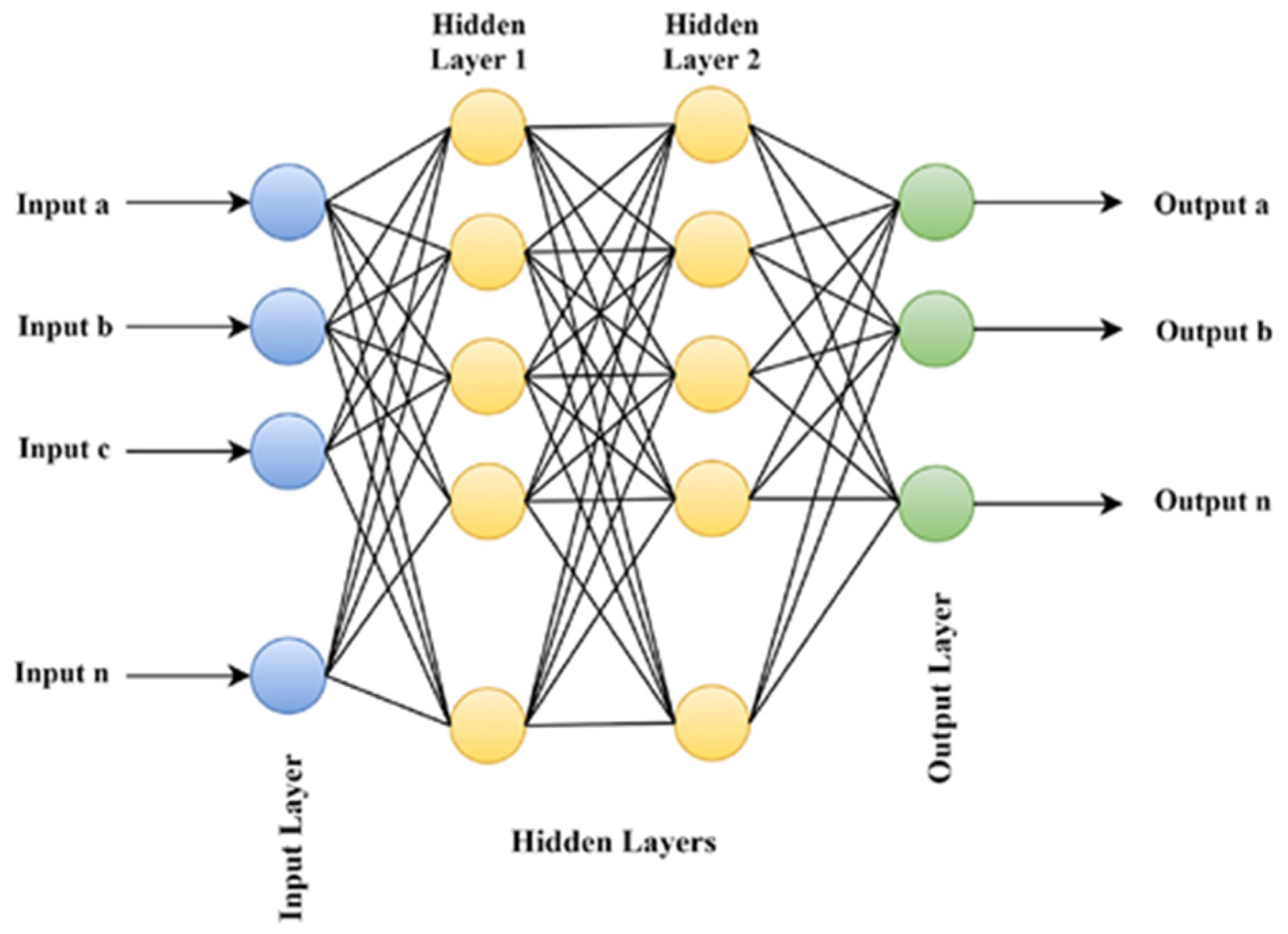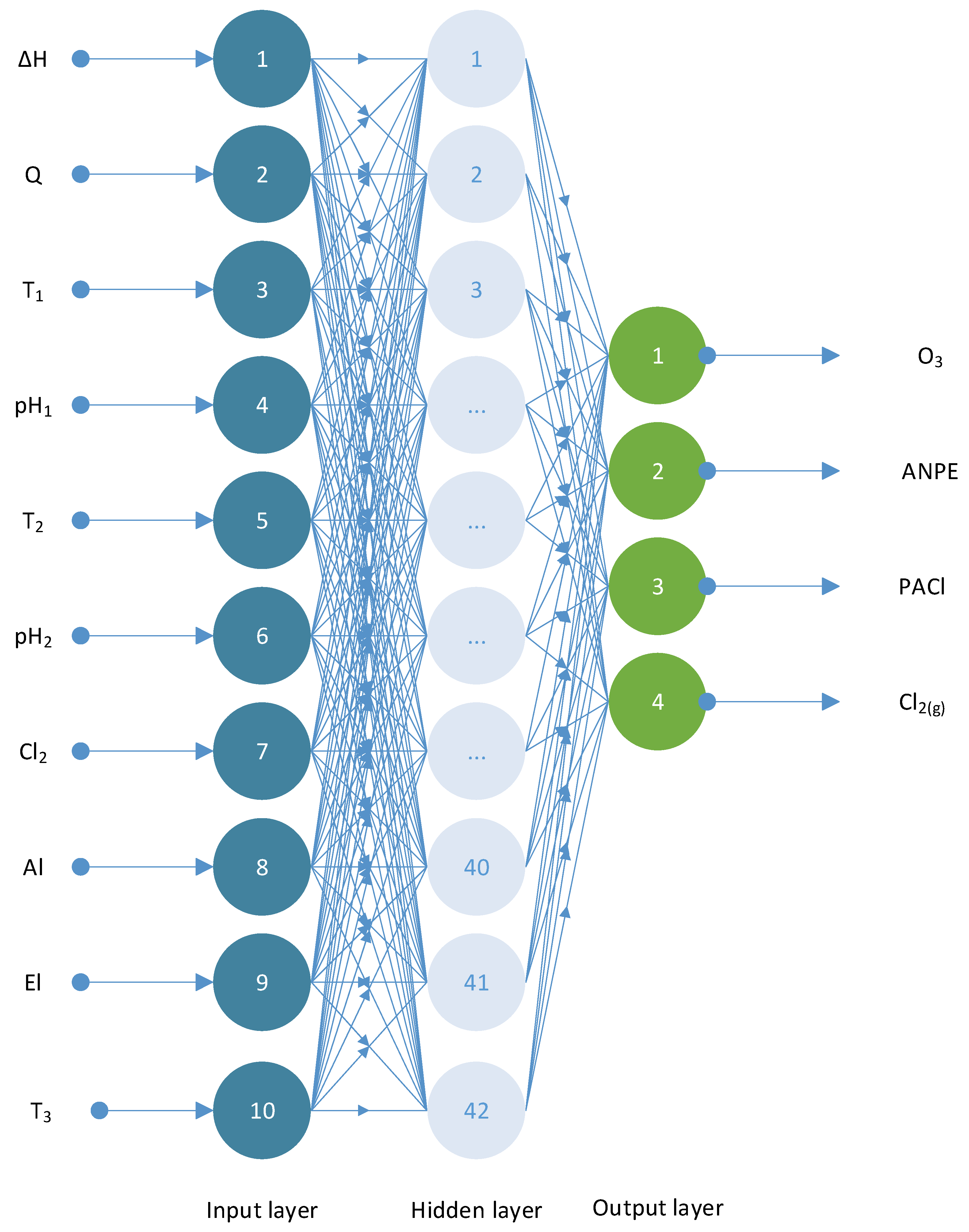Figure 4 shows the architecture of a simple ANN, which includes an input layer, two hidden layers, and an output layer [1,36].

Ensembles of ANNs were used instead of single ANNs in order to obtain more robust results. These ensembles consisted of many ANNs ranging from 10 to 100 ANNs in increments of 10 networks. Each ensemble had a maximum number of nodes for its ANNs, ranging from 10 to 100 maximum nodes in increments of 10 nodes. For each single ANN in any of these ensembles, the nodes of the hidden layer were subsequently randomly selected between one node and the maximum number of nodes in that specific ensemble.

Regarding the available data, the water quality and operational variables of the DWTP were categorized into three groups (

Table 2. Variables categorization.

No	Variable	Required to Be Present	Possibly to Be Necessary	Outputs
1	Daily difference in water height in reservoir (ΔH)		☑
2	Raw water supply (Q)	☑
3	Raw water turbidity (T1)	☑
4	Raw water pH (pH1)		☑
5	Treated water turbidity (T2)	☑
6	Treated water pH (pH2)		☑
7	Treated water residual chlorine (Cl2)	☑
8	Treated water concentration of aluminum (Al)	☑
9	Daily consumption of DWTP electricity (El)		☑
10	Residual O3 after ozonation process (O3)			☑
11	Anionic polyelectrolyte (ANPE)			☑
12	Poly-aluminum chloride hydroxide sulfate (PACl)			☑
13	Chlorine gas supply (Cl2(g))			☑
14	Filtration beds inlet water turbidity (T3)	☑

). The first category includes those variables that, based on the experience of the DWTP operators, are required to be definitely present as inputs to the ANN model. The variables included in the first category are: raw water supply (Q), raw water turbidity (T₁), treated water turbidity (T₂), treated water residual chlorine (Cl₂), treated water concentration of aluminum (Al), and filtration beds inlet water turbidity (T₃). The second group includes those variables that are possibly to be necessary as inputs to the ANN model. The variables included in the second group are: daily difference in water height in reservoir (ΔH), raw water pH (pH₁), treated water pH (pH₂) and daily consumption of DWTP electricity (El). The third group includes the variables as outputs to the ANN model. The parameters included in the third group are: residual ozone (O₃) after ozonation process, anionic polyelectrolyte (ANPE), poly-aluminum chloride hydroxide sulfate (PACl), and chlorine gas supply (Cl_2(g)).

2.4. MATLAB Code

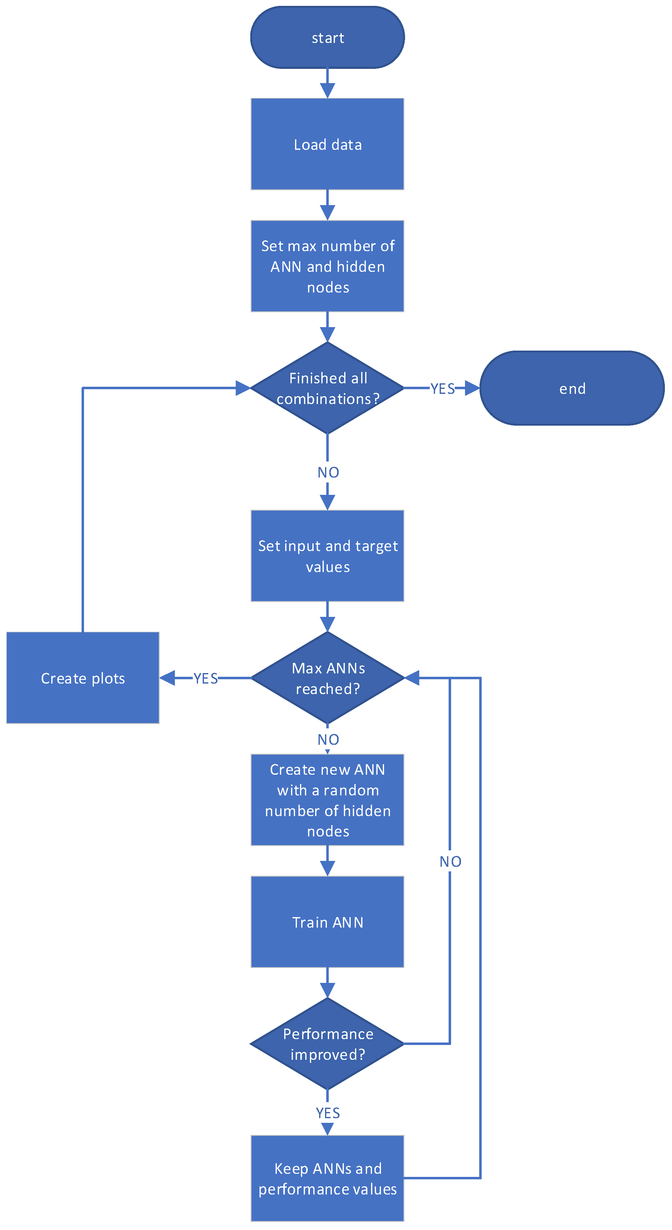
Appropriate code in MATLAB was designed and developed to run 16 different combinations of the 1st group variables combined with the 2nd group variables according to the canvas depicted in

Table 3. Different combination cases of 4 parameters that are possibly to be necessary.

AA	ΔH	pH1	pH2	El
1	1	1	1	1
2	0	1	1	1
3	1	0	1	1
4	1	1	0	1
5	1	1	1	0
6	0	0	1	1
7	0	1	0	1
8	0	1	1	0
9	1	0	1	0
10	1	1	0	0
11	1	0	0	1
12	0	0	0	1
13	0	0	1	0
14	0	1	0	0
15	1	0	0	0
16	0	0	0	0

. The flow chart of the algorithm (code) developed in MATLAB is depicted in Figure 5.

In this comparative study, we examined 19 different ANN scenarios based on the number of neural networks and the number of nodes, with 16 different combinations of variables (

Table 4. ANN Scenarios.

Nο	ANN Scenario	Neural Networks	Nodes	Variables Combination
1	NN10N10	10	10	16 different cases according to Table 2
2	NN20N10	20	10	16 different cases according to Table 2
3	NN30N10	30	10	16 different cases according to Table 2
4	NN40N10	40	10	16 different cases according to Table 2
5	NN50N10	50	10	16 different cases according to Table 2
6	NN60N10	60	10	16 different cases according to Table 2
7	NN70N10	70	10	16 different cases according to Table 2
8	NN80N10	80	10	16 different cases according to Table 2
9	NN90N10	90	10	16 different cases according to Table 2
10	NN100N10	100	10	16 different cases according to Table 2
11	NN100N20	100	20	16 different cases according to Table 2
12	NN100N30	100	30	16 different cases according to Table 2
13	NN100N40	100	40	16 different cases according to Table 2
14	NN100N50	100	50	16 different cases according to Table 2
15	NN100N60	100	60	16 different cases according to Table 2
16	NN100N70	100	70	16 different cases according to Table 2
17	NN100N80	100	80	16 different cases according to Table 2
18	NN100N90	100	90	16 different cases according to Table 2
19	NN100N100	100	100	16 different cases according to Table 2

) in each ANN scenario. In total, 304 different cases of ANNs were examined.

3. Results

3.1. Test Performance Indicator

Running 19 different ANN scenarios with 16 different cases per scenario (304 different cases), resulted in the creation of

Table 5. Best testing performance indicator per ANN scenario and case.

No	Neural Networks	Nodes	Case	Hidden Nodes	Outputs	Best t Perf	Time (s)
1	100	100	1	42	4	0.008848	23,346
2	40	10	7	8	4	0.008993	461
3	100	70	7	11	4	0.009211	10,383
4	100	50	13	46	4	0.009423	5860
5	100	20	4	13	4	0.009552	17,848
6	100	10	2	8	4	0.00957	801
7	100	80	6	72	4	0.009594	13,377
8	100	30	13	19	4	0.009642	2863
9	100	10	4	9	4	0.009658	801
10	100	60	1	12	4	0.009842	7898
11	100	30	1	8	4	0.009897	2863
12	80	10	1	8	4	0.009942	657

with the test performance (tperf) indicator values per scenario and case. Test performance (tperf) is the preferred performance indicator, since it is not biased, and the data used to calculate this were previously used neither for training nor for validation of the ANN. It is calculated as the Mean Squared Error (MSE) of the values in the test dataset. MSE is a statistical parameter and consists of the average squared difference between outputs and targets. The smaller the value of the tperf indicator, the better the performance, while zero values of the tperf indicates no differences at all. Table 5 includes only those scenarios with the minimum value of the tperf indicator, for the sake of brevity. The final selection of the optimum ANN model scenario is made among those with the smallest value of the tperf indicator.

The optimum selected scenario consisted of 100 neural networks, 100 nodes, 42 hidden nodes in 1 hidden layer, and belonged to case 1 [all 4 input parameters are selected (ΔH, pH₁, pH₂, El)].

3.2. Artificial Neural Network Model

The ANN model constructed with 10 Inputs (ΔH, Q, T₁, pH₁, T₂, pH₂, Cl₂, Al, El, T₃), 100 nodes, 42 hidden nodes and 4 Targets (O₃, ANPE, PACl, Cl_2(g)) is reflected in Figure 6. The suggested ANN model predict very well the studied main operational parameters.

A clear outcome of this analysis, as expected, was that as the number of neural networks increased, with fixed number of nodes (Nodes = 10), and as the number of nodes increased, with fixed number of neural networks (Neural Networks = 100), the running time of ANN models increased exponentially.

The results in Table 5 show that including all the measurable parameters in the prediction model improves its performance, but at the cost of increased processing time. Also, in Table 5, the second-best case is with two parameters fewer (case 7: pH₁, El parameters added and ΔH and pH₂ parameters are omitted by the prediction model) in a clearly much shorter time. This suggests that the relationship between ΔH and pH₂ parameters and the dosages of the chemicals that are used in a DWTP is much more complex, and only when a large number of neural networks is used can this complexity be captured.

Nevertheless, the ANN manages to reach the best test performance indicator to its minimum value. While the extra information provided by the two aforementioned parameters improves the selected prediction model accuracy by 1.65%, compared to the second-best scenario, it uses 42 hidden nodes versus 8 in a time of 23,346 s versus 461 s, respectively. Increasing the complexity of the ANN increases its accuracy, increasing the number of hidden nodes and ultimately the time required. In cases where time and computing power are important for decision making, a smaller number of neural networks and less complex models that can achieve satisfactory predictions are more desirable.

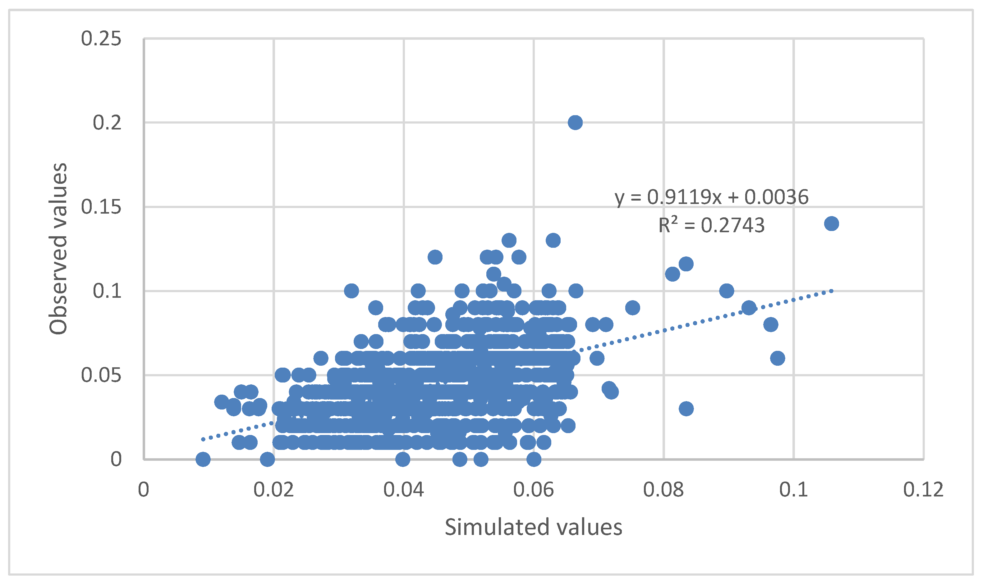
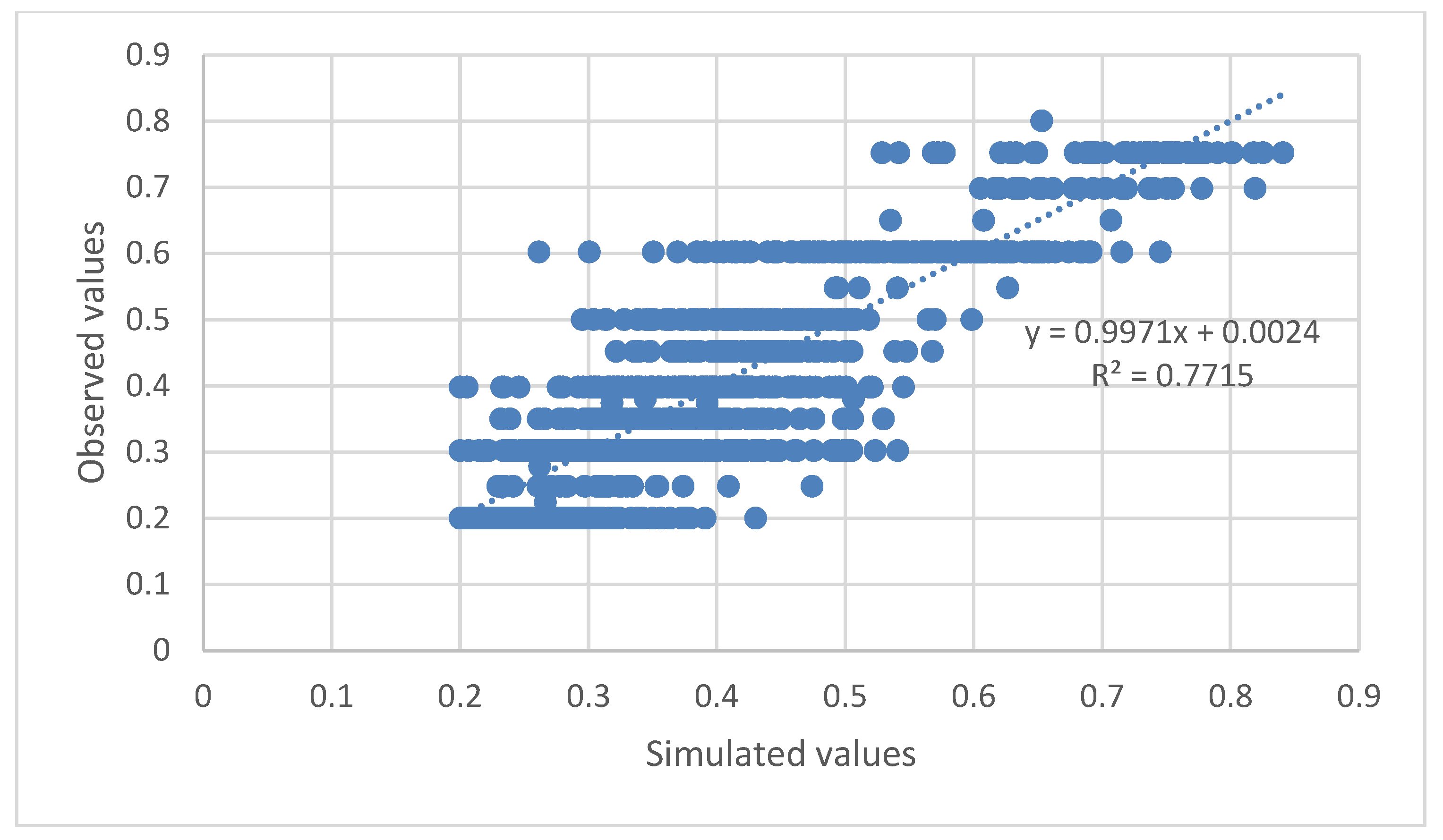
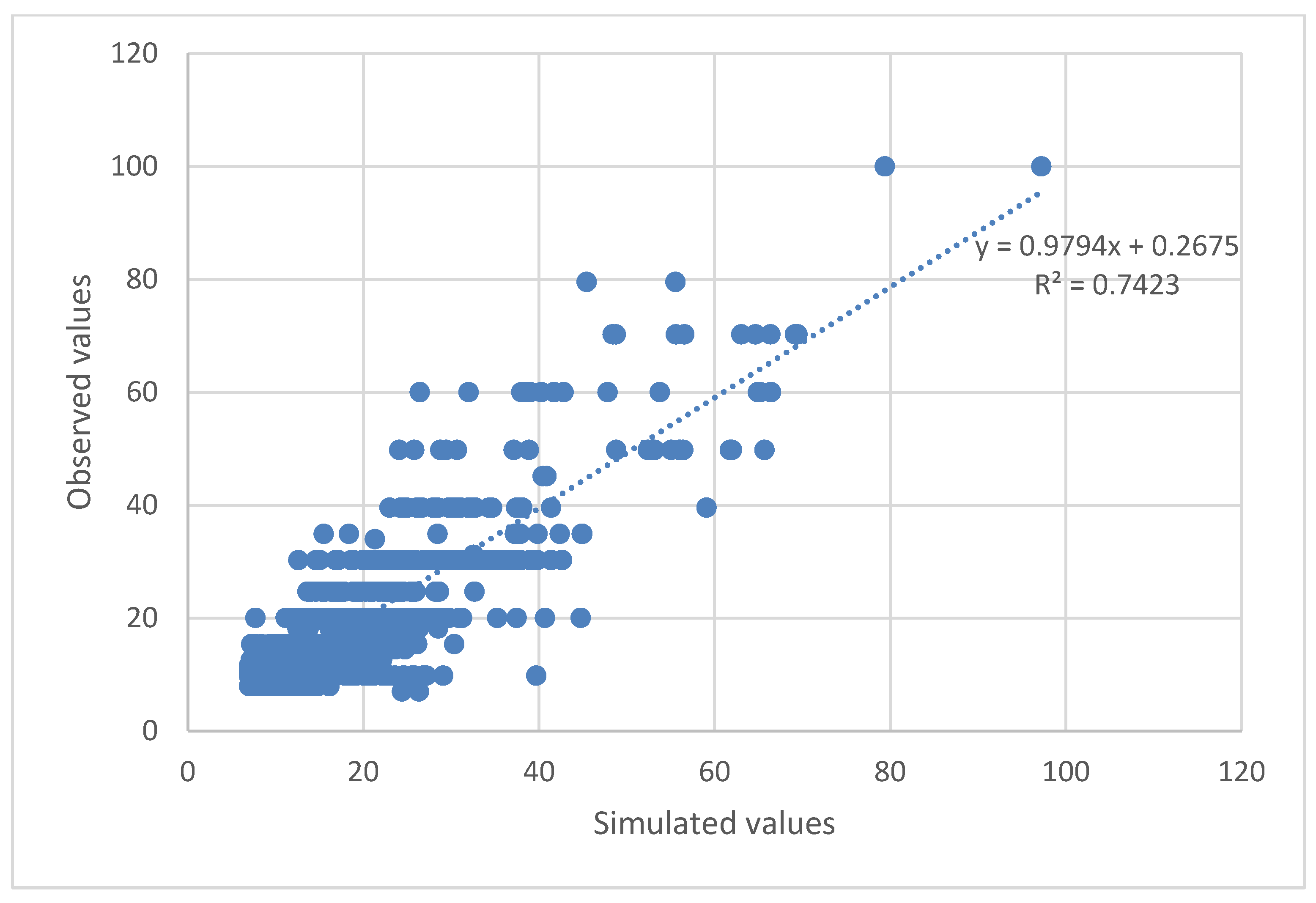
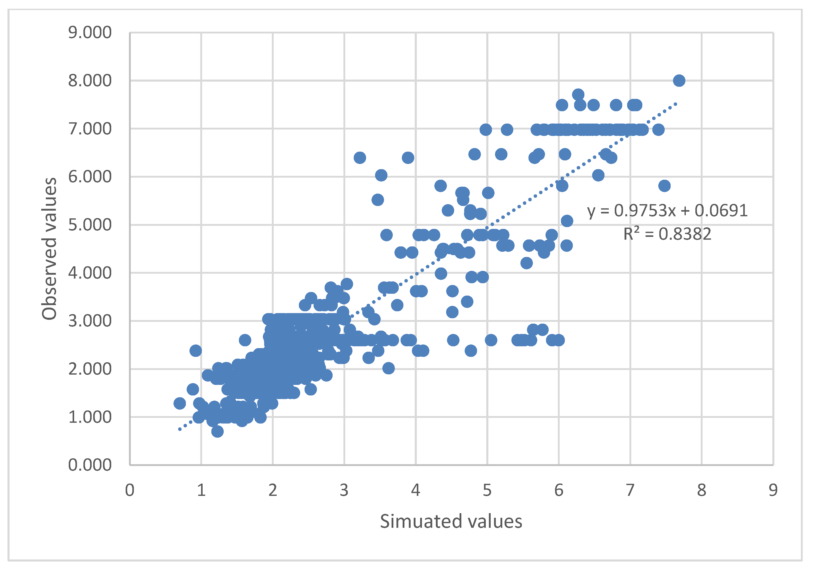
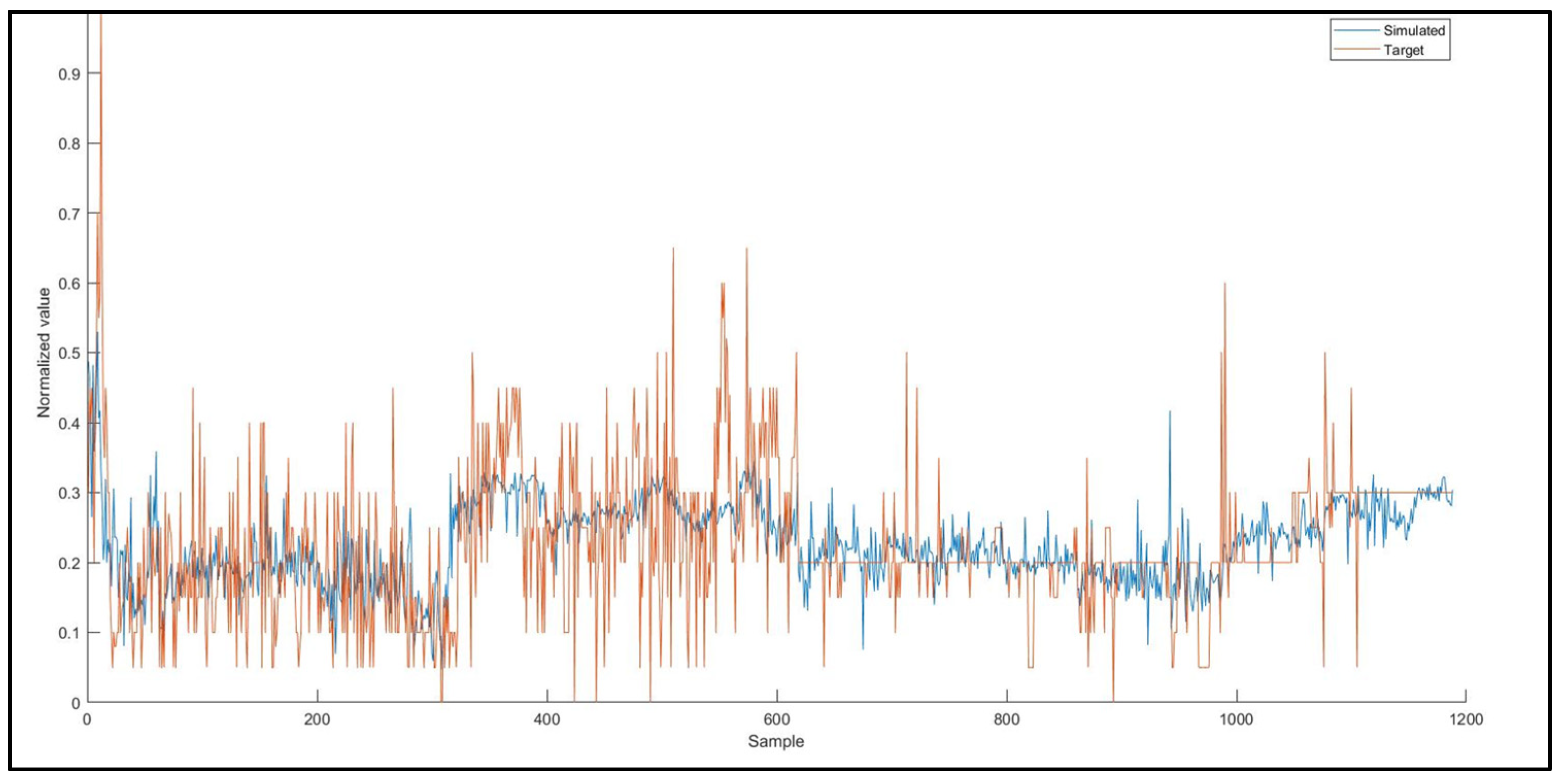
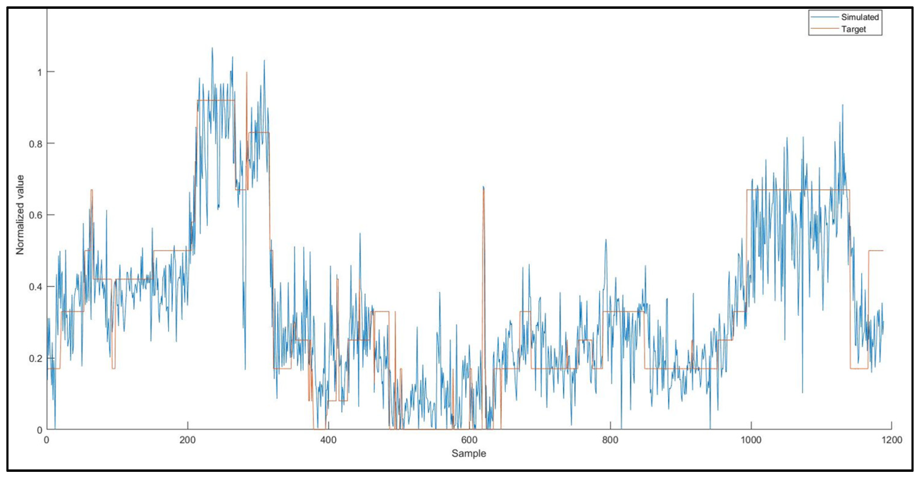
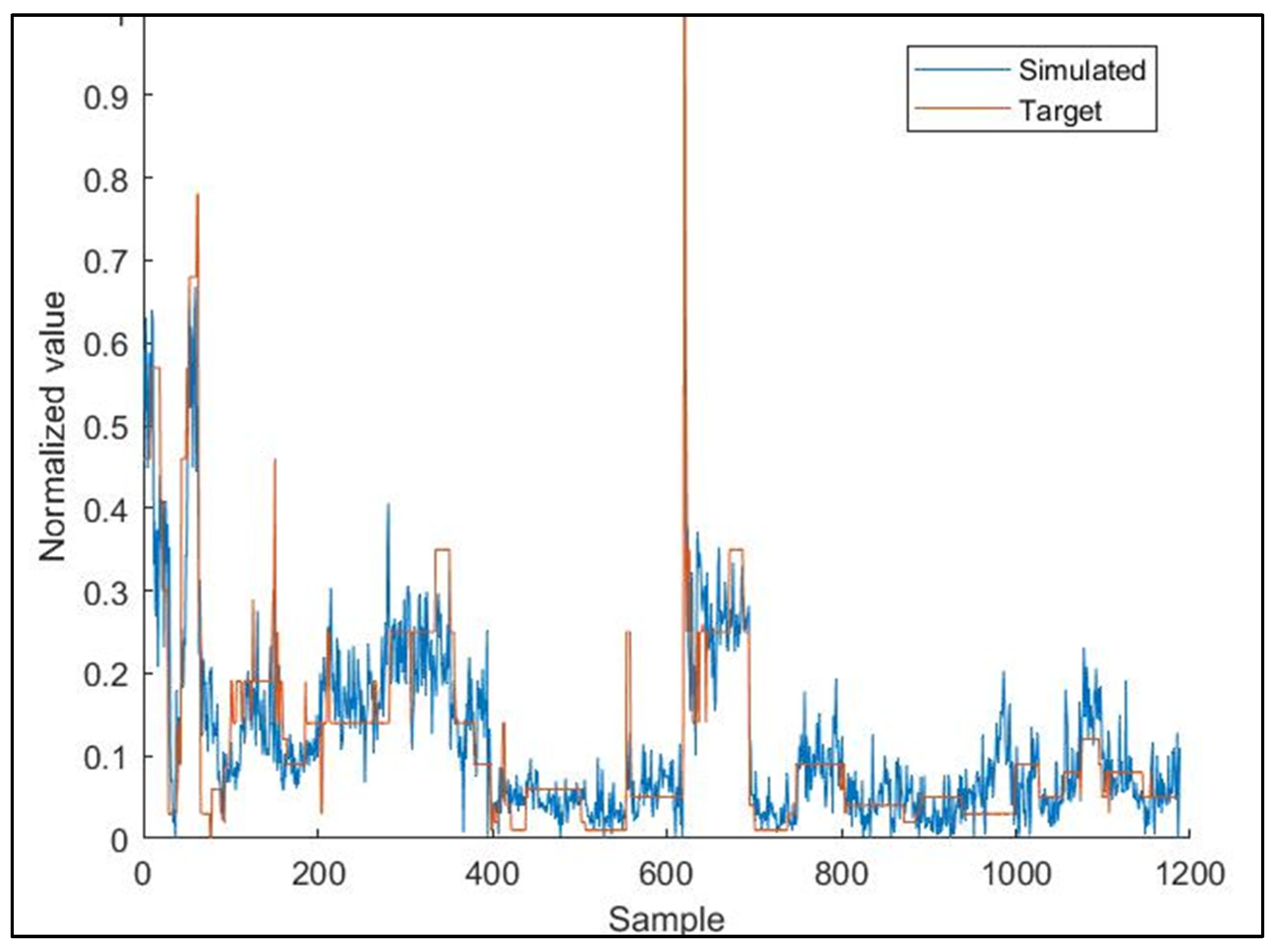
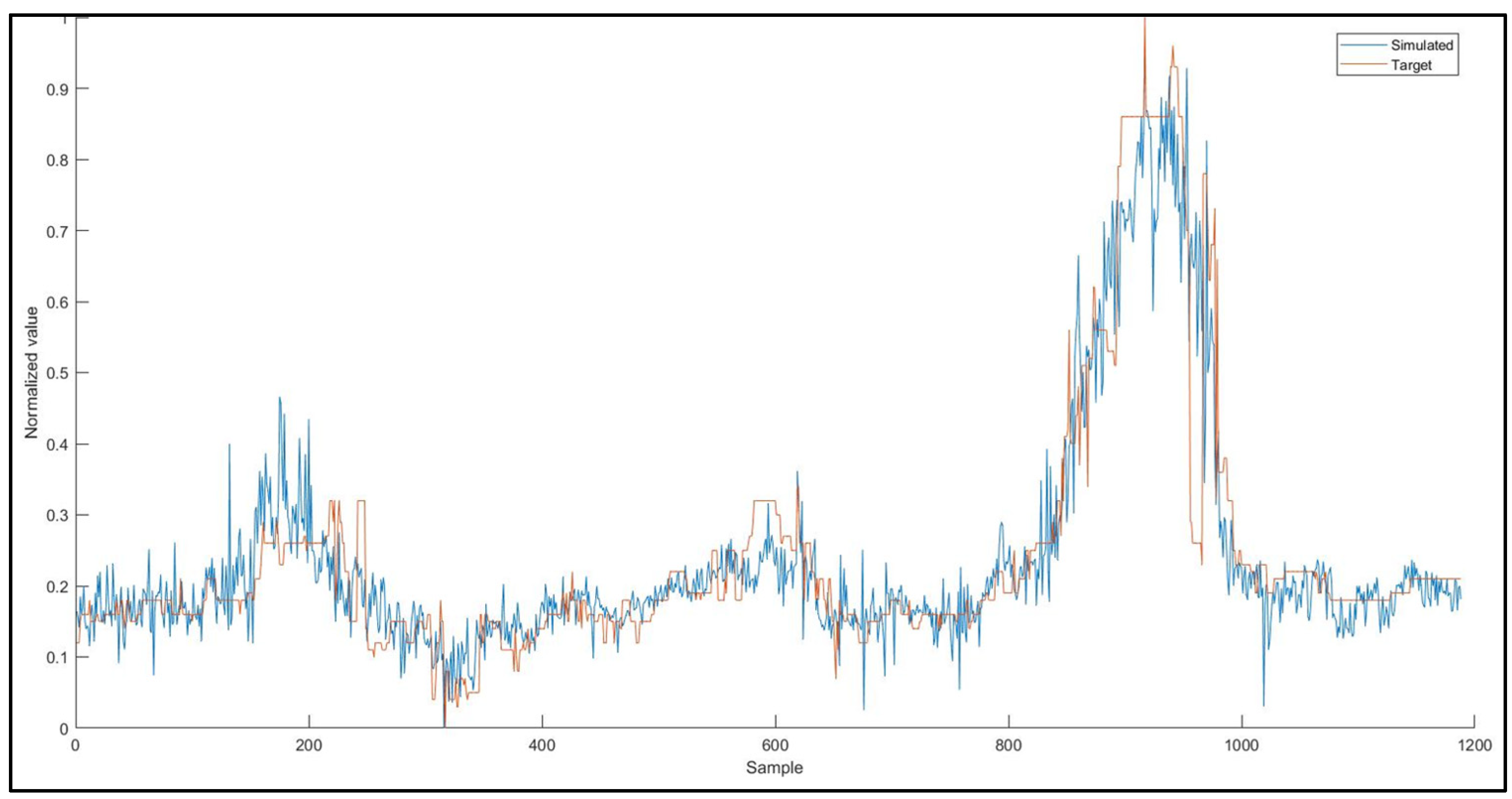
The plots between the normalized observed and model simulated values of the 4 target parameters, O₃, ANPE, PACl, and Cl_2(g) were constructed and are given in Figure 7, Figure 8, Figure 9 and Figure 10, respectively.

Figure 11, Figure 12, Figure 13 and Figure 14 show the simulated and observed values of the main operational parameters, which are the outputs of the developed ANN model.

Evaluating Figure 7, Figure 8, Figure 9 and Figure 10 and Figure 11, Figure 12, Figure 13 and Figure 14, one can easily conclude that the chosen ANN model satisfactorily predicts the values of the input parameters for the dosages of the chemicals used in the DWTP, with the exception of ozone dosage. It also follows the trend of increasing or decreasing them and satisfactorily approaches the extreme values to a large extent. The best value of R-squared (R²) is achieved for the Cl_2(g) prediction model, followed by ANPE, then by PACl, and finally by O₃. The wide variation of ozone values (see Figure 11) may justify the especially low value of R². According to the literature, an R² value greater than 0.5 is considered adequate for predicting sufficiently the values of input parameters [3,24,37,38,39]. The wide variation of ozone could be improved, in future studies, if a range of O₃ values were used rather than singly measured values.

For each of the four (4) ANN output parameters, the denormalization equations of the parameters (where NV: normalized value), are, respectively:

$${\mathrm{O}}_3=0.2\times {\mathrm{N}\mathrm{V}}_{{\mathrm{O}}_3}$$

(2)

$${\mathrm{S}\mathrm{P}}_{\mathrm{A}\mathrm{N}\mathrm{P}\mathrm{E}}=0.2+0.6\times {\mathrm{N}\mathrm{V}}_{{\mathrm{S}\mathrm{P}}_{\mathrm{A}\mathrm{N}\mathrm{P}\mathrm{E}}}$$

(3)

$${\mathrm{S}\mathrm{P}}_{\mathrm{P}\mathrm{A}\mathrm{C}\mathrm{l}}=7+93\times {\mathrm{N}\mathrm{V}}_{{\mathrm{S}\mathrm{P}}_{\mathrm{P}\mathrm{A}\mathrm{C}\mathrm{l}}}$$

(4)

$${\mathrm{S}\mathrm{P}}_{{\mathrm{C}\mathrm{l}}_{2\left(\mathrm{g}\right)}}=0.7+7.30\times {\mathrm{N}\mathrm{V}}_{{\mathrm{S}\mathrm{P}}_{{\mathrm{C}\mathrm{l}}_{2\left(\mathrm{g}\right)}}}$$

(5)

3.3. Case Study

Finally, we applied the selected ANN model, by using actual daily values of the operational variables of the Aposelemis DWTP (

Table 6. Case study inputs.

No	Input Variables	Unit	Value	Normalized Value
1	Daily difference in water height in reservoir (ΔH)	m	0.024	0.35
2	Raw water supply (Q)	m3/d	35,340	0.46
3	Raw water turbidity (T1)	NTU	7.85	0.01
4	Raw water pH (pH1)		7.9	0.73
5	Treated water turbidity (T2)	NTU	0.257	0.34
6	Treated water pH (pH2)		7.7	0.80
7	Treated water residual chlorine (Cl2)	mg/L	0.496	0.54
8	Treated water concentration of residual aluminum (Al)	μg/L	84	0.55
9	Daily consumption of DWTP electricity (El)	kWh	6269	0.28
14	Filtration beds inlet water turbidity (T3)	NTU	0.95	0.11

). The results of applying the selected model appear in

Table 7. Case study outputs of the best-performing ANN.

No	Target Parameters	Unit	ANN Model’s Predicted Values of the Target Parameters	Real Values Used in the DWTP
10	Residual O3 after ozonation process (O3)	mg/L	0.04	0.03
11	Anionic polyelectrolyte (ANPE)	mg/L	0.66	0.5
12	Poly-aluminum chloride hydroxide sulfate (PACl)	mg/L	11.05	10
13	Chlorine gas supply (Cl2(g))	kg/h	1.67	1.50

. The aim of the case study was to demonstrate how close the predicted values approach the values of variables chosen by the plant operators, based on their experience.

In comparing analyses from this specific case study and following the practices derived from the long-term experience of the plant operators, the differences between the quantities of chemicals actually used and those predicted by the ANN model were minimal. The forecast period is defined as the time during which the input values of the operational parameters in the chosen ANN model do not change significantly (±10%), e.g., seasonally, following severe weather events, after a significant change in the amount of water in the reservoir, etc.

The selected ANN model predictions could help plant operators optimize resource use, including reducing the consumption of chemicals and avoiding unnecessary tests. This leads to savings in both time and money while ensuring that the drinking water produced complies with the legal standards for human consumption.

4. Discussion

The present study reinforces the point of view that ANNs are useful tools for a DWTP, with high efficiency in complex relationship matching and forecasting. The conclusion that ANN models provide accurate prediction results has been drawn from many other similar studies [1,2,3,12,17]. In this study, the ANN model scenario finally chosen, from among the 304 examined scenarios, was the model with 100 neural networks, 100 nodes, and 42 hidden nodes. Specifically, the chosen ANN ensemble model was constructed with 10 input parameters (ΔH, Q, T₁, pH₁, T₂, pH₂, Cl₂, Al, El, T₃), 100 nodes, 42 hidden nodes, and 4 target variables (O₃, ANPE, PACl, Cl_2(g)). The choice was based on the smallest value of the tperf indicator. As expected, increasing the number of neural networks, with a fixed number of nodes, and increasing the number of nodes, with a fixed number of neural networks, result in an exponential increase in the running time of ANN models. Corresponding studies [4,11,14,15,16,17] have used similar raw water quality parameters (like pH, turbidity, and colour) with quite satisfactory results.

Incorporating all the available measurable variables into the prediction model improves its performance, though at the expense of time. On the other hand, the second-best case is with two parameters fewer (case 7: pH₁, El parameters are included and ΔH and pH₂ parameters are omitted) and reaches only slightly less satisfactory results, though in a clearly much shorter time. It is possible that the relationship between the ΔH and pH₂ parameters and the dosages of the chemicals used in a DWTP is much more complex, and only when a large number of neural networks is used, can this complexity be captured. It makes sense that the extra information, which is provided with the two aforementioned parameters, improves the selected model prediction accuracy by 1.65%. However, the slightly more accurate model uses 42 hidden nodes and takes 23,346 s, compared to the second-best scenario’s 8 hidden nodes and 461 s. As many studies have concluded [4,9,24,40], increasing the complexity of the ANN increases its accuracy, increasing the number of hidden nodes and ultimately the time required. In cases where time and computing power are important parameters for decision making, it appears that satisfactory results can be obtained using less complex models with fewer neural networks.

With the exception of the ozone dosage, the chosen ANN model effectively predicts the values of the input parameters for the chemical dosages used in the DWTP, which includes Cl_2(g), ANPE, and PACl dosages. It follows the trend of increasing or decreasing them and approaches the extreme values to a large extent. The value of R-squared (R²) is better achieved for the Cl_2(g) prediction model, followed by ANPE, then by PACl, and finally by O₃. The wide variation of ozone values may justify the specific low value of R². Corresponding studies have shown even better results regarding R² [7,9,17,24,40].

The ANN model is able to indicate the optimal Cl_2(g), ANPE, and PACl dosages, based on 38 months of measurement experience. In this way, the model’s predictions can assist new DWTP operators, in particular, in determining the required dosages of water treatment chemicals, thus saving time and helping them gain practical know-how. In the case of application at the Aposelemis DWTP, the facility operator will have a reliable estimation of the ANN output parameters, regarding the dosages of water treatment chemicals that should be applied, depending on the current quality and other available operational parameters. The suggested prediction ANN model responds satisfactorily in predicting the studied main operational parameters, as has been shown by similar studies [1,15,17,24,25].

Future research could focus on predicting DWTP chemical dosages using ANNs with a reduced number of operational parameters for greater flexibility, without prohibitively reducing the reliability of the prediction model. This could prove useful in cases with much larger numbers of samples, given that ANNs are highly data-demanding.