Article

Back-Calculation of Manning’s Roughness Coefficient by 2D Flow Simulation and Influence of In-Channel Physical Parameters in a Mountain River, Japan

1
Organization for Regional Co-Creation of Sustainable Communities and Watershed Disaster Resilience, Prefectural University of Kumamoto, 3-1-100 Kumamoto, Higashi-ku, Kumamoto 862-8920, Japan
2
River Planning Department, Nippon Koei Co., Ltd., 5-4 Kojimachi, Chiyoda-ku, Tokyo 102-8539, Japan
3
Faculty of Architecture and Civil Engineering, Kyushu Sangyo University, 2-3-1 Matsukadai, Higashi-ku, Fukuoka 813-8503, Japan
4
Laboratory for Watershed Disaster Resilience, Prefectural University of Kumamoto, 3-1-100 Kumamoto, Higashi-ku, Kumamoto 862-8920, Japan
*
Author to whom correspondence should be addressed.
Water 2024, 16(2), 320; https://doi.org/10.3390/w16020320
Submission received: 9 December 2023 / Revised: 6 January 2024 / Accepted: 13 January 2024 / Published: 17 January 2024
(This article belongs to the Topic Research on River Engineering)

Abstract

:
This study attempts to back-calculate Manning’s roughness coefficients by repeating a two-dimensional flow simulation to fit the spatially and temporally dense river water-level data observed in Japan’s Yamatsuki River, a typical mountainous river with an average riverbed gradient of 1/50 and an average river width of 17.9 m. Furthermore, we aim to clarify the influence of the in-channel physical parameters on the coefficient of roughness obtained through the above method. In the Yamatsuki River, 16 water-level gauges were installed at intervals of about 40~80 m in the longitudinal direction in the study reach. Manning’s roughness coefficients were back-calculated by repeating two-dimensional flow simulations to match the observed water levels of a flood in 2021 (the estimated maximum flow rate is 11.5 m3/s). The back-calculated roughness coefficients approached a constant value in the range of 0.05 to 0.1 s/m1/3 as the relative water depth increased, indicating that the roughness coefficient can be considered a constant value when performing plane two-dimensional flow calculations for flooding. The roughness coefficient during flooding was found to be correlated with the slope and step height (H)-step length (L)- channel slope (S) ratios (H/L/S). An equation for predicting the roughness coefficient during flooding based on the physical parameters of the channel is also proposed.

1. Introduction

Mountainous rivers are sources of flooding, sediment, and land-use disturbances [1,2] and are essential segments providing critical aquatic habitats [3,4]. There is a need to establish an integrated river management approach for mountainous rivers that implements flood protection while considering water and sediment continuity, biological habitats, and landscape. However, mountainous rivers flow quickly during floods and undergo large bed fluctuations, making field observations difficult. Consequently, primary field data and information on the geometry of the channel are lacking, and resistance characteristics such as the roughness coefficients of mountain river channels, which are essential for runoff analyses and riverbed fluctuation calculations in mountainous watersheds, are poorly understood.
A standard method for calculating the channel resistance of mountainous rivers is to establish several cross sections in the longitudinal direction of the river; determine the cross-sectional average velocity, water level, and flow rate in the study section at a specific rainfall event timing; and back-calculate Manning’s roughness coefficient n and Darcy-Weisbach’s friction coefficient f [5,6,7,8,9,10]. Asano et al. [5] organized the relationship between relative water depth and channel resistance using Manning’s roughness coefficient based on the previous literature. They reported that channel resistance, expressed as Manning’s roughness coefficient, converges to a constant value when the relative water depth exceeds 1. To back-calculate channel resistance, Comiti et al. [6] measured the flow and channel profiles in 10 reaches (slope 0.08 to 0.21 and length 16.1 to 76.4 m) of the Rio Cordon River with a catchment area of about 5 km2. The measurement section was set for each channel configuration to be obtained. Gabrielle et al. [7] calculated mean velocities using tracers for a total of 15 reaches (9 in the step-pool channel, 5 in the cascade channel, and 1 in the plane–bed channel) to determine channel resistance to outflow events from 0.28 m3/s to 0.68 m3/s. Reid et al. [8] established 13 basins in five tributaries with basin areas ranging from 12 km2 to 77 km2 and calculated the friction coefficient f by observing flow velocity and water depth during outflow events in 61 cross sections. Yochum et al. [10] estimated Manning’s roughness coefficient n and Darcy–Weisbach roughness in mountain rivers and reported that n ranged from 0.048 to 0.30 m1/3/s at high water and 0.057 to 0.96 m1/3/s at low flow. Marcus et al. [11] conducted a field study at Ptarmigan Glacier in the Juneau Icefield of Alaska with a mean precipitation of 2300 mm and slopes ranging from 0.02 to 0.16. Although the transect spacing was unknown, the authors reported that the flow rate during the observations ranged from 0.16 to 1.39 m3/s and the estimated roughness n ranged from 0.064 to 0.183 m1/3/s. Previous studies have also attempted to identify correlations between the calculated roughness or friction coefficients and hydraulic parameters, such as channel morphology, slope, and physical parameters, such as the grain size of the bed material and flow rate. The channel resistance of mountainous rivers under natural conditions not only varies spatially with channel morphology and gravel size [7,12] but also varies significantly with flow changes [5,10]. Montgomery et al. [12] showed that, for similar gradients, step-pool channels have higher roughness coefficients than plane–bed channels [13]. Yarahmadi et al. [14] analyzed laboratory data using soft computing models and indicated that the most important parameters affecting n were the energy grade line, the flow Froude number, the bed form dimensionless parameter.
As described above, field studies in various mountainous rivers have reported complex channel resistance in response to the complexity of channel geometry and flow fluctuations. However, the following issues remain. Since it is difficult to maintain uniform roughness conditions and channel geometry in mountainous rivers with complex channel geometries [11], to obtain a more accurate roughness coefficient, it is necessary to calculate roughness coefficients using spatially and temporally dense observed water-level data. However, observations of longitudinally dense data have rarely been conducted on mountainous rivers. Roughness coefficients for mountain rivers have been measured from low to very high flows, but little spatial variability has been reported. Takemura et al. [15] conducted 2D and 3D hydraulic analyses of a mountain river and reported that the possible roughness coefficients for 2D and 3D hydraulic calculations are different. Here, the three-dimensional calculations explicitly reflect the three-dimensional flow and non-hydrostatic distribution around boulders; the roughness coefficients representing the hydrograph converge to a constant value, while in the two-dimensional calculations, the roughness coefficients vary significantly from place to place. The authors noted that planar two-dimensional calculations cannot consider the three-dimensional flow and non-hydrostatic distribution around boulders. Additionally, the wrinkles are included in the roughness coefficients. However, although the reproducibility of the phenomenon is an issue for the roughness coefficient in 2D calculations, there is significant social demand for the roughness coefficient in planar 2D calculations, as models based on 2D calculations are widely used in practical applications from the perspective of computational resources.
This study attempts to obtain a roughness coefficient that fits the spatially and temporally dense river water-level data observed in Japan’s Yamatsuki River, a typical mountainous river, by repeating a two-dimensional flow simulation. Furthermore, we aim to clarify the influence of the physical parameters of the river channel on the coefficient of roughness obtained via the above exploratory method.

2. Materials and Methods

2.1. Summary of Methods

In the Yamatsuki River, a typical mountainous river in Miyazaki Prefecture, Japan, a 667 m section was established for analysis. In this section, 16 water-level gauges were installed at intervals of about 40~80 m in the longitudinal direction. The computed section was divided into sections, and Manning’s roughness coefficients were back-calculated by repeating unsteady two-dimensional flow simulations to conform to the results of water-level observations during flooding. The temporal variation of the roughness coefficient was also examined alongside the relative water depth, which is an important parameter. Several physical parameters of the river were extracted for the spatial variation of the roughness coefficient, and the relationship between the roughness coefficient and each parameter under high flow conditions was confirmed via a single correlation analysis. Multiple regression analysis was then conducted using Manning’s roughness coefficient as the objective variable and the physical parameters with high relationships as explanatory variables, and a prediction equation for the roughness coefficient was proposed.
Details of the survey methodology, survey items, and analysis methods are presented in the following subsections.

2.2. Study Field

The study site is a section of the Yamatsuki River, a tributary of the Gokase River that flows through Miyazaki Prefecture. Figure 1 shows the location of the Yamatsuki River. The Yamatsuki River is a typical mountainous river with a drainage area of 8.2 km2, a channel length of 4 km, an average riverbed gradient of 1/50, and an average river width of 17.9 m flowing through a valley. A 2.1 km span of the Yamatsuki River was damaged by Typhoon No. 14 in 2005 (Figure 2a). This flood caused significant damage, including the collapse of the revetment and the discharge of soil and sand from the rice paddies (Figure 2b).
After the flood of Typhoon No.14, river restoration was undertaken for flood protection and restoration of the river environment in response to residents’ opinions. At the time, there were many unknowns regarding mountainous rivers and no clear standards. Therefore, incorporating the opinions of river researchers, the river restoration was restored based on several innovations in addition to river flood calculations. The primary goal of the restoration was to restore the step-pool morphology (which is dominant in the riverbed morphology of mountainous rivers) to its natural state. To achieve this restoration, the river was not straightened but meandered, and the longitudinal gradient was maintained. Where the riverbanks were destroyed and the river’s width eroded, the river was kept widened, with the revetment using stones washed away by the flood. In addition, boulders larger than 1 m in diameter were left on the riverbed in anticipation of the formation of the step pool (Figure 2c). The restoration was completed in 2008. A follow-up survey conducted three years after the restoration reported the development of the riverbed’s topography and the recovery of plant and fish species [16].
For the study, we selected a 1190–1867 m section where the restorations were made, a 1 km section downstream of the river where the riverbed was not fixed by concrete, and a 677 m section where the influence of tributaries was minimal. In addition, the flow rate was expected to be somewhat constant.

2.3. Field Observations

The field survey consisted of continuously observing the water level using water-level gauges installed at 16 locations along the river in the study section and photogrammetric surveying using a UAV (Unmanned Aerial Vehicle).
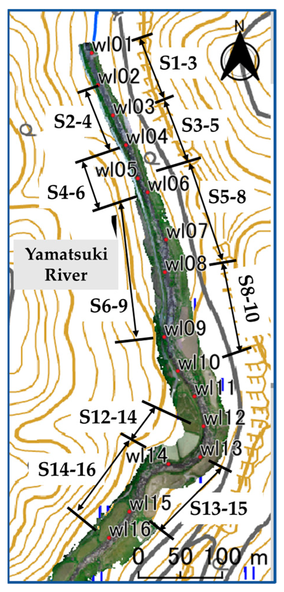
Pressure water-level gauges (HOBO U20L, Onset, USA 470 MacArthur Blvd., Bourne, MA, USA) were installed for the water-level observations. The observation period was from 6 August to 22 August 2021. The water-level gauges were installed by fastening the gauges to pegs with a cable tie and driving the pegs into the roots of huge rocks and gaps in the seawall. The water-level gauges were labeled wl01–wl16 with sequential numbers starting with the gauges installed downstream. A pressure gauge measuring atmospheric pressure was also installed near the river for compensation. Figure 3 shows the locations of the pressure gauges in plane view.
Topographic surveying was conducted with a UAV (Phantom 4 Pro V2.0, DJI) in April 2021 when topographic surveying was optimal because the river flow was low during the year. Aerial photographs were taken with Ground Control Points (GCPs) covering the entire study section. The aerial images were then used to obtain a 0.5 m resolution digital elevation model and orthographic projection map of the river channel via structure from motion (SfM) analysis using Metashape Professional ver. 1.7.1 (Agisoft).

2.4. Analysis Method

Many unsteady 2D flow calculations were performed while gradually changing the Manning’s roughness coefficient (given uniformly within a computed section), and the optimal Manning’s roughness coefficient that fit the water-level data obtained from the field survey was back-calculated. Ten computed sections were established so that each computed section contained three longitudinally contiguous water-level gauges, for each of which an inverse roughness estimation was performed using 2D flow calculations. Figure 3 shows the calculation sections. Based on the preliminary analysis, the back-calculated roughness coefficients for sections 9–11, 10–12, and 11–13 were excluded from the back-calculation analysis because there was no water depth response to roughness changes. The sections were located in a meandering section, so water depth was primarily determined by the large-scale river channel morphology not affected by local riverbed roughness.
The following sections describe the data sets, computational methods, and methods used for calculating the roughness coefficients and physical parameters required for unsteady 2D flow calculations.

2.4.1. Preparation of Data Set for Unsteady Two-Dimensional Flow Calculations

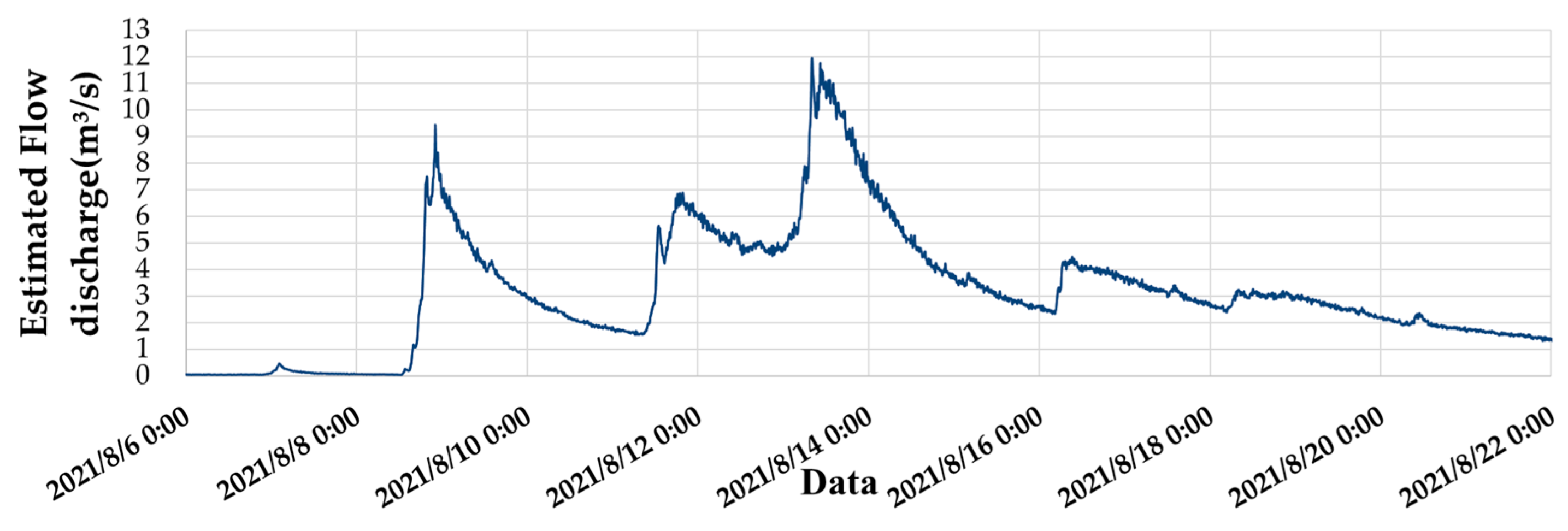
For the unsteady two-dimensional flow calculations, we used free software called iRIC Nays 2DH [17], which can capture nonlinear, unsteady hydrodynamics and subsequent bed and bank morphodynamics. The data required for unsteady 2D flow calculations were the water level at the upstream and downstream ends, the flow discharge, and the ground elevation. The pressure difference between the installed water-level gauge and a pressure gauge measuring atmospheric pressure was determined, and the longitudinal water depth was calculated from the pressure difference. Based on the river channel cross section and observed water levels, the flow discharge was estimated using the trapezoidal weir overflow Formula (1) for the cross section (at wl04 in Figure 4), where the exposed bedrock forms a drop-off structure and the dominant cross section is assumed to exist. The following equation was used to estimate the flow discharge based on data from erosion control facilities provided by the Ministry of Land, Infrastructure, Transport, and Tourism [18]:
Q = 2 15 C 2 g 3 B 1 + 2 B 2 h 3 2 ,
where Q is the estimated flow discharge (m3/s), C is the flow coefficient (0.6–0.66), g is the acceleration of gravity (9.8 m/s2), B1 is the width of the through-flow bottom (m), B2 is the overflow surface width (m), and h is the overflow depth (m). Figure 4 shows the estimated flow discharge. A maximum flow discharge of 11.5 m3/s was observed during the observation period. Since the maximum flow discharge calculated by David et al. [7], who previously analyzed relatively large rivers, was 0.68 m3/s, the roughness coefficients used in this study were considered sufficient to represent the flood. As the ground elevation data for the 2D flow calculations, we used a 0.5 m resolution digital elevation model obtained through photogrammetry.

2.4.2. Two-Dimensional Flow Calculation Method

(1)
Overview of the software (Nays2DH)
Nays2DH is a planar two-dimensional solver developed for river flow calculations. The flow field calculation model uses a general curvilinear coordinate system, which allows complex boundaries and riverbed topography to be directly considered. The friction on the bottom is evaluated using Manning’s roughness coefficient. The basic equations in Cartesian coordinate form (x, y) before mapping to the general curve coordinate system are shown below. The basic equations are taken from the solver manual [17]:
d h d t + d h u d x + d h v d y = 0
d u h d t + d h u 2 d x + d h u v d y = g h d H d x τ x ρ + D x F x ρ
d v h d t + d h u v d x + d h v d y = g h d H d y τ y ρ + D y F y ρ
τ x ρ = C f u u 2 + v 2
D x = d d x v t h d u d x + d d y v t h d u d y
D y = d d x v t h d v d x + d d y v t h d v d y
F x ρ = 1 2 C D a s h v u u 2 + v 2
F y ρ = 1 2 C D a s h v v u 2 + v 2 ,
where h is water depth; t is time; u and v are depth-averaged velocities in the x and y directions, respectively; g is the acceleration of gravity; H is the water level; τx and τy are the riverbed shear forces in the x and y directions, respectively; ρ is the density of water; Dx and Dy are diffusion terms in the x and y directions, respectively; Fx and Fy are the resistance forces of the plant in the x and y directions, respectively; Cf is the riverbed shear coefficient; vt is the eddy kinematic viscosity coefficient; CD is the drag coefficient of the plant, as is the intercepted area of the plant in unit volume; and hv is the smallest plant height and water depth. Using the above equations as a basis, the calculation mesh can be set to any shape by converting it into general coordinates.
(2)
Calculation conditions
In the present study, the resistance forces of the plant were specified as zero, which is reflected in the roughness coefficient. “+Advanced” was selected as the solver type for the calculation conditions. The calculation time step was determined by considering the Courant number derived from the following equation:
C = v Δ t Δ l ,
where C is the Courant number, v is the flow velocity, Δt is the computation time step, and Δl is the grid size. The Courant condition requires that the Courant number be smaller than 1 for a stable analysis. The computation time step was set to 0.01 s to satisfy the Courant condition. Isocurrent calculations gave the initial water surface profile, and the number of CPUs used for parallel calculations was set to 8, with default values for other settings.
Ten calculation sections were established with three longitudinally contiguous water-level gauges. The water-level gauge wl07 was washed out through the flood. Therefore, the river was divided into calculation sections at the 15 water-level gauge locations from which the water-level data were obtained (Figure 3). The section names are given by the numbers of the water-level gauges located at the downstream and upstream ends of the section. For example, if wl01 is located at the downstream end and wl03 at the upstream end, the section is named section “S1–3”. The 0.5 m ground elevation obtained from the field survey was used to create the computational grid, and the mesh size was also set to 0.5 m. The center line of the river channel and the right and left bank lines were created according to aerial photographs taken by the Geospatial Information Authority of Japan (GSI). The “Generic Lattice Generation Tool” was employed as the lattice generation algorithm, which solved the Laplace equation to generate a smooth lattice. The lattice was created so that the lattice points would overlap with the water-level gauge locations in the middle of the section. This arrangement allowed us to compare the observed and calculated water levels at the water-level gauge locations.
(3)
Boundary conditions
Ten time series data with varying flow levels were extracted for 2D flow calculations and roughness estimation to obtain roughness coefficients for each runoff phase. For each time series data, 2D indeterminate flow calculations were performed using the upstream end discharge data and downstream end water-level data for 10 min as boundary conditions for the time series data. To stabilize the calculations, an additional 10 min steady flow calculation was performed at the beginning of the calculation using the initial flow and water level values, followed by the 10-minute unsteady flow calculation. Table 1 shows the hydraulic boundary conditions for the periods used in the calculations.
(4)
Back-calculation of Manning’s roughness coefficient
In this study, Manning’s roughness coefficient was back-calculated using the local indeterminate flow back-calculation method. In this method, the river channel is divided into several sections, and the roughness coefficients of each section are changed by trial and error to calculate the indeterminate flow. The Nays2DH solver in iRIC was used for the unsteady two-dimensional flow calculations. The Manning’s roughness coefficients ranged from 0.1 to 1 in increments of 0.1, and calculations were performed by further varying the coefficients at intervals of 0.01 between values that were close to each other. The calculated and observed water levels were compared; the result with the smallest difference between the calculated and observed water levels was used as the Manning’s roughness coefficient for that section. In this study, we calculated 10 times × 10 sections x 20 times the number of trials = 2000 patterns. The iRIC project data were recorded in the CGNS file format, which is used in computational fluid dynamics, making it challenging to edit the data directly. The PyAutoGUI library in Python was used to create project files with different conditions in RPA. The roughness coefficient for the calculation pattern with the most minor difference between the calculated water depth obtained from the simulation in the section and the observed water depth was determined as the back-calculated roughness coefficient.
(5)
Accuracy verification
To confirm the accuracy of the unsteady two-dimensional flow calculation simulation, a comparison was made between the water depth obtained from the flow observations and the calculated water depth obtained from the simulation. Table 2 shows the mean squared error between each section’s calculated and observed water levels for the back-calculated roughness coefficient. Here, the mean squared error is small, indicating that the calculated water level accurately reproduced the observed water level when the back-calculated roughness coefficient was used (see also Table 2).

2.4.3. In-Channel Physical Parameters Related to the Roughness Coefficient

Previous studies have reported that riverbed roughness varies with water depth [19]. Indeed, roughness is expected to vary with water depth, even in unsteady two-dimensional calculations. To calculate Manning’s roughness coefficient during a flood, we compared the roughness coefficient and relative water depth at each of the times indicated in the boundary conditions, with reference to previous studies. The relative water depth was calculated by dividing the water depth by D84, which was obtained from the grain size accumulation curve. From among the ten values set as boundary conditions, water depth under maximum flow was used. The D84 grain size of the riverbed material was calculated by creating a grain size distribution curve using the image-based line grid method.
In predicting the back-calculated roughness coefficient during flooding based on the abovementioned physical channel parameters, the following relevant channel physical parameters were selected: river ratio of width to depth, slope, D84 grain size of riverbed materials, relative water depth, ratio of plants, ratio of habitat per section, and H/L/S (H: step height; L: step length; S: channel slope). H/L/S, as proposed by Abrahams et al. [20], is widely used to test the occurrence of the maximum flow resistance condition in mountainous streams. These parameters were calculated using QGIS 3.1.6 with a 0.5 m grid DEM and ortho imagery.
The width-to-depth ratio was selected as a dimensionless value divided by the water depth to assess the extent to which the river width, a parameter that can be controlled during design, affects the roughness coefficient. The width–depth ratio was calculated by dividing the river’s average width by the river’s depth. The average river width per section was divided into five equal sections, and the average value was used as the average river width. The water depth was selected as the water depth value when the relative water depth reached its maximum value. Gradient and relative water depth values were selected because they were related to the roughness coefficients of mountainous rivers in previous studies [5]. The slope was calculated by dividing the channel length at the upper and lower ends of each set section by the difference in elevation between the upper and lower ends, i.e., channel length/elevation difference = slope. The relative water depth was calculated for each of the ten time periods described above, and the value with the most significant back-calculated roughness coefficient was selected. The D84 grain size of the riverbed material, ratio of habitat per section, and maximum flow resistance index H/L/S were selected as parameters to investigate the effectiveness of the step-pool as the main roughness factor for mountainous rivers, which was already known from existing studies. The ratio of habitat, as an occupation of each habitat in each section, was calculated by classifying the river channel into four habitats: step, pool, rapid, and riffle. In the field, we classified step-pools, characteristic river bed forms in mountain river channels. During the step-pool sequence, we classified areas with little wave action as riffle and areas with fast flow and whitecaps as rapid. For each habitat roughly classified during the field survey, polygons were created using ortho-images in GIS 3.2 software. The ratio of each habitat was calculated by dividing the polygon area of each habitat by the area of each section.
H/L/S is calculated as H: step height, L: Step length from the step to the end of the pool, and S: section longitudinal gradient. A longitudinal gradient was created from the obtained ground elevation, and the average value of H/L/S was calculated for each set section. The ratio of plants, as an area occupation of plants in each section, was selected based on the expectation that the effect of the plant would be included in the roughness coefficient since the plant density term was omitted in the unsteady two-dimensional flow calculation in this study. The distribution of vegetation in the Yamatsuki River is closely related to the development of troughs (Sato, unpublished data) and should be interpreted as implicitly including the effects of flow inhibition by troughs. Polygons surrounding the plant areas were created using ortho-images in GIS software. The ratio of plants was calculated by dividing the polygon area of plants by the area of each section.

2.4.4. Regression Analysis to Examine In-Channel Physical Parameters Most Strongly Affecting the Roughness Coefficient

A single regression analysis between the physical parameters described above and Manning’s roughness coefficient was applied to investigate the factors influencing the back-calculated inverse roughness coefficient. The corresponding data set is shown in Table 3. In addition, multiple regression analysis was conducted to develop an equation to predict Manning’s roughness coefficient in mountainous rivers, selecting the physical parameters with significant correlation coefficients.

3. Results and Discussion

3.1. The Back-Calculated Manning’s Roughness Coefficients and Their Relationship with the Relative Water Depth

We were able to observe spatially and temporally dense water-level data for a mountainous river and back-calculated Manning’s roughness coefficients at various discharge stages using several results from two-dimensional flow calculations. Since it is known from previous studies that the coefficient of roughness varies with changes in flow rate, we first estimated the final coefficient of roughness during a flood event and then assessed whether the coefficients differed from section to section.
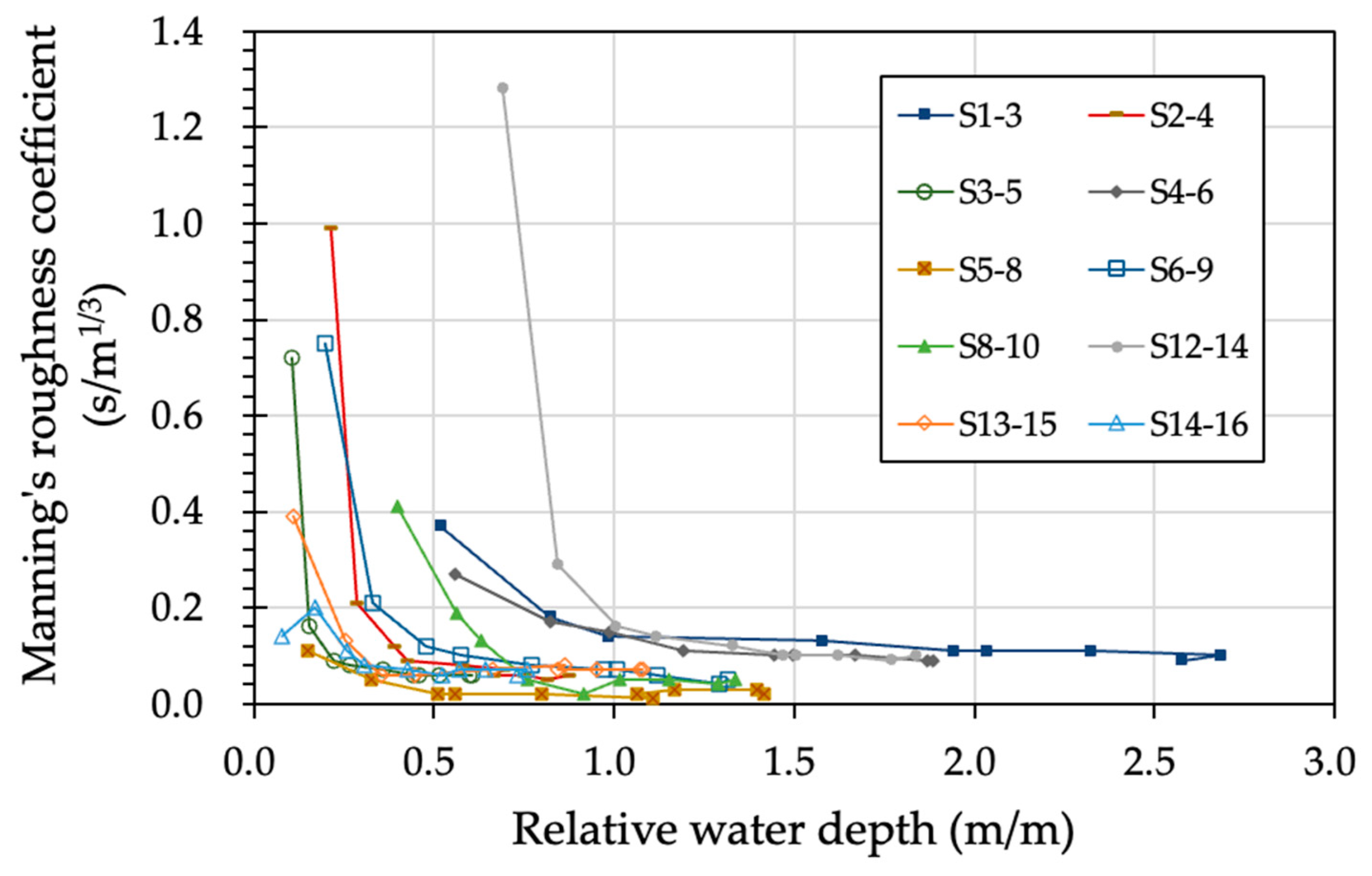
The relationship between the obtained back-calculated roughness coefficients and relative water depths are shown in Figure 5. The Manning’s roughness coefficients ranged from 0.11 to 1.28 m1/3/s in the early stages of computation in each computed section, i.e., when the riverbed gravels were not submerged in the early stages of the flood. In particular, sections 2–4 and 12–14 had coefficients of roughness greater than 0.96, with values exceeding the range of 0.057 to 0.96 m1/3/s reported by Yochum et al. [10] for roughness under a low flow. As the relative water depth increased, Manning’s roughness coefficients generally reached their maximum when the relative water depth fell within the range of 0.5 to 0.1 m1/3/s. Asano et al. [5] reported a minimum roughness coefficient of 0.16 m1/3/s for the step pool, Montgomery et al. [12] reported a roughness coefficient of 0.1~0.2 m1/3/s for the step pool, and Yochum et al. [10] reported a coefficient of 0.048~0.3 m1/3/s for high water. Therefore, we maintain that a Manning’s roughness coefficient with a high relative water depth is generally reasonable.
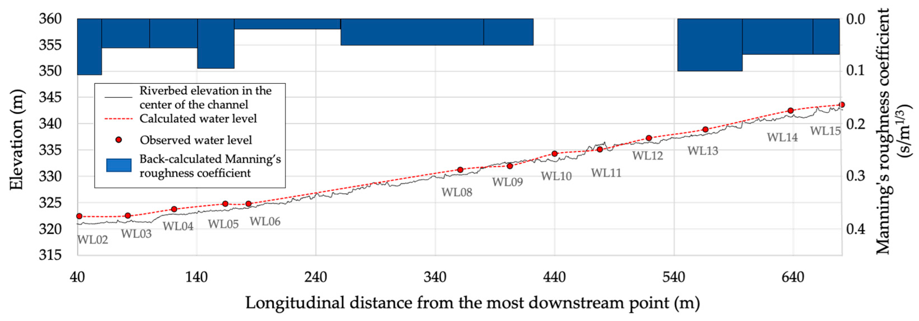
Step height significantly correlates with the D₅₀ and D₈₄ values of the constituent gravel diameter [21]. Since the relative water depth in this study is assumed to be h/D₈₄, the step is expected to be submerged below the water surface where the relative water depth exceeds 1 [21,22]. Asano et al. [5] reported that Manning’s roughness coefficient calculated from steady flow calculations converges to a constant value with an increase in relative water depth. This study calculated the roughness coefficient backward from unsteady two-dimensional flow calculations for each section. The results confirmed that Manning’s roughness coefficient decreases with an increase in relative water depth and converges to a constant value. However, Manning’s roughness coefficient was found to vary from section to section. The longitudinal distributions of the back-calculated roughness coefficient, calculated water level, and observed water level at peak flow (i.e., when the relative water depth is maximum) are shown in Figure 6. It is suggested that the convergence of Manning’s roughness coefficient may change depending on the river channel’s spatial factors and physical parameters.

3.2. Effects of In-Channel Physical Parameters on the Roughness Coefficient

Single regression analysis was performed to clarify the relationship between the physical parameters and roughness coefficient. In the single regression analysis, Manning’s roughness coefficients at the maximum relative water depth were used to represent channel resistance during the flood. The results are shown in Figure 7. Furthermore, multiple regression analysis was performed between the parameters with the strongest correlation and Manning’s roughness while considering multicollinearity.
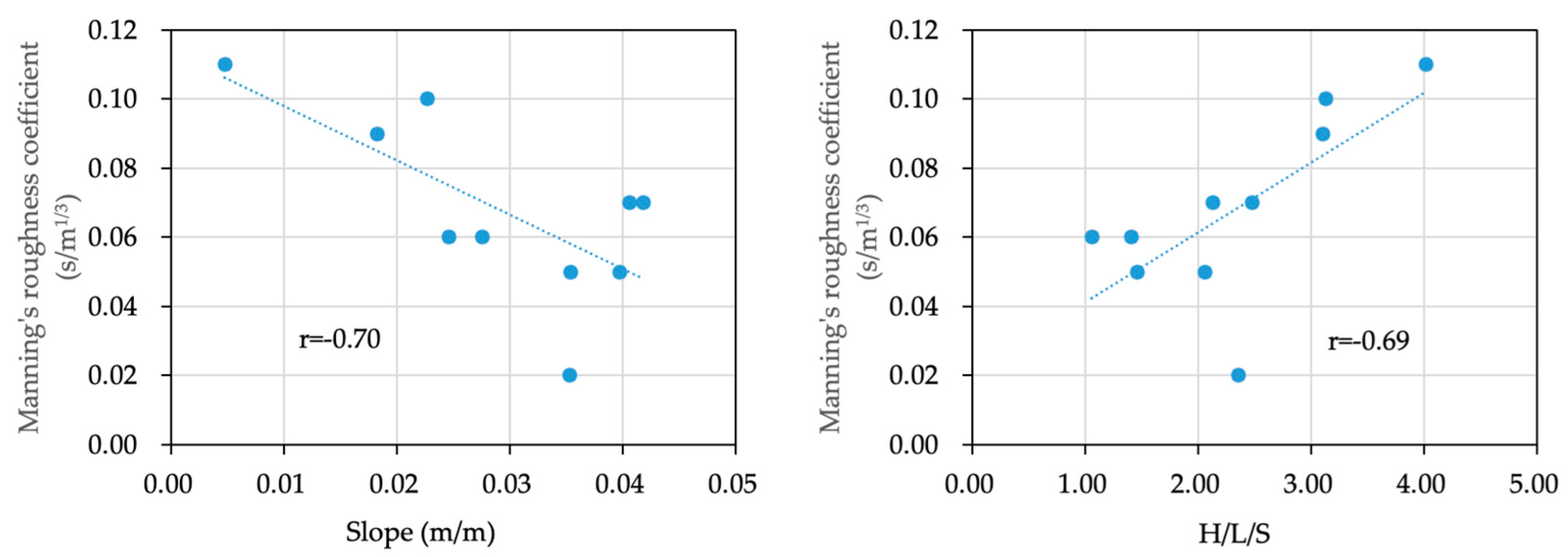
The previous section confirmed that Manning’s roughness coefficient during a flood with high water levels is spatially varied. Figure 7 shows that the slope was negatively correlated with Manning’s roughness coefficient, and H/L/S was selected as the positively correlated parameter. On the other hand, the ratio of width to depth, D84 grain size of the streambed material, relative water depth, plant rate, and habitat ratio per section did not correlate well. The D84 grain size of the riverbed material and the ratio of habitat per section were selected to explain the effects of the step pool in dispersing the energy of the flow, and H/L/S, which was selected for the same reason, had a high correlation. Thus, H/L/S was selected as the number to express the step pool for the roughness coefficient. H/L/S is likely the most appropriate number to express the step pool for the roughness coefficient. Manning’s roughness coefficient, calculated using a planar two-dimensional calculation, expresses the effects of friction roughness and shape roughness. The river roughness is considered to contain the roughness caused by friction due to plants and the grain of the riverbed material and the roughness due to shapes such as boulders, troughs, gradients, and H/L/S. In the sections where the gradient is low, the D84 grain size of the riverbed is small, and the water depth is significant. However, the H/L/S is considered to have increased due to the development of a step pool caused by flood flow, suggesting that the step pool developed regardless of the D84 grain size and that Manning’s roughness coefficient is increasing. This result indicates that the roughness due to the shape is larger than the roughness due to the grain size. This result is also consistent with a previous study that found that roughness caused by shape contribute more to flow drag than roughness caused by friction, although such factors depend on the flow regime during flooding [6].
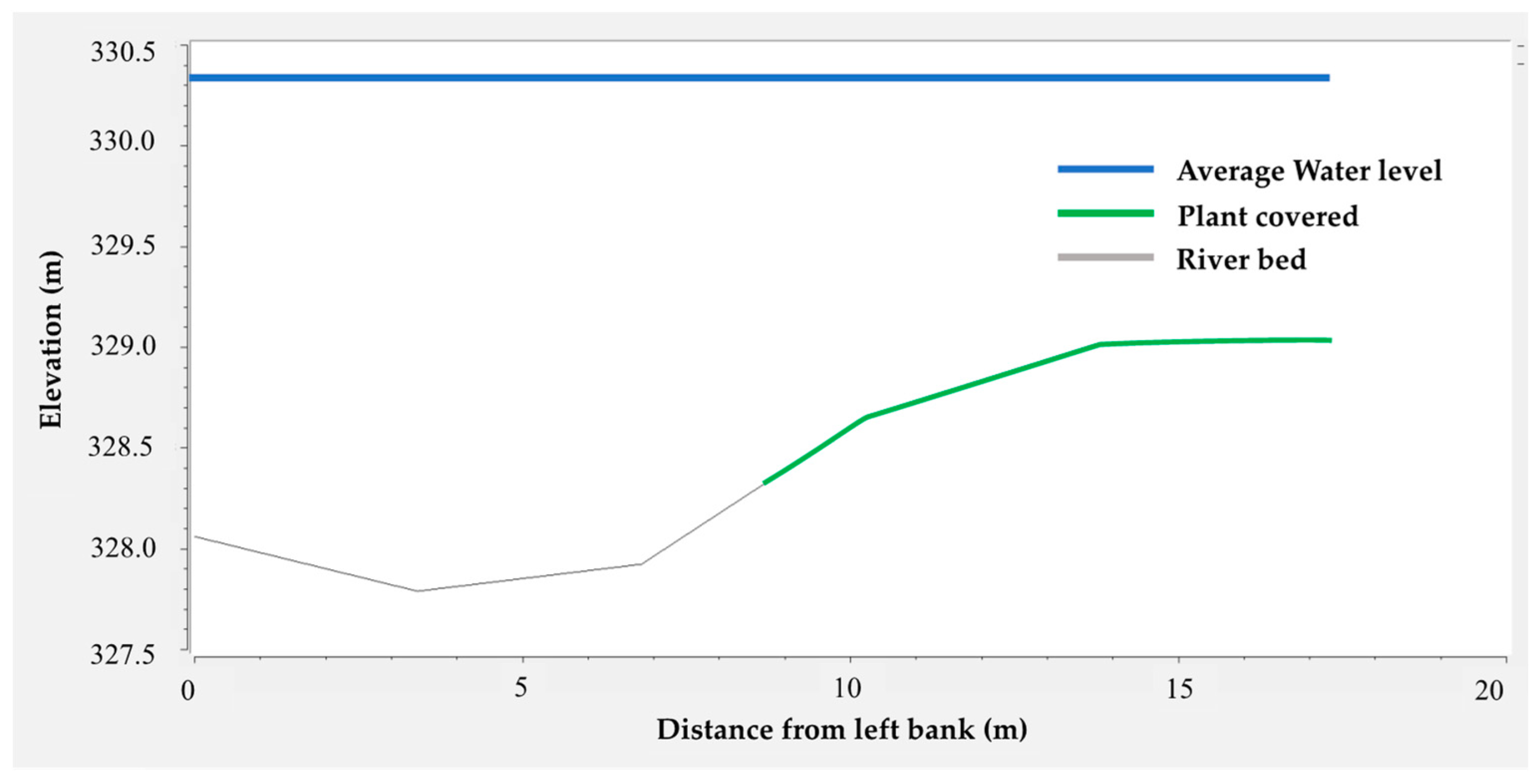
The plants in the channel of the Yamatsuki River are mainly vine reeds covering the sandbars. Many of the crane reeds fell in the downstream direction during the field survey after the river’s outflow. In this analysis, the simulated water depth in the section with the plants was confirmed to be around 1 m (Figure 8). Reeds collapsed at a rate of 0.4 m/s or greater, and the coarse roughness coefficient dropped to around 0.05 [23]. The vital force of the water during flooding likely caused the reeds to collapse, which reduced the roughness coefficient of the plant section and did not have a substantial effect on the Manning’s roughness coefficient.
Because of the collinearity of the physical parameters, the selection of parameters was narrowed down to slope and H/L/S, which have robust correlation coefficients, and a single regression equation with the roughness coefficient was created for each parameter. Figure 9 shows that Manning’s roughness coefficient decreased with an increase in slope, and the trend of an increasing roughness coefficient with increasing H/L/S was very clear. In a previous study, Spearman’s rank correlation coefficient was used to evaluate the influence of slope, watershed area, and size of streambed material on the calculated roughness coefficient [5]. As a result, we confirmed that the slope, bed grain size, and coefficient of roughness were significantly correlated with the riverbed morphology found in gentle gradients, such as plane–bed and pool–riffle gradients, while slope, catchment area, and bed grain size had no effects on roughness in steep gradients, such as step-pool and cascade gradients. However, this study showed that the effects of gradients on roughness coefficients are strong even in channel sections where step pools are observed. In addition, an increase in H/L/S means that the step pool is more developed, and since the loss of flow energy increases as the step pool develops [24,25], an increase in H/L/S is considered to have contributed to the increase in the roughness coefficient. An increase in H/L/S also increases the coefficient of roughness.
To construct an equation to predict the roughness coefficient in mountainous rivers using physical parameters, a multiple regression analysis was conducted with Manning’s roughness coefficient n [m1/3/s] as the objective variable and slope and H/L/S as the explanatory variables featuring high correlation coefficients with the roughness coefficient while taking multi-collinearity into account. As a result, the following regression equation was derived:
n = 0.984777 × S l o p e + 0.012368 × H / L / S + 0.067915 .
The coefficient of determination was 0.60, and the adjusted coefficient of determination was 0.48. Since the coefficient of determination is smaller than 0.5, the accuracy is considered poor. Nevertheless, we believe that these results demonstrate the possibility to create a more accurate prediction equation by increasing the number of samples and conducting similar analyses in the future.

4. Conclusions

This study aimed to collect the spatially and temporally dense water-level data in a mountainous river to back-calculate Manning’s roughness coefficients via a two-dimensional unsteady flow calculation analysis and determine how these coefficients are affected by in-channel physical parameters. The two-dimensional calculation of unsteady flow based on longitudinally observed water levels showed that the roughness coefficient was within the range of the Manning’s roughness coefficient estimated in existing studies. The roughness coefficient calculated by the plane two-dimensional calculations of unsteady flow approached a constant value in the range of 0.05 to 0.1 s/m1/3 as the relative water depth increased. This result indicates that the roughness coefficient can be considered a constant value when performing plane two-dimensional flow calculations for flooding. The roughness coefficient during flooding was found to be correlated with the slope and H/L/S. An equation for predicting the roughness coefficient during flooding based on the physical parameters of the channel was also proposed.

Author Contributions

Conceptualization, T.S. and Y.S.; methodology, H.T., T.S. and S.O.; validation, H.T., S.O. and T.S.; investigation, H.T., S.O. and T.S.; flow calculation, S.O. and T.S.; writing—original draft preparation, H.T.; writing—review and editing, Y.S. and T.S.; supervision, T.S. and Y.S.; project administration, T.S. and Y.S. All authors have read and agreed to the published version of the manuscript.

Funding

This work was supported by JSPS KAKENHI Grant Numbers JP21K04316, JST Grant Number JPMJPF2109 from JAPAN SOCIETY FOR THE PROMOTION OF SCIENCE and the “River Ecology Research Group of Japan” on the Chikugo River from the Ministry of Land, Infrastructure, Transport, and Tourism, Japan.

Data Availability Statement

Date are contained within the article.

Acknowledgments

We wish to thank Taichi Sakabe, Ryota Nakamura, Masaki Oome, and Mizuki Takesue for their field survey assistance and Toshimitsu Kai for providing information on the field.

Conflicts of Interest

Author Shogo Obata was employed by the company Nippon Koei Co., Ltd. The remaining authors declare that the research was conducted in the absence of any commercial or financial relationships that could be construed as a potential conflict of interest.

References

  1. Milliman, J.D.; Syvitski, J.P.M. Geomorphic/Tectonic Control of Sediment Discharge to the Ocean: The Importance of Small Mountainous Rivers. J. Geol. 1992, 100, 525–544. [Google Scholar] [CrossRef]
  2. Reid, L.M. Research and Cumulative Watershed Effects. In General Technical Report; US Department of Agriculture, Forest Service, Pacific Southwest Research Station: Berkeley, CA, USA, 1993; Volume 141, 118p. [Google Scholar] [CrossRef]
  3. Nehlsen, W.; Williams, J.E.; Lichatowich, J.A. Pacific Salmon at the Crossroads: Stocks at Risk from California, Oregon, Idaho, and Washington. Fisheries 1991, 16, 4–21. [Google Scholar] [CrossRef]
  4. Frissell, C.A. Topology of Extinction and Endangerment of Native Fishes in the Pacific Northwest and California (U.S.A.). Conserv. Biol. 1993, 7, 342–354. [Google Scholar] [CrossRef]
  5. Asano, Y.; Uchida, T.; Nishiguchi, Y. Measured Channel Resistance at Mountain Rivers during Flood. Jpn. Soc. Eros. Control Eng. 2018, 70, 12–23. [Google Scholar]
  6. Comiti, F.; Mao, L.; Wilcox, A.; Wohl, E.E.; Lenzi, M.A. Field-Derived Relationships for Flow Velocity and Resistance in High-Gradient Streams. J. Hydrol. 2007, 340, 48–62. [Google Scholar] [CrossRef]
  7. David, G.C.L.; Wohl, E.; Yochum, S.E.; Bledsoe, B.P. Controls on Spatial Variations in Flow Resistance along Steep Mountain Streams. Water Resources Research 2010, 46, W03513. [Google Scholar] [CrossRef]
  8. Reid, D.E.; Hickin, E.J. Flow Resistance in Steep Mountain Streams. Earth Surf. Process. Landf. 2008, 33, 2211–2240. [Google Scholar] [CrossRef]
  9. Rickenmann, D.; Recking, A. Evaluation of Flow Resistance in Gravel-Bed Rivers through a Large Field Data Set. Water Resour. Res. 2011, 47, W0758. [Google Scholar] [CrossRef]
  10. Yochum, S.E.; Comiti, F.; Wohl, E.; David, G.C.L.; Mao, L. Photographic Guidance for Selecting Flow Resistance Coefficients in High-Gradient Channels. In General Technical Report RMRS-GTR; GTR-323; USDA Forest Service: Washington, DC, USA, 2014; pp. 1–91. [Google Scholar]
  11. Marcus, W.A.; Roberts, K.; Harvey, L.; Tackman, G. An Evaluation of Methods for Estimating Manning’s n in Small Mountain Streams. Mt. Res. Dev. 1992, 12, 227–239. [Google Scholar] [CrossRef]
  12. Montgomery, D.R.; Buffington, J.M. Channel-Reach Morphology in Mountain Drainage Basins. Geol. Soc. Am. Bull. 1997, 109, 596–611. [Google Scholar] [CrossRef]
  13. Barnes, H.H., Jr. Roughness Characteristics of Natural Channels. In U.S. Geological Survey Water-Supply Paper; US Government Printing Office: Washington, DC, USA, 1967. [Google Scholar]
  14. Yarahmadi, M.B.; Parsaie, A.; Shafai-Bejestan, M.; Heydari, M.; Badzanchin, M. Estimation of Manning Roughness Coefficient in Alluvial Rivers with Bed Forms Using Soft Computing Models. Water Resour. Manage. 2023, 37, 3563–3584. [Google Scholar] [CrossRef]
  15. Takemura, Y.; Nigo, S.; Ohno, J.; Fukuoka, S. Problem of Conventional 2D Analysis Method for Flood Flows in Mountain Streams with Boulders and Proposal of a New Analysis Method. Adv. River Eng. 2019, 25, 267–272. [Google Scholar]
  16. Liu, Y.; Shimatani, Y.; Yamashita, T.; Sato, T.; Ikematsu, S. Stepped-Bed Morphology Changes in Restoredmountain Stream Inuced by Flood. Adv. River Eng. 2012, 18, 83–88. [Google Scholar]
  17. Shimizu, Y.; Takebayashi, H.; Inoue, T.; Hamaki, M.; Iwasaki, T.; Nabi, M. Nays2DH_SolverManual_Japanese_v4.Pdf. Available online: https://i-ric.org/webadmin/wp-content/uploads/2023/06/Nays2DH_SolverManual_Japanese_v4.pdf (accessed on 1 December 2023).
  18. Ministry of Land, Infrastructure, Transport and Tourism Civil Engineering Work Design Guidelines Part II River Edition Chapter 4 Sabo Facilities. Available online: https://www.qsr.mlit.go.jp/site_files/file/s_top/h22doboku/kasen/2-05.pdf (accessed on 15 December 2023).
  19. Asano, Y.; Uchida, T. Detailed Documentation of Dynamic Changes in Flow Depth and Surface Velocity during a Large Flood in a Steep Mountain Stream. J. Hydrol. 2016, 541, 127–135. [Google Scholar] [CrossRef]
  20. Abrahams, A.D.; Li, G.; Atkinson, J.F. Step-pool Streams: Adjustment to Maximum Flow Resistance. Water Resour. Res. 1995, 31, 2593–2602. [Google Scholar] [CrossRef]
  21. Shawn, M.; Chartrand, P.J.W. Alluvial Architecture in Headwater Streams with Special Emphasis on Step–Pool Topography. Earth Surf. Process. Landf. 2000, 25, 583–600. [Google Scholar]
  22. Hasegawa, K.; Kanbayashi, S. Formation Mechanism of Step-Pool Systems in Steep Rivers and Guide Lines for the Design of Construction. Proc. Hydraulic. Eng. 1996, 40, 893–900. [Google Scholar] [CrossRef]
  23. Fukuoka, S.; Shimatani, Y.; Tamura, H.; Tomari, K.; Nakayama, M.; Takase, A.; Iuch, T. Field Experiments on Reed Deformation and Falling and Roughness Coefficient on Floodchannel by Flows. Adv. River Eng. 2003, 9, 49–54. [Google Scholar]
  24. Ashida, K.; Egashira, S.; Takayuki, N. Structure and friction law of flow over a step-pool bed form. Disaster Prev. Res. Inst. Annu. 1986, 29, 391–403. [Google Scholar]
  25. Wilcox, A.C.; Wohl, E.E.; Comiti, F.; Mao, L. Hydraulics, Morphology, and Energy Dissipation in an Alpine Step-Pool Channel. Water Resour. Res. 2011, 47. [Google Scholar] [CrossRef]
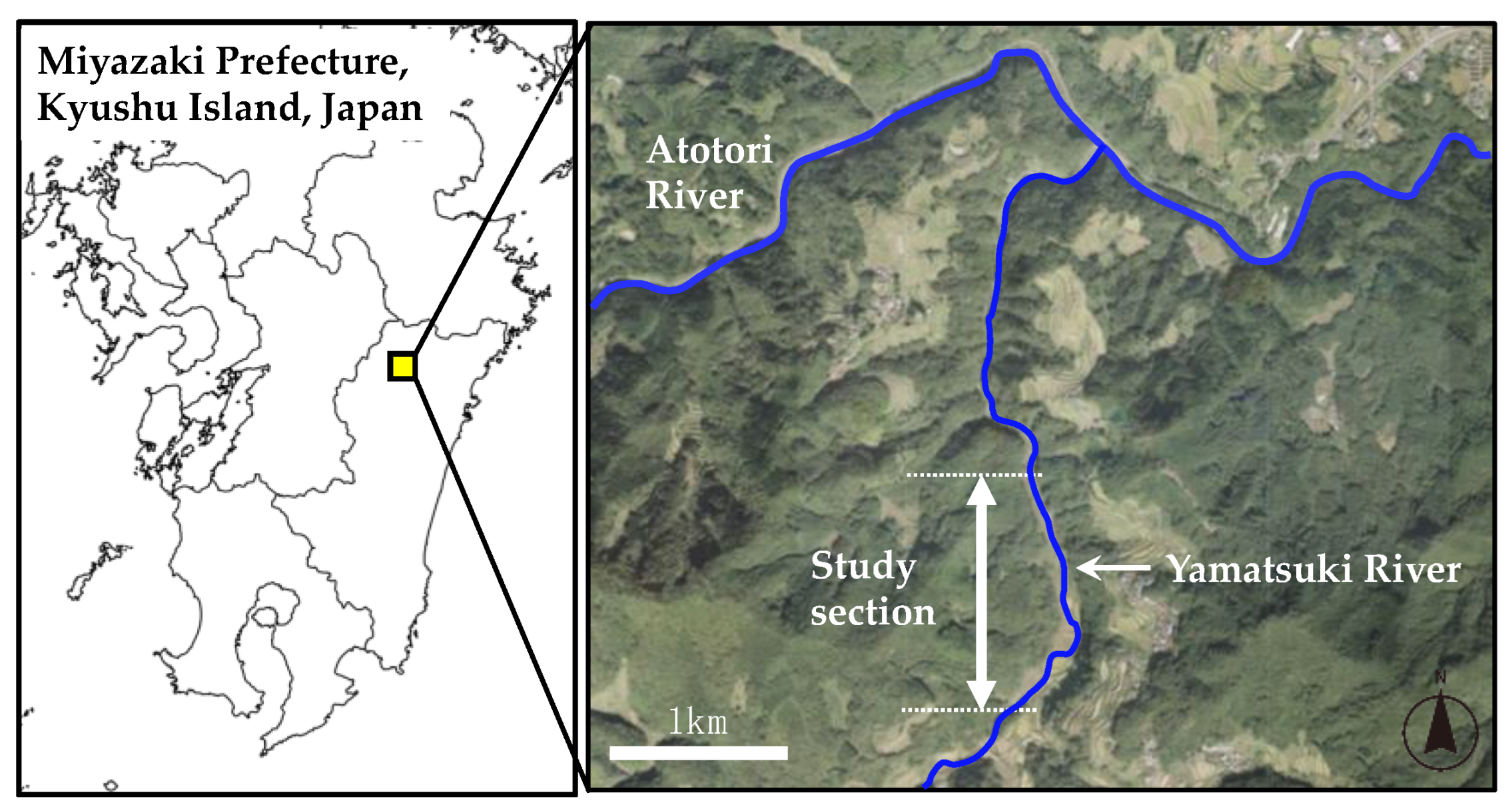
Figure 1. The location of the Yamatsuki River, Miyazaki Prefecture, Kyushu Island, Japan.
Water 16 00320 g001
Figure 2. The river under study: (a) the river during the flood of 2005; (b) the river after the flood of 2005; (c) the river after restoration in 2009.
Water 16 00320 g002
Figure 3. The location of water level gauges in the river and the individual sections in which the Manning’s roughness coefficients were estimated with 2D hydraulic analyses.
Water 16 00320 g003
Figure 4. Hydrograph during the observation period.
Water 16 00320 g004
Figure 5. Relationship between Manning’s roughness coefficient and relative water depth.
Water 16 00320 g005
Figure 6. Longitudinal distribution of back-calculated Manning’s roughness coefficients, calculated water level, and observed water level at peak flow. Calculated water levels in sections 9–11 (WL10), 10–12 (WL11), and 11–13 (WL12) are for reference.
Water 16 00320 g006
Figure 7. Correlation coefficients between measured parameters (red boxes: correlation coefficients exceeding 0.6 for physical parameters that showed a strong correlation with Manning’s roughness coefficient).
Water 16 00320 g007
Figure 8. A cross section at the midpoint of wl08–wl09 with the highest water level.
Water 16 00320 g008
Figure 9. Relationships between Manning’s roughness coefficients, slope, and H/L/S with high correlation coefficients exceeding 0.6.
Water 16 00320 g009
Table 1. Boundary conditions of the ten time periods.
Date and TimeEstimated Discharge at wl04 (m³/s)
8 August 2021 13:000.062
8 August 2021 15:200.416
8 August 2021 17:001.261
8 August 2021 17:201.876
8 August 2021 18:403.611
8 August 2021 19:105.617
8 August 2021 21:006.754
8 August 2021 22:208.056
13 August 2021 7:509.894
13 August 2021 8:2011.519
Table 2. The mean squared error between observed and calculated water levels in each calculation section.
Section NameMean Squared Error
S1–30.00017
S2–40.00031
S3–50.00003
S4–60.00008
S5–80.00023
S6–90.00048
S8–100.00183
S12–140.00012
S13–150.00021
S14–160.00003
Table 3. Data set used in the single and multiple regression analysis.
Cal.
Section
Name
Manning’s Roughness Coefficient (s/m1/3)Ratio of Width to Depth (m/m)Slope
(m/m)
D84
(m)
Relative
Depth
(m/m)
Ratio of Plant
(m2/m2)
Step
(%)
Riffle
(%)
Rapid
(%)
Pool
(%)
H/L/S
S1–30.116.460.0050.402.320.003.0736.872.901.504.02
S2–40.064.940.0251.250.870.003.3822.703.833.041.06
S3–50.066.950.0281.450.610.003.2221.872.226.341.41
S4–60.096.510.0180.551.880.013.7931.390.825.803.11
S5–80.029.000.0350.601.420.227.0816.043.185.772.36
S6–90.0510.290.0350.751.310.395.8420.042.354.712.06
S8–100.0518.230.0400.551.340.634.2424.622.262.321.46
S12–140.109.440.0230.701.840.306.9617.452.028.063.13
S13–150.0711.470.0420.901.080.209.0218.323.184.652.13
S14–160.0712.390.0411.050.760.149.0316.883.957.272.48
Disclaimer/Publisher’s Note: The statements, opinions and data contained in all publications are solely those of the individual author(s) and contributor(s) and not of MDPI and/or the editor(s). MDPI and/or the editor(s) disclaim responsibility for any injury to people or property resulting from any ideas, methods, instructions or products referred to in the content.