Impacts of Climate Change on Ecological Water Use in the Beijing–Tianjin–Hebei Region in China

Abstract

The Beijing–Tianjin–Hebei region in China is experiencing a serious ecological water scarcity problem in the context of climate warming and drying. There is an urgent need for practical adaptation measures to cope with the adverse impacts of climate change and provide a scientific basis for urban water supply planning, water resource management, and policy formulation. Urban ecological water can maintain the structure and function of urban ecosystems, both as an environmental element and as a resource. Current research lacks quantitative analysis of the impact of regional meteorological factors on ecological water use at the small and medium scales. Based on the meteorological data and statistical data of water resources in the Beijing–Tianjin–Hebei (BTH) region, this paper analyzed the trend of climate change and established an ecological climatic water model using gray correlation analysis, polynomial simulation, and singular spectrum analysis to predict the ecological water consumption. And, we assessed the climatic sensitivity of ecological water use and estimated the future ecological climatic water use in the BTH region based on four climate scenarios’ data. The results showed that the average multi-year temperature was 13.2 °C with a clear upward trend from 1991 to 2020 in the BTH region. The multi-year average precipitation was 517.1 mm, with a clear shift in the period of abundance and desiccation. Ecological climatic water modeling showed that a 1 °C increase in temperature will increase ecological water use by 0.73 × 10⁸ m³~1.09 × 10⁸ m³ in the BTH region; for a 100 mm increase in precipitation, ecological water use will decrease by 0.49 × 10⁸ m³~0.88 × 10⁸ m³; under the four climate scenarios of SSP1–2.6, SSP2–4.5, SSP3–7.0, and SSP5–8.5, the regional ecological climatic water use will be 5.14 × 10⁸ m³, 6.64 × 10⁸ m³, 7.82 × 10⁸ m³, and 9.06 × 10⁸ m³ in 2035, respectively; and in 2050, the ecological climatic water use will be 8.16 × 10⁸ m³, 9.75 × 10⁸ m³, 10.71 × 10⁸ m³, and 12.41 × 10⁸ m³, respectively. The methodology and results of this study will support the quantification of climate change impacts on ecological water use in the BTH region and serve as a theoretical basis for future research on ecological water use adaptation to climate change. This study can provide a basis for the development of the overall planning of urban ecological water supply, and at the same time, it can lay a foundation for the study of measures to adapt to climate change by ecological water use.

1. Introduction

The crisis of water shortage is a serious problem in northern China, especially in the Beijing–Tianjin–Hebei (BTH) region. Water has been used to satisfy industrial and agricultural production and urban residents’ livelihoods, resulting in river cutoffs, shrinkage of wetlands, siltation of rivers and streams, and ecological unbalance [1]. Ecological damage, which in turn hinders socio-economic development, has led to a gradual realization of the importance of water ecosystems’ health. The ecological water currently counted includes water supplied by anthropogenic measures to recharge green spaces in towns and cities, some landscaped green spaces and wetlands, and does not include the amount of water naturally met by precipitation and runoff [2].

Ecological water use has been measured since the early 1990s in Beijing and was initially much smaller than other water uses [3]. Since 2003, Tianjin and Hebei have been counting ecological water use [4]. Research on regional ecological water use is growing in abundance [5,6], and Tang et al. [7] summarized several common calculation methods of ecological water use and analyzed the characteristics of vegetation ecological water use. Zhang et al. [8] used Penman’s formula to calculate the changes in the ecological water use of crops and forests in the Heihe River Basin. Zhao et al. [9] calculated the ecological water use of vegetation in the Harbin region using the ecological water use quota method. Wan et al. [10] studied ecological water demand and ecological water supplement in Wuliangsuhai Lake. Wang et al. [11] identified ecohydrological variation in ecosystems and improved the assessment methods for the ecological water demand of valley forests and grasslands in terrestrial ecosystems and for the ecological water level of lake ecosystems in the Irtysh River Basin.

Climate change is an indisputable fact. Continued greenhouse gas emissions will lead to a further increase in global warming, and the global warming among the scenarios and modeled pathways considered will reach 1.5 °C in the near term (2021–2040) [12]. Higher temperatures will accelerate crop transpiration processes, alter crop fertility, and ultimately affect plant water consumption [13]. Changes in the total amount of precipitation, as well as its spatial and temporal distribution, affect the utilization of effective rainfall by plants [14]. Currently, many scholars pay more attention to the impact of climate change on macro water resources’ allocation [15,16]; the impact on ecological water consumption was mostly qualitatively analyzed. Increased temperatures can affect ecological water use by directly affecting evapotranspiration. Reduced precipitation and increased evaporation from the subsurface lead to increased ecological water use. Katri et al. [17] studied the impact of climate change on the ecohydrological environment in southern Finland, and they found that the impacts of climate change can be minimized if ecohydrological modelling methods are used in regional management to reduce the ecological recharge of groundwater. Phayom et al. [18] focused on the impact of climate change on ecohydrological management in northeastern Thailand. It was found that climate change may alter the services provided by ecosystems by changing ecosystem functions. Zhao et al. [19] analyzed the influencing factors of urban ecological water use in Gansu Province based on the combination of AHP-entropy assignment, and the results showed that the green coverage area, the proportion of ecological environmental water use, the per capita park green space area, and the level of urbanization are the main obstacle factors affecting the level of ecological water security, and their contribution is more than 45%, while there is a lack of research on the quantitative impact of regional meteorological factors on ecological water consumption in th BTH region. The urban ecological water consumption selected in this study refers to the partial recharge of water to the green areas and wetlands of urban green parks through artificial measures, which has a certain social nature. At the same time, the impact of climate change should not be ignored: any increase in temperature will accelerate the front transpiration process of plants, change the fertility of plants, and ultimately affect the water consumption of plants; at the same time, the total amount of precipitation in the previous period and the changes in the spatial and temporal distribution of precipitation will also affect the utilization of effective precipitation by plants. Changes in plant water consumption will directly affect ecological water use.

To bridge this gap, here, gray correlation analysis, polynomial simulation, and singular spectrum analysis are proposed to quantitatively analyze the impact of climate change on ecological water consumption and construct a prediction model of ecological climatic water consumption in the context of climate change in the BTH region, in order to provide a theoretical basis for the domestic ecological water use to cope with climate change.

2. Materials and Methods

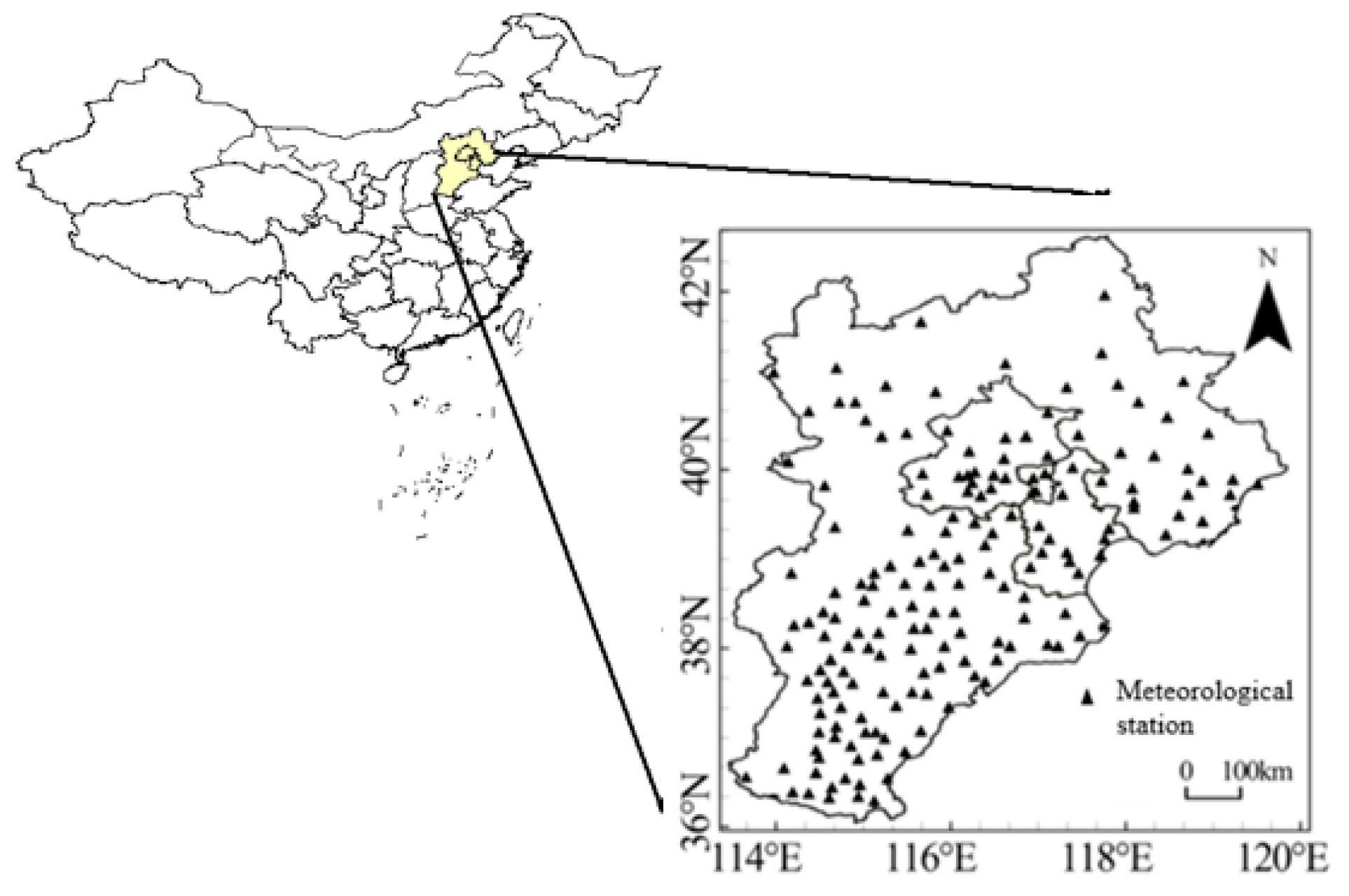
2.1. Data Sources

The Beijing–Tianjin–Hebei region is in China’s North China Plain, between 36°05′ and 42°40′ N and 113°27′ and 119°50′ E. The climate type is a typical temperate continental monsoon climate, rain and heat at the same time, and the annual precipitation is 500–700 mm. In winter, northerly winds prevail, cold and dry, and the average temperature of the coldest month is 0 °C or less; in summer, warm and humid southeasterly winds bring the main precipitation in a year, and the average temperature of the hottest month reaches 20 °C or more. In terms of urban layout, the Beijing–Tianjin–Hebei region, centered on Beijing, Tianjin, and Shijiazhuang, consists of 13 cities with an area of 21.8 × 10⁴ km² and a population of 110 million, accounting for about 8.1 per cent of the country’s total population. The integrated development of Beijing–Tianjin–Hebei is necessary to realize the complementary advantages of Beijing, Tianjin, and Hebei, and drive the development of the northern hinterland. As the capital economic circle, the BTH region is one of the most dynamic economies, the most open, the most innovative, and the most populous region in China. At the same time, it is also one of the regions with the most serious water shortage in China, and the per capita water resources possession is about 1/9 of the national average. One of the major problems facing the sustainable development of the BTH region is the mismatch between the level of economic and social development and the amount of water resources. Therefore, the coordinated development of the Beijing–Tianjin–Hebei region needs to break the administrative restrictions and carry out water resources’ planning and management within the Beijing–Tianjin–Hebei region in unity as a whole. The data used include historical meteorological data, regional water resources data, and future climate scenarios. The historical meteorological data were observed from 171 meteorological stations in the BTH region as shown in Figure 1. The station data from 1991 to 2020 were obtained from the daily-valued dataset of China’s surface climatic data provided by the China Meteorological Administration (for details, please see the China Meteorological Data website at https://data.cma.cn accessed on 18 July 2023), which includes daily temperature and precipitation.

The data on ecological water use in the Beijing–Tianjin–Hebei region are from the Water Resources Bulletin 1991–2020 (for details, please see http://www.mwr.gov.cn/sj/tjgb/szygb/ accessed on 20 July 2023). The socio-economic data came from the Beijing–Tianjin–Hebei Statistical Yearbook 1991–2020, including green coverage rate, urban green space, wetland area, etc.

The Sixth International Coupled Model Comparison Program (CMIP6) was launched to adopt a new scenario with a combination of shared socio-economic pathways and typical concentration pathways. In this paper, the new scenario mainly adopts the four scenarios with four representative future climate scenarios which are SSP1–2.6, SSP2–4.5, SSP3–7.0, and SSP5–8.5, respectively. The future scenario data include maximum temperature, minimum temperature, and precipitation data from the CMIP6 multi-model ensemble of the 20 Global Climate Models (GCMs) (for details, see https://esgf-node.llnl.gov/search/cmip6/ accessed on 16 June 2023). The raw data of the CMIP6 GCMs are on a monthly scale and have a spatial resolution of 1–2°. We used the NWAI-WG statistical downscaling method developed by the Climate Team of the Department of Primary Industries of New South Wales, Australia [20], to downscale the spatial and temporal month-by-month raster data of the various climate models to station data daily. The statistical downscaling method includes three steps:

(1)

Spatial downscaling

The monthly temperature and precipitation data on the raster scale were converted to monthly data on the station scale using the inverse distance weighting (IDW) method, calculated as:

$$s_i={\Sigma }_{k=1}^4\left[\frac{1}{d_{\mathrm{i},k}^m}{\left({\Sigma }_{j=1}^4\frac{1}{d_{\mathrm{i},j}^m}\right)}^{-1}{P}_k\right]$$

(1)

where $s_i$is the predicted value of the pattern of site i after spatial downscaling; $P_k$is the predicted value of the pattern of raster cell k;$d_{i,k}$ is the distance from the center of the site’s raster cell; $m$ is a control parameter, and $m$ is taken as 3 in this paper.

(2)

Bias correction

The climate model data are bias-corrected using station observations and the QQ-mapping bias-correction method to reduce the simulation bias, and the correction equation is:

$$x_k^f=y_i^0+\frac{y_{\mathrm{i}+1}^0-y_i^0}{x_{\mathrm{i}+1}^h-x_i^h}\left(x_k^r-x_i^h\right)x_i^h\le x_k^r\le x_{\mathrm{i}+1}^h$$

(2)

where ($x_k^f\left(k=1,2,\dots ,n\right))$ is the corrected climate model prediction; $x_i^h$ represents the month-by-month data of the model for the assessment period; $x_k^r$ is the pre-correction climate model prediction; and $y_i^0$ represents the month-by-month observation data of the site for the assessment period.

(3)

Temporal downscaling

Daily climate data were generated using the corrected WGEN weather stochastic generator [21] and corrected station-scale monthly climate data. In WGEN, a first-order Markov chain with a gamma distribution is used to model daily precipitation. The probability of rain on a given day depends on the wet or dry state of the previous day. Precipitation is modeled by a two-parameter gamma distribution. The two parameters in the gamma function are alpha and beta, which determine the clarity and scale of the distribution, respectively. The density function of the gamma distribution is given by the following equation:

$$f\left(p\right)=\frac{p^{\alpha -1}{\mathrm{e}}^{\frac{-p}{\beta }}}{{\beta }^{\alpha }\tau \left(\alpha \right)}p,\beta >0,0<\alpha <1$$

(3)

The WGEN parameters for the maximum and minimum temperatures were calculated in a similar manner to precipitation. Serial correlation coefficients were utilized with the number of correlations:

$$X_i\left(j\right)=A{X}_{i-1}\left(j\right)+B{\epsilon }_i\left(j\right)$$

(4)

where $X_i\left(j\right)$ is a matrix containing the three climatic variables (including maximum temperature and minimum temperature) for day i; ${\epsilon }_i$ is an independent random variable; and A and B are matrices defined by the following equation:

$$A=M_1{M}_0^{-1}$$

(5)

$$B{B}^T=M_0-A{M}_1^T$$

(6)

where the elements of $M_0$are the correlation coefficients between the three variables on the same day; the elements of $M_1$ are the correlation coefficients with a lag of 1 day.

Due to the stochastic nature of the downscaling process, the values calculated from the downscaled daily scale data are not always equal to the input monthly values. The downscaled monthly values were evaluated against the monthly values predicted by the GCM through 1500 cycles to ensure that the differences between them were less than the acceptable maximum.

2.2. Methodology

2.2.1. Gray Correlation Analysis

We use gray correlation analysis to analyze the influence of different factors on ecological water use in the BTH region. Gray systems theory considers the prediction of systems that contain both known and unknown or non-deterministic information as the prediction of gray processes that change within a certain orientation and are time dependent. Although the phenomena displayed in the process are random and haphazard, this collection of data has a potential pattern. Gray prediction uses such laws to build gray models and predict a gray system [22,23].

First, the reference series is a time domain of multiple indicators X_0(k) = {X₀₁, X₀₂, X₀₃, ……, X₀}. Xi(k) = {X_i1, X_i2, X_i3, ……, X_in} were the indicator sets of the same length to be evaluated. The next step is to set the dimensionless size of the data. The series is turned into a sequence X_0(k) = {X₀₁, X₀₂, X₀₃, ……, X_0n} and the set of evaluation indicators is normalized as follows: X_ij = {X_i1, X_i2, ……, X_ij, ……, X_in} [24].

The correlation coefficient ξ (X_i) is calculated as follows:

$${\mathsf{\xi }}_{\mathrm{i}}\left(\mathrm{x}\right)=\frac{\underset{\mathrm{i}}{\min }\underset{\mathrm{j}}{\min }|{\mathrm{X}}_{0\mathrm{j}}-{\mathrm{X}}_{\mathrm{ij}}|+\mathsf{\xi }\underset{\mathrm{i}}{\max }\underset{\mathrm{j}}{\max }|{\mathrm{X}}_{0\mathrm{j}}-{\mathrm{X}}_{\mathrm{ij}}|}{|{\mathrm{X}}_{0\mathrm{j}}-{\mathrm{X}}_{\mathrm{ij}}|+\mathsf{\xi }\underset{\mathrm{i}}{\max }\underset{\mathrm{k}}{\max }|{\mathrm{X}}_{0\mathrm{j}}-{\mathrm{X}}_{\mathrm{ij}}|}$$

(7)

The larger the correlation, the stronger the influence of the comparative series on the reference series. It is generally considered that a weak association is 0 < ξ ≤ 0.35; a medium association is 0.35 < ξ ≤ 0.65; a strong association is 0.65 < ξ ≤ 0.85; and a very strong association is 0.85 < ξ ≤ 1.

2.2.2. Singular Spectrum Analysis

Singular spectrum analysis [25,26,27] (SSA) is a typical time-series analysis technique, which introduces various elements of typical time-series analysis, multivariate statistics, multivariate geometry, dynamical systems, signal processing, and singular value decomposition (SVD). It has been widely used in multiple fields such as climate, environment, geography, social science, and finance [28,29], and in many studies on water consumption trend volume extraction introducing singular spectrum analysis [30]. In this paper, singular spectrum analysis was applied to extract the trend terms of ecological water use. The singularity spectrum analysis technique consists of two mutually complementary stages: decomposition and reconstruction.

(1)

Decomposition

Given a real time series $X=\left(x_1,x_2,\dots ,x_{n-1},x_n\right)$of length n, the goal of singularity spectrum analysis is to decompose it into a sum of multiple time series for the purpose of identifying the original series components (e.g., trend, periodic or quasi-periodic, noise, etc.). It can be regarded as a mapping (transformation) operation of the one-dimensional target tensors $X=(x_1,x_2,\dots ,x_{n-1},x_n)$ to the multidimensional affecting tensors $[Z_1,Z_2,\dots ,Z_K]$, $X=\left(x_1,x_2,\dots ,x_{n-1},x_n\right)$→$[Z_1,Z_2,\dots ,Z_K]$, and the result of the mapping operation is the trajectory matrix given the nested dimension:$L\in [2,k]$

$$Z^{*}=\left[\begin{array}{cc}\begin{array}{cc}{x}_1& x_2\\ x_2& x_3\end{array}& \begin{array}{cc}\dots & x_{n-L+1}\\ \dots & x_{n-L+2}\end{array}\\ \begin{array}{cc}⋮& ⋮\\ x_L& x_{L+1}\end{array}& \begin{array}{cc}⋮& ⋮\\ \dots & x_n\end{array}\end{array}\right]$$

(8)

Assume that $S=ZZT$, ${\lambda }_1,{\lambda }_2\dots {\lambda }_L({\lambda }_1\ge {\lambda }_2\ge ,\dots ,\ge {\lambda }_L\ge 0)$ are the eigenvectors of $S$, and the relative eigenvectors standard orthogonalization system is $U_1,U_2,\dots ,U_L$. $d$ is the subscript corresponding to the eigenvalues, and the trajectory matrix $Z^{*}$of the singular value decomposition is expressed as:

$$Z^{*}=Z_1+Z_2+\cdots +Z_d$$

(9)

(2)

Reconstruction

After the expansion of $Z^{*}$ is obtained, the grouping process splits the interval $\left\{1,2,\dots ,d\right\}$ into unconnected subsets $s\left(1\right),s\left(2\right),\dots ,s\left(L\right)$ expanding the time-experiential orthogonal functions (TEOFs), yielding lagged covariances as:

$$S=\left[\begin{array}{cc}\begin{array}{cc}{S}_{\left(1\right)}& S_{\left(2\right)}\\ S_{\left(2\right)}& S_{\left(3\right)}\end{array}& \begin{array}{cc}\dots & S_{\left(L\right)}\\ \dots & S_{\left(L-1\right)}\end{array}\\ \begin{array}{cc}⋮& ⋮\\ S_{\left(L\right)}& S_{\left(L-1\right)}\end{array}& \begin{array}{cc}⋮& ⋮\\ \dots & S_{\left(1\right)}\end{array}\end{array}\right]$$

(10)

The matrix is a square matrix of order L and is called the Toeplitz matrix. It is solved for the eigenvalues of the matrix $S,\left\{{\lambda }_1,{\lambda }_2\dots {\lambda }_k\right\}$ and the corresponding eigen $\left\{E_1,E_2\dots E_k\right\}$, whose full eigenvalues are the singular spectrum of the sequence $x\left(t\right)$.

$$x_{ki}=\left\{\begin{array}{c}\begin{array}{c}{a}_{ik}=\sum _{j=1}^L{x}_{i+1}{E}_{kj}0\le i\le n-L,1\le j\le L\\ \frac{1}{i}\sum _{j=1}^i{a}_{i-\dot{j},k}{E}_{k,j}1\le \mathrm{i}\le L-1\end{array}\\ \frac{1}{L}\sum _{j=1}^L{a}_{i-\dot{j},k}{E}_{k,j}L\le i\le L+1\\ \frac{1}{n-i+1}\sum _{j=i-n+L}^i{a}_{i-\dot{j},k}{E}_{k,j}n-L+2\le i\le n\end{array}\right.$$

(11)

The trend term function:

$${\widehat{x}}_i={\sum }_{k=1}^L{x}_{ki}$$

(12)

2.2.3. Polynomial Simulation Method

Climate change directly and indirectly affects regional ecological water use [31,32], so it is difficult to strip out the impact of climate change from water-use data. Many studies have used polynomial simulation to strip out the effects of meteorological factors on water use [33,34]. In this paper, we use this method to strip the effect of climatic factors on ecological water use in the BTH region, and the changes in urban ecological water use are mainly affected by the green space area, wetland area, green coverage rate, climatic conditions, and other factors, which will be composed of the equation as follows [35]:

$$W_t=W_t^{\prime }+\mathsf{\Delta }{W}_t$$

(13)

where $W_t$ is the actual observed ecological water use; $W_t^{\prime }$ reflects the trend of gradual change in ecological water use, which influenced by factors such as green space area, wetland area, green coverage rate, and was estimated by singular spectrum analysis; $\mathsf{\Delta }{W}_t$ can be interpreted as a perturbation other than the trend change in ecological water use due to climate change such as changes in average annual temperature or precipitation. It was referred to as the climatic water use. Then, the ecological water use was divided into trend terms and climatic water use.

2.2.4. Characterization of Spatial Distribution

The spatial difference of statistical values with latitude and longitude information is performed using the inverse distance weight interpolation (IDW) method in GIS to analyze the spatial changes of statistical values based on the assumption that things that are closer to each other are more similar to each other than those that are farther away from each other.

3. Results

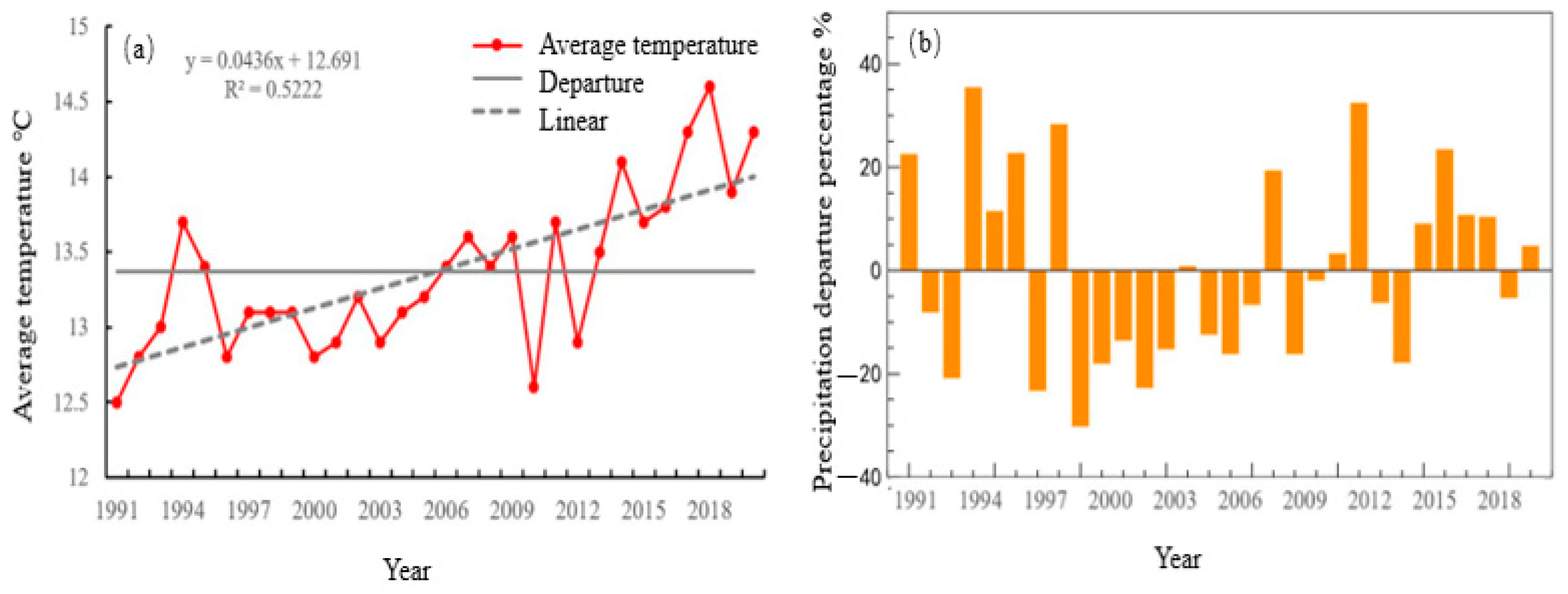
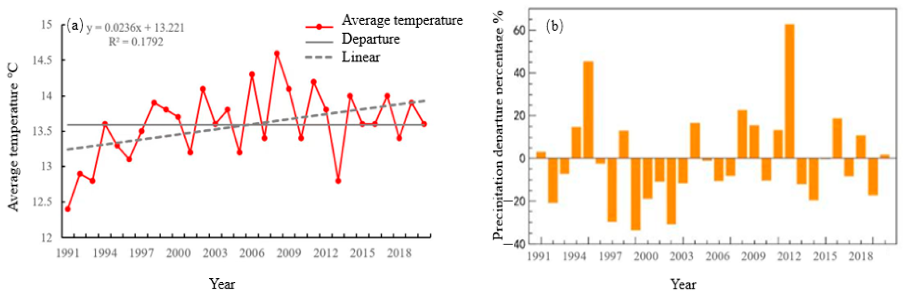
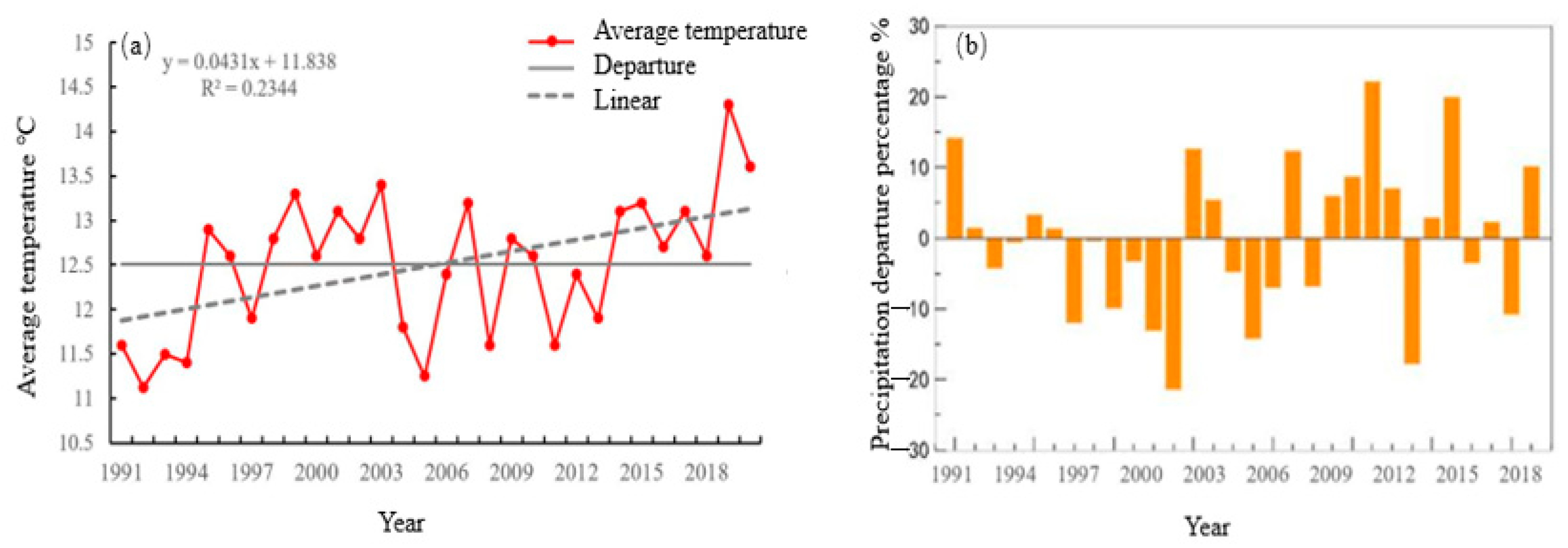
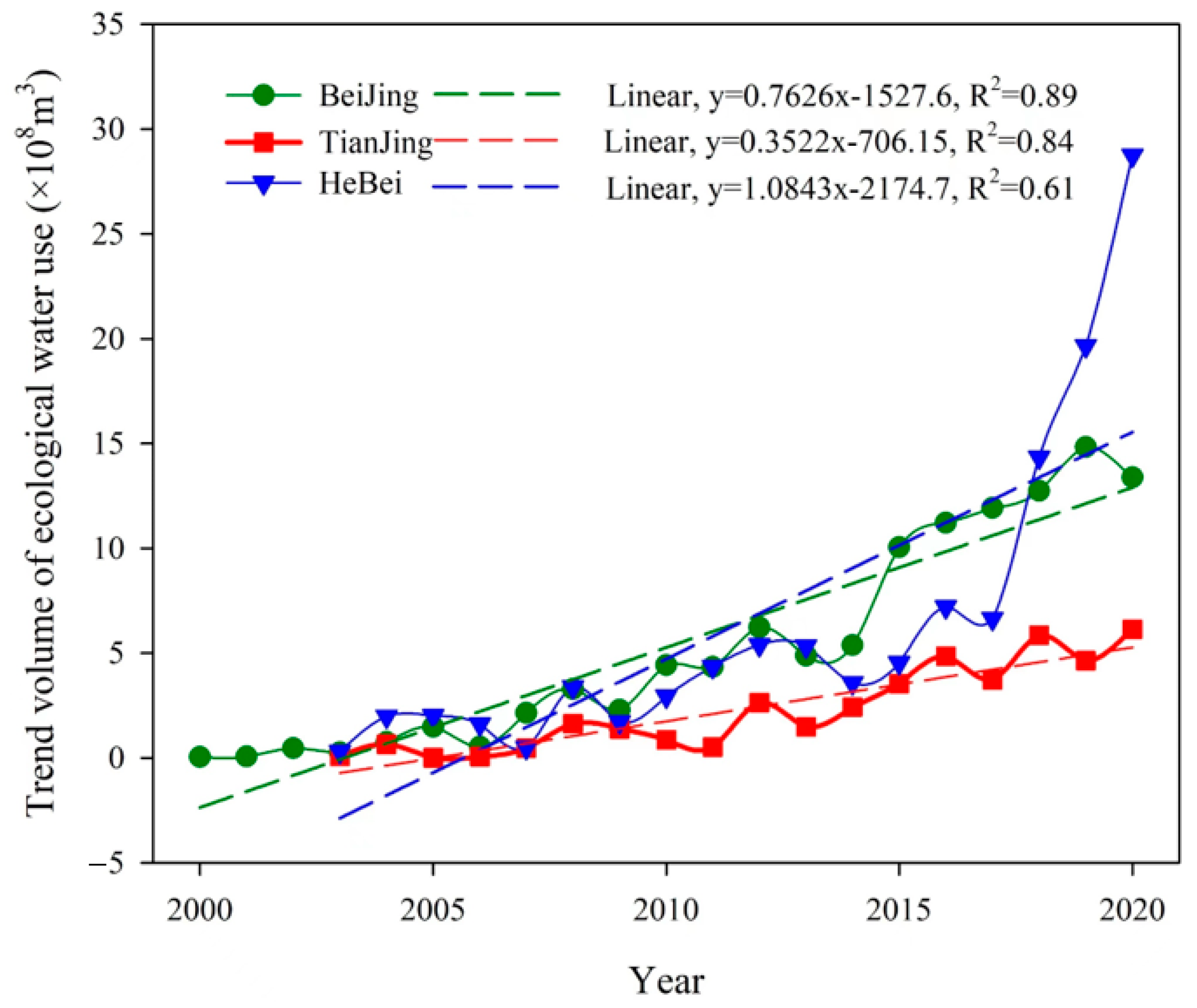
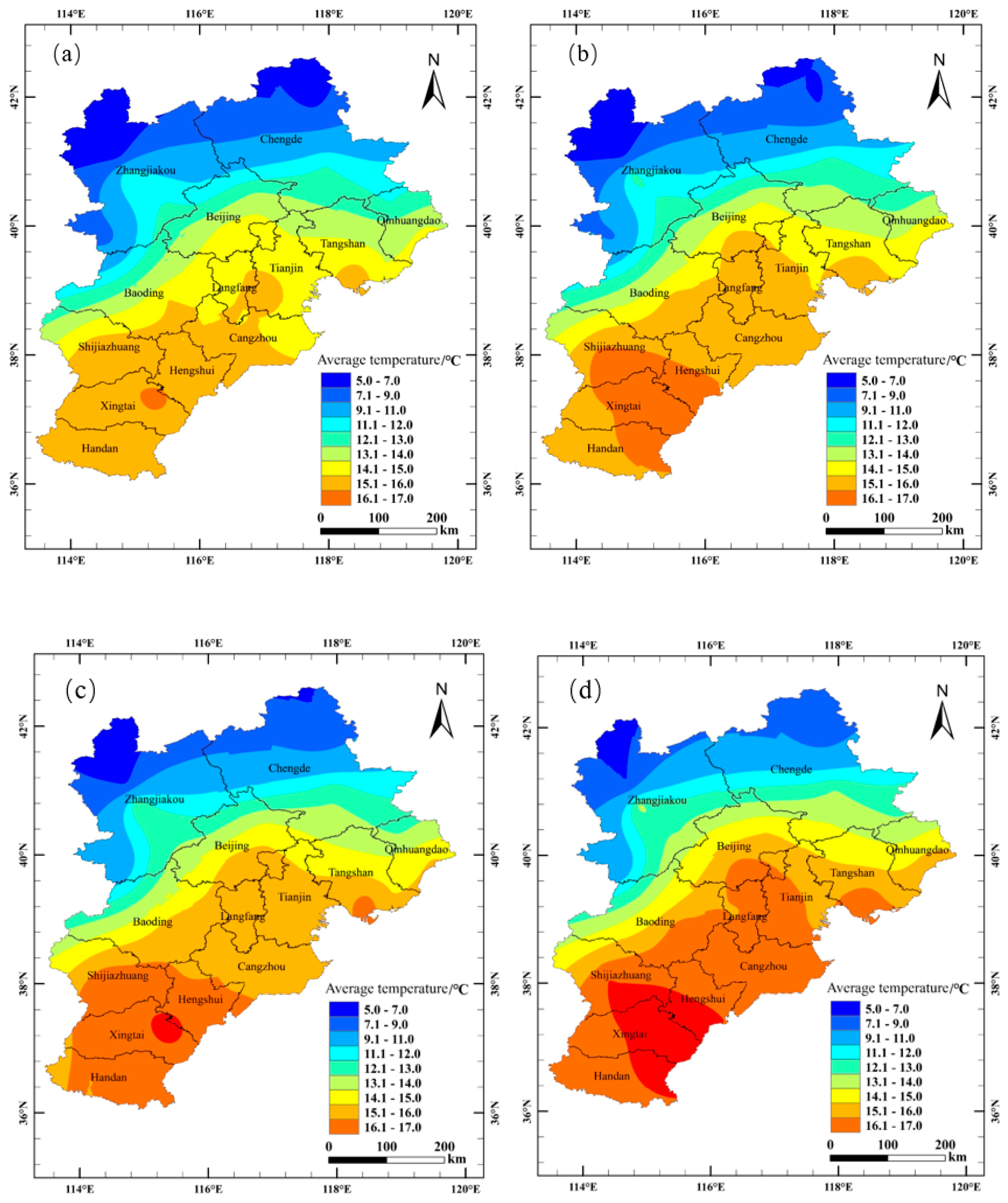
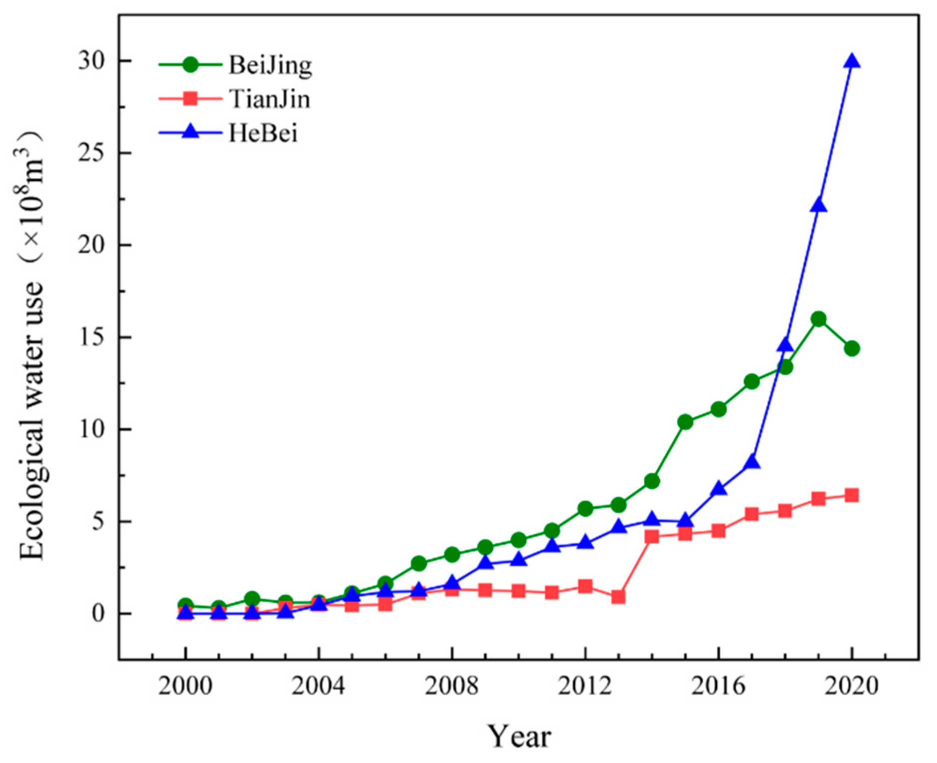
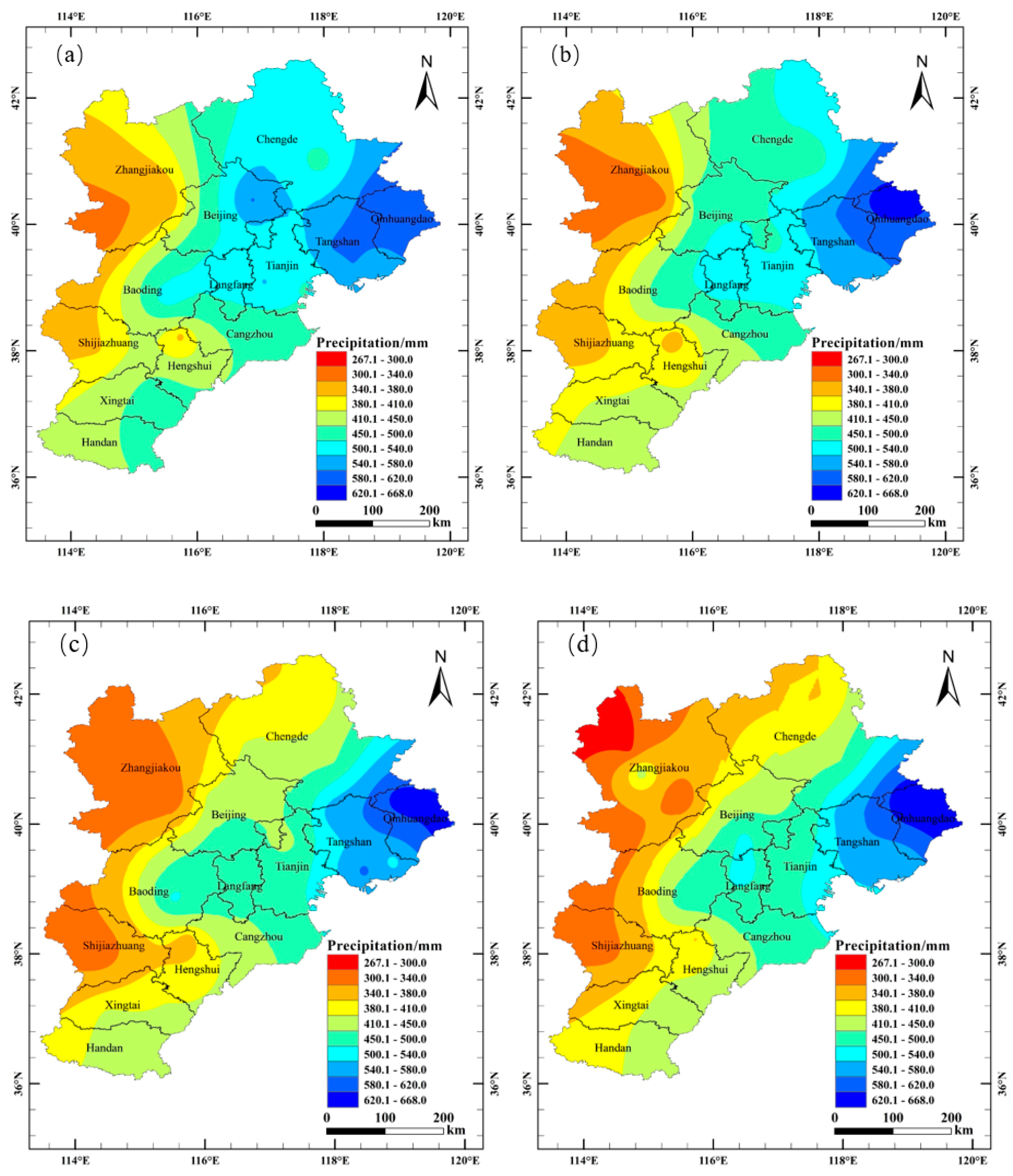
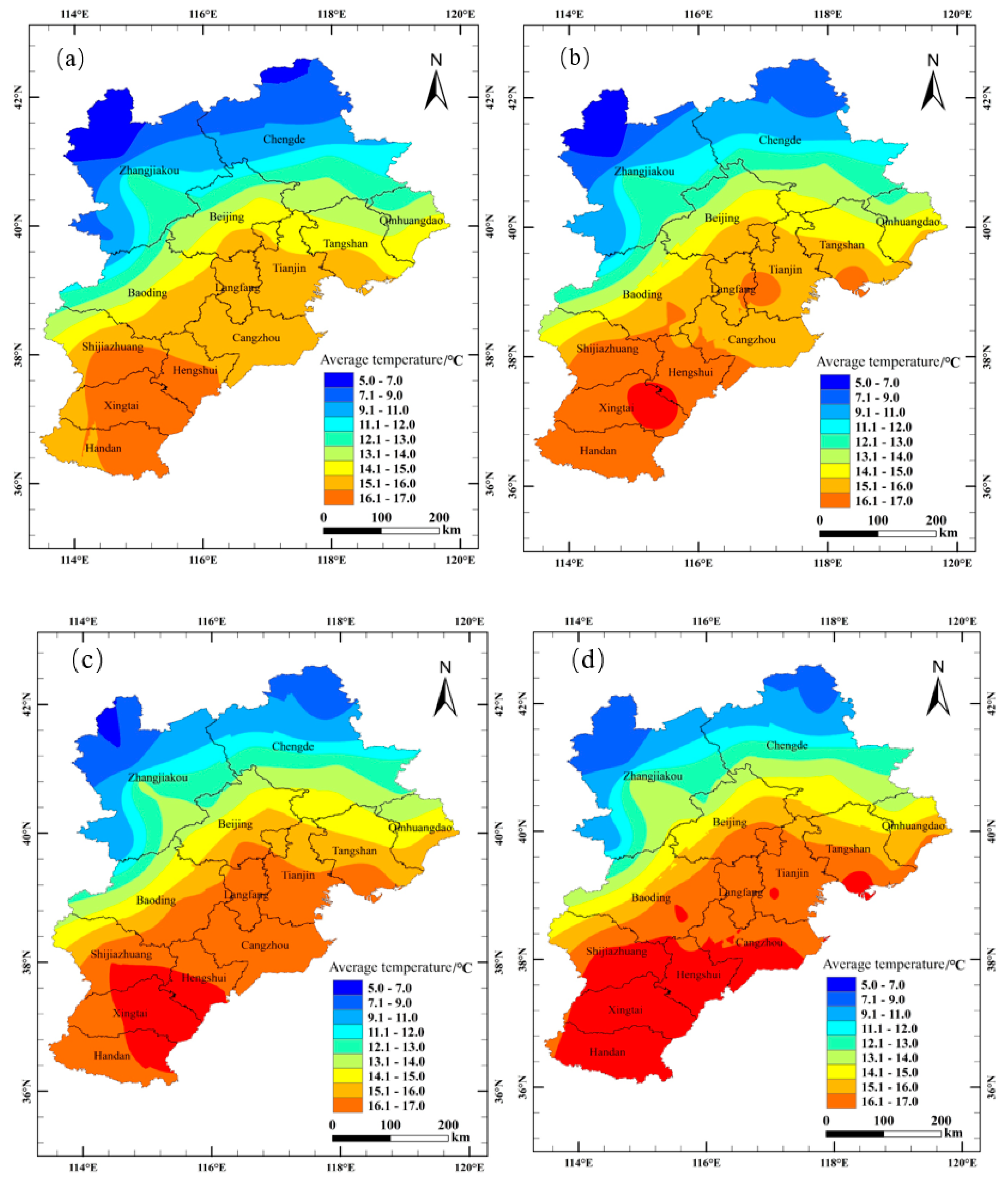
3.1. Characterization of Climate Change and Ecological Water Use in the BTH Region

The interannual variation in the average annual temperature and precipitation in Beijing is shown in Figure 2. The average annual temperature was 13.3 °C from 1991 to 2020 and was rising at a rate of 0.44 °C/10a (p < 0.01). In terms of annual precipitation, the average precipitation was 538.1 mm. The relative variability of precipitation from 1991 to 2020 was 16.27%.

The interannual variation in average temperature and precipitation in Tianjin is shown in Figure 3. The annual average was 13.6 °C from 1991 to 2020 and showed an obvious upward trend in temperature, and the average annual temperature tendency rate was 0.24 °C/10a (p < 0.01). In terms of annual precipitation, the percentage of precipitation fluctuated greatly from 1991 to 2020, and the annual average precipitation was 523.0 mm. There are obvious fluctuations in precipitation and obvious shifts in the abundance and desiccation periods. and the shift of the abundance and depletion period was obvious. The relative variability of precipitation from 1991 to 2020 was 16.3%.

The interannual variation in the average annual temperature and precipitation in Hebei is shown in Figure 4. The average annual temperature was 12.5 °C during 1991–2020, with a significant upward trend, and the temperature tendency rate was 0.43 °C/10a (p < 0.01). In terms of annual precipitation, the fluctuation of the precipitation distance percentage in Hebei was smaller than that in Beijing and Tianjin during 1991–2020, and the average annual precipitation was 496.4 mm. The relative variability of precipitation from 1991 to 2020 was 8.64%.

Since the 21st century, ecological water use has increased in the BTH region, especially after 2004, and the trend of increasing ecological water use has strengthened with the emphasis on environmental protection, as shown in Figure 5, especially in Hebei, from only 0.03 × 10⁸ m³ to 29.92 × 10⁸ m³ from 2000 to 2020, with a growth rate of about 9.87 × 10⁸ m³–10a⁻¹ (p < 0.01).

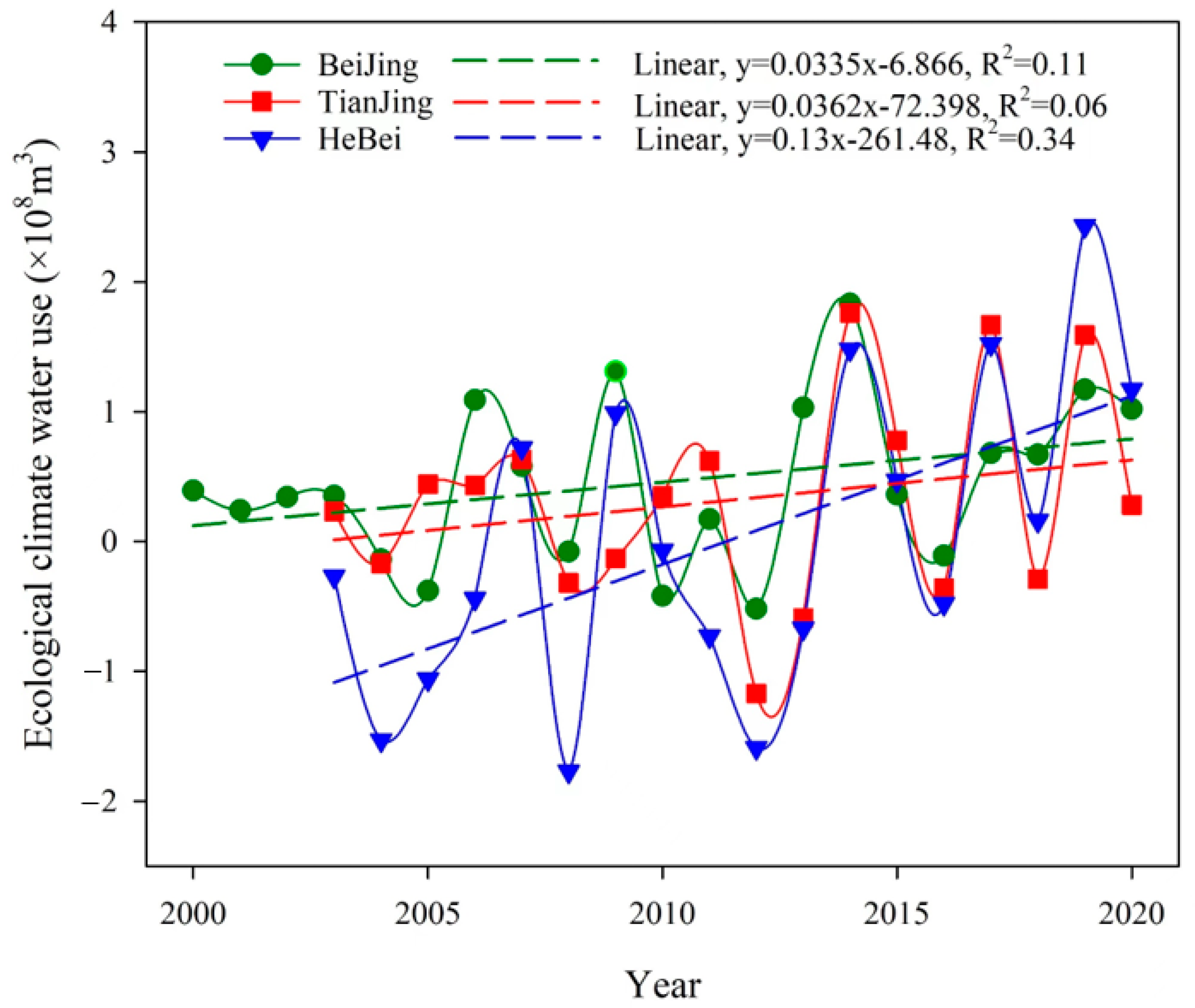
3.2. The Ecological Climatic Water Use in the Beijing–Tianjin–Hebei Region

The ecological water use in the statistics of this study mainly referred to the ecological water use of urban green land and wetland, which was influenced by social and climatic factors. We elected three social influence indicators including the green space area (ha), the wetland area (ha), and green coverage rate (%). The indicators selected for climatic factors included the average annual temperature (°C) and average annual precipitation (mm). Gray correlation was used to analyze the correlation between influencing factors and ecological water use in the BTH region, and the gray correlation coefficients are shown in

Table 1. Gray correlation analysis of ecological water use in the Beijing–Tianjin–Hebei region.

Regions	Average Temperature	Annual Precipitation	Green Space Area	Wetland Area	Green Coverage Rate
Beijing	0.80	0.793	0.967	0.932	0.916
Tianjin	0.771	0.838	0.982	0.973	0.946
Hebei	0.767	0.747	0.995	0.942	0.923

.

Green space area, wetland area, green coverage, and ecological water consumption reached a very strong correlation, indicating that these three factors are the main reasons affecting ecological water use in the BTH region. There was a consistent order for the effect extent on ecological water use among these factors: the green space area had the highest effects, and the green coverage rate had the lowest effects. The average annual temperature and precipitation reached a strong correlation with the ecological water use in the BTH region, indicating that the average annual temperature and precipitation also significantly influenced ecological water use. Overall, the social influence indicators showed a higher effect on ecological water use than those of the climatic indicators.

The method of stripping the meteorological factors on ecological water use is based on polynomial simulation, which divides ecological water use into trend and climatic water use, and for the simulation of the trend term this paper uses singular spectrum analysis. Singular spectrum analysis is based on the general trend of the original series of ecological water use, using the singular spectrum function to fit the water-use series to its impact data series (includes green space area, wetland area, and green coverage rate, and excludes average annual temperature and annual precipitation) and extract the trend term series.

The trend of ecological water use increased significantly with the change in green space area, wetland area, and green coverage rate in the BTH region as shown in Figure 6. Hebei had the highest trend of ecological water use with an average 10.84 × 10⁸ m³/decade, followed by Beijing with the trend of 7.62 × 10⁸ m³/decade, and Tianjin with the trend of 3.52 × 10⁸ m³/decade.

Removing the ecological water-use trend term from the actual ecological water use, we obtained the ecological climatic water use in the BTH region, and its inter-annual variation is shown in the Figure 7. The ecological climatic water use in the BTH region is characterized by fluctuations, with positive values representing the increase in ecological climatic water use caused by climate change and negative values representing the decrease in ecological climatic water use caused by climate change.

3.3. Establishment of Ecological Climatic Water-Use Model in the Beijing–Tianjin–Hebei Region

Finally, we conduct the correlation analysis between the climatic ecological water use and the series of annual average annual temperature and precipitation of the corresponding years, and three ecological climatic water models were established in Beijing, Tianjin, and Hebei, respectively.

The ecological climatic water-use model of Beijing was:

$$y=0.84T-0.0049\mathrm{P}-8.36(R^2=0.71,\mathsf{\alpha }=0.01,p<0.01)$$

(14)

It showed that given a 1 °C increase in the average annual temperature, Beijing’s ecological water use increases by 0.84 × 10⁸ m³, and for a 100 mm increase in precipitation, Beijing’s ecological water use decreases by 0.49 × 10⁸ m³.

The ecological climate water-use model for Tianjin is:

$$y=0.73T-0.0062\mathrm{P}-6.29(R^2=0.66,\mathsf{\alpha }=0.01,p<0.01)$$

(15)

The equation shows that a 1 °C change in the average annual temperature would increase the ecological water use by 0.73 × 10⁸ m³, and a 100 mm increase in precipitation would decrease the ecological water use by 0.62 × 10⁸ m³ in Tianjin.

The ecological climatic water use in Hebei Province was modeled as:

$$y=1.09T-0.0088\mathrm{P}-9.36(R^2=0.85,\mathsf{\alpha }=0.01,p<0.01)$$

(16)

In Hebei, this equation shows that a 1 °C increase in average annual temperature would increase the ecological water use by 1.09 × 10⁸ m³, and a 100 mm increase in precipitation would decrease the ecological water use by 0.88 × 10⁸ m³.

Ecological water use has a consistent positive sensitivity to temperature and a negative sensitivity to precipitation, which indicates that warming would increase ecological water use while wetness would reduce ecological water use. A comparison of the sensitivity of ecological water use to climate change in different regions is given in

Table 2. Comparison table of the sensitivity of ecological water use to climate change in the BTH region.

	Region	Beijing Ecological Climatic Water Use (×108 m3)	Tianjin Ecological Climatic Water Use (×108 m3)	Hebei Ecological Climatic Water Use (×108 m3)
Meteorologic Elements
Average annual temperature rise of 1 °C		0.84	0.73	1.09
Reduction in annual precipitation by 100 mm		0.49	0.62	0.88

. In detail, there were regional differences in the sensitivity of ecological water use to average annual temperature and precipitation: the sensitivity of ecological water use to temperature was stronger in Hebei than in Beijing; the sensitivity of ecological water use to temperature was stronger in Beijing than in Tianjin; and the sensitivity of ecological water use to precipitation in Hebei was stronger than that in Tianjin and Beijing.

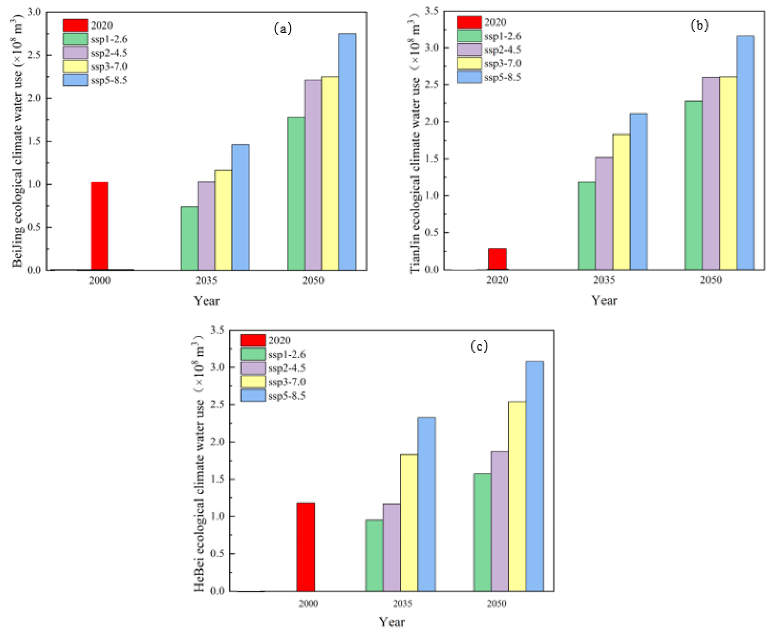
3.4. Projections of Ecological Climatic Water Use in the Beijing–Tianjin–Hebei Region under Future Scenarios

The spatial distribution of average temperature and annual precipitation in the Beijing–Tianjin–Hebei region under future scenarios is plotted by spatially interpolating the statistical values with latitude and longitude information using the inverse distance weight interpolation (IDW) method in GIS. In 2035, the spatial distribution of the average temperature exhibits a trend of gradual decrease from the south to the north under the four different scenarios (Figure 8). With increased radiation force, the trend of increasing temperature in the southern part of the BTH region is obvious. The average annual temperatures in Beijing are 13.8 °C, 14.1 °C, 14.2 °C, and 14.6 °C, respectively. The average annual temperatures under the four scenarios in Tianjin are 14.7 °C, 15.3 °C, 15.4 °C, and 15.7 °C, respectively. The average annual temperatures in Hebei Province under the four scenarios are 13.4 °C, 13.5 °C, 13.9 °C, and 14.4 °C.

The distributions of annual precipitation under the four different scenarios are shown in Figure 9. The spatial distribution of precipitation shows a decreasing trend from east to west. The annual precipitation in Beijing under the four scenarios is 509.3 mm, 501.8 mm, 491.8 mm, and 499.7 mm, which is lower than the average of 538.1 mm during 1990–2020. The average annual precipitation in Tianjin under the four scenarios is 524.6 mm, 541.2 mm, 503.4 mm, and 493.7 mm, respectively, and the precipitation of the SSP126 and SPP2–4.5 scenarios is higher than the average annual precipitation during 1990–2020, which is 523.0 mm, while the average annual precipitation under the SSP3–7.0 and SSP5–8.5 scenarios is lower than the average annual precipitation during 1990–2020. The precipitation in Hebei Province under the four scenarios is 488.5 mm, 475.2 mm, 450.1 mm, and 455.4 mm, respectively, which is lower than the annual precipitation of 496.4 mm from 1990 to 2020.

In 2050, there is a significant warming compared to that in 2035, with a decreasing trend from south to north as shown in Figure 10. With increased radiative forcing of the four scenarios, the temperature tends to increase significantly, and the average annual temperatures in Beijing are 14.7 °C, 15.2 °C, 15.3 °C, and 15.8 °C, respectively. The average annual temperatures in Tianjin under the four scenarios are 15.6 °C, 16.1 °C, 16.2 °C, and 16.7 °C, respectively. The average annual temperatures in Hebei are 13.9 °C, 14.1 °C, 14.5 °C, and 15.0 °C, respectively.

The distribution of annual precipitation shows a decreasing trend from east to west, and there is a significant decrease in precipitation in the western part of the region compared with that of 2035 (Figure 11). The annual precipitation in Beijing under the four scenarios is 449.8 mm, 449.1 mm, 457.7 mm, and 441.7 mm, which is lower than the average of the precipitation during 1991–2020 (538.1 mm). The annual precipitation in Tianjin is 454.4 mm, 460.8 mm, 471.3 mm, and 452.4 mm, which is lower than the average precipitation of 523.0 mm in Tianjin during 1991–2020. The precipitation in Hebei is 479.7 mm, 470.3 mm, 444.1 mm, and 444.5 mm, respectively.

Based on the temperature and precipitation of the future scenarios in the BTH region and the modeling of the ecological climate water use, the ecological climate water use for the four scenarios in 2035 and 2050 is predicted (Figure 12). With the enhancement of radiative forcing, the ecological climatic water use in the BTH area has significantly increased. Tianjin’s ecological climatic water use is higher than that of 2020 under all four scenarios. Under the SSP1–2.6 scenario, the ecological climate water use in Beijing and Hebei Provinces can be well controlled. The ecological climatic water use in 2035 for the SSP5–8.5 scenario is 1.46 × 10⁸ m³ in the Beijing region, 2.11 × 10⁸ m³ in the Tianjin region, and 2.33 × 10⁸ m³ in the Hebei region. By 2050, the ecological climate water use in the SSP5–8.5 scenario will be 2.75 × 10⁸ m³ in Beijing, 3.16 × 10⁸ m³ in Tianjin, and 3.08 × 10⁸ m³ in Hebei.

4. Discussion

Over the past 30 years, the average annual temperature in the BTH region has presented a significantly increasing trend, which is consistent with the studies by Xu et al. [36]. Precipitation in the BTH region has obvious volatility, and the shift of the abundance and waning period is obvious, which is consistent with the results of Lu et al. [37]. The main factors of ecological water consumption in the BTH region are green space area, wetland area, and green coverage rate, but the impact of climate warming on ecological water consumption should not be ignored. Higher temperatures affect the transpiration of vegetation in the BTH region, leading to an increase in water consumption by vegetation and an increase in ecological water use in the region; the higher the precipitation, the less artificial recharge required, leading to a decrease in ecological water use. Zhang et al. [38] estimated the ecological water use in the Haoxi watershed under the background of climate change and found that the average annual ecological water use increased by 0.27 billion m³, 0.21 billion m³, and 0.29 billion m³ from 2025 to 2100 under the scenarios of RCP2.6, RCP4.5, and RCP8.5, respectively. Wang et al. [39] pointed out that the temperature change has an impact on the evapotranspiration of vegetation, which affects the regional ecological water use, and precipitation affects the water replenishment of the ecosystem. This study gives a method for how to quantitatively analyze the impact of climate change on ecological water use in the BTH region and estimates ecological and climatic water use under different scenarios in the future, which provides a reference for the macroscopic allocation of water resources in the Beijing–Tianjin–Hebei region and is conducive to the precise allocation of the South-to-North Water Diversion Project. On the one hand, we need to scientifically grasp the relationship between agricultural water, industrial water, domestic water, and ecological water use in water resources’ planning to fully reflect the multi-purpose water resources, multi-functional scientific treatment of industrial and agricultural production of water, domestic water, and ecological water use of water, so that they all provide their respective benefits. From the perspective of the sustainable utilization of water resources, water conservation is the basis and the main means to ensure ecological water use, and the fundamental method is to improve the efficiency of water resources’ utilization, and apply the saved water resources to the ecological water use so as to ensure the ecological environment of the Beijing–Tianjin–Hebei region. On the other hand, for the increase in ecological water consumption caused by climate change, the government should look for new ways to develop water resources, such as urban and rural sewage treatment, seawater desalination, and so on. At the same time, water, energy, and food are interrelated, constrained, and dependent on each other. They are important factors affecting economic growth and social stability. At the present stage, there are potential risks associated with a single-resource management approach, and the conclusions of this study are favorable to the development of a multi-system study. The conclusions of this study are conducive to the development of multi-system studies to strengthen intersectoral synergies and cooperation and to support the safe development of the coupled system of water, energy, and food.

In this paper, the limitations of this study are that when establishing the ecological and climatic water consumption model, we only used temperature and precipitation as the main climatic indicators. But some studies have shown that wind speed and solar radiation also have a certain impact on ecological water consumption [40]. In future, more meteorological factors should be included in the selection of indicators for climate factors. Ecological water use is both a resource and an environmental element. The ecological climate water-use trend prediction model developed in this paper and the combination of CMIP6 multi-model climate change scenario data to predict the ecological climate water use in the BTH region in 2035 and 2050 under different scenarios can provide a basis for urban water supply planning and water management and provide a climatological basis for the government and different sectors to formulate water-conservation measures. With increased ecological water consumption due to climate change, government departments should look for new ways to develop water resources, such as urban and rural wastewater treatment and seawater desalination. However, further research is needed to find the most suitable adaptation paths to climate change for ecological water use in the BTH region.

5. Conclusions

This paper analyzes the meteorological factors affecting ecological water use, establishes a prediction model for ecological water use, and reveals the impacts of climate change on ecological water use in the BTH region under different climate scenarios. It is found that the average annual temperature in the BTH region is 13.2 °C for many years, with an obvious upward trend, in which the average temperature tendency rate is 0.436 °C/10a in Beijing, 0.236 °C/10a in Tianjin, and 0.431 °C/10a in Hebei. The precipitation in the BTH region has obvious abundance and depletion, and the average precipitation for many years is 517.1. This paper establishes an eco-climate water-use trend prediction model and finds that for every 1 °C increase in the average annual temperature, the ecological water use in the BTH region increases by 0.73 × 10⁸ m³ ~ 1.09 × 10⁸ m³; for every 100 mm increase in precipitation, the regional ecological water use decreases by 0.49 × 10⁸ m³ ~ 0.88 × 10⁸ m³. However, this model only predicts the effect of average annual temperature and precipitation on ecological water use and does not capture the effect of other meteorological factors such as wind speed and solar radiation on ecological water use. Combined with the data from the CMIP6 multi-model climate change scenarios, the SSP1–2.6, SSP2–4.5, SSP3 SSP1–2.6, SSP2–4.5, SSP3–7.0, and SSP5–8.5 scenarios, the ecological and climatic water use in the BTH region in 2035 is 5.14 × 10⁸ m³, 6.64 × 10⁸ m³, 7.82 × 10⁸ m³, and 9.06 × 10⁸ m³, respectively; and in 2050, the ecological and climatic water use in the BTH region is 8.16 × 10⁸ m³, 9.75 × 10⁸ m³, 10.71 × 10⁸ m³, and 12.41 × 10⁸ m³, respectively. 10⁸ m³ and 12.41 × 10⁸ m³, respectively. These findings are very important for urban water supply planning and water management. The methodology presented in this paper can help water resource managers in water-scarce cities in China to estimate future ecological water demand in the context of environmental change. Reliable estimates of future water demand can assist in planning for the sustainable management of water resources. The study could serve as a perfect example to support decision making on water use and climate change adaptation-related issues.

References

1. Li, Y.; Liu, T. Reconstruction of the Beijing-Tianjin-Hebei eco-environmental governance system and coordinated development idea. Huanjing Baohu Kexue 2023, 49, 52–57. [Google Scholar]
2. Zhang, Z.; Yang, Z.; Yang, M. Analysis and trend prediction of ecological environment water related factors in Beijing, Tianjin and Hebei. Haihe Water Resour. 2018, 1, 4–6+25. [Google Scholar]
3. Ji, L.; Li, J. Characterization of domestic water consumption of residents in urban areas of Beijing, Tianjin and Hebei. Green Sci. Technol. 2022, 24, 122–127. [Google Scholar]
4. Zhen, N.; Rutherfurd, I.; Webber, M. Ecological water, a new focus of China’s water management. Sci. Total Environ. 2023, 879, 163001. [Google Scholar] [CrossRef]
5. Nan, T.; Cao, W. Effect of Ecological Water Supplement on Groundwater Restoration in the Yongding River Based on Multi-Model Linkage. Water 2023, 15, 374. [Google Scholar] [CrossRef]
6. Sun, Q.; Zhang, C.; Yuan, J.; Dong, J.; Xia, L.; Zhou, Y. Characteristics and Problem Analysis of Water Supply and Demand for Urban Environments in Arid and Water-deficient Regions of North China, Using the Taiyuan Urban Area as an Example. Terr. Ecosyst. Conserv. 2022, 2, 29–38. [Google Scholar]
7. Tang, Z.; Ma, X.; Sheng, L. Estimation of Ecological Water Consumption and Vegetation Ecological Construction. Huanjing Baohu 2004, 9, 1–33. [Google Scholar]
8. Zhang, J.; Li, D. Analysis on variations of ecological water demand in growth periods in Heihe valley. Agric. Res. Arid Areas 2006, 24, 164–168. [Google Scholar]
9. Zhao, X. Research on Ecological Water Demand and Rational Allocation of Water Resources in Harbin City. Master’s Thesis, Harbin Institute of Technology, Harbin, China, 2012. [Google Scholar]
10. Wan, F.; Zhang, F.; Zheng, X.; Xiao, L. Study on Ecological Water Demand and Ecological Water Supplement in Wuliangsuhai Lake. Water 2022, 14, 1262. [Google Scholar] [CrossRef]
11. Wang, D.; Zhang, S.; Wang, G.; Gu, J.; Wang, H.; Chen, X. Ecohydrological Variation and Multi-Objective Ecological Water Demand of the Irtysh River Basin. Water 2022, 14, 2876. [Google Scholar] [CrossRef]
12. Fan, X.; Qin, Y.; Gao, X. Interpretation of the main conclusions and suggestions of IPCC AR6 Working GroupⅠReport. Huanjing Baohu 2021, 49, 44–48. [Google Scholar]
13. Wang, Z.; Sun, C.; Liu, Y.; Jiang, Q.; Zhu, T. Spatiotemporal variation of vegetation index and its response to climate factors in Heilongjiang Province. Nanshui Beidiao Yu Shuili Keji 2022, 20, 737–747. [Google Scholar]
14. Hua, S.; Cai, X.; Yu, X. Study on the Evapotranspiration Features of Vegetation Over Flat Underlying Surface and Response to Meteorological Factors. J. Soil Water Conserv. 2016, 30, 344–350+354. [Google Scholar]
15. Yang, L.; Feng, Q.; Zhu, M.; Wang, L.; Alizadeh, M.R.; Adamowski, J.F.; Wen, X.; Yin, Z. Variation in actual evapotranspiration and its ties to climate change and vegetation dynamics in northwest China. J. Hydrol. 2022, 607, 127533. [Google Scholar] [CrossRef]
16. King, D.A.; Bachelet, D.M.; Symstad, A.J.; Ferschweiler, K.; Hobbins, M. Estimation of potential evapotranspiration from extraterrestrial radiation, air temperature and humidity to assess future climate change effects on the vegetation of the Northern Great Plains, USA. Ecol. Modell. 2015, 297, 86–97. [Google Scholar] [CrossRef]
17. Rankinen, K.; Holmberg, M.; Peltoniemi, M.; Akujärvi, A.; Anttila, K.; Manninen, T.; Markkanen, T. Framework to Study the Effects of Climate Change on Vulnerability of Ecosystems and Societies: Case Study of Nitrates in Drinking Water in Southern Finland. Water 2021, 13, 472. [Google Scholar] [CrossRef]
18. Saraphirom, P.; Wirojanagud, W.; Srisuk, K. Potential Impact of Climate Change on Area Affected by Waterlogging and Saline Groundwater and Ecohydrology Management in Northeast Thailand. EnvironmentAsia 2013, 6, 19–28. [Google Scholar]
19. Zhao, B.; Huang, J.; Li, Z.; Li, J.; Zhou, Y. Comprehensive Evaluation and Influencing Factor Analysis of Urban Ecological Water Security in Gansu Province Based on AHP-Entropy Method. Bull. Soil Water Conserv. 2023, 43, 167–173+213. [Google Scholar]
20. Liu, D.; Zuo, H. Statistical downscaling of daily climate variables for climate change impact assessment over New South Wales, Australia. Clim. Change 2012, 115, 629–666. [Google Scholar] [CrossRef]
21. Richardson, C.W.; Wright, D.A. WGEN: A Model for Generating Daily Weather Variables; Computer Science, Agricultural and Food Sciences, Environmental Science; United States Department of Agriculture, Agricultural Research Services: Washington, DC, USA, 1984.
22. Hu, Y.; Cai, G.; Xu, X.; Zhang, M. Empirical Study on Driving Forces of Construction Land Expansion in Wuhan City Based on Grey Relational Analysis. Bull. Soil Water Conserv. 2014, 34, 214–218. [Google Scholar]
23. Huang, X.; Huang, D. Statistical Characteristics of Guangxi Agricultural Meteorological Disaster Situation and Grey Relation Analysis. J. Meteorol. Res. Appl. 2014, 35, 67–70+90. [Google Scholar]
24. Zhang, D. Grey Correlation Analysis between Meteorological Factors and Regional Air Pollution Concentration. Environ. Sci. Manag. 2019, 44, 79–83. [Google Scholar]
25. Lu, W.; Wen, Y. Singular Spectrum Analysis on the Climatic Characteristics of Minle County during 1968–2007. Anhui Nongye Kexue 2011, 39, 16831–16832+16928. [Google Scholar]
26. Krishnan, C.; Mahesha, A. Assessment of Bi-Decadal Groundwater Fluctuations in a Coastal Region Using Innovative Trends and Singular Spectrum Analysis. J. Geol. Soc. India 2023, 99, 111–119. [Google Scholar] [CrossRef]
27. Zhao, L.; Liu, Y. Singular Spectrum Analysis on Carbon Dioxide Emissions of Energy Consumption in Beijing Municipality and Shanghai Municipality. Sci. Technol. Manag. Res. 2015, 35, 236–244. [Google Scholar]
28. Zhu, W.; Dou, H.; Yin, N.; Cheng, Y.; Zhang, S.; Zhang, Q. Deformation characteristics analysis of the expansive soil slope by integrating of InSAR and SSA techniques: A case study of the South-to-North Water Diversion Project. Cehui Xuebao 2022, 51, 2083–2092. [Google Scholar]
29. Hudson, L.I.; Keatley, R.M. Singular Spectrum Analytic (SSA) Decomposition and Reconstruction of Flowering: Signatures of Climatic Impacts. Environ. Model. Assess. 2017, 22, 37–52. [Google Scholar] [CrossRef]
30. Xiao, S.; Wang, G.; Tu, Y. The SSA+FBPF Method and Its Application on Extracting the Periodic Term from BeiDou Satellite Clock Bais. Cehui Xuebao 2017, 45, 172–178. [Google Scholar]
31. Du, X.; Zhao, X.; Wang, H.; He, B. Responses of terrestrial ecosystem water use efficiency to climate change: A review. Shengtai Xuebao 2018, 38, 8296–8305. [Google Scholar]
32. Lei, Y. Impact of Climate Change on Ecological Environment and Ecological Water Requirement in the Yellow River Basin. Water Conserv. Sci. Technol. Econ. 2018, 24, 31–37. [Google Scholar]
33. Dou, Y. Economic Growth and Climate Change Impact on Domestic Water Changes and Grey Correlation Analysis in Urumqi City. Water Conserv. Sci. Technol. Econ. 2015, 21, 1–3. [Google Scholar]
34. Wu, H.; Long, B.; Pan, Z.; Lun, F.; Song, Y.; Wang, J.; Zhang, Z.; Gu, H.; Men, J. Response of Domestic Water in Beijing to Climate Change. Water 2022, 14, 1487. [Google Scholar] [CrossRef]
35. Wei, J.; Chen, Z.; Peng, Y. Correlation Analysis on Daily Water Supply and Meteorological Factors in Wuhan City. Meteorol. Mon. 2000, 26, 27–29+51. [Google Scholar]
36. Xu, C.; Lu, C.; Wang, J. Characteristics of climate change in Beijing-Tianjin-Hebei region in recent 60 years. Water Resour. Hydropower Eng. 2021, 52, 12–20. [Google Scholar]
37. Lu, D.; Yan, L.; Xu, X.; Li, J.; Xu, D.; Yao, R. Analysis of Extreme Precipitation Trend in Beijing-Tianjin-Hebei Region Based on Various Trend Analysis Methods. Renmin Huanghe 2022, 44, 26–32. [Google Scholar]
38. Zhang, Y.; Kang, W.; Qiao, H.; Long, Y.; Zhang, C. Estimated ecological water demand in the context of climate change—Take the Haoxi River Basin as an example. Nanshui Beidiao Yu Shuili Keji 2023, 21, 313–323. [Google Scholar]
39. Wang, Y.; Yang, W.; Xing, B.; Luo, Y. A study of influencing factors of spatio-temporal evapotranspiration variation across the Yellow River Basin under the Budyko framework. Shuiwen Dizhi Gongcheng Dizhi 2023, 50, 23–33. [Google Scholar]
40. Chao, T.; Lin, L.C.; Ting, T.Y. Impacts of anthropogenic and biophysical factors on ecological land using logistic regression and random forest: A case study in Mentougou District, Beijing, China. J. Mt. Sci. 2022, 19, 433–445. [Google Scholar]
Figure 1. Distribution of the meteorological stations in the study area.
Water 16 00319 g001
Figure 2. Trend of temperature (a) and precipitation (b) in Beijing.
Water 16 00319 g002
Figure 3. Trend of temperature (a) and precipitation (b) in Tianjin.
Water 16 00319 g003
Figure 4. Trend of temperature (a) and precipitation (b) in Hebei.
Water 16 00319 g004
Figure 5. Interannual trends of ecological water use in the Beijing–Tianjin–Hebei region.
Water 16 00319 g005
Figure 6. Trend of ecological water use in the Beijing–Tianjin–Hebei region. Note: Tianjin and Hebei started counting ecological water use in 2003.
Water 16 00319 g006
Figure 7. Ecological climatic water use in the Beijing–Tianjin–Hebei region. Note: Tianjin and Hebei started counting ecological water use in 2003.
Water 16 00319 g007
Figure 8. Distribution of average annual temperature in the Beijing–Tianjin–Hebei region under different scenarios in 2035. Note: (a) the temperature under the SSP1–2.6 scenario, (b) the temperature under the SSP2–4.5 scenario, (c) the temperature under the SSP3–7.0 scenario, and (d) the temperature under the SSP5–8.5 scenario.
Water 16 00319 g008
Figure 9. Precipitation distribution under different scenarios in the Beijing–Tianjin–Hebei region in 2035. Note: (a) the precipitation under theSSP1–2.6 scenario, (b) the precipitation under the SSP2–4.5 scenario, (c) the precipitation under the SSP 3–7.0 scenario, and (d) the precipitation i under the SSP5–8.5 scenario.
Water 16 00319 g009
Figure 10. Distribution of average annual temperature in the Beijing–Tianjin–Hebei region under different scenarios in 2050. Note: (a) the temperatures under the SSP1–2.6 scenario, (b) the temperatures under the SSP2–4.5 scenario, (c) the temperatures under the SSP3–7.0 scenario, (d) the temperatures under the SSP5–8.5 scenario.
Water 16 00319 g010
Figure 11. Precipitation distribution under different scenarios in the Beijing–Tianjin–Hebei region in 2050. Note: (a) the precipitation under the SSP1–2.6 scenario, (b) the precipitation under the SSP2–4.5 scenario, (c) the precipitation under the SSP3–7.0 scenario, and (d) the precipitation under the SSP5–8.5 scenario.
Water 16 00319 g011
Figure 12. Ecological climate water use in the Beijing–Tianjin–Hebei region for future scenarios. Note: (a) Beijing, (b) Tianjin, (c) Hebei.
Water 16 00319 g012