Assessing the Effectiveness of Alternative Tile Intakes on Agricultural Hillslopes

Abstract

Existing surface inlets behind terraces and water and sediment control basins (WASCoBs) were replaced with alternative tile intakes (ATIs) in agricultural fields of southeast Iowa. These ATIs consisted of a buried column of gravel atop woodchips. Computational, experimental, and field methods were used to design and evaluate the ATIs’ capacity to reduce sediment and nutrient export. Single-storm simulations using the Watershed Erosion Prediction Project (WEPP) provided boundary conditions for permeameter experiments that yielded a hydraulic conductivity for the layered gravel–woodchip configuration of 4.59 cm/s ± 0.36 cm/s. Additionally, a proportional amount of sediment was retained in the permeameter (42%) compared to the amount that settled on the permeameter surface (58%). Event monitoring of field-installed ATIs during three growing seasons measured a sediment trapping efficiency of 86 ± 12% that led to deposition rates of 5.44 ± 3.77 cm/yr, quantified with ²¹⁰Pb profiles. Percent reduction values were 43% for nitrate and 17% for ortho-phosphate. Finally, long-term continuous-storm modeling using the WEPP suggested that these ATIs could withstand at least 75 25-year events before clogging. Modeling using the Agricultural Conservation Planning Framework suggested watershed-scale load reductions of 1.6% for NO₃ and 1.4% for total P for ATIs draining 6.8% of the modeled watershed. Using ATIs in conjunction with WASCOBs and terraces, or as standalone practices, can be a cost-effective means for keeping sediment and nutrients in the landscape.

1. Introduction

Excessive erosion has always been an unfortunate consequence of agriculture: see, e.g., [1]. To curb soil loss, structural practices like terraces or water and sediment control basins (WASCoBs) can be implemented along agricultural hillslopes. These earthen-mound structures are placed in series subdividing the slope length of a field. They force runoff to ponds, allowing some sediment to settle. The water eventually drains through a surface inlet to a buried conduit.

The surface inlets typically consist of orange slotted pipes extending up from the ground. These slotted pipes drain excess water from a field, as well as enhance sediment settling. They have a reported sediment trapping efficiency of up to 66%, as seen in, e.g., [2]. However, the intakes have little capacity to trap finer sediment sizes or remove dissolved nutrients from the runoff. The drain tiles subsequently convey and export the fine sediment and nutrients directly to the receiving stream.

Tile drainage has altered hydrologic and ecological regimes in the U.S. Midwest [3]. It has increased baseflow, modified recession characteristics, and homogenized hydrologic responses, as seen in, e.g., [4]. The tile discharge is also a major source of nitrate-nitrogen [5,6] and dissolved phosphorus [7,8,9] for waterways draining agricultural watersheds. Reducing excess sediment and nutrient discharge from tiles has become a major component of several states’ nutrient reduction strategies: see, e.g., [10].

For this study, slotted inlets were replaced with less-obtrusive alternative tile intakes (ATIs). These ATIs (Figure 1) consist of a buried column of gravel augmented with an underlying layer of woodchips. Sediment trapping is primarily achieved through enhanced settling from runoff ponding around the intake. A secondary trapping mechanism is performed through filtration before the runoff passes into the drain tile.

An ATI is projected to be more efficient than a traditional inlet at removing finer sediment and sorbed nutrients from runoff. Gravel intakes have been shown to trap 80–98% of the delivered sediment and sediment-bound constituents, like phosphorus. This is an improvement over the observed 66% for orange slotted pipes [2]. ATIs are also designed to increase the effective hydraulic retention time of the nutrient-laden runoff to optimize the potential for denitrification. The added woodchip layer stimulates denitrification to remove fertilizer-derived NO₃. The sizes of the arrows in Figure 1 decrease progressing through the figure, which represents the ATI slowing runoff flux, allowing more time for denitrification to occur.

ATIs are still novel. In fact, only a few states have considered them, such as in, e.g., [11,12,13]. Currently, there is very little available information regarding flow and sediment dynamics within gravel intakes used in agricultural systems, let alone the ATI design presented in this study [14].

The goal of this study is to provide insight into the performance of these modified structures for limiting losses of sediment and associated nutrients from agricultural fields. It demonstrates the utility of ATIs through computational, experimental, and field means that characterize the key parameters of hydraulic conductivity, which represents the flow-through capacity of the ATI, and trapping efficiency, which describes the functional usefulness of the ATI. In addition, appendices are included describing the installation process of an ATI, which can be in conjunction with WASCOBs/terraces or by itself, as well as the ATI costs and economic benefits. This detailed study is the first to showcase these ATIs and their capacity to retain sediment and nutrients, thus preserving productivity.

2. Materials and Methods

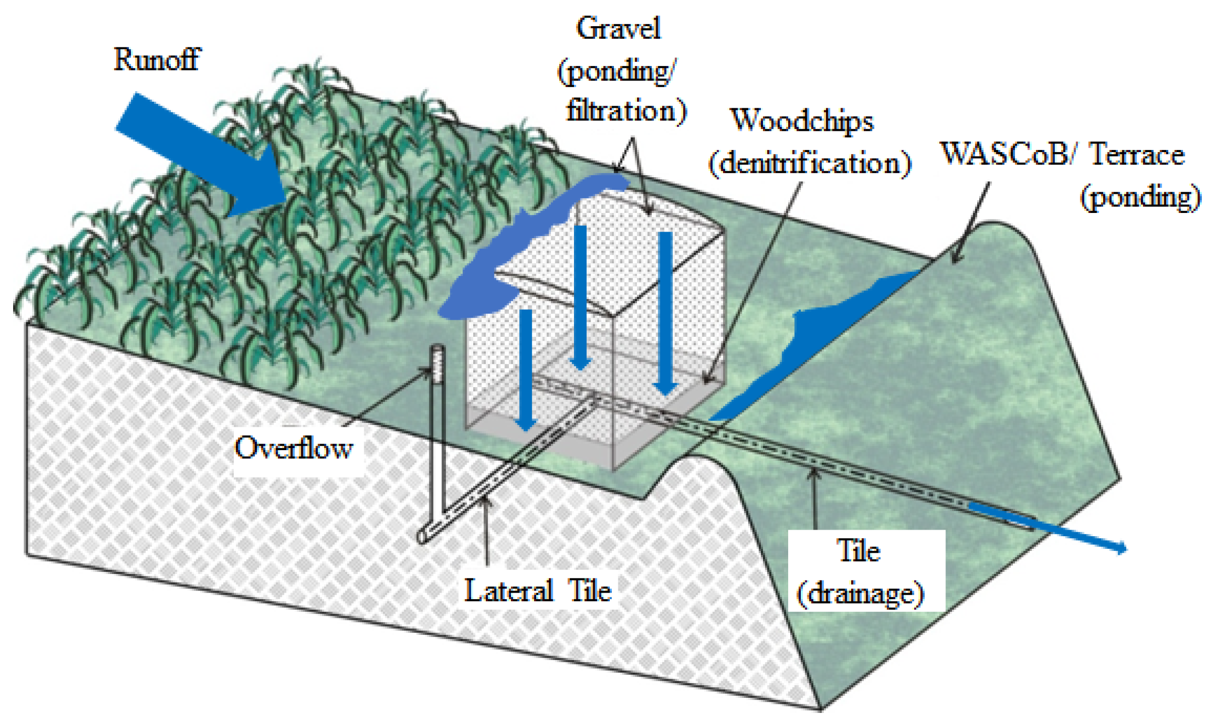
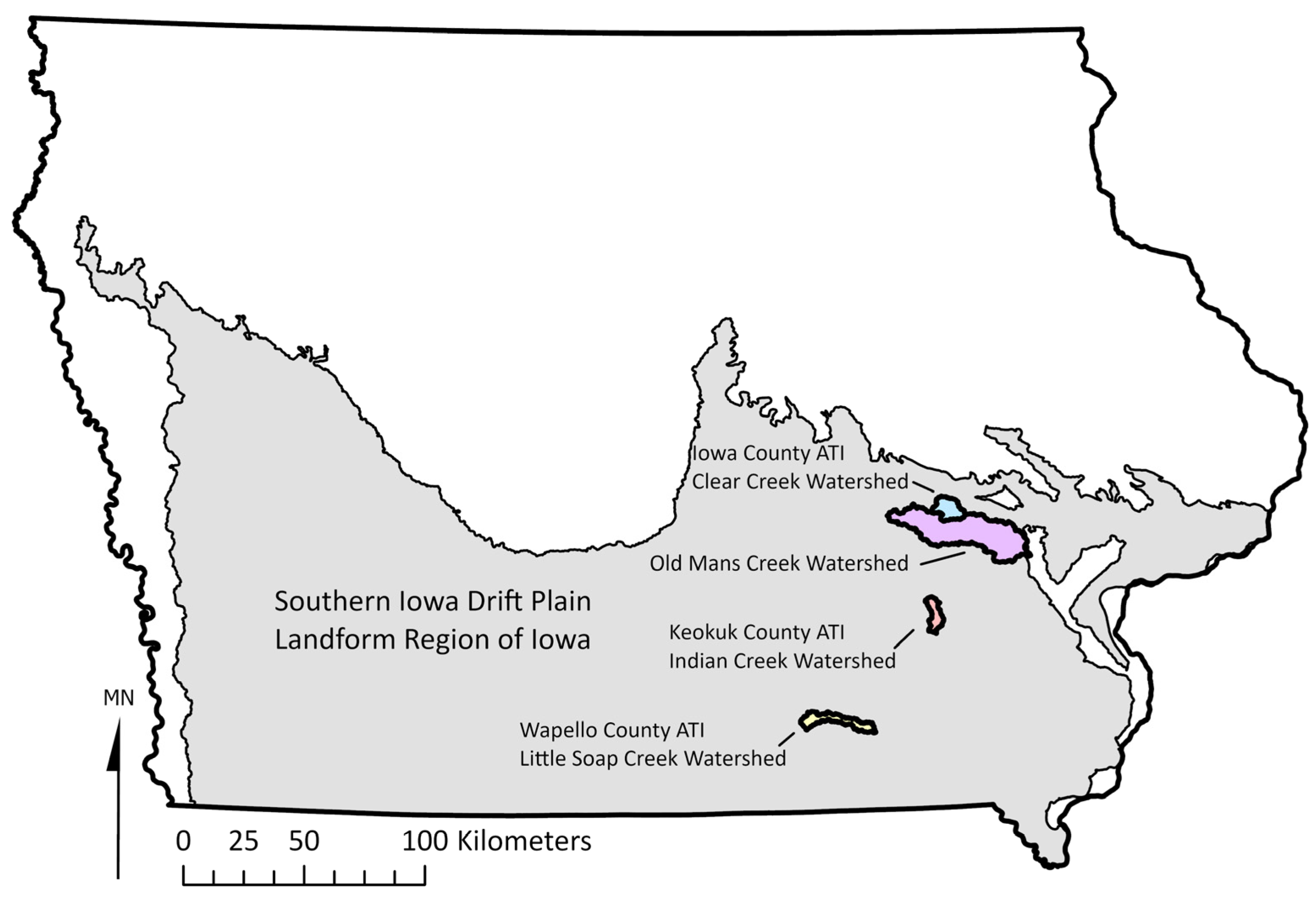
2.1. Study Site

This study occurred in the Southern Iowa Drift Plain region of the U.S. Midwest (Figure 2). This region consists of rolling landscapes with thinning Wisconsin-age loess (from 3 to 10 m deep) and post-settlement alluvium overlying pre-Illinoian till [15]. The silty loam (SL) and silty clay loam (SCL) soils have well-developed, organic-rich surface horizons that are slowly permeable [16]. The predominant upland soil series are Tama (SL), Fayette (SL), and Otley (SCL). The lowlands contain the Colo (SCL), Nodaway (SL), and Zook (SL) series. Silt contents are >65%, with clay contents between 24% and 32%. Organic matter contents are 3% to 4%. Saturated hydraulic conductivity values are between 0.0001 and 0.0005 cm/s. The average annual precipitation for this region during the study period was approximately 900 mm and the average annual temperature was 10 °C [17]. This region is also predominately under row crop agriculture. Thus, the landscape has been re-shaped by rain events and overland sediment movement, enhanced through agricultural tillage [18].

Three ATIs were established in southeast Iowa (Figure 2) for monitoring their effectiveness at reducing sediment and nutrient exports from intensively managed agricultural fields. More specifically, the ATIs were in the following watersheds: Clear Creek in Iowa County; Indian Creek in Keokuk County; and Little Soap Creek in Wapello County.

At the Iowa County site, the existing surface inlets upslope of three WASCoBs were replaced with ATIs (Figure 3a). The primary ATI, which was monitored during this study, was installed in June 2011 and drains 0.24 ha of an upland farm under a 2-year reduced-till corn/no-till soybean rotation. The remaining ATIs were installed in December 2011.

The Keokuk County ATI was installed in March 2019 in a field under a traditional corn/soybean rotation that incorporates cereal rye cover crops. It replaced a surface tile inlet associated with a grass-backed WASCoB. This ATI is similar in size to those in Iowa County, and it drains 0.65 ha. The tile drainage system here originates at the inlet, and there are no lateral tile lines.

The ATI in Wapello County was also installed in March 2019. It is behind a farmable contour terrace in a field under a traditional corn/soybean rotation. This ATI is similar in size and material make-up to the other ATIs and drains 1.38 ha. At the Wapello site, the drainage system also originates at its inlet and there are no lateral tile lines.

These ATIs (Figure 3b) were all sized similarly following the procedure outlined in this article’s Appendix A. The overall dimensions of each ATI were 2.44 m (l) × 0.61 m (w) × 1.22 m (d). The ATIs extended in depth to the existing drain tile. Drain tiles in the study area consisted of 10–15 cm diameter, slotted, corrugated plastic pipes, typically installed 1.22 m below the soil surface. The excavated soil pit over the drain tile was lined with non-woven Class III geotextile. The hardwood chips (D₅₀ = 0.51 cm) were laid first in the excavated pit. Approximately 0.45 m³ of woodchips was applied evenly to a depth of 0.30 m. Then, ~1.36 m³ of washed pea gravel (D₅₀ = 1.03 cm) was applied to a depth 0.9 m. The porosity of the system was 0.43. Further details of the ATI design are in [14].

2.2. Method Overview

A combination of computational, experimental, and field methods was used in this study to design and evaluate the performance of ATIs in reducing the export of sediment and nutrients from agricultural fields. Initially, single-storm simulations were conducted using the Watershed Erosion Prediction Project, or the WEPP, to establish boundary conditions for permeameter experiments. The permeameter experiments were used to characterize, under controlled conditions, the parameters of hydraulic conductivity and trapping efficiency. Building from these experiments, ATIs installed along three hillslopes in southeast Iowa were monitored during the growing seasons of 2013, 2019, and 2021 for their delivery of and ability to flow through sediment, nitrogen, and phosphorus. Finally, additional modeling determined the expected lifespan of the ATIs through continuous-storm simulations using the WEPP and extrapolated their performance to the watershed scale using the Agricultural Conservation Planning Framework (ACPF) toolbox.

2.3. Modeling

2.3.1. Water Erosion Prediction Project (WEPP)

The WEPP has been used extensively in Iowa and the U.S. Midwest: e.g., in [19,20]. Detailed descriptions of the model’s parameterization, calibration, and validation for fields in southeast Iowa are in [21,22].

The WEPP is a physically based, distributed-parameter, runoff-and-erosion model that considers heterogeneity in soil, land use, and topographic parameters along a hillslope. The hydrologic component in the WEPP first calculates infiltration rates and then runoff rates using the continuity equation and overland flow routing. Hence, the WEPP can be more accurate than approaches relying on the Rational method, curve numbers, and site-specific runoff information [23]. The model has an added extension for DRAINMOD that calculates tile flow [24]. Regarding the modeling of sediment movement on hillslopes with the WEPP, soil erosion begins with interrill erosion. Soil particles detach through raindrop impact and are delivered to the rills. The detachment, transport, and deposition of sediment in the rills are then calculated using a steady-state solution to the 1D sediment continuity equation [25]. It provides net erosion rates based on these mechanistic approaches. In addition, the WEPP comes with a complete management practice database.

The weather data from National Weather Service sites in Williamsburg, Sigourney, and Ottumwa were obtained through the Iowa MESONET web site [17]. These are the closest monitoring sites to the installed ATIs (<10 km). A lengthy period (since 1960) was used to ensure the model processes were at a steady state before simulating the monitoring period. The WEPP has been shown to take at least 25 years for hydrologic processes and almost 50 years for sediment processes to reach a steady state [21]. Additionally, state-provided LiDAR data [26] were used to obtain detailed hillslope profiles, while SSURGO data [27] were used to develop the soil profiles. A 2-year reduced-till corn/no-till soybean rotation was used.

The key calibration parameters for the model (e.g., saturated hydraulic conductivity; rill/interrill erodibility) were determined previously for the Iowa County site [22]. These calibration parameters were applied to the sites in the counties of Wapello and Keokuk, as these sites share similar hillslope properties and management practices.

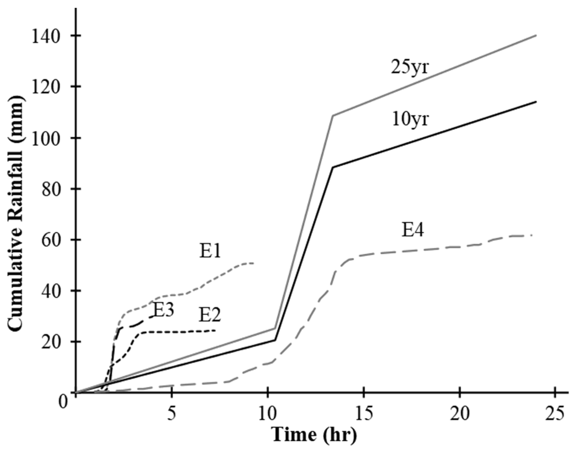
2.3.2. Single-Storm Simulations for Parameterization

Single-storm simulations with the WEPP were conducted using 15 min rainfall data to obtain runoff discharge values and sediment concentrations that could be delivered to the study ATIs. Six rainfall events (Figure 4) were simulated, with four of the events containing rainfall data measured during the growing season, i.e., June to September [22]. The two remaining events were Natural Resources Conservation Service (NRCS) TR-55 design events with 10- and 25-year return periods. These six events are within the representative distribution of the rainfall events for the region.

Each event was simulated using five different initial field conditions that were functions of time within the growing season. The initial conditions (

Table 1. Summary of initial condition parameters for the WEPP single-storm simulations.

Parameter	Range of Values
Days since last harvest (d)	280–347
Days since last tillage (d)	68–135
Cumulative rainfall since last tillage (mm)	561–1108
Bulk density after last tillage (g/cm3)	1.30–1.35
Initial canopy cover (0–100%)	8–98
Initial dead root mass (kg/m2)	0.025–0.131
Initial submerged residue (kg/m2)	0.096–0.307
Initial interrill cover (0–100%)	4.33–59.9
Initial rill cover (0–100%)	4.33–59.9

) included the cumulative rainfall since the last tillage, the bulk density after tillage, the degree of crop cover, and the rill/interrill cover. The multiple sets of rainfall and initial conditions provided a large representative range of possible runoff and sediment delivery rates to the ATIs.

Different combinations of rainfall events and initial field conditions were conducted to determine the depth of ponding at the ATI. The ponding depth was quantified using stage–discharge relationships, determined using the difference in flow volumes between the WEPP-simulated runoff and outflow through the drain tile. The WEPP’s impoundment module was used to mimic an ATI-WASCOB combination, which had a similar cross-sectional width and flow length as those at the Iowa County site.

Along with the ponding estimates, single-storm simulations were used to compute the sediment flux, calculated as the sediment yield mass divided by the duration of the rainfall event. The corresponding suspended sediment concentration value was then calculated using the sediment yield mass divided by the runoff volume of the event.

2.3.3. Continuous Modeling for Sediment and Longevity

Additionally, long-term model simulations were conducted using the WEPP at the three study sites in order to estimate the amount of time taken to drain different storm magnitudes. Continuous simulations were conducted for 100 years. Only the results from the last 50 years were used, as the first 50 years were for establishing steady-state conditions [21]. For these simulations, the hydraulic conductivity values measured during the permeameter studies were used for the segment of the hillslope that contained the ATI. Additionally, the surface impoundment module and the DRAINMOD extension were used in the continuous simulations.

2.3.4. Agricultural Conservation Planning Framework (ACPF)

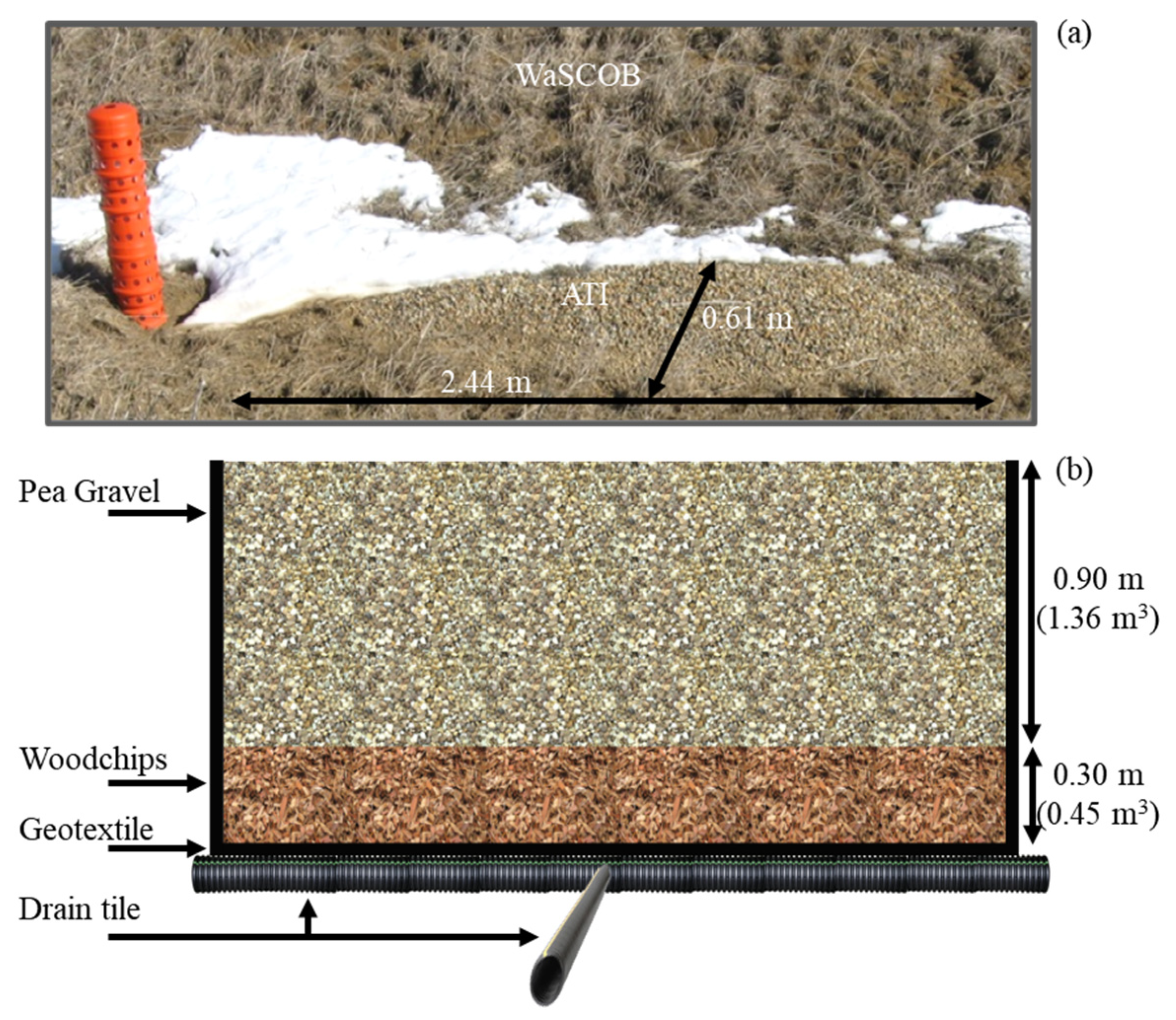
To assess potential implications that ATIs may have on overall watershed load reductions if implemented in certain locations, a watershed plan was developed using the Agricultural Conservation Planning Framework toolbox [28] for the Old Man’s Creek watershed, which is also within the Southern Iowa Drift Plain. This watershed was chosen due to the availability of more than 20 years of continuous stream nutrient and discharge data for quantifying the annual nutrient export loads at this watershed [29].

Following identification of all existing terraces and WASCOBs in this watershed using the Iowa BMP Mapping Project [30], the catchment tool developed by the Iowa Department of Natural Resources [26] was used to estimate the total watershed area that drains through these practices. Finally, the total loads and percent reductions were estimated considering the field monitoring results and in-stream data.

2.4. Lab

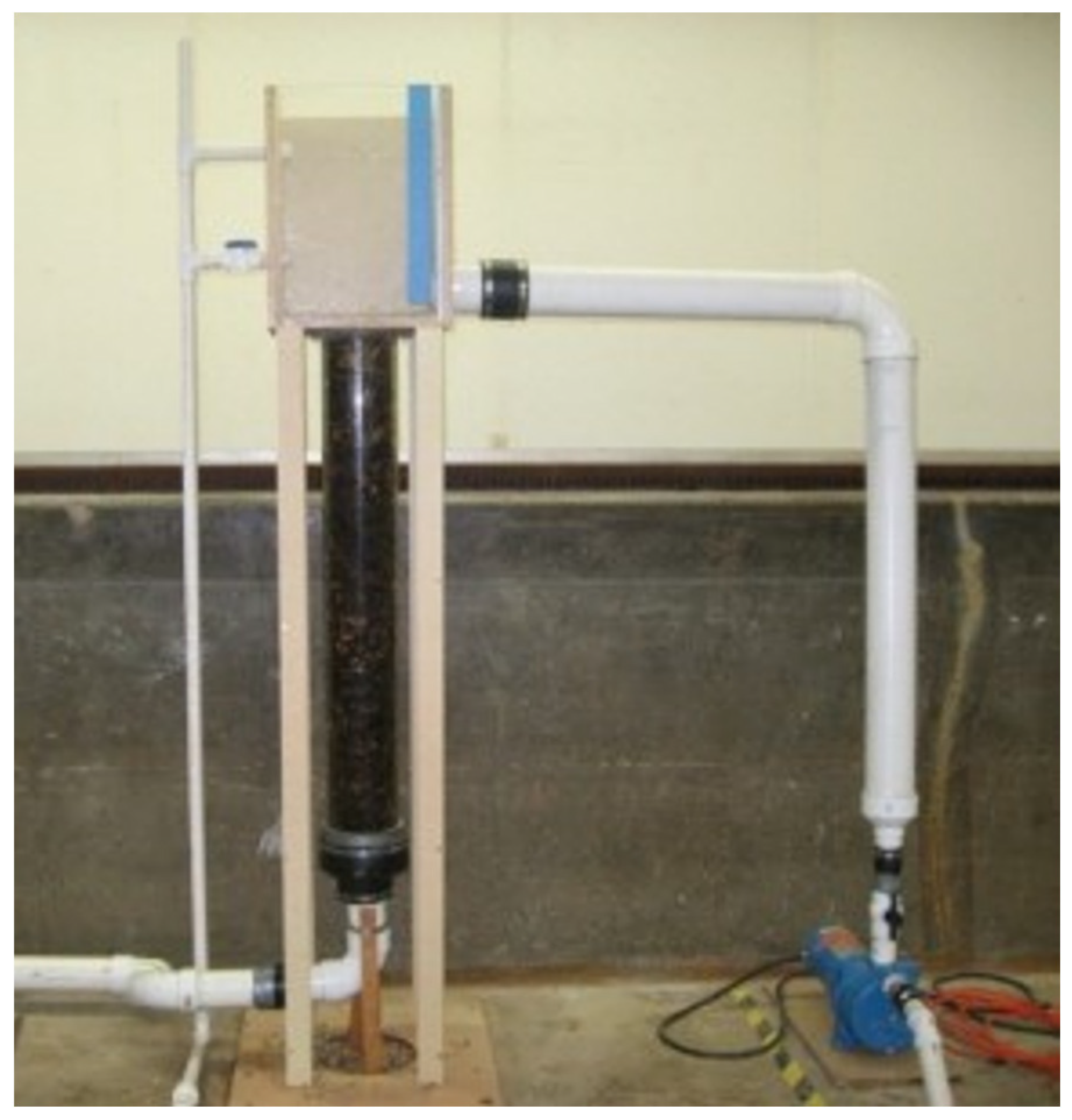
2.4.1. Permeameter Setup

A clear acrylic tube was used as a physical model of the ATI (Figure 5) in the laboratory. The physical model consisted of a head box, the permeameter (i.e., the acrylic column), a centrifugal pump, two inflow-regulating valves, PVC inflow/outflow pipes, an insertion flow meter with attached datalogger, a sediment auto-sampler, and an outlet valve. The permeameter had a length of 122 cm and a circular cross-sectional area of 198 cm².

A 1.5-horsepower, self-priming centrifugal pump delivered water from a 3.7 m³ sump to the head box. Two 5 cm Powell gate valves were used to regulate the flow from the centrifugal pump into the head box. Flow exiting the permeameter was diverted to another 1.78 m³ sump with an open drain at the bottom. A flow meter was connected to the outlet pipe for measuring the discharge through the permeameter.

2.4.2. Constant Head Tests for Hydraulic Conductivity

Constant head tests using the permeameter were devised to determine the time series of hydraulic conductivity for different combinations and arrangements (i.e., layered; mixed) of the woodchips and gravel. Before placement in the permeameter, the woodchips were allowed to saturate, and the pea gravel was washed to remove fine materials. The different media were poured into the permeameter at a steady rate and lightly packed. The masses of the fill media were recorded to determine the packing density.

Following packing, the permeameter was backfilled with water to prevent air bubbles from forming. Once the permeameter was purged of air, the centrifugal pump was started. The inflow and outflow valves were adjusted until a constant head of water, based on the single-storm simulations using the WEPP, was achieved. Cameras were focused on the head box to record changes in the head box during the experiment. Additionally, a flow meter on the outflow pipe was used to measure the instantaneous flow rate of the outflow. The discharge from the flow meter and the water level in the head box were used to determine the hydraulic conductivity with Darcy’s law.

2.4.3. Permeameter Experiments for Trapping Efficiency

For determining the trapping efficiency, the experimental procedure was identical to that of the constant head tests. Additionally, dry, pulverized sediment from the Iowa County hillslope was supplied to the permeameter through a feeder at a rate based on the WEPP single-storm simulations.

To measure the amount of sediment leaving the permeameter, an auto-sampler collected discrete samples of the total suspended solids from the pipe. Bucket samples were also collected from the outlet of the pipe.

The sediment delivery was paused to avoid overtopping when too much sediment caused the water to accumulate in the head box above 40 cm. Once the water level returned to its original level, the sediment delivery was resumed. Twenty-four hours after the conclusion of a series of sediment deliveries, the pea gravel and woodchips were removed from the permeameter, dried, and weighed.

2.5. Field Evaluation

2.5.1. Sampling Setup

Event monitoring of the installed ATIs was conducted during the growing seasons of 2013, 2019, and 2021. At the Iowa County site, the monitoring equipment included: a local weather station; a 7.62 m deep water table monitoring well; pressure transducers for measuring the ponding depth and flow through the drain tile; a still camera to capture the extent of ponding; water content reflectometers to measure the volumetric water content; a photo-electric erosion pin for determining the amount of deposited soil; and water–sediment autosamplers to collect runoff at the inlet and outlet of the ATI [16].

At the Keokuk and Wapello County sites (Figure 6), dual-tipping bucket rain gages equipped with a datalogger and cellular modem were installed to record precipitation and alert the research team when rainfall was occurring. Two sediment-and-water auto-samplers were installed at both sites to capture pre- and post-ATI runoff samples during a rain event. The water samplers were equipped with flow actuators to trigger sampling during runoff-producing rainfall events. Once triggered, each sampler collected 1 L samples at 10 min intervals for 4 h (24 samples in total). The actuators were installed within a 1 L surface sampling sump. The surface sump was intentionally sized the same as the sample collection volume to ensure that the sump was emptied, and new runoff water was being collected at each interval. For the pre-ATI runoff, the sumps were installed level with the land surface in locations where concentrated runoff and rill formation was present. The post-treatment sampler collected water from the base of the surface tile inlet, which was directly downstream of the ATI.

The flow rates through these ATIs were not measured, so the loads were not calculated. Using precipitation data collected on-site during each event and estimates of infiltration and surface runoff made using soil survey data [27], the flow through the ATIs was estimated; then, we estimated potential load reductions for each practice by incorporating our measured nutrient concentration reductions.

2.5.2. Gamma Spectroscopy

Finally, sediment cores collected at each site were sub-sectioned, dried, and lightly crushed. The sediment was then packed in Petri dishes and placed on a gamma spectroscopy system for ²¹⁰Pb age-dating analysis. The use of ²¹⁰Pb sediment profiles is a common geochronology technique used in deposition studies on floodplains and lakes, as seen in, e.g., [16]. This method is used to determine the age of the soil at a certain depth interval and involves comparing the established depth profile of the ²¹⁰Pb with patterns established using known/assumed deposition rates [31].

2.5.3. Lab Analyses for Sediment, Nitrogen, and Phosphorus

Immediately following an event during which the automatic samplers were triggered, samples were transported to a lab for analysis. All samples were analyzed for NO₃-N concentrations using a Nitratax, Hach, Loveland, CO, USA [32]. A subset of samples from each event was analyzed for ortho-phosphorous (OP) and total phosphorus (TP) content using the ascorbic acid method. All glassware used in the sampling and analysis of the dissolved reactive phosphorus was acid washed in 1 m hydrochloric acid. Instrument and reagent blanks were run daily and did not indicate significant levels of contamination. Lab instruments were calibrated with known concentration standard solutions according to the analytical protocols.

3. Results

3.1. Model Parameterization

The single-storm modeling simulations provided ponding depths and sediment concentrations delivered to the ATIs under different combinations of rainfall events and initial field conditions (

Table 2. Summary of single-storm numerical modeling simulations using the WEPP for runoff and sediment.

Data Source	No. of Simulated Events	Runoff Depth (cm)	Ponding Depth (cm)	Sediment Concentration (g/L)
Measured	140	1.9	0	11.5 (0.3–50.8)
Design storm	40	5.8	17.5 (14.4–20.7)	17.0 (4.1–50.5)

Notes: Adopted from [14]. Numbers in parentheses are the full range of values.

). Ponding was only observed during the two design storm simulations. For the 10-year design storm, the ponding depths ranged between 14.4 and 14.8 cm, while for the 25-year design storm event, the range was between 20.1 and 20.7 cm. The sediment concentration values for the events when ponding occurred ranged from 4.1 to 50.5 g/L, producing an average value of 17 g/L with a sediment flux of 18 g/s.

The simulated ponding depths and sediment concentrations were used to determine the level of water in the head box above the permeameter and the feed rate of sediment to the permeameter during the laboratory experiments. For the permeameter experiments, the “worst-case” conditions (i.e., the 25-year event) for the ponding depths and average sediment concentrations were used. The water level in the head box was set at 20 cm and the sediment delivery concentration was 17 g/L.

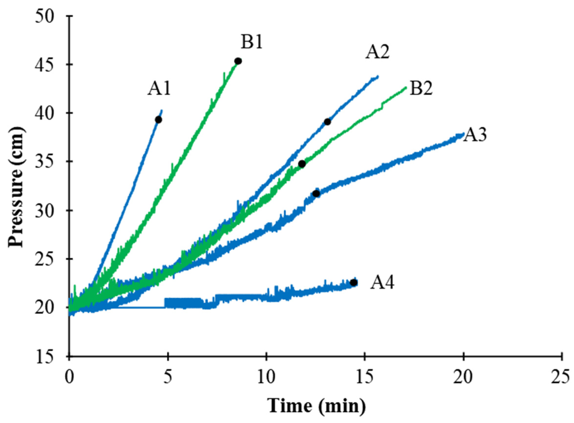
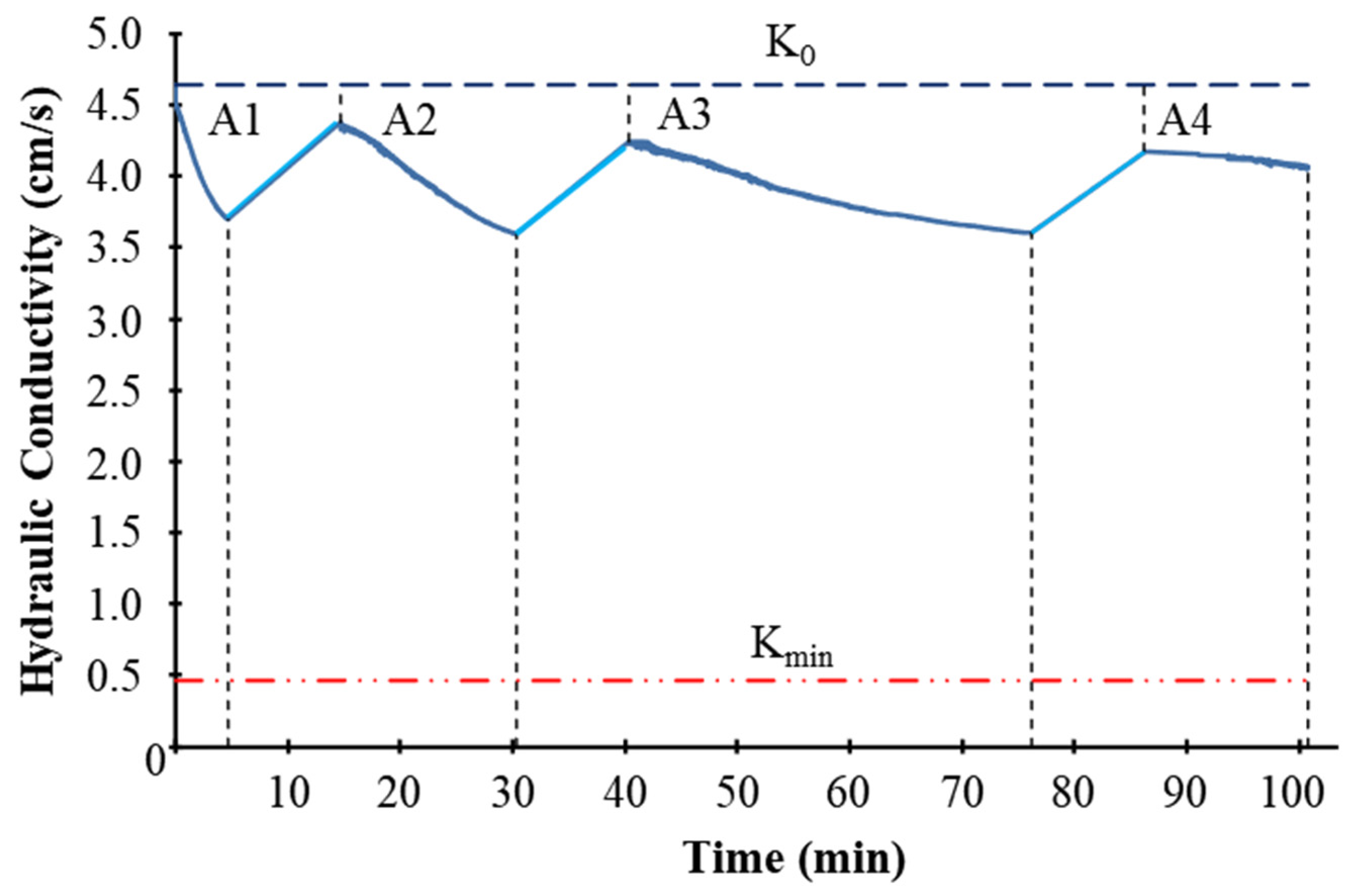
3.2. Permeameter Experiments

The constant-head permeameter experiments using a 100% gravel matrix had an average value of 5.34 cm/s ± 0.18 cm/s and the experiments using a 100% woodchip matrix had an average value of 4.76 cm/s ± 0.20 cm/s. These values correspond well with the ranges of values from other studies (e.g., gravel: 4.8–7.9 cm/s in [2,33]; woodchips: 2.7 to 11 cm/s in [34,35,36]). For the runs using the layered 0.90 m of pea gravel over 0.30 m of woodchips configuration, the average hydraulic conductivity value was 4.59 cm/s ± 0.36 cm/s, which was less than both of the 100% run averages.

When sediment was introduced to the permeameter, the largest accumulations of sediment (Figure 7) occurred in the transition areas of the permeameter, namely, the transition between the head box and the gravel, as well as the transition between the gravel and the woodchips. At the permeameter surface, 4290 g (58%) settled through ponding in the head box. This is similar to the 66% efficiency resulting from the ponding at slotted intakes [2]. Within the permeameter, an additional 2049 g (27%) of sediment was retained in the gravel and 1130 g (15%) in the woodchips. In this experiment, there was a proportional amount of sediment retained in the permeameter, highlighting the benefit of the ATI, where an additional 42% of the sediment was found.

Figure 8 shows the pressure head (or water level) time series for the head box during two sets of consecutive runs where sediment was fed to the permeameter. The blue lines (i.e., lines A1–A4 in Figure 8) represent the first series and the green lines (i.e., lines B1–B2 in Figure 8) represent the second series. Each line shows the pressure head increasing once the sediment is added at time = 0, as partial clogging of the gravel–woodchip matrix causes the water in the head box to pond. The sediment feed was discontinued after the depth in the head box rose above 40 cm in order to prevent overtopping. The black dots in Figure 8 mark the time when the sediment delivery ceased. The influx of clear water continued at half the original rate until the pressure head returned to 20 cm.

For each run, the lines in Figure 8 follow a concave-up shape while the sediment was delivered to the permeameter, as further clogging caused a faster increase in the ponding rate. Across the sets of curves, the time it took for the pressure head to reach a maximum level in the head box increased for each subsequent run. The slopes of the lines decrease as the runs progress from A1 to A4 and from B1 to B2.

Figure 9 shows how the hydraulic conductivity changes during the first set of experimental runs (A1–A4). The periods when K decreases correspond to the periods of sediment delivery to the head box. The periods when the hydraulic conductivity has a positive slope correspond to the periods when only clean water was added.

In addition, the maximum and the range of hydraulic conductivity values decreased across each consecutive run. Although the hydraulic conductivity values successively decreased as clogging enhanced, the values decreased less than 20%, which is far from the K_min threshold for functionality [2,33].

3.3. Field Monitoring

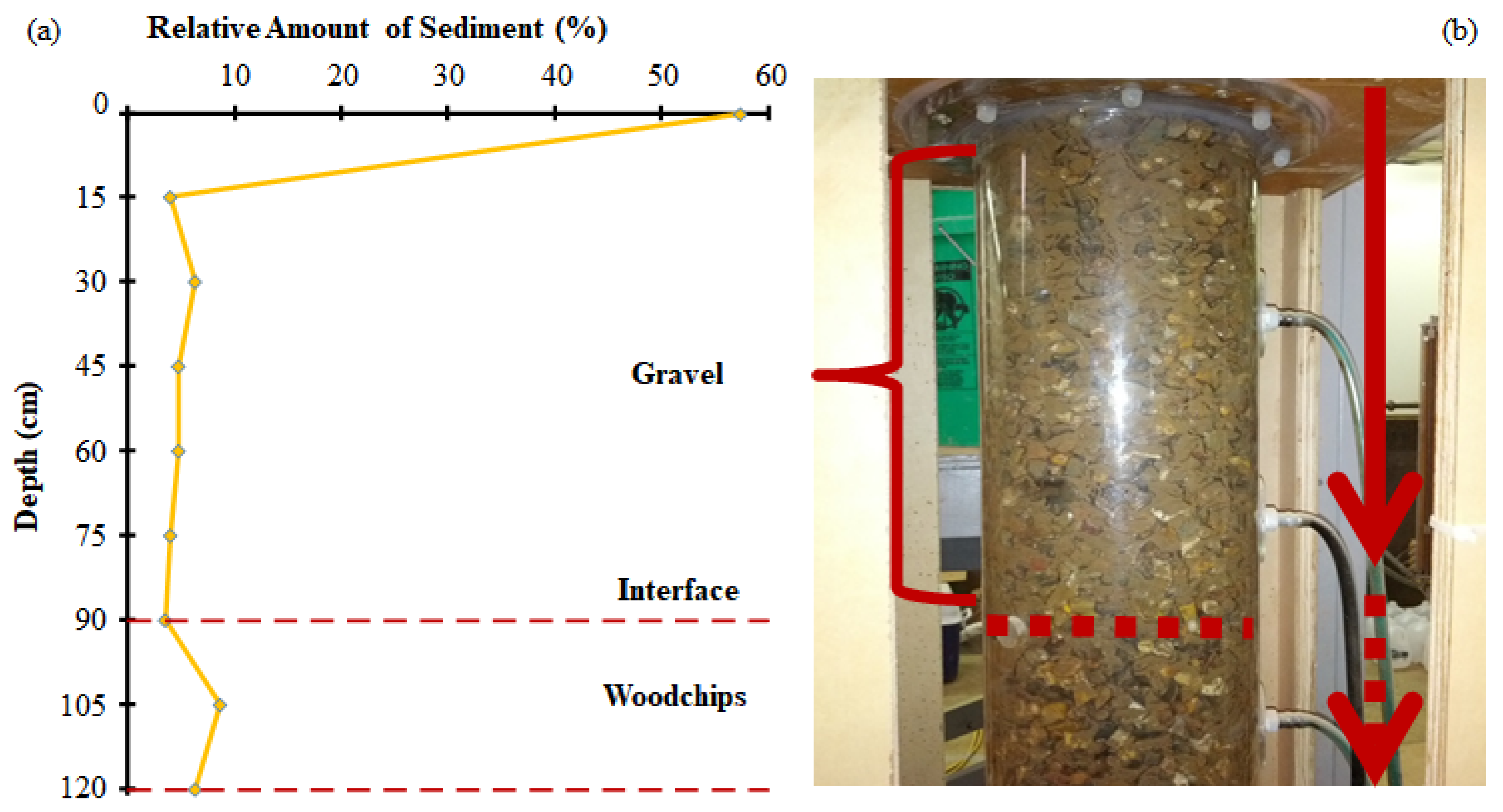
At the Iowa County site, one event was sampled on 24 June 2013, where nearly 2 inches of rain fell over a period of 15 h. Observations of ponding were made at this ATI site, as well as measurements of the depth of water (and thereby the discharge) in the outflow pipe (Figure 10). During this sampled event, the pressure transducer measured the flow-through of water in the drain tile and the autosampler collected the runoff.

To determine the drainage capacity, the discharge through the pipe was divided by the drainage area, and the value exceeded 1 in/d, the NRCS-recommended value. To determine the trapping efficiency of the sampled ATI, the total mass of sediment collected from the outlet pipe (Figure 10c), which was 105 kg, was compared against the WEPP-simulated influx of sediment to the ATI, which was 1054 kg. The ratio of the sediment efflux to the sediment influx was 1:10. As a result, the WASCoB-ATI was 90% effective at trapping the sediment delivered to it. A 90% trapping efficiency for the sediment would correspond to a proportional decrease in P loads. This efficiency is much greater than the efficiency for an orange slotted pipe of 66% [2].

The Keokuk and Wapello sites were monitored more extensively. More than 500 samples were collected at these sites over eight rain events in 2019 and 2021. On average, N concentrations were reduced from approximately 31 to 18 mg/L, or by 43%. Ortho-phosphorous (OP) concentrations were reduced by 9% on average, while total phosphorous (TP) was reduced by 14%. Although load reductions were not directly measured, coupling these concentration reductions with runoff modeling showed load reduction estimates of N, OP, and TP by 3.4, 0.02, and 0.47 kg/ha.

3.4. Cores

Due to the limited sampling at the Iowa County site, efforts were made to understand the long-term sedimentation rather than event monitoring. The amount of deposition over the ATI was measured by collecting cores from the soil surface to the surface of the gravel. Cores were taken along the 8-foot length of the ATI.

The amount of deposited sediment in front of the ATI ranged from 22 to 33 cm, which corresponds to deposition rates of 3.3 to 4.7 cm per year. This high deposition rate was confirmed when the cores were analyzed using gamma spectroscopy and fallout radionuclides to determine the geochronology of the erosion/deposition. The measured ²¹⁰Pb profiles (Figure 11) show that the average deposition rate was 5.44 ± 3.77 cm/yr. This value is not statistically different from the measured values when assessed using a standard t-test (p = 0.17).

3.5. Nutrient Monitoring Analysis

In 2019, four rain events were successfully monitored, while in 2021, an additional four events were monitored. NO₃-N concentrations were determined for all samples in both years. Ortho-phosphate and total phosphate contents were only analyzed in 2021. In 2019, the mean NO₃-N concentrations decreased from 16.4 ± 14.9 in the surface runoff to 8.8 ± 8.2 mg/L in the exit tile (

Table 3. Mean water quality results from 2019 and 2021 monitoring.

		n	NO3 (mg/L)	TP (mg/L)	OP (mg/L)
2019	Surface Runoff	132	16.4 ± 14.9	-	-
	Exit Tile	126	8.8 ± 8.2	-	-
2021	Surface Runoff	136	45.2 ± 12.7	2.4 ± 0.3	1.8 ± 0.2
	Exit Tile	135	25.8 ± 12.0	2.0 ± 0.2	1.6 ± 0.2

). In 2021, NO₃-N concentrations averaged 45.2 ± 12.7 in the surface runoff compared to 25.8 ± 12.0 mg/L in the exit tile (Table 3). Despite the different magnitudes between sampling years, the percent reductions were similar, being 46% in 2019 and 43% in 2021. In 2021, TP concentrations were reduced through the ATI by 17% from 2.4 ± 0.3 to 2.0 ± 0.2 mg/L, while OP concentrations were reduced by 13% from 1.8 ± 0.2 to 1.6 ± 0.2 mg/L.

3.6. Continuous Sediment Modeling

Table 4. Simulated drainage times of the ATIs.

Site	Drainage Area (ha)	Drain Time (d): 24 h 25 yr Event	Drain Time (d): 24 h 50 yr Event	Drain Time (d): 24 h 100 yr Event
Iowa	0.24	0.2	0.2	0.3
Keokuk	0.65	0.7	0.8	0.9
Wapello	1.4	0.9	1.0	1.1

lists the drainage times for the ATIs for the 24-h 25-year rainfall event (5.5 in); the 24-h 50-year rainfall event (6.0 in); and the 24-h 100-year rainfall event (6.5 in). A runoff coefficient of 0.5 was assumed. The drainage times for the ATIs ranged between 0.2 and 1.1 d. Only for the 24-h 100-year event at the Wapello site did it take more than 1 day to drain. The value of 1.1 day was still reasonable, so the ATIs seemed to be properly sized.

Table 5. Continuous WEPP modeling results.

Parameter	Iowa	Keokuk	Wapello
Runoff Volume (m3/ha/yr)	2515	1930	1995
Runoff Coefficient	0.27	0.21	0.22
Gross Erosion (T/ha/yr)	56.2	5.4	16.1
Net Erosion (T/ha/yr)	19.8	4.8	12.0
Exported Erosion (T/ha/yr)	0.3	0.6	3.2
Sediment Delivery Ratio	0.005	0.114	0.169
Sediment Trapping Efficiency	98%	87%	73%

details how much runoff and erosion was simulated along the hillslopes, as well as the trapping efficiencies of the combined ATI-WASCOB/terrace. The Iowa County site had relatively high runoff generation but low sediment generation along the hillslope. This translated to a high trapping efficiency. The modeled average trapping efficiency of 98% matched closely the measured trapping efficiency of 90% from the 2013 sampled event. The ATI-WASOB/terrace structures at the Keokuk County and Wapello County sites had lower efficiencies of 87% and 73%, respectively.

3.7. Nutrient Monitoring and ACPF Watershed Modeling Results

Combining the concentration reductions with the runoff modeling results, the estimated NO₃-N load reductions were 3.45 kg/ha, whereas the TP and OP reductions were 0.05 and 0.02 kg/ha, respectively (

Table 6. Load reduction estimates for each study site, the study site HUC-12 watersheds, and the Old Man’s Creek watershed.

		NO3-N	TP	OP
Load Reduction Rates	kg/ha	3.45	0.05	0.02
Total LR Keokuk ATI	kg	2.2	0.03	0.01
Total LR Wapello ATI	kg	4.8	0.07	0.03
Total LR Clear Creek, Keokuk	kg	4548	64	31
Total LR Soap Creek, Wapello	kg	2279	15	32
Total LR Old Man’s Creek	kg	14,856	2027	-
Old Man’s Creek Reduction	%	1.6	1.4	-

). Based on the catchment areas monitored at the Keokuk and Wapello sites, this load reduction equates to mass reductions of 2.2, 0.03, and 0.01 kg for the NO₃-N, TP, and OP removed at the Keokuk site, respectively, and 4.8, 0.07, and 0.03 kg for the NO₃-N, TP, and OP removed at the Wapello site, respectively.

Watershed scale nutrient reductions were estimated by assuming that the mass reductions measured within a single field are the same for all potential ATI locations in the watershed. Hence, if ATIs were to be implemented at all terrace locations within the Indian Creek watershed in Keokuk County, approximately 4548, 64, and 31 kg of NO₃-N, TP, and OP would have been captured through this practice. In the Soap Creek watershed of Wapello County, the same assumptions would equate to reductions of 279, 15, and 32 kg for NO₃-N, TP, and OP, respectively. Estimating a percent load reduction for this mass removal in these two watersheds is not possible since stream discharge and nutrient data were not available in these watersheds. If the load reduction from this ATI was applied to the nearby 63,847 ha watershed at Old Mans Creek, where loading data are available, we estimate that approximately 14,856 kg (1.6%) of total stream NO₃-N and 2027 kg (1.4%) of total stream TP could be captured if ATIs were installed.

The estimated NO₃-N reductions achieved through the ATI practice were lower than for other tile drainage BMPs reported in the Iowa Nutrient Reduction Strategy (INRS), such as in, e.g., [37]: bioreactors, 43 ± 21%; drainage water management, 33 ± 32%; wetlands, 52%; saturated buffers, 50 ± 13%; and multipurpose oxbows, 45%. The TP load reductions were also much lower than those reported in the INRS, but it is important to note that these TP practices were mainly associated with suspended sediment reductions. Specific OP reductions have not been reported previously.

4. Discussion

ATIs were designed to increase the effective hydraulic retention time of sediment-and-nutrient-laden runoff, thereby optimizing the potential for ponding, sedimentation, filtration, and denitrification. The permeameter experiments conducted here allowed for observing the flow through different ATI matrices to see which configuration produced the greatest reductions.

Despite the different sizes and compositions, the two media had similar hydraulic conductivities, at 5.34 cm/s ± 0.18 cm/s for the 100% gravel matrix and 4.76 cm/s ± 0.20 cm/s for the 100% woodchip matrix. However, for the runs using the layered configuration with 0.90 m of pea gravel over 0.30 m of woodchips, the average hydraulic conductivity (4.59 cm/s ± 0.36 cm/s) was less than both the 100% run averages because of the developed complex flow pathways, especially at different interfaces. Hydraulic conductivity is not just a function of the media’s grain size distribution, but also their average width, shape, and tortuosity [38]. The additional slowing of the runoff flux achieved by adding different interfaces helped to increase the effective hydraulic retention time.

The effect of the interfaces was also apparent in the sediment experiments with the permeameter. When sediment was introduced to the permeameter, the largest accumulations of sediment occurred at the transition between the head box and the gravel and the transition between the gravel and the woodchips (Figure 7). Although, the characteristics of the woodchips resulted in only a 10% decrease in the hydraulic conductivity, as more sediment per unit length of the permeameter was trapped within the woodchip layer due to more-complex flowpaths. The flow velocity is related to the square of the friction, i.e., the Darcy–Weisbach equation.

As the permeameter pore spaces filled with sediment, the porosity in the gravel–woodchip matrix further decreased the hydraulic conductivity [39]. This was seen with the decreasing slopes of the lines A1–A4 and B1–B2 in Figure 8. Each successive run took longer to reach its cutoff point than the preceding run. In addition, the maximum and the range of hydraulic conductivity values decreased across consecutive runs. The lower maximum values signified the gradual clogging of the permeameter. The smaller ranges showed the movement towards a steady state as the sediment plug moved further through the permeameter and dispersed more evenly.

The results from the field monitoring and long-term continuous modeling simulations supported the permeameter experiments. Both approaches confirmed that the drainage capacity of the ATIs exceeded 1 in/d, which is the NRCS recommended value. The measured sediment trapping efficiency was at 90%, while the modeled average trapping efficiencies were between 73% and 98%. The high trapping efficiency corresponded to measured deposition rates of 5.44 ± 3.77 cm/yr. The sampling at the Keokuk County and Wapello County ATI sites also showed a reduction in nutrient concentrations in the runoff moving through the ATIs. On average, N concentrations were reduced by approximately 43%.

Research has shown that bioreactors with woodchip carbon sources provide substantial NO₃-N removal from tile drainage water [40]. Nitrate removal rates can vary considerably, as field-based studies indicate bioreactors can reduce annual NO₃-N loads by 23–98% [41]. The Iowa Nutrient Reduction Strategy reported the average NO₃-N reduction from bioreactors to be 43%.

Longer retention times correlate with higher nitrate removal rates, with retention times of 2–10 days resulting in removal efficiencies of up to 30–100% [40]. The retention times associated with ATIs would be considerably shorter (minutes to hours, as seen through the lab experiments and limited field studies), so less nitrate removal would be expected with these systems. Testing a wider range of flow and sediment conditions, both in the lab and the field, is needed to confirm these times. For example, [34] reported nitrate reductions of 10–40% with retention times less than five hours.

As the sediment slugs progress through the ATI with each successive event, the retention times of the flow and sediment increase. This delay allows for further denitrification. If needed, flushing the gravel with clear water may decrease the retention time temporarily, which would prolong the ATI’s lifetime.

The layered medium of pea gravel and woodchips in the permeameter was difficult to completely clog with sediment. For just gravel inlets, the expected lifespans have been determined to be at least 10 years [42]. The preliminary modeling efforts in this study suggest that it would take 75 25-year events to clog the permeameter [14]. At our field sites, the ATIs have continued to function from June 2011 to the present time without any noticeable problems.

5. Conclusions

Through different approaches, i.e., computational, experimental, and field methods, this study disclosed a potential benefit of replacing existing slotted-pipe inlets with an ATI consisting of a layered gravel–woodchip filter. The ATI primarily traps sediment and attached phosphorus through runoff ponding and enhanced sediment settling around the intake. The gravel further filters the sediment and its contained nutrients as the runoff passes through the ATI. The woodchips are an innovative addition that facilitates nitrate breakdown, like a denitrifying wall or a bioreactor.

Herein, the ATIs were used as a support practice for terraces and WASCoBs. This coupling increases their overall efficiency at retaining soil that would otherwise pass freely through conventional open or slotted intakes. In addition, an ATI can be a standalone practice in low-relief areas with poorly drained soils. Due to their low profile, farmers can pass freely over ATIs, unlike with the slotted-pipe intakes.

Our constant-head permeameter experiments showed that the average hydraulic conductivity of the layered gravel–woodchip was less than both of the 100% run averages because of the developed complex flow pathways, especially at different interfaces. The additional slowing of the runoff flux helped to increase the effective hydraulic retention time, thus optimizing the potential for denitrification.

The effect of the interfaces was also apparent in the sediment experiments with the permeameter. Within the permeameter, an additional 2049 g (27%) of sediment was retained in the gravel and 1130 g (15%) in the woodchips.

In addition, the maximum and the range of hydraulic conductivity values decreased across consecutive runs. The decreasing maximum values signify the gradual clogging of the permeameter, while the decreasing range suggests that less sediment is being flushed and that the sediment is sitting in the permeameter longer.

Our field monitoring also showed that the drainage capacity of the ATIs exceeded 1 in/d, the NRCS recommended value. The trapping efficiency of the WASCoB-ATI was at 90%, which is much greater than the efficiency for an orange slotted pipe of 66% [2]. This high trapping efficiency corresponds to deposition rates of 5.44 ± 3.77 cm/yr.

At the Keokuk County and Wapello County ATI sites, more than 500 runoff samples were collected over eight rain events, which were then analyzed for their nitrogen and phosphorus content. On average, N concentrations were reduced from approximately 31 to 18 mg/L, or 43%. The OP concentrations were reduced by 9% on average, and the TP was reduced by 14%. These concentration reductions were estimated to reduce loads of N, OP, and TP by 3.4, 0.02, and 0.47 kg/ha, respectively.

Finally, our long-term continuous modeling simulations estimated that the amount of time taken to drain even a 100-year design storm was less than 1.1 d with the ATIs. The modeled average trapping efficiency was 98% at the Iowa County site. The structures at the Keokuk and Wapello sites had lower efficiencies of 87% and 73%, respectively.

Coupling WASCOBs and terraces with ATIs will make them more efficient at preventing soil from passing freely through conventional open or slotted-pipe intakes. ATIs will also reduce the dissolved nutrient loading to local streams and improve downstream water quality.

References

1. Karlen, D.L.; Tomer, M.D.; Neppel, J.; Cambardella, C.A. A preliminary watershed scale soil quality assessment in north central Iowa, USA. Soil Tillage Res. 2008, 99, 291–299. [Google Scholar] [CrossRef]
2. Wilson, B.N.; Nguyen, H.V.; Singh, U.B.; Morgan, S.; Van Buren, P.; Mickelson, D.; Jahnke, E.; Hansen, B. Evaluations of Alternative Designs for Surface Tile Inlets Using Prototype Studies: A Final Report to the Minnesota Department of Agriculture; Biosystems and Agricultural Engineering Department and St. Anthony Falls Laboratory, University of Minnesota: Minneapolis, MN, USA, 1999. [Google Scholar]
3. Blann, K.L.; Anderson, J.L.; Sands, G.R.; Vondracek, B. Effects of agricultural drainage on aquatic ecosystems: A review. Crit. Rev. Environ. Sci. Technol. 2009, 39, 909–1001. [Google Scholar] [CrossRef]
4. Boland-Brien, S.J.; Basu, N.B.; Schilling, K.E. Homogenization of spatial patterns of hydrologic response in artificially drained agricultural catchments. Hydrol. Process. 2014, 28, 5010–5020. [Google Scholar] [CrossRef]
5. Jaynes, D.B.; Hatfield, J.L.; Meek, D.W. Water quality in Walnut Creek watershed: Herbicides and nitrate in surface waters. J. Environ. Qual. 1999, 28, 45–59. [Google Scholar] [CrossRef]
6. Jones, C.S.; Davis, C.A.; Drake, C.W.; Schilling, K.E.; Debionne, S.H.; Gilles, D.W.; Demir, I.; Weber, L.J. Iowa statewide stream nitrate load calculated using in situ sensor network. J. Am. Water Resour. Assoc. 2018, 54, 471–486. [Google Scholar] [CrossRef]
7. King, K.W.; Williams, M.R.; Fausey, N.R. Contributions of systematic tile drainage to watershed-scale phosphorus transport. J. Environ. Qual. 2015, 44, 486–494. [Google Scholar] [CrossRef] [PubMed]
8. Smith, D.R.; King, K.W.; Johnson, L.; Francesconi, W.; Richards, P.; Baker, D.; Sharpley, A.N. Surface runoff and tile drainage transport of phosphorus in the midwestern United States. J. Environ. Qual. 2015, 44, 495–502. [Google Scholar] [CrossRef]
9. Schilling, K.E.; Streeter, M.T.; Isenhart, T.M.; Beck, W.J.; Tomer, M.D.; Cole, K.J.; Kovar, J.L. Distribution and mass of groundwater orthophosphorus in an agricultural watershed. Sci. Total Environ. 2018, 625, 1330–1340. [Google Scholar] [CrossRef]
10. Iowa Department of Agriculture and Land Stewardship. Iowa Nutrient Reduction Strategy: A Science and Technology-Based Framework to Assess and Reduce Nutrients to Iowa Waters and the Gulf of Mexico; Iowa Department of Agriculture and Land Stewardship: Ames, IA, USA, 2017.
11. Miller, T.P.; Peterson, J.R.; Lenhart, C.F.; Nomura, Y. The Agricultural BMP Handbook for Minnesota; Minnesota Department of Agriculture: St. Paul, MN, USA, 2012. [Google Scholar]
12. Shipitalo, M.J.; Tomer, M.D. Quantifying the Effects of Alternative Surface Inlet Protection Strategies on Water Quality: Leopold Center Completed Grant Report #478; Leopold Center for Sustainable Agriculture: Ames, IA, USA, 2015. [Google Scholar]
13. Williams, M.; Livingston, S.J.; Penn, C.J.; Gonzalez, J.M. Hydrologic assessment of blind inlet performance in a drained closed depression. J. Soil Water Conserv. 2020, 75, 352–361. [Google Scholar] [CrossRef]
14. Ettema, W.D. Alternative Tile Intake Design for Intensively Managed Agro-Ecosystems. Master’s Thesis, University of Iowa, Iowa City, IA, USA, 2014. [Google Scholar]
15. Anders, A.M.; Bettis, E.A.; Grimley, D.A.; Stumpf, A.J.; Kumar, P. Impacts of quaternary history on critical zone structure and processes: Examples and a conceptual model from the Intensively Managed Landscapes Critical Zone Observatory. Front. Earth Sci. 2018, 6, 24. [Google Scholar] [CrossRef]
16. Wilson, C.G.; Abban, B.K.B.; Keefer, L.L.; Wacha, K.M.; Dermisis, D.C.; Giannopoulos, C.P.; Zhou, S.; Goodwell, A.E.; Woo, D.K.; Yan, Q.; et al. The Intensively Managed Landscape Critical Zone Observatory: A scientific testbed for agroecosystem functions and services. Vadose Zone J. 2018, 17, 1–21. [Google Scholar] [CrossRef]
17. Iowa State University. Iowa Environmental Mesonet. Available online: http://mesonet.agron.iastate.edu/ (accessed on 15 January 2023).
18. Cruse, R.; Flanagan, D.; Frankenberger, J.; Gelder, B.; Herzmann, D.; James, D.; Krajewski, W.; Kraszewski, M.; Laflen, J.; Opsomer, J. Daily estimates of rainfall, water runoff, and soil erosion in Iowa. J. Soil Water Conserv. 2006, 61, 191–199. [Google Scholar]
19. Gelder, B.; Sklenar, T.; James, D.; Herzmann, D.; Cruse, R.; Gesch, K.; Laflen, J. The Daily Erosion Project-daily estimates of water runoff, soil detachment, and erosion. Earth Surf. Process. Landf. 2017, 43, 1105–1117. [Google Scholar] [CrossRef]
20. Iowa State University. Daily Erosion Project. Available online: https://www.dailyerosion.org/map/#20190328/qc_precip/-94.50/42.10/6//0/ (accessed on 31 December 2020).
21. Papanicolaou, A.N.; Abaci, O. Upland erosion modeling in a semihumid environment via the water erosion prediction project model. J. Irrig. Drain. Eng. 2008, 134, 796–806. [Google Scholar] [CrossRef]
22. Dermisis, D.; Abaci, O.; Papanicolaou, A.N.; Wilson, C.G. Evaluating grassed waterway efficiency in southeastern Iowa using WEPP. Soil Use Manag. 2010, 25, 183–192. [Google Scholar] [CrossRef]
23. Flanagan, D.C.; Nearing, M.A. Water Erosion Prediction Project: Hillslope Profile and Watershed Model Documentation: NSERL Report No. 10; USDA-ARS National Soil Erosion Research Lab: West Lafayette, IN, USA, 1995.
24. Oztekin, T.; Brown, L.C.; Fausey, N.R. Modification and evaluation of the WEPP hillslope model for subsurface drained cropland: Paper No: 042274. In Proceedings of the 2004 ASAE/CSAE Annual International Meeting, Ottawa, ON, Canada, 1–4 August 2004. [Google Scholar]
25. Foster, G.R.; Flanagan, D.C.; Nearing, M.A.; Lane, L.J.; Risse, L.M.; Finkner, S.C. Hillslope Erosion Component (Chapter 11). In Water Erosion Prediction Project: Hillslope Profile and Watershed Model Documentation, NSERL Report No. 10; Flanagan, D.C., Nearing, M.A., Eds.; USDA-ARS National Soil Erosion Research Laboratory: West Lafayette, IN, USA, 1995; pp. 1–12. [Google Scholar]
26. Asell, A. Catchment Tools; Iowa Department of Natural Resources: Ames, IA, USA, 2019.
27. Soil Survey Staff (U.S. Department of Agriculture, Natural Resources Conservation Service). Web Soil Survey. Available online: http://websoilsurvey.nrcs.usda.gov (accessed on 15 January 2023).
28. U.S. Department of Agriculture. Agricultural Conservation Planning Framework. Available online: https://acpf4watersheds.org/toolbox/#soils (accessed on 15 April 2019).
29. Iowa Department of Natural Resources. AQuIA. Available online: https://programs.iowadnr.gov/aquia/ (accessed on 15 March 2019).
30. Iowa State University. Iowa BMP Mapping Project. Available online: https://www.iowaview.org/iowa-conservation-mapping-project/ (accessed on 15 April 2019).
31. Appleby, P.G.; Oldfield, F. The calculation of lead-210 dates assuming a constant rate of supply of unsupported 210Pb to the sediment. Catena 1978, 5, 1–8. [Google Scholar] [CrossRef]
32. Hach. Nitratax. Available online: https://www.hach.com/nitrate-sensors/nitratax-sc-nitrate-sensors/family?productCategoryId=35546907021&_bt=356464702016&_bk=&_bm=b&_bn=g&utm_id=go_cmp-370746550_adg-24428698030_ad-356464702016_dsa-874297212215_dev-c_ext-_prd-&utm_source=google&gclid=CjwKCAiAwrf-BRA9EiwAUWwKXpooBrmN898_mYCN4IPdXHgcnz0WcKU29MFfmtOStcECndjk2LeCrhoCkqUQAvD_BwE (accessed on 31 December 2020).
33. Oveson, K.L. Evaluation and Design of Rock Inlets as an Alternative form of Surface Drainage. Master’s Thesis, University of Minnesota, Minneapolis, MN, USA, 2001. [Google Scholar]
34. Christianson, L.E.; Bhandari, A.; Helmers, M.J. A practice-oriented review of woodchip bioreactors for subsurface agricultural drainage. Appl. Eng. Agric. 2012, 28, 861–874. [Google Scholar] [CrossRef]
35. Chun, J.A.; Cooke, R.A.; Eheart, J.W.; Kang, M.S. Estimation of flow and transport parameters for woodchip based bioreactors: I. Laboratory-scale bioreactor. Biosyst. Eng. 2009, 104, 384–395. [Google Scholar] [CrossRef]
36. Verma, S.; Bhattarai, R.; Goodwin, G.; Cooke, R.; Chun, J.A. Evaluation of Conservation Drainage Systems in Illinois: Bioreactors. ASABE Paper No. 10098942010; American Society of Agricultural and Biosystems Engineering: St. Joseph, MI, USA, 2010. [Google Scholar]
37. Iowa State University. Tracking the Iowa Nutrient Reduction Strategy: Interactive Data Dashboards. Available online: https://nrstracking.cals.iastate.edu/tracking-iowa-nutrient-reduction-strategy (accessed on 3 January 2024).
38. Hillel, D. Environmental Soil Physics; Academic Press: San Diego, CA, USA, 1998. [Google Scholar]
39. Sakthivadivel, R.; Einstein, H.A. Clogging of porous column of spheres by sediment. J. Hydraul. Div. ASCE 1970, 96, 461–472. [Google Scholar] [CrossRef]
40. Greenan, C.M.; Moorman, T.B.; Parkin, T.B.; Kaspar, T.C.; Jaynes, D.B. Denitrification in wood chip bioreactors at different water flows. J. Environ. Qual. 2009, 38, 1664–1671. [Google Scholar] [CrossRef]
41. Ranaivoson, A.Z.H. Effect of Fall Tillage Following Soybeans and the Presence of Gravel Filters on Runoff Losses of Solids, Organic Matter, and Phosphorus on a Field Scale. Ph.D. Thesis, University of Minnesota, St. Paul, MN, USA, 2004. [Google Scholar]
42. Feyereisen, G.W.; Francesconi, W.; Smith, D.R.; Papiernik, S.K.; Krueger, E.S.; Wente, C.D. Effect of replacing surface inlets with blind or gravel inlets on sediment and phosphorus subsurface drainage losses. J. Environ. Qual. 2015, 44, 594–604. [Google Scholar] [CrossRef] [PubMed]
43. Wilson, C.G.; Wacha, K.M.; Papanicolaou, A.N.; Sander, H.A.; Freudenberg, V.B.; Abban, B.K.B.; Zhao, C. Dynamic Assessment of Current Management in an Intensively Managed Agroecosystem. J. Contemp. Water Res. Educ. 2016, 158, 148–171. [Google Scholar] [CrossRef]
44. Duffy, M.D. Value of Soil Erosion to the Landowner. Ag Decision Maker. A1-75. 2012. Available online: https://www.extension.iastate.edu/agdm/crops/html/a1-75.html (accessed on 6 January 2022).
Figure 1. An alternative tile intake consisting of a buried column of gravel over a layer of woodchips. Blue arrows represent flowpaths of water. The blue, irregular shapes represent ponding of water.
Water 16 00309 g001
Figure 2. The study sites are in the state of Iowa, USA. The gray area is the Southern Iowa Drift Plain region. The colored shapes are the sub-watersheds where the ATIs were installed.
Water 16 00309 g002
Figure 3. (a) An installed ATI at the Iowa County site. At the surface, only the pea gravel is visible. The orange pipe was left as a safety precaution. The holes on the lower half were blocked. (b) A vertical cross section of the ATI with 0.90 m of gravel over 0.30 m of woodchips.
Water 16 00309 g003
Figure 4. Characterization of the six rainfall events used in the WEPP single-storm simulations: e.g., total rainfall, event duration, and changes in intensity. Events E1–E4 are measured events from monitoring sites near the ATIs. The “10 yr” and “25 yr” labels represent the 10-year 24 h and 25-year 24 h events of the NRCS TR-55 method, respectively.
Water 16 00309 g004
Figure 5. Physical model of an ATI. This permeameter was developed to determine the effective hydraulic conductivity of the ATI and quantify its filtering efficiency through the pea gravel and woodchips.
Water 16 00309 g005
Figure 6. The monitoring equipment placed at the Keokuk County site.
Water 16 00309 g006
Figure 7. (a) Mass of deposited sediment in the permeameter after all runs. (b) Visible intrusion of sediment following a sediment test. Arrows indicate direction of flow.
Water 16 00309 g007
Figure 8. Head box pressure (or, equivalently, the depth of water) during the sediment flux experiments.
Water 16 00309 g008
Figure 9. Time series of hydraulic conductivity, K, over consecutive runs. The initial hydraulic conductivity of the gravel–woodchip matrix, K0, averaged 4.59 cm/s ± 0.36 cm/s. The minimum hydraulic conductivity value (Kmin) is considered the minimum value at which water passes through the matrix. The value for Kmin of 0.10 × K0 was adopted from [2,33].
Water 16 00309 g009
Figure 10. Sampled runoff event. (a) A rill that formed delivered water to the ATI. (b) Ponding near the control intake. (c) Water depth measured with the pressure transducer in the drain tile below the ATI. The maximum depth of 4.5 cm corresponds to 35.4% of the pipe cross-sectional area.
Water 16 00309 g010
Figure 11. Sediment deposition rates. (a) Deposition rates over the Iowa County ATI, determined using the 210Pb profile. The x-axis depicts the activity of the 210Pb in Becquerels per gram (Bq/g). (b) The Iowa County ATI in 2021, which was 10 years after its installation. The “×” symbols show where cores were collected. The arrow shows the main flow path over the ATI. The values in white are the depth measurements at the nearest “×”.
Water 16 00309 g011