Article

Performance of Reynolds Averaged Navier–Stokes and Large Eddy Simulation Models in Simulating Flows in a Crossflow Ultraviolet Reactor: An Experimental Evaluation

School of Civil and Environmental Engineering, Nanyang Technological University, 50 Nanyang Avenue, Singapore 639798, Singapore
*
Author to whom correspondence should be addressed.
Water 2024, 16(2), 271; https://doi.org/10.3390/w16020271
Submission received: 16 December 2023 / Revised: 9 January 2024 / Accepted: 10 January 2024 / Published: 12 January 2024
(This article belongs to the Special Issue CFD in Fluid Machinery Design and Optimization)

Abstract

:
Computational Fluid Dynamics (CFD) has been increasingly adopted as a design tool for the simulation of UV disinfection efficiency and the optimization of the configuration of a UV reactor. However, the performance of CFD with different turbulence closures may vary significantly. In the present study, an experimental evaluation was performed to assess the performance of CFD with five Reynolds Averaged Navier–Stokes (RANS) turbulence closures and three Large Eddy Simulation (LES) sub-grid scale (SGS) models. A simplified crossflow reactor with a single lamp sleeve was fabricated for the experimental measurements and numerical simulations. Overall, the superior performance of LES compared to RANS models in flow predictions within a complex configuration is demonstrated.

1. Introduction

Ultraviolet (UV) disinfection, as an alternative among the assortment of treatment methods, has shown high efficiency in water, wastewater, and ballast water treatments [1]. The microbial inactivation inside a UV reactor is governed by the total amount of UV light that the microorganism receives, namely the UV exposure dose. Thus, both the UV light intensity distribution and water flow prediction are needed for the calculation of the UV dose. In the past few decades, integral approaches to UV disinfection simulation have been commonly employed, which consist of a fluence rate model for UV light intensity distribution, a numerical model for flow prediction, and a microbial inactivation kinetic model for the fluence response of target microorganisms. These models have been extensively studied individually [2,3,4,5] and systematically [6,7,8,9]. Among these studies, Computational Fluid Dynamics (CFD) has been commonly adopted as a powerful numerical model for flow prediction to predict the performance of a UV reactor and to conduct the configurational optimization [6,7,8,9,10,11,12,13,14].
Despite the increasing adoption of CFD, it is worth noting that flow prediction is challenging due to the complex flow pattern inside compact UV reactors with many UV cylindrical lamps [7,15,16]. As far as we are aware, Liu et al. [7] first showed that the efficiency of a disinfection reactor is sensitive to the RANS turbulence model selection. Wols et al. [15] further investigated the performance of CFD simulations by comparing the standard k-epsilon turbulence model and Large Eddy Simulation (LES) with experimental measurements. LES was found in their study to predict disinfections better than RANS models. Zhang et al. [16] pointed out in their review work that unsteady flow structure effects and the complexity of reaction systems are key challenges for disinfection process simulations. Shah et al. [17] summarized the CFD performances in previous studies and again pointed out the reduced accuracy of RANS in flow predictions within UV reactors. Despite the reduced accuracy of RANS with certain turbulence models, studies using RANS models [11,12,18,19,20,21,22,23], however, remained the dominant approach for UV reactor simulations in recent decades due to their efficiency. We note particularly that correct simulations of flow separation around cylindrical UV lamps are key to the improvement of numerical accuracy. Recently, an inspiring study by Bose and Yeo [24] on atmospheric boundary layer flow problems again demonstrated the weakness of RANS models in predicting the flow separation behind a smooth hill, which is comparable to the flow behind a UV lamp. All in all, the usage of RANS models for UV disinfection simulations could result in the reduced accuracy of flow predictions as well as consequent inactivation efficiency. Therefore, it is necessary to evaluate the performance of the RANS and LES models for a satisfactory prediction inside complex UV reactors in order to develop an improved understanding of the tradeoff.
In the present study, we performed an experimental validation for five RANS turbulence closures (models) and three LES sub-grid scale (SGS) models, all of which are well-developed and commonly used models. A typical configuration of the UV disinfection for ballast water treatments is a closed crossflow reactor with UV lamp sleeves usually placed perpendicular to the flow with a staggered pattern, which involves the wall interaction. Therefore, a customized closed conduit in which the flow passed a horizontally orientated cylindrical sleeve was adopted for measurements of the velocity field with the approach of Particle Image Velocimetry (PIV). The experimental and numerical methodologies are described in Section 2 and Section 3, respectively. The results and discussion are presented in Section 4. Finally, conclusions are drawn in Section 5.

2. Experimental Methodology

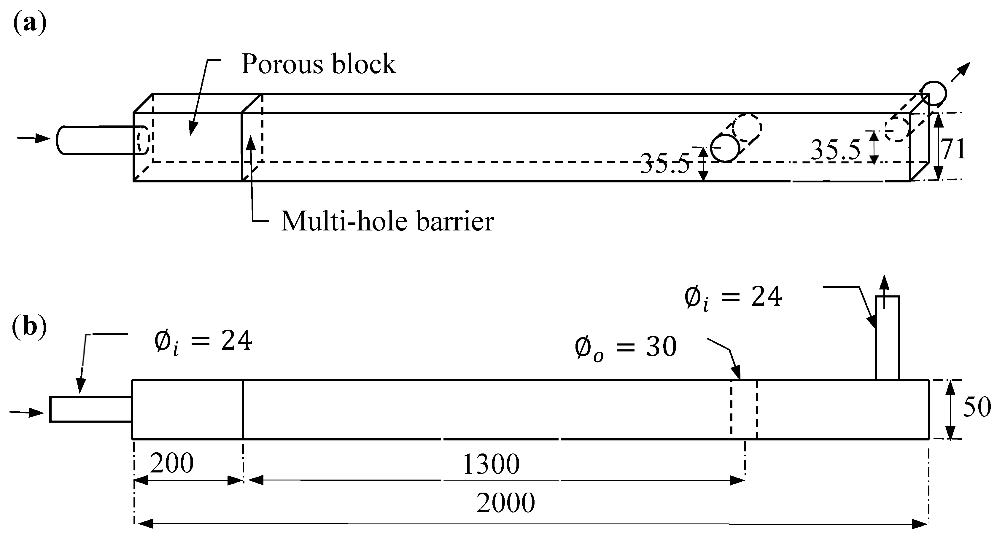
2.1. Experimental Setup

A lab-scale model was fabricated (Zoncepz Solutions, Singapore, Singapore) using transparent acrylic sheets with a thickness of 10 mm to quantify the hydrodynamics behind the single lamp sleeve of crossflow UV reactors. As illustrated in Figure 1, the cylinder (sleeve) had an outer diameter (Øo) of 30 mm and was placed at the mid-depth of the model. The reactor was designed with a rectangular cross-section of 71 mm (height) × 50 mm (width), as it was more convenient for PIV measurements to be conducted with a flat surface rather than a curved surface (as with a circular cross-section) [25]. The reactor began with a circular inlet tube that had an inner diameter (Øi) of 24 mm and was followed by an abrupt change in the cross-sectional area of the conduit, which led to the flow separation. To achieve a uniform flow, a porous plastic block was placed near the inlet tube and an acrylic sheet with 56 holes was attached to the bounded wall to hold the porous block. The upstream region occupied approximately 1.3 m, within which the flow became fully turbulent.
The PIV technique was adopted for measurement, with the seeding particle size chosen to be 50 µm for all the experiments. To capture the motion of seeding particles in the model, a dual-cavity frequency-doubled pulsed Nd:YAG laser and a charge-coupled device (CCD) camera were combined as an integral system. The pulsed laser system emitted a light sheet with a wavelength of 532 nm for illumination. The CCD camera captured images with a resolution of 1600 × 1186 at a frame rate of 15 Hz. The specifications of the system were summarized in [26].

2.2. Experimental Procedures

During the experiments, the flow circulation was maintained by connecting the model with a reservoir tank. Water was pumped continuously from the reservoir, and the flow rate was controlled by a digital flow meter. The laser light sheet was adjusted to coincide with the center plane parallel to the vertical direction, and the camera was focused on the laser sheet to capture the scattered light. The seeding particles were added to the tank to obtain a fully mixed solution with a concentration of 0.1 g/L. The time interval between two frames was adjusted according to various flow rates and was determined through calibration runs. The measurements were conducted at three flow conditions, as shown in Table 1.
To investigate the hydrodynamics around the cylinder, especially the variations in velocity profiles behind the cylinder where a recirculation zone (wake region) is usually present in turbulent flows [27], a total of 279 image pairs were recorded at 2 Hz during each measurement which lasted for 138 s. These image pairs were post-processed using the Dantec Dynamic Studio software for the time-average velocity field. The velocity field was first derived through “Adaptive Correlation”, based on recorded images, and then filtered by “Moving Average Validation”. A time-averaged velocity vector map was finally generated by averaging the vector fields at individual time instances. To examine the velocity field, velocity profiles were extracted along vertical lines at seven locations, which included 75 mm upstream, and then 50, 75, 100, and 125 mm downstream. The streamwise velocity profiles along the streamwise centerline (y = z = 0) were also extracted to investigate velocity variation along the centerline.

3. Numerical Methodology

3.1. Governing Equations

The RANS equations can be written in Cartesian tensor form [28,29] as a Continuity equation:
ρ t + x i ρ u i = 0
and momentum equation:
t ρ u i + x j ρ u i u j = P x i + ρ g i + x j μ u i x j + τ i j x j
where g i is the gravitational acceleration in the i direction, ρ is the fluid density, P is the pressure, t is the time, and u is the velocity. Compared to the Navier–Stokes equations, the RANS equations involve additional terms, τ i j = ρ u i u j ¯ , which are the Reynolds stresses. These terms must be solved with additional equations to ensure the closure of equations.
For the k-ε-type and k-ω-type closures, the Boussinesq hypothesis, based on the assumption that the stresses can be incorporated through turbulent viscosity or eddy viscosity, is adopted in the following manner [30]:
τ i j = ρ u i u j ¯ = μ t u i x j + u j x i 2 3 ρ k + μ t u k x k δ i j
where μ t is the turbulent viscosity, u i is the mean velocity component, δ i j is the kronecker delta, and k is the turbulent kinetic energy which is calculated by
k = u i u i ¯ 2 = 1 2 u 2 ¯ + v 2 ¯ + w 2 ¯
Three k-ε closures, including the standard, Re-normalization Group (RNG), and realizable k-ε closures, together with two k-ω closures, including the standard and Shear-stress transport (SST) k-ω closures, are introduced to solve the turbulent viscosity. Details are described in Appendix A.1, Appendix A.2, Appendix A.3, Appendix B.1 and Appendix B.2.
In LES models, eddies are filtered into large and small parts based on the local grid sizes, and large eddies are computed directly by the instantaneous Navier–Stokes equations, while small ones are modeled based on the Boussinesq hypothesis. The filtered continuity, momentum, and concentration transport equations in Cartesian coordinates for LES models are as follows [31]:
Continuity equation:
ρ t + x j ρ u ~ j = 0
Momentum equation:
t ρ u ~ i + x j ρ u ~ i u ~ j = p x i + x j μ u ~ i x j + τ i j x j
where the tilde indicates spatially filtered variables; τ i j = ρ u i u j ~ ρ u ~ i u ~ j are the sub-grid scale (SGS) stresses.
The sub-grid-scale turbulence closures are typically based on the Boussinesq hypothesis, which calculates the sub-grid-scale turbulent stresses as follows [31,32]:
τ i j 1 3 τ k k δ i j = 2 μ t S ~ i j
where μ t is the SGS viscosity, τ k k is the isotropic part of the SGS stresses which can be added to the filtered static pressure term or neglected, and S ~ i j is the strain rate tensor given by
S ~ i j = 1 2 u ~ i x j + u ~ j x i
In the present study, three SGS models, including Smagorinsky–Lilly, Dynamic Kinetic Energy (DKE), and Wall-Adapting Local Eddy-Viscosity (WALE), are introduced to solve the SGS viscosity, and details are described in Appendix C.1, Appendix C.2 and Appendix C.3.

3.2. Numerical Setup

Figure 2 shows the three-dimensional computational domain created in Gambit which was a mesh generator for ANSYS Fluent, where the origin of the coordinate was set to the center of the cylinder (tube sleeve). The computational domain was based on the physical setup in the experiments, as shown in Figure 1, with the same dimensions but a simplification of the upstream configuration. Within the physical setup shown in Figure 1, there was a substantial distance (over 1.5 m) upstream for the flow to develop into a fully turbulent state before reaching the cylinder. However, the region of interest was mainly the area behind the sleeve where flow separation happened. To save computational effort, only a 0.3 m length in the upstream domain was simulated, and it was numerically examined to be sufficient to cover the upstream region (about 0.05 m based on the experiments as presented in the following sections) affected by the presence of the cylinder.

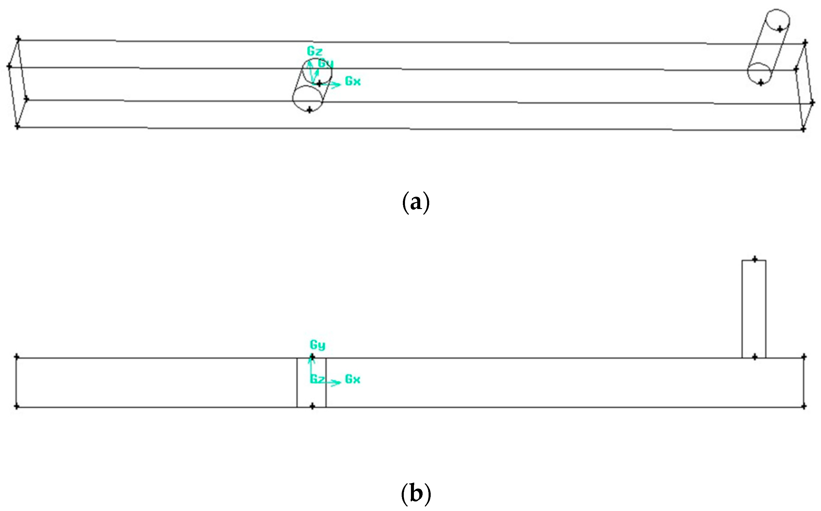
3.3. Meshing and Boundary Conditions

The domain was meshed into structural meshes with 2.0 million cells. The grid size ranged from 0.5 mm to 2 mm, and the near-wall regions were further refined by adaptation. To check the grid independence, the results from three grid schemes were compared with each other. Figure 3 shows the velocity profiles of Re = 12,400 at x = 100 mm downstream simulated based on the standard k-ε closures and the LES approach with the WALE SGS model with three different grid schemes. The grid scheme with 2 million cells was found to be sufficient for both k-ε and LES simulations. The inlet boundary condition was set to a uniform velocity, with three corresponding inlet velocities of 0.176, 0.332, and 0.437 m/s. The turbulence intensity was estimated to be 2% for the inlet. The outlet was set as a pressure outlet and the other boundaries were set as no-slip wall boundaries.

3.4. Solver Settings

ANSYS Fluent was adopted as the solver for the simulations, and a pressure-based transient solver was used. In the present study, the LES approach with SGS models, including the Smagorinsky–Lilly (S-L), WALE, and DKE models, as well as the RANS approach with the standard, RNG and realizable k-ε, and standard and SST k-ω closures, was used for comparisons. The near-wall modeling approach was chosen for LES, and the log-law wall function was chosen for the k-ε closures and k-ω closures. The time step was adjusted using the Courant–Friedrichs–Lewy condition [33] so that the Courant number was less than one. The convergence criteria for the continuity, velocities, and k values were all set to 10−6.
To determine the necessary duration for time averaging of the LES simulation results, the velocity profiles at x = 100 mm obtained from various time durations are compared in Figure 4, where the results were obtained from the LES (results were time-averaged from t = 0 to the specific time) and standard k − ε closure predictions (results were extracted at the specific time). Even though the RANS model solved the flow in a Reynolds averaged manner, the sufficient simulation time still needed to be determined to avoid the effect of the initial condition. From the comparison of different time durations, the simulation time of 15 s was found to be fully sufficient for RANS predictions, and the duration of 25 s was sufficient for LES.

4. Results and Discussion

The mean velocity characteristics at the center plane were obtained from various turbulence closures and were compared with the present experimental data. The velocity profiles along the vertical direction (z axis) were first extracted from the center plane (y = 0) at various streamwise locations (x axis), including x = −75 mm, 50 mm, 75 mm, 100 mm, and 125 mm. The effect of the Reynolds numbers could be assessed by comparing the velocity profiles at the same streamwise location under various Reynolds numbers. The longitudinal velocity profiles along the centerline (y = z = 0) from x = −75 mm to x = 300 mm were also extracted to investigate the velocity variation along the centerline in this section.

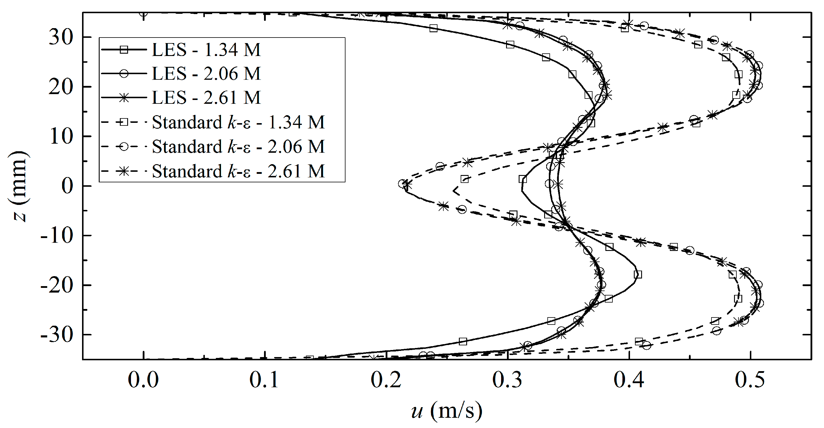
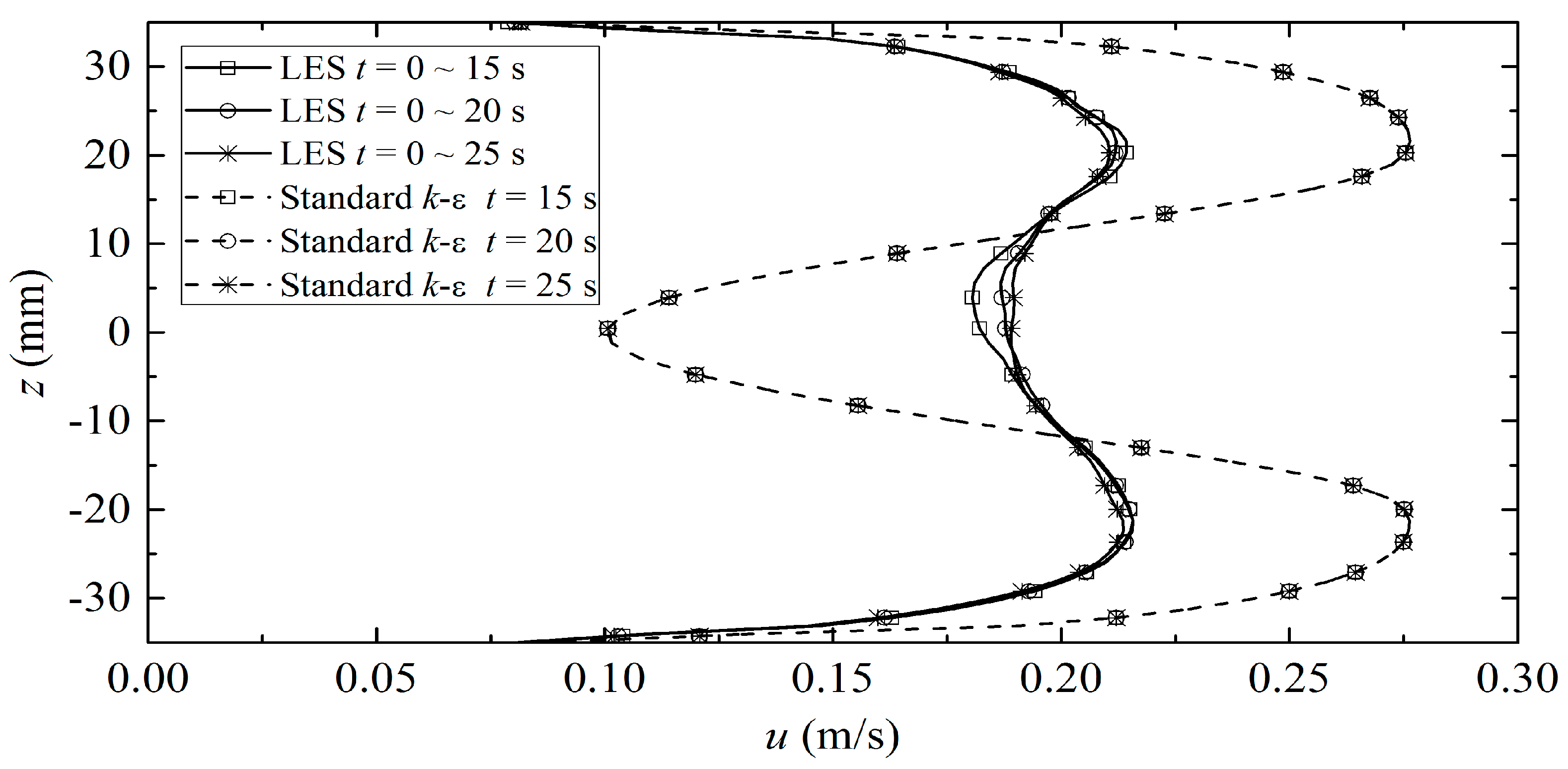
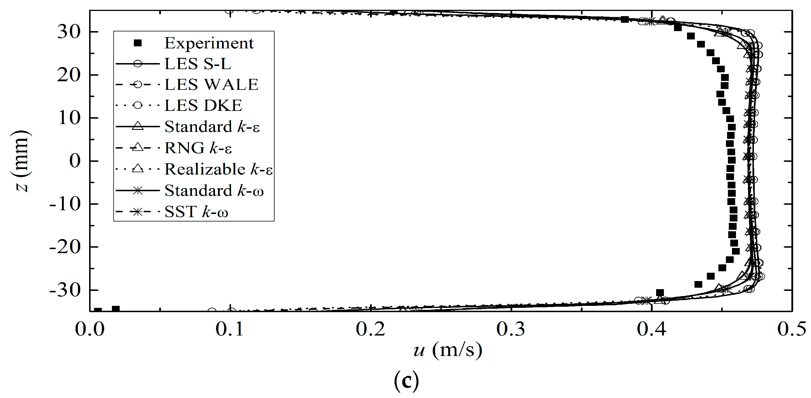
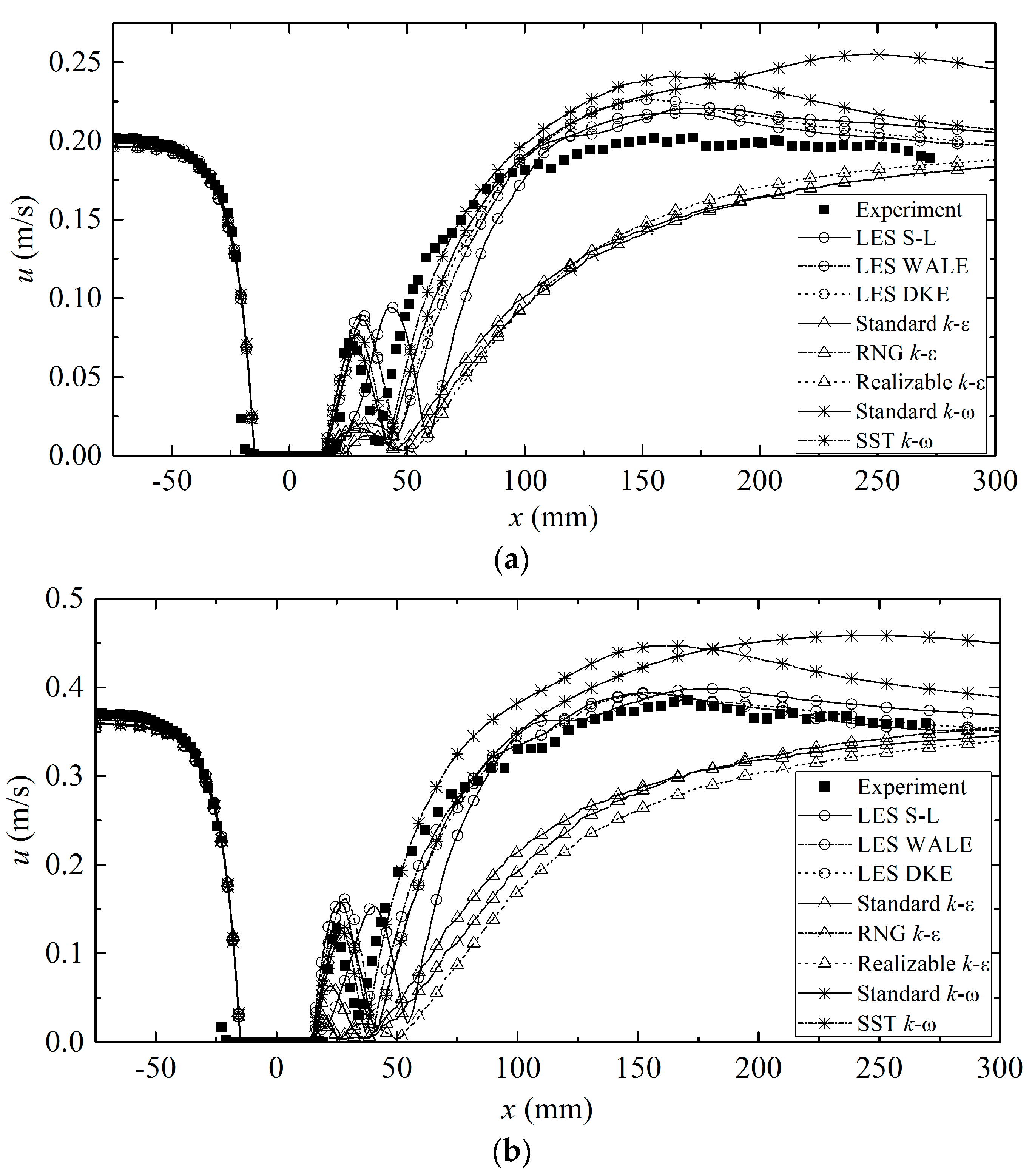
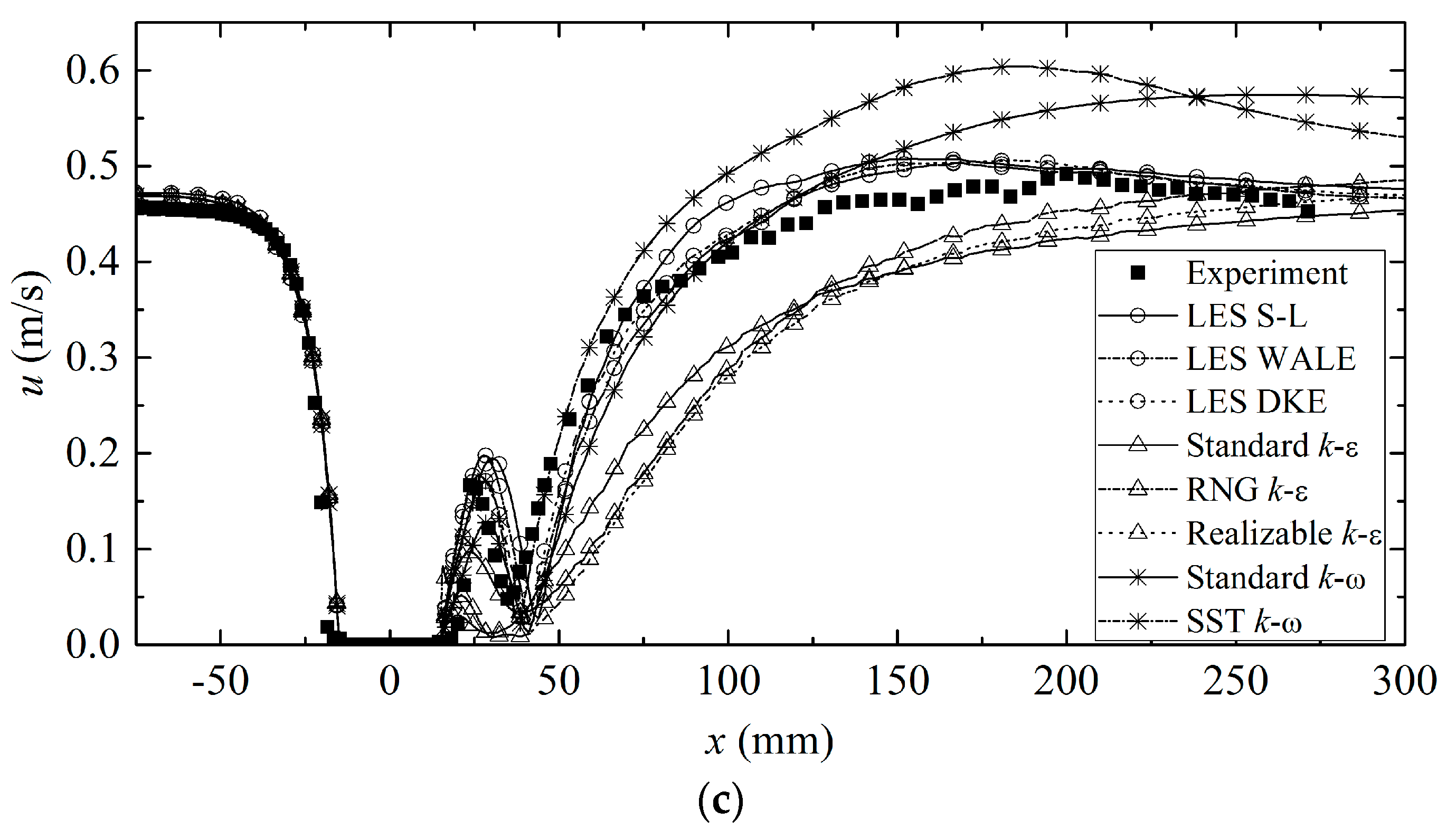
4.1. Velocity Profiles in Upstream Region

It is critical to examine the steady flow profile in the upstream section before the cylinder. Figure 5 shows the vertical velocity profiles in the upstream at x = −75 mm with the three Reynolds numbers. From the experimental data, it can be observed that the velocity profile was slightly more uniform for higher Reynolds numbers. This suggests that the flow field might not be fully developed at the lowest Re, and it was probably due to the insufficient upstream length.
Despite the experimental imperfection, all the numerical results obtained from the different approaches collapsed into a single curve and were somewhat close to the experimental data, revealing the similar performance of these approaches in the prediction of steady upstream flow. A slight difference in the velocities at the centerline between the experimental data and the predicted results can be observed at the highest Re, with the variation around 2%, which was within the experimental uncertainty.

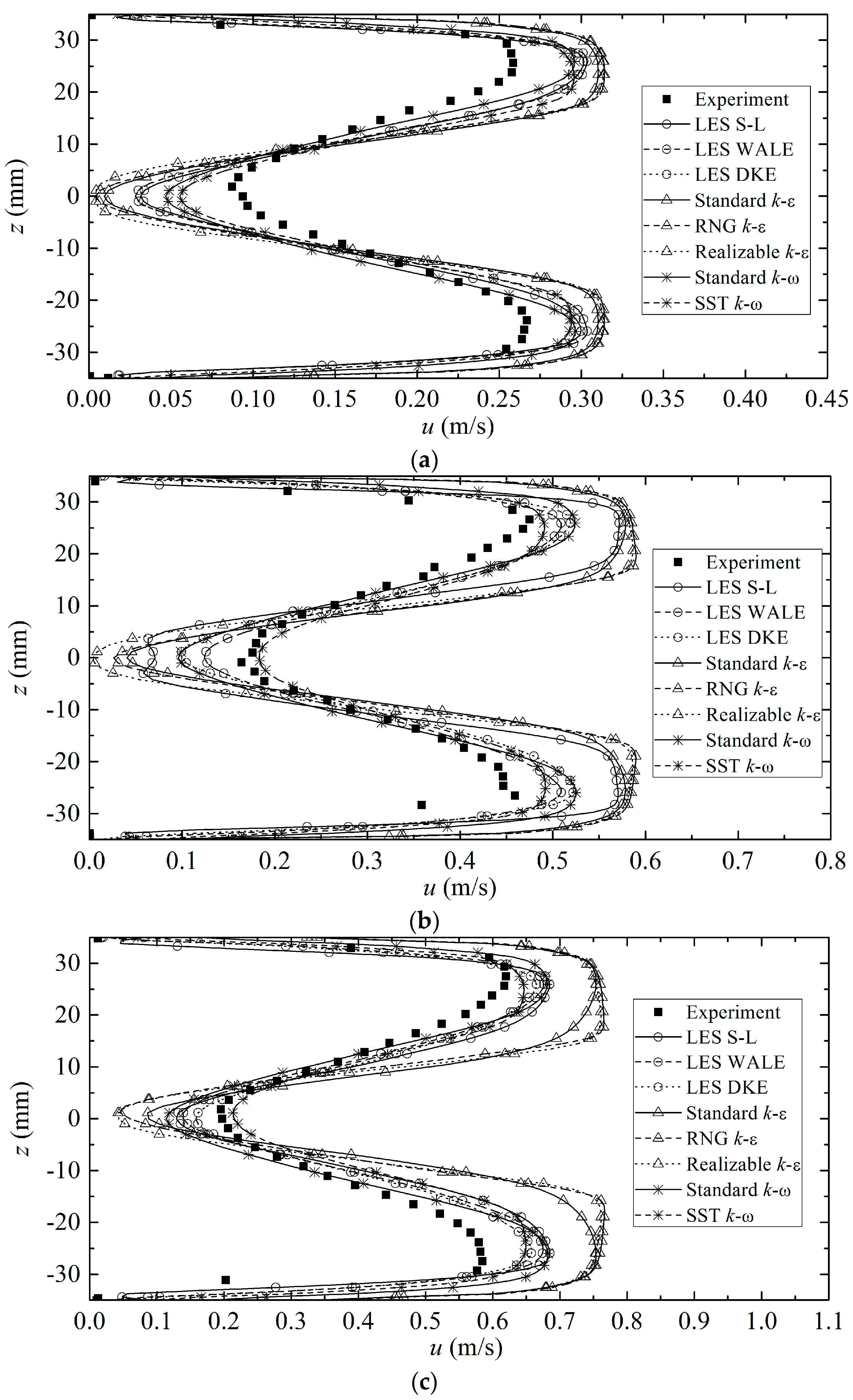
4.2. Velocity Profiles in Wake Region

It was concluded from Figure 5 that the different approaches all provided reasonably good predictions of the steady flow profile in the upstream section. However, behind the cylinder, there existed a wake region in which velocity fields were significantly affected by the cylinder, and the performance of conventional RANS closures was reported to yield poor accuracy [7] in this region. Therefore, the characteristics of the flow in the wake region behind the cylinder required further investigation. In this section, the mean velocity profiles were extracted from various turbulence closures as well as experimental results at different streamwise locations for comparison.
Figure 6 shows a comparison of the velocity profiles at x = 50 mm obtained from the various CFD approaches and experimental observations. From the figure, the velocity profile featured two peaks and one trough, with a local minimum along the centerline. The two peaks were due to flow acceleration with the presence of walls both at the top and bottom where the velocity decreased to zero. The presence of a trough located at the centerline in the wake region was consistent with previous studies [34,35] when the flow passed a cylinder. From the figure, both LES and RANS models with a k-ω closure were found to yield better agreement with the experiments, while RANS with a k-ε closure yielded much higher peaks and lower local minimum values. In terms of the trough, LES produced better predictions with a higher Re.
Further downstream, the velocity profiles at x = 75 mm were extracted and are plotted in Figure 7, in which the curves also generally had two peaks and one trough. Compared with Figure 6, the differences between the extreme values (peaks and troughs) became smaller, indicating the effect of the cylinder was weakened. From the figure, RANS with the three different k-ε closures still far over-predicted the peak values and under-predicted the minimum values. RANS with the three different k-ω closures gave much better predictions of the minimum values but over-predicted the peak values. In comparison, LES, especially the DKE and WALE SGS models, showed its capability of simulating both extreme values reasonably well.
Figure 8 shows the velocity profiles at x = 100 mm. Compared with Figure 6 and Figure 7, the flow profile tended to be much more uniform. In general, RANS models with k-ε closures were unable to reproduce this trend. Among the k-ω closures, the standard k-ω closure better predicted the minimum values at the centerline, but both the standard and SST k-ω closures over-predicted the peaks. In comparison, the LES predictions were consistent with the experimental results. Within LES, the WALE and DKE SGS models were found to be better than the S-L model, which tended to yield more uniform results at large and medium Re values.
In summary, RANS models with k-ε closures were not able to reproduce velocity variations in the wake region, and the k-ω closures provided better predictions but over-predicted the peaks when the flow went downstream from the cylinder. In general, LES, especially the WALE and DKE SGS models, provided the closest results to the experimental data in the wake region.

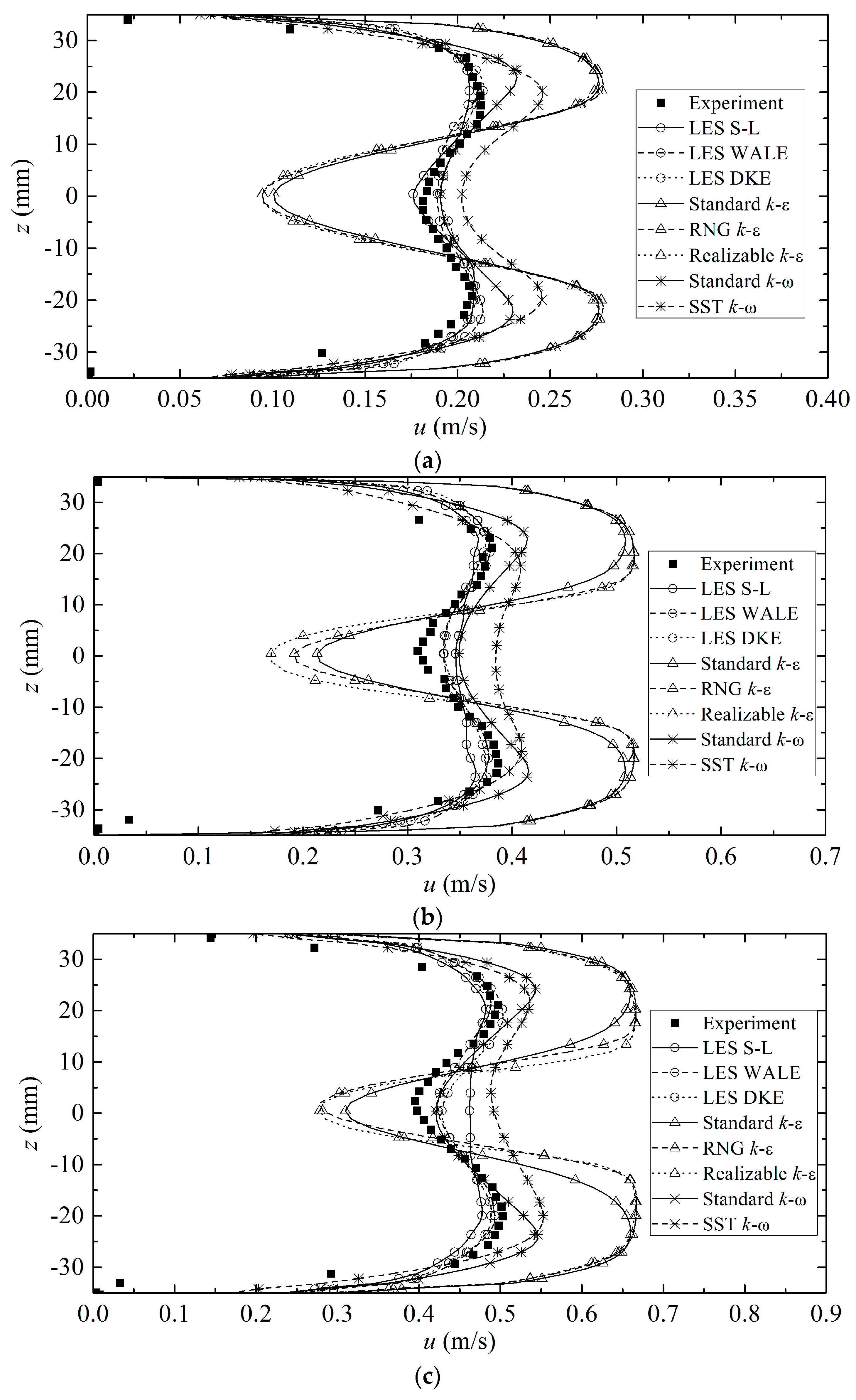
4.3. Velocity Profiles beyond Wake Region

With increasing distance from the cylinder to the downstream, the effect of the cylinder eventually disappeared, and the velocity profiles became uniform in general. Figure 9 shows the velocity profiles at x = 125 mm, and from the figure, the velocity became almost uniform, proving that the influence of the wake region can be negligible at this point.
From the figure, it can be observed that RANS models with k-ε closures were not able to simulate this transition and they tended to predict a much larger wake region. The k-ω closures generally captured this transition better, even though the standard k-ω closure tended to reproduce large wake regions at high Re values. However, both the standard and SST k-ω closures predicted much higher velocities compared with the experimental data. In comparison, LES was able to capture this transition well and the predicted velocities were closer to those in the experimental data. Among all the LES models, the LES S-L model was the best performer.

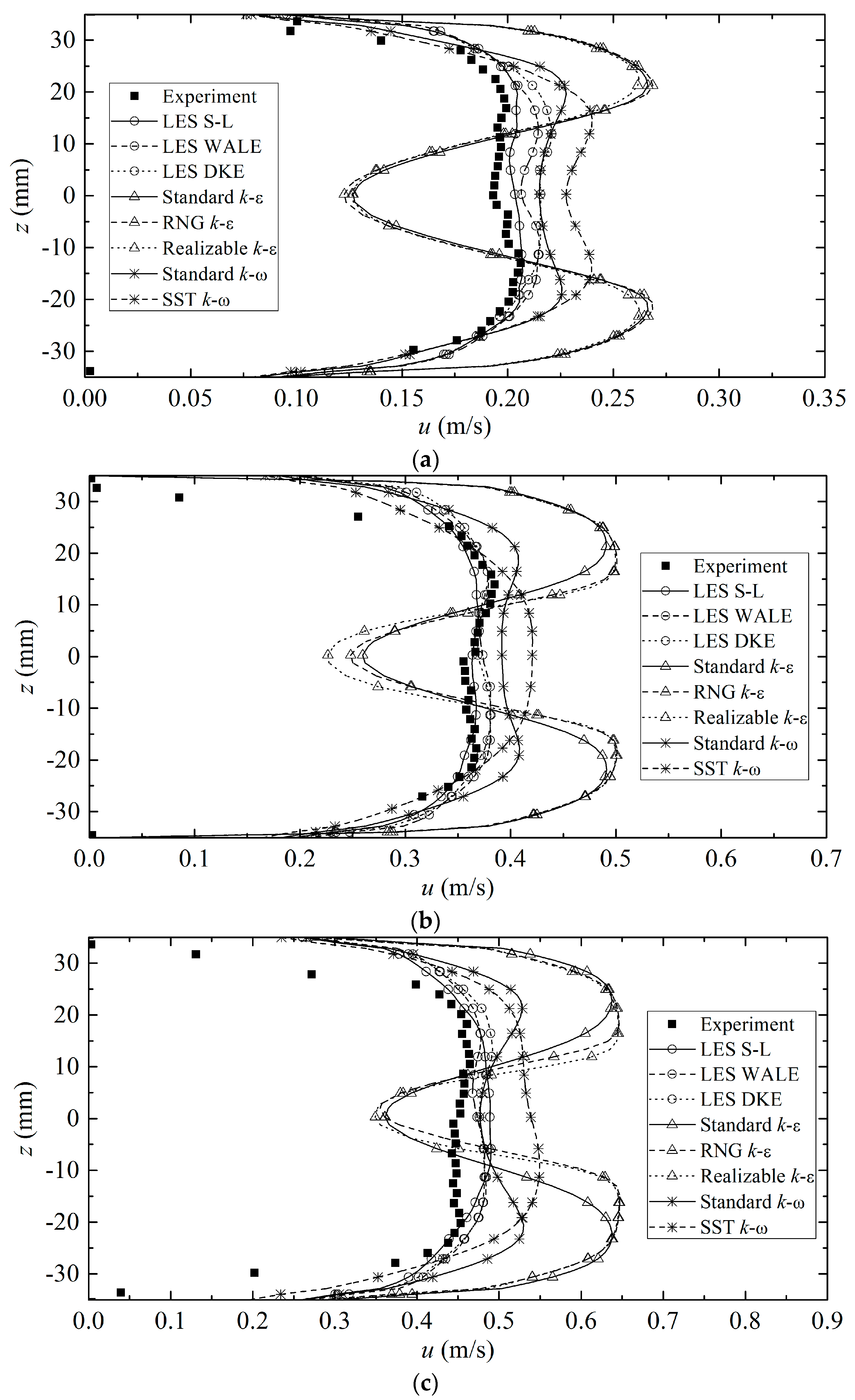
4.4. Longitudinal Velocity Profiles at Centerline

To better understand the flow characteristics, the magnitude of streamwise velocity along the centerline of the reactor was plotted from x = −75 to 300 mm, as shown in Figure 10. It was found that the centerline velocity started to drop from x = −50 mm until reaching zero at the surface of the cylinder. Once the flow passed the cylinder, the velocity increased from zero to a local peak, then decreased again to a local minimum located at around x = 42 mm and seemed invariant with Re. The minimum location was the location where the direction of streamwise velocity changed from negative to positive [35]. Beyond that, the velocity began to positively increase until reaching a steady state.

4.5. Discussion

The better performance of the LES model than any of the RANS models shown in the present study was anticipated and could be explained by the superior theory of LES to RANS. In turbulent flows, the transports of mass, momentum, energy, and other quantities are mainly affected by large eddies which are strongly determined by the boundary conditions, and thus are anisotropic [28]. On the contrary, small eddies are isotropic or tend to be isotropic and are rarely affected by boundaries. In the two types of RANS models, namely the k-ε-type and k-ω-type models, the Boussinesq hypothesis is adopted, which assumes that Reynolds stresses can be incorporated through turbulent viscosity or eddy viscosity (expressed by Equation (3)), to solve Navier–Stokes equations. The underlying assumption of the Boussinesq hypothesis is that the turbulent viscosity is assumed to be isotropic, which may not be true for large eddies, and would therefore lead to false results, which was revealed in the present study.
In contrast, eddies in LES are filtered into large and small parts based on the local grid sizes, and LES models resolve Navier–Stokes equations by computing the relatively large eddies using direct numerical simulation without any hypotheses and simulating the small eddies using appropriate assumptions, namely the SGS models. LES is a workable alternative because previous observation reveals that the scale of eddies ranges from the macro-scale to the micron-scale and most of the energy is contained in the large eddies [36]. Therefore, by direct simulations of large eddies, LES is expected to yield better predictions of the flow than RANS closures. For small eddies, the SGS models can give reasonable results even with relatively coarse grids.
In the present study, among the RANS closures, the k-ω closures yielded better predictions than the k-ε closures in the wake region. This phenomenon can be attributed to the better ability of k-ω closures, by substituting the dissipation rate in k-ε closures with the specific dissipation rate (in Appendix B.1 and Appendix B.2), in coping with the adverse pressure gradients, wall boundary layers, and shear flows [37,38] which exist in the wake region behind the cylindrical sleeve (UV lamp). However, such an ability of k-ω closures adversely becomes a weakness in the far field beyond the wake region, as shown in Figure 10. It is worth noting that SST yielded better predictions than the standard k-ω closure in the far field region, due to its combination of the standard k-ω in the near-wall region and the k-ε closure in the far field [39].

5. Conclusions

The hydrodynamics of the flow passing a cylinder within a closed conduit was investigated by both RANS and LES approaches with various turbulence closures and LES SGS models, respectively. Overall, RANS models with k-ε closures yielded the least accurate results with far under-estimations of the longitudinal velocity in the wake region, while the k-ω closures were in satisfactory agreement with the experimental data near to the cylinder but continuously over-predicted in the far field; LES provided the best fit with the experimental data. Overall, the results illustrated that LES is a better approach than RANS in predicting the flow field around complex boundaries, including possible flow separation, and is thus more suitable for flow field predictions within a UV reactor. In view of the need for reliable predictions of the flow field and inactivation, LES with suitable SGS models is therefore recommended for UV reactors with intensive wall interactions. It is recommended that the LES approach for both the mean flow and Reynolds stress distributions, integrated with a fluence rate model for UV light intensity and a kinetic model for microbial inactivation, should be further evaluated in the future for the design of UV disinfection reactors.

Author Contributions

Conceptualization, A.W.-K.L. and S.Z.; methodology, A.W.-K.L. and S.Z.; investigation, S.Z.; resources, S.Z.; data curation, S.Z.; writing—original draft preparation, S.Z.; writing—review and editing, S.Z and A.W.-K.L.; supervision, A.W.-K.L. All authors have read and agreed to the published version of the manuscript.

Funding

This research received no external funding.

Data Availability Statement

All data were published in the main text.

Conflicts of Interest

The authors declare no conflicts of interest.

Appendix A

Appendix A.1. Standard k-ε Closure

In the standard k-ε closure, the flow is assumed to be fully turbulent and the molecular viscosity is neglected. The turbulent kinetic energy and its dissipation rate can be computed from the following equations [40]:
t ρ k + x i ρ k u i = x j μ + μ t σ k k x j + G k + G b ρ ε Y M + S k
t ρ ε + x i ρ ε u i = x j μ + μ t σ ε ε x j + C 1 ε ε k G k + C 3 ε G b C 2 ε ρ ε 2 k + S ε
where G k = ρ u i u j ¯ u j x i is the generation of the turbulent kinetic energy due to the mean velocity gradients; G b = 1 ρ ρ T g i μ t T P r t x i is the generation of the turbulent kinetic energy due to buoyancy; Y M = 2 ρ ε k a 2 2 is the contribution of fluctuating dilatation in the compressible turbulence to the dissipation rate, where a is the sound speed and S k and S ε are user-defined source terms; and σ k and σ ε are the turbulent Prandtl numbers for k and ε, respectively.
After the turbulent kinematic energy and its dissipation rate are obtained, the turbulent viscosity can be calculated by
μ t = ρ C μ k 2 ε

Appendix A.2. RNG k-ε Closure

Based on the standard k-ε closure, two other closures (RNG and realizable k-ε closures) were developed to improve the performance. The RNG k-ε closure was developed from the standard k-ε closure with refinements based on the renormalization group theory [41].
The transport equations of the RNG k-ε closure are similar to those of the standard closure:
t ρ k + x i ρ k u i = x j α k μ e f f k x j + G k + G b ρ ε Y M + S k
t ρ ε + x i ρ ε u i = x j α ε μ e f f ε x j + C 1 ε ε k G k + C 3 ε G b C 2 ε ρ ε 2 k R ε + S ε
where α k and α ε are the inverse effective Prandtl numbers, and μ e f f is the effective viscosity calculated by RNG theory, which calculates the turbulent viscosity as
d ρ 2 k ε μ = 1.72 μ e f f μ μ e f f μ 3 1 + C v d μ e f f μ
The R ε term is calculated by
R ε = C μ ρ S k ε 3 1 S k ε η 0 1 + β S k ε 3 ε 3 k
where η 0 and β are constants. Using Equation (A7), the ε Equation (A5) can be rewritten as
t ρ ε + x i ρ ε u i = x j α ε μ e f f ε x j + C 1 ε ε k G k + C 3 ε G b C 2 ε ρ ε 2 k
where C 2 ε is computed by
C 2 ε = C 2 ε + C μ ρ S k ε 3 1 S k ε η 0 1 + β S k ε 3
The value of C 2 ε varies with S , which represents the strain rate. When S = 0 , C 2 ε = C 2 ε , which is consistent with the standard closure. Therefore, the RNG closure is more sensitive to the effects of the strain rate.

Appendix A.3. Realizable k-ε Closure

The realizable k-ε closure differs from the standard k-ε closure by two additional modifications: an alternative formulation for the turbulent viscosity, and a modified transport equation for ε . The term “realizable” means that certain mathematical constraints need to be satisfied on the Reynolds stresses, which is consistent with the physics of the turbulent flows. The limitation of the realizable k-ε closure is that, for the computational domain containing both stationary fluid zones and rotating zones, it can produce non-physical turbulent viscosities.
The transport equations with the realizable k-ε closure can be written as follows [42]:
t ρ k + x i ρ k u i = x i μ + μ t σ k k x i + G k + G b ρ ε Y M + S k
t ρ ε + x i ρ ε u i = x i μ + μ t σ ε ε x i + ρ C 1 S ε ρ C 2 ε 2 k + ν ε + C 1 ε ε k C 3 ε G b + S ε
Similar to other k-ε closures, the turbulent viscosity is calculated using Equation (A3). Here, C μ is no longer a constant. Instead, it is calculated by
C μ = 1 A 0 + A s k U ε
where
U S i j S i j + Ω ~ i j Ω ~ i j

Appendix B

Appendix B.1. Standard k-ω Closure

The standard k-ω closure is an empirical closure based on transport equations for the turbulent kinetic energy and specific dissipation rate, ω , instead of the dissipation rate. The turbulent kinetic energy and the specific dissipation rate can be calculated by [38]
t ρ k + x i ρ k u i = x j Γ k k x j + G k Y k + S k
t ρ ω + x i ρ ω u i = x j Γ ω ω x j + G ω Y ω + S ω
where G k = ρ u i u j ¯ u j x i is the generation of the turbulent kinetic energy by the averaged velocity gradients; G ω = α ω k G k is the generation of the specific dissipation rate; Y k = ρ β f β k ω and Y ω = ρ β f β ω 2 are the dissipation of the turbulent kinematic energy and specific dissipation rate, respectively; Γ k = μ + μ t σ k and Γ ω = μ + μ t σ ω are effective diffusivities for the turbulent kinetic energy and specific dissipation rate, respectively; and S k and S ω are source terms.
After solving the transport equations, the turbulent viscosity can be expressed as
μ t = α ρ k ω
where α is the low Reynolds number correction, given by
a = a a 0 + R e t / R k 1 + R e t / R k
where R e t = ρ k μ ω , R k = 6 , and a 0 = 0.024 . When the Reynolds number increases, R e t increases accordingly and, finally, a = a = 1 .

Appendix B.2. SST k-ω Closure

The Shear-stress transport (SST) k-ω closure was developed by combining the formulation of the k-ω closure in the near-wall region with the k-ε closure in the far field, which hereby was converted into the k-ω formulation. Compared to the standard k-ω closure, the SST k-ω closure includes some refinements and is more accurate and reliable for flows including transonic shock waves and adverse pressure gradient flows.
The transport equations for the SST k-ω closure are similar to those for the standard k-ω closure [39]:
t ρ k + x i ρ k u i = x j Γ k k x j + G ^ k Y k + S k
t ρ ω + x i ρ ω u i = x j Γ ω ω x j + G ω Y ω + D ω + S ω
where G ^ k = m i n G k ,   10 ρ β k ω is the generation of turbulent kinetic energy due to the mean velocity gradients; G ω = ω k G ^ k is the generation of the specific dissipation rate; Y k = ρ β k ω and Y ω = ρ β f β ω 2 are the dissipation of the turbulent kinematic energy and specific dissipation rate, respectively, due to the turbulence; D ω = 2 1 F 1 ρ 1 ω σ ω , 2 k x j ω x j is the cross-diffusion term; and S k and S ω are source terms.
The turbulent viscosity is obtained by
μ t = ρ k ω 1 m a x 1 α , S F 2 a 1 ω
where S is the strain rate magnitude, and F2 is the blended function.

Appendix C

Appendix C.1. Smagorinsky SGS Model

The Smagorinsky SGS model was originally developed by [31] for the closure of SGS viscosity. Later, [32] further developed the model, and thus the model is also called the Smagorinsky–Lilly SGS model. The sub-grid-scale turbulent viscosity is modeled in the Smagorinsky SGS model as follows:
μ t = ρ L S 2 S ~
where S ~   2 S ~ i j S ~ i j and L S are the mixing length, given by
L S = m i n κ d w a l l , C S ,
where κ is the Von Karman constant, d w a l l is the distance to the wall, is the grid scale, and C S is the Smagorinsky constant, which usually ranges from 0.1 to 0.2. However, C S may not be a universal constant, thus limiting the prediction capability.

Appendix C.2. Dynamic Kinetic Energy SGS Model

In the Dynamic Kinetic Energy (DKE) model, the transport of the SGS turbulent kinetic energy is defined by [43]
k s g s = 1 2 u k 2 ¯ u ¯ k 2
which is obtained by solving the following transport equation:
ρ k ¯ s g s t + ρ u ¯ j k ¯ s g s x j = τ i j u ¯ i x j C ε ρ k s g s 3 / 2 f + x j ( μ t k ¯ s g s σ k x j )
where the constant σ k is equal to one and the constant C ε is determined dynamically.
The sub-grid-scale turbulent viscosity is thus computed by
μ t = C k ρ k s g s 1 / 2 f
where C k is a constant which is determined dynamically, and f is the filter size that can be computed by
f V 1 / 3
where V is the volume of the computational cell. The SGS stress is thus different and can be written as
τ i j 2 3 ρ k s g s δ i j = 2 μ t C k ρ k s g s 1 / 2 f S ¯ i j

Appendix C.3. Wall-Adapting Local Eddy-Viscosity SGS Model

In the Wall-Adapting Local Eddy-Viscosity (WALE) model, the sub-grid-scale turbulent viscosity is modeled as [44]
μ t = ρ L S 2 S i j d S i j d 3 / 2 S ¯ i j d S ¯ i j d 5 / 2 + S i j d S i j d 5 / 4
where L s and S i j d are computed by
L s = m i n κ d , C w V 1 / 3
S i j d = 1 2 g ¯ i j 2 + g ¯ j i 2 1 3 δ i j g ¯ k k 2 , g ¯ i j = u ¯ i x j
where C w = 0.325 .

References

  1. Hijnen, W.A.M.; Beerendonk, E.F.; Medema, G.J. Inactivation credit of UV radiation for viruses, bacteria and protozoan (oo)cysts in water: A review. Water Res. 2006, 40, 3–22. [Google Scholar] [CrossRef]
  2. Blatchley, E.R. Numerical modelling of UV intensity: Application to collimated-beam reactors and continuous-flow systems. Water Res. 1997, 31, 2205–2218. [Google Scholar] [CrossRef]
  3. Bolton, J.R. Calculation of ultraviolet fluence rate distributions in an annular reactor: Significance of refraction and reflection. Water Res. 2000, 34, 3315–3324. [Google Scholar] [CrossRef]
  4. Ducoste, J.J.; Liu, D.; Linden, K. Alternative Approaches to Modeling Fluence Distribution and Microbial Inactivation in Ultraviolet Reactors: Lagrangian versus Eulerian. J. Environ. Eng. 2005, 131, 1393–1403. [Google Scholar] [CrossRef]
  5. Simons, R.; Gabbai, U.E.; Moram, M.A. Optical fluence modelling for ultraviolet light emitting diode-based water treatment systems. Water Res. 2014, 66, 338–349. [Google Scholar] [CrossRef]
  6. Downey, D.; Giles, D.K.; Delwiche, M.J. Finite element analysis of particle and liquid flow through an ultraviolet reactor. Comput. Electron. Agric. 1998, 21, 81–105. [Google Scholar] [CrossRef]
  7. Liu, D.; Wu, C.; Linden, K.; Ducoste, J. Numerical simulation of UV disinfection reactors: Evaluation of alternative turbulence models. Appl. Math. Model. 2007, 31, 1753–1769. [Google Scholar] [CrossRef]
  8. Lyn, D.A.; Chiu, K.; Blatchley, E.R., III. Numerical Modeling of Flow and Disinfection in UV Disinfection Channels. J. Environ. Eng. 1999, 125, 17–26. [Google Scholar] [CrossRef]
  9. Wols, B.A.; Shao, L.; Uijttewaal, W.S.J.; Hofman, J.A.M.H.; Rietveld, L.C.; Van Dijk, J.C. Evaluation of experimental techniques to validate numerical computations of the hydraulics inside a UV bench-scale reactor. Chem. Eng. Sci. 2010, 65, 4491–4502. [Google Scholar] [CrossRef]
  10. Chiu, K.p.; Lyn, D.A.; Savoye, P.; Blatchley, E.R., III. Effect of UV system modifications on disinfection performance. J. Environ. Eng. 1999, 125, 459–469. [Google Scholar] [CrossRef]
  11. Jenny, R.M.; Jasper, M.N.; Simmons, O.D.; Shatalov, M.; Ducoste, J.J. Heuristic optimization of a continuous flow point-of-use UV-LED disinfection reactor using computational fluid dynamics. Water Res. 2015, 83, 310–318. [Google Scholar] [CrossRef] [PubMed]
  12. Li, H.Y.; Osman, H.; Kang, C.W.; Ba, T. Numerical and experimental investigation of UV disinfection for water treatment. Appl. Therm. Eng. 2017, 111, 280–291. [Google Scholar] [CrossRef]
  13. Munoz, A.; Craik, S.; Kresta, S. Computational fluid dynamics for predicting performance of ultraviolet disinfection–sensitivity to particle tracking inputs. J. Environ. Eng. Sci. 2007, 6, 285–301. [Google Scholar] [CrossRef]
  14. Younis, B.A.; Mahoney, L.; Palomo, N. A Novel System for Water Disinfection with UV Radiation. Water 2018, 10, 1275. [Google Scholar] [CrossRef]
  15. Wols, B.A.; Uijttewaal, W.S.J.; Hofman, J.A.M.H.; Rietveld, L.C.; Van Dijk, J.C. The weaknesses of a k-ε model compared to a large-eddy simulation for the prediction of UV dose distributions and disinfection. Chem. Eng. J. 2010, 162, 528–536. [Google Scholar] [CrossRef]
  16. Zhang, J.; Tejada-Martínez, A.E.; Zhang, Q. Developments in computational fluid dynamics-based modeling for disinfection technologies over the last two decades: A review. Environ. Model. Softw. 2014, 58, 71–85. [Google Scholar] [CrossRef]
  17. Shah, J.; Židonis, A.; Aggidis, G. State of the art of UV water treatment technologies and hydraulic design optimisation using computational modelling. J. Water Process Eng. 2021, 41, 102099. [Google Scholar] [CrossRef]
  18. Cao, H.; Deng, B.; Hong, J.; Xue, J.; Chang, F. Numerical Simulation of the Arrangement of Baffles on Radiation Distribution and Disinfection in UV Reactors. Chem. Eng. Technol. 2016, 39, 108–114. [Google Scholar] [CrossRef]
  19. Chen, J.; Deng, B.; Kim, C.N. Computational fluid dynamics (CFD) modeling of UV disinfection in a closed-conduit reactor. Chem. Eng. Sci. 2011, 66, 4983–4990. [Google Scholar] [CrossRef]
  20. Jenny, R.M.; Simmons, O.D.; Shatalov, M.; Ducoste, J.J. Modeling a continuous flow ultraviolet Light Emitting Diode reactor using computational fluid dynamics. Chem. Eng. Sci. 2014, 116, 524–535. [Google Scholar] [CrossRef]
  21. Kooshan, A.S.; Jalali, A.; Chini, S.F. Performance evaluation of point-of-use UVC-LED water disinfection photoreactors using CFD and response surface methodology. J. Water Process Eng. 2022, 46, 102545. [Google Scholar] [CrossRef]
  22. Li, W.; Li, M.; Bolton, J.R.; Qu, J.; Qiang, Z. Impact of inner-wall reflection on UV reactor performance as evaluated by using computational fluid dynamics: The role of diffuse reflection. Water Res. 2017, 109, 382–388. [Google Scholar] [CrossRef]
  23. Li, H.Y.; Osman, H.; Kang, C.W.; Ba, T.; Lou, J. Numerical and experimental studies of water disinfection in UV reactors. Water Sci. Technol. 2019, 80, 1456–1465. [Google Scholar] [CrossRef] [PubMed]
  24. Bose, R.; Yeo, D. Simulations of Flow over an Axisymmetric Hill; 2021:NIST TN 2141; National Institute of Standards and Technology (U.S.): Gaithersburg, MD, USA, 2021. [CrossRef]
  25. Law, A.W.K.; Wang, H. Measurement of mixing processes with combined digital particle image velocimetry and planar laser induced fluorescence. Exp. Therm. Fluid Sci. 2000, 22, 213–229. [Google Scholar] [CrossRef]
  26. Zhang, S.; Jiang, B.; Law, A.W.K.; Zhao, B. Large eddy simulations of 45° inclined dense jets. Environ Fluid Mech. 2016, 16, 101–121. [Google Scholar] [CrossRef]
  27. Williamson, C.H.K. Vortex Dynamics in the Cylinder Wake. Annu. Rev. Fluid Mech. 1996, 28, 477–539. [Google Scholar] [CrossRef]
  28. Pope, S.B. Turbulent Flows; Cambridge University Press: Cambridge, UK, 2000; Available online: https://pope.mae.cornell.edu/TurbulentFlows.html (accessed on 5 June 2023).
  29. Versteeg, H.K.; Malalasekera, W. An Introduction to Computational Fluid Dynamics: The Finite Volume Method, 2nd ed.; Pearson Education Ltd.: London, UK, 2007. [Google Scholar]
  30. Launder, B.; Spalding, D.B. The Numerical Computation of Turbulent Flow Computer Methods. Comput. Methods Appl. Mech. Eng. 1974, 3, 269–289. [Google Scholar] [CrossRef]
  31. Smagorinsky, J. General Circulation Experiments with the Primitive Equations: I. the Basic Experiment. Mon. Weather. Rev. 1963, 91, 99–164. [Google Scholar] [CrossRef]
  32. Lilly, D.K. The Representation of Small-Scale Turbulence in Numerical Simulation Experiments. 1967, pp. 195–210. Available online: https://opensky.ucar.edu/islandora/object/manuscripts:861 (accessed on 10 January 2024).
  33. Courant, R.; Friedrichs, K.; Lewy, H. On the Partial Difference Equations of Mathematical Physics. IBM J. Res. Dev. 1967, 11, 215–234. [Google Scholar] [CrossRef]
  34. Breuer, M. A challenging test case for large eddy simulation: High Reynolds number circular cylinder flow. Int. J. Heat Fluid Flow 2000, 21, 648–654. [Google Scholar] [CrossRef]
  35. Cantwell, B.; Coles, D. An experimental study of entrainment and transport in the turbulent near wake of a circular cylinder. J. Fluid Mech. 1983, 136, 321–374. [Google Scholar] [CrossRef]
  36. Kolmogorov, A.N. The Local Structure of Turbulence in Incompressible Viscous Fluid for Very Large Reynolds Numbers. Proc. Math. Phys. Sci. 1991, 434, 9–13. [Google Scholar]
  37. Wilcox, D.C. Reassessment of the scale-determining equation for advanced turbulence models. AIAA J. 1988, 26, 1299–1310. [Google Scholar] [CrossRef]
  38. Wilcox, D.C. Turbulence Modeling for CFD; DCW Industries: La Canada, CA, USA, 1998; Volume 2. [Google Scholar]
  39. Menter, F.R. Two-equation eddy-viscosity turbulence models for engineering applications. AIAA J. 1994, 32, 1598–1605. [Google Scholar] [CrossRef]
  40. Launder, B.E.; Spalding, D.B. Lectures in Mathematical Models of Turbulence; Academic Press: Cambridge, MA, USA, 1972. [Google Scholar]
  41. Yakhot, V.; Orszag, S.A.; Thangam, S.; Gatski, T.B.; Speziale, C.G. Development of turbulence models for shear flows by a double expansion technique. Phys. Fluids A Fluid Dyn. 1992, 4, 1510–1520. [Google Scholar] [CrossRef]
  42. Shih, T.H.; Liou, W.W.; Shabbir, A.; Yang, Z.; Zhu, J. A new k-ϵ eddy viscosity model for high reynolds number turbulent flows. Comput. Fluids 1995, 24, 227–238. [Google Scholar] [CrossRef]
  43. Kim, W.W.; Menon, S. Application of the localized dynamic subgrid-scale model to turbulent wall-bounded flows. In 35th Aerospace Sciences Meeting and Exhibit; Aerospace Sciences Meetings; American Institute of Aeronautics and Astronautics: Reston, VA, USA, 1997. [Google Scholar] [CrossRef]
  44. Nicoud, F.; Ducros, F. Subgrid-Scale Stress Modelling Based on the Square of the Velocity Gradient Tensor. Flow Turbul. Combust. 1999, 62, 183–200. [Google Scholar] [CrossRef]
Figure 1. Lab-scale UV reactor (unit in mm): (a) three-dimensional view and (b) top view.
Water 16 00271 g001
Figure 2. Model geometry: (a) overview and (b) top view.
Water 16 00271 g002
Figure 3. Velocity profiles of Re = 12,400 at x = 100 mm.
Water 16 00271 g003
Figure 4. Velocity profile of Re = 6600 at x = 100 mm.
Water 16 00271 g004
Figure 5. Velocity profiles at x = −75 mm: Re = (a) 6600, (b) 12,400, and (c) 16,400.
Water 16 00271 g005aWater 16 00271 g005b
Figure 6. Velocity profiles at x = 50 mm: Re = (a) 6600, (b) 12,400, and (c) 16,400.
Water 16 00271 g006
Figure 7. Velocity profiles at x = 75 mm: Re = (a) 6600, (b) 12,400, and (c) 16,400.
Water 16 00271 g007
Figure 8. Velocity profiles at x = 100 mm: Re = (a) 6600, (b) 12,400, and (c) 16,400.
Water 16 00271 g008
Figure 9. Velocity profiles at x = 125 mm: Re = (a) 6600, (b) 12,400, and (c) 16,400.
Water 16 00271 g009
Figure 10. Longitudinal variation in velocity at the centerline: Re = (a) 6600, (b) 12,400, and (c) 16,400.
Water 16 00271 g010aWater 16 00271 g010b
Table 1. Flow conditions of experiments.
Cases123
Flow Rate Q0 (L/s)0.631.181.55
Cross-Sectional Averaged Velocity U0 (m/s)0.1760.3320.437
Re660012,40016,400
Disclaimer/Publisher’s Note: The statements, opinions and data contained in all publications are solely those of the individual author(s) and contributor(s) and not of MDPI and/or the editor(s). MDPI and/or the editor(s) disclaim responsibility for any injury to people or property resulting from any ideas, methods, instructions or products referred to in the content.

