Abstract
Human migration triggered by flooding will create sociodemographic, economic, and cultural challenges in coastal communities, and adaptation to these challenges will primarily occur at the municipal level. However, existing migration models at larger spatial scales do not necessarily capture relevant social responses to flooding at the local and municipal levels. Furthermore, projecting migration dynamics into the future becomes difficult due to uncertainties in human–environment interactions, particularly when historic observations are used for model calibration. This study proposes a stochastic agent-based model (ABM) designed for the long-term projection of municipal-scale migration due to repeated flood events. A baseline model is demonstrated initially, capable of using stochastic bottom-up decision rules to replicate county-level population. This approach is then combined with physical flood-exposure data to simulate how population projections diverge under different flooding assumptions. The methodology is applied to a study area comprising 16 counties in coastal Virginia and Maryland, U.S., and include rural areas which are often overlooked in adaptation research. The results show that incorporating flood impacts results in divergent population growth patterns in both urban and rural locations, demonstrating potential municipal-level migration response to coastal flooding.
1. Introduction
Changing precipitation patterns, droughts, land degradation, flood events, and sea-level rise already affect many coastal socio-ecological systems (SES). These and other potential climate change impacts on human systems can drive complex, uncertain changes to the population size, resource use, and economic activity of future societies [1], and in some cases, exacerbate human migration patterns [2,3,4,5,6,7]. The fact that climate-induced migration can itself cause subsequent environmental consequences such as deforestation and degradation of natural resources implies the bidirectional relationship between environment and migration [8]. Accordingly, predicting human migration and understanding how relocation dynamics will be influenced by different environmental changes is crucial for both adaptation planning and environmental conservation, as an important input in the decision-making process of many governments and organizations. The United Nations Framework Convention on Climate Change (UNFCCC) has already brought up discussions on the compensation problems for the areas where residents are possibly forced to migrate, such as small-island states confronted by rising sea levels [9].
In response to these challenges, there is a growing body of research on climate-influenced migration that can generally be categorized into three approaches: theoretical frameworks, empirical methods, and agent-based modeling (ABM). Early migration theories were based on economic reasoning (e.g., employment opportunities and income) as the main driver triggering the migration processes [10]. It is also conceptualized using a pull–push model accounting for aspects that attract and repel people to move [11]. This foundation led to further studies that consider other drivers of migration such as environmental, social, political, and demographic forces [12,13,14,15]. Empirical approaches typically use statistical methods to quantitatively identify relationships between environmental change and migration, emphasizing the role of climatic event type and migration characteristics [16,17,18,19,20,21,22,23]. However, empirical approaches require large volumes of data to identify causal relationships, which limits their applicability in contexts with sparse data. While useful to characterize factors influencing migration on a large-scale population level, such methods cannot capture complex granular factors that influence migration decisions at the individual or household level [24]. Finally, empirical analyses of migration behavior can only assess historically observed relationships, which are not necessarily reflective of future migration patterns. For instance, Hauer [25] assumes that migrations happen only among locations that have already experienced migrations historically. However, research that integrates future climate change projections suggests that migration patterns will not necessarily keep up with historically observed patterns [26]. Finally, empirical methods do not capture heterogeneous decision making and behaviors across large populations and only find general patterns and relationships out of collective data.
Agent-based modeling (ABM) provides an alternative mechanism to represent heterogeneous decision-making processes and human responses to natural disasters where individual-level variation in behaviors leads to emergent collective outcomes, such as evacuation [27,28,29,30] and migration [31,32]. Numeric simulations of multi-agent systems can capture effects stemming from heterogeneity across different types of actors [33]. ABM can allow social, economic, and environmental factors to be incorporated into a migration model that considers social-ecological feedbacks, evolutionary learning, and out-of-equilibrium dynamics to better capture complex system characteristics of migration patterns due to climate change [34]. These factors can be combined with spatial data to develop a spatially explicit simulation of climatic risks and associated individual responses. The latter is important as SES often shows high levels of spatial variability. Through spatial ABMs, possible interactions between social systems and spatially explicit environmental systems (such as the dynamics of sea-level rise and inundated areas across spatial scale) can be better tracked. The added value of ABM is its ability to explore dynamic paths of SES, which usually involve abrupt changes and transitions emerging from cumulative effects of social interactions and adaptive behaviors, since other modeling approaches that assume perfect information and static or rational behavior may be misleading [35].
ABM has been recently used to study migration in response to different environmental factors, including studies that assess different theoretical foundations [36] and incorporate temporal dimensions [37,38,39]. One key challenge in ABM in any context is model validation [40], with multiple studies calling for more systematic and rigorous model validation processes [35,41]. Forward-looking ABMs which consider sea-level rise as one of the environmental drivers in their model [31,32] usually validate simulations only by feeding historical data to the initialization step. However, developing and validating forward-looking models using historical data may not produce valid projections of migration into the future. The lack of calibration to compare model results in forward-looking ABMs can affect the credibility of their long-term migration projections in the context of climate change.
Existing empirical models of climate-induced migration primarily focus on livelihood-based migration at international or national scales [42,43]. Spatially explicit ABM can complement this work by tracking displacements for more detailed regional assessment and planning. For instance, Hassani-Mahmooei and Parris [31] investigate internal migration across all divisions of Bangladesh using a temporal-spatial ABM. Models of migration decision making over smaller scales (municipal to regional) can be beneficial in addressing multiple issues. First, national-scale findings are not necessarily representative of the specific migration drivers and their impacts on regional and municipal scales. This is particularly important in adaptation planning, as many actions in response to SLR and flooding (such as infrastructure hardening or zoning changes) are taken by local governments or regional agencies. Local mobility in response to climate stressors could have significant implications for municipalities, for instance, by exacerbating population loss in rural communities or intensifying urban housing shortages. While national-scale studies mostly consider migration from a livelihood perspective (for example, subsistence farmers who must migrate when crop yields decline), many other factors combine to influence human spatial behavior and vary among regions and social groups [44]. At smaller spatial scales, people’s displacements occur across shorter distances which may not lead to different jobs or wages. Thus, the factors that drive people to move at local scales may be quite different than at large scales and include factors such as housing, family, and educational opportunities [45]. Existing ABMs of local mobility responses to sea-level rise or flooding typically adopt an economic focus on housing market dynamics based on utility maximization [32,46,47,48]. However, this does not account for other factors that influence relocation decision making, such as disaster impacts on infrastructure and community services [49]. Finally, a quick comparison between the portion of rural versus urban governance structures which do have adaptation and land-use planning sections (31% versus 71%) shows that rural settings are usually overlooked in adaptation research [50]. At the same time, they are often even more vulnerable to climate impacts due to factors such as demography, occupations, earnings, literacy, poverty incidence, and dependency on government funds [51]. A small spatial scale can allow distinguishing between urban and rural settings and their unique characteristics, compare their migration response, and investigate outcomes on their municipal structure.
To address the aforementioned gaps, this study proposes a stochastic ABM for flood-induced migration at the municipal to regional level across rural and urban coastal areas. This ABM is based on the push–pull theory of migration which posits that the decision to migrate stems from numerous factors driving people away from certain locations and attracting them to others [52,53,54]. A set of bottom-up agent-level decision rules is calibrated to replicate county-level population projections from NASA’s Socioeconomic Data and Applications Center (SEDAC). This step provides a baseline model of population movement in the study region and demonstrates that individual decision rules can be formulated to replicate macro-scale behavior in best-available population projects. This model is then used to assess the impact on census tract-level population distribution under different assumptions about the relative role of flooding in individual migration decisions under multiple 50-year storylines of nuisance and extreme flooding. This model is then utilized to determine how flooding alters the spatial and temporal patterns of population change relative to baseline projections that do not consider flooding. This general approach can provide a foundation for further investigations on flood-induced migration based on available public data that can be expanded to accommodate various decision rules and projections of coastal flood risk.
2. Materials and Methods
The proposed method revolves around the concept of simulating migration behavior in response to flooding through a bottom-up mindset using ABM. In an ABM, a system is depicted as a group of independent decision-making entities known as agents. Each agent autonomously evaluates its circumstances and makes decisions based on a predefined set of rules. These agents may engage in a set of actions based on the interactions defined in the system they represent. ABM captures the emergent behavior arising from the interplay of individual entities within their environment. Emerging phenomena such as flood-induced human migration as a whole exceed the mere sum of its parts due to the inherent dynamics of this system.
This research developed a stochastic ABM based on the push–pull migration theory for flood-induced migration across flood-prone rural and urban areas of coastal Virginia and Maryland. Initially, a baseline model was developed and calibrated to simulate individual agent migration decisions as a stochastic process, relying on the underlying pull score of the census tract in which they currently live, without considering flood impacts. This model was then used to simulate migration patterns under different storm surge flood storylines derived from the U.S. Army Corps of Engineers’ North Atlantic Coast Comprehensive Study storm surge hazard assessment [55] and under different sea-level rise scenarios. Migration simulations were conducted with different assumptions about the importance of storm surge flooding relative to other factors that influence migration decisions and evaluated the degree to which storm surge flooding causes future projections to deviate from our baseline model (Figure 1). Model simulations were run for a 50-year simulation period from 2021 to 2070, to assess how repeated and aggregated individual relocation decisions impact municipal-scale population patterns in flood-prone areas over the long term.
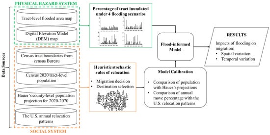
Figure 1.
Schematic overview of proposed ABM.
2.1. Study Area
The study area considered in this research comprises 16 coastal counties within the states of Virginia and Maryland, U.S. This study location includes both urban and rural coastal areas with both increasing and decreasing population over the past decade (Figure 2). Sea levels have risen significantly faster in the Mid-Atlantic U.S. region compared to the global average due to land subsidence from sediment compaction, glacial isostatic rebound, groundwater extraction, and weakening Gulf Stream currents, making this area the second largest population center at SLR-related risks in the U.S. [56,57,58,59]. The rate of SLR in coastal Virginia is predicted to increase 13.1% to 71% by 2100 [60], which is exacerbated due to the low-lying topography in this area [61]. Higher sea level increases the extent of flooding even without the occurrence of rainfall. Even though sea levels have only risen by around 12.7 cm, the annual frequency of minor flooding events has increased by 33% in some areas of Virginia since 2000 [62]. While rarely damaging, minor flooding can lead to notable disruptions affecting quality of life, such as school closures, infrastructure shutdowns, and difficulty accessing community services. Sea-level rise also increases the risks and potential impacts from larger flood events in the region, including tropical storms and hurricanes. The annual accelerating frequencies and cumulative effects of floods are becoming a threatening problem in several locations with strategic importance to national security, including Norfolk, Virginia [62].
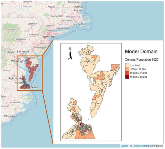
Figure 2.
The model domain delineated by U.S. census tracts and colored by the real population in 2020 [63].
2.2. Baseline Model
The goal of the baseline model was to develop a set of stochastic agent decision rules that could effectively replicate broad-scale population projections in the study area. For this purpose, best-available dataset of county-level population projections based on SSPs [64,65] was utilized. These top-bottom data-driven projections were obtained from transforming county-level historic U.S. census data to cohort-change ratios (CCRs) and cohort-change differences (CCDs), projecting CCDs and CCRs using Autoregressive Integrated Moving Average (ARIMA) models, and feeding them to Leslie matrix population projection models, subject to SSPs’ control to avoid runaway population growth. A key advantage of the statistical approach used to generate these projections is the explicit ability to account for statistical error terms and quantify uncertainty in future projections. Consequently, incorporating these details into agent-based modeling simulations would be a valuable area of additional research.
In an ABM, agents can individually assess their situation and take actions based on a set of decision rules [66], which can aggregate into emergent phenomena where group-level behavior differs from the individuals alone. The factors that influence population growth and decline in urban and rural areas are highly complex, including proximity to employment opportunities and wages [67], housing prices [68], and public services such as taxes, education, unemployment insurance benefits, and public safety [69]. Explicitly simulating all of these factors is beyond the scope of this work. As an alternative, our baseline model combined a “pull score” that describes the relative desirability of each census tract based on population growth projections.
U.S. Census tracts were used as the spatial unit within the model, allowing for the integration of physical flood inundation data in later steps. The forward-looking simulation is conducted yearly so that each time step represents a year from 2021 to 2070. Each agent in the model represents a group of 200 individuals, which serves as a representative sample of the real population in the study area. The abstraction level of 200 individuals per agent was made to balance computational efficiency and statistical representation, aligning with prior research that successfully aggregated agents to simulate the climate-induced migration behavior of extensive populations [31]. As the stochastic nature of the model required running multiple simulations to determine system behavior under each scenario, aggregating individuals into groups allows capturing the inherent heterogeneity within the population while reducing computational complexity. This value results in an initial population of 2602 agents in 2021, representing a study area population of 520,400 individuals. In each time step, agents are randomly assigned a satisfaction score based on the push–pull score of the census tract in which they currently live; these push–pull scores are derived from county-level population projections [64,65]. The current model uses the satisfaction score as an aggregate measure summarizing the numerous factors that influence an individual’s desire and capability to relocate, such as economic reasons and job opportunities, information concerning alternative localities, demographic characteristics such as age, education level, and parenthood, and psychic cost of migration [70]. Because of the challenges inherent in measuring and simulating these factors explicitly at the individual scale, a stochastic approach is adopted that samples a random satisfaction value across a known distribution, with the acknowledgment that individuals will vary in their satisfaction in ways that are impossible to predict.
NetLogo [71] is used as the modeling toolkit which is a programmable environment for simulating natural and social phenomena. The overview of the modeling approach is shown in Figure 3. The model is initiated through a setup phase, where the spatial features of the model are integrated into the NetLogo environment, push–pull factors for each census tract are calculated, and agents are generated across the study area. For each year of the simulation, a two-phase process is used to simulate agent moves within the study area (blue box in Figure 3), and agent moves in and out of the study area (red box in Figure 3). The details of each step of the model process are discussed in more detail in the following sections.
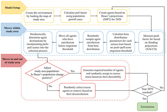
Figure 3.
The flowchart overview of the agent-based mode.
2.2.1. Data Sources
Census tract-level data and geographic boundaries within the study area [63] were used to define the spatial setting of the model. For the baseline model, push–pull scores for each census tract were defined based on population projections to 2070. A common critique of model-based projections of future conditions, including but not limited to ABMs, is that calibrating models using historical data inherently assumes that future events and consequences will follow historical trends. This is unlikely to be the case in situations with the multi-dimensional uncertainties and complexities inherent to socio-environmental systems. To address this issue, county-level population projections [64,65] for the study region were used to develop and calibrate the baseline model. These projections were created by developing autoregressive models of projected rates of population change based on observed data from 1960–2016 [64,65]. These projections do not explicitly consider potential environmental influences that could impact population changes in a given area, such as sea-level rise. Thus, these are used as baseline projections for how the population would likely evolve if flooding impacts are not considered, and then this baseline is used as a comparison for different flood scenarios.
Projections from the Shared Socioeconomic Pathway SSP2 were used to calculate an annual linear growth rate. These projections, representing population trends at the county level, were then disaggregated into census tracts within each county based on their respective 2020 population (Figure 4). While linear population trends will not be applicable in all cases, a comprehensive analysis using least squares regression of the 2020–2070 projections demonstrated that in all but one county in the study area, at least 74% of the projection could be explained by a linear trend. To convert the county-level growth rates to the individual census, the county growth rate was used as the mean of a normal distribution from which census tract growth rates were sampled, with higher-populated tracts receiving higher percentile values. This process facilitated an effective distribution of the county-level population projections to the census tract level, accounting for variations in population size and growth patterns within and across counties.
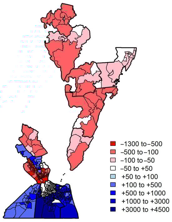
Figure 4.
Annual population growth rates for the census tracts of the study area.
2.2.2. Individuals’ Behavior and Decision Making
In this model, the approach taken for the agents to make migration decisions is associated with two groups of factors, including (1) push factors that encourage an agent to leave their current location (e.g., lower inherent desirability or larger area percentage flooded), and (2) pull factors that determine where agents relocate to. Agents will evaluate their current location based on pull–push factors to decide if they prefer to migrate. Then, they evaluate other locations again based on pull–push factors to decide where to move. To account for the numerous factors not explicitly represented in the model, a stochastic approach is employed where agents’ satisfaction is randomly sampled based on a beta distribution with parameters that vary depending on the push–pull score of the agents’ location. A summary of the model parameters and state variables used to represent agent behavior are presented in Table 1 and described in more detail in the following sections.

Table 1.
State variables and global model parameters.
Push–pull scores for each census tract were calculated based on linear rates of population growth or decline. Rates of census tract population change G, which ranged from −1300 to 4500 persons per year in the study area, were translated into a pull score P for each census tract i ranging between 0 and 1 using a logistic function governed by a parameter, (Equation (1)). The logistic function allows transforming the growth rates into a [0, 1] bounded probability scale, while the use of a parameter (Figure S1) allows the process to be replicated in other study areas using the same projection source.
A value of zero results in a uniform distribution and leads to random movement between census tracts regardless of their projected growth rate [65]. Greater values result in greater differences in the pull scores of high and low growth rate tracts. Thus, increasing results in greater migration flows to high-growth tracts.
Within a given census tract, agents will vary in terms of their desire and ability to move based on numerous factors that are difficult to measure, let alone simulate. This inclination to move, referred to as agent satisfaction S, was thus represented using a random variable sampled from a beta distribution, the parameters of which would change based on the pull score P of agent’s location. The beta distribution is confined to the interval (0, 1) and governed by two shape parameters α and β. Agents’ satisfaction scores were modeled using a beta distribution because its interval aligns with the range of pull scores and the distribution offers great flexibility in modeling various shapes of distributions, including symmetrical, skewed, U-shaped, inverted U-shaped, and straight lines (Figure S2). This flexibility was desirable as there was no predetermined assumption about the distribution of satisfaction levels within the study area and we sought to calibrate it with a high level of flexibility. The mean () and variance () of beta distribution are formulated by Equation (2) and Equation (3), respectively:
To calculate a beta distribution for agents within a census tract based on the pull score P, two parameters and υ were defined. The parameter defines the relationship between tract pull score P and the mean of the beta distribution as in Equation (4).
A value of equal to 0 leads to a mean value for the distribution of agent satisfaction regardless of P, meaning that tracts’ pull score has no influence on expected agent satisfaction. As the value of increases, the mean value of the distribution for S will move from 0.5 toward the value of P, resulting in higher satisfaction scores for agents in high pull-score tracts. A value of equal to 1 leads to for tract .
The parameter υ represents the sum of shape parameters α and, β (Equation (5)) and indirectly controls the variance of the beta distributions across each census tract. Higher values of υ lead to lower variance in the distribution of satisfaction S. Thus, a high value of both and υ would result in a high correspondence between census tract pull P and agent satisfaction S, due to low-variance distributions of S centered on different mean values. Figure 5 demonstrates the effect of changing and υ on the distributions used to sample agent satisfaction within low (P = 0.3) and high (P = 0.8) pull-score tracts. For the purposes of this model, υ was constrained to the interval (4, 20). Given a set of model parameters and υ and a census tract pull score P, the beta distribution parameters α and β can be calculated as in Equations (6) and (7):
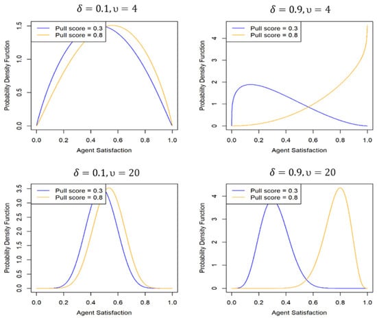
Figure 5.
Examples of how adjusting global model parameters and υ influence the distributions used to sample agent satisfaction in high pull-score tracts and low pull-score tracts.
Since the distribution of satisfaction is unknown and dependent on the study area and perceptions and values of the residing people, this distribution is allowed to have different shapes based on the inherent desirability of a location through parameters and υ, while considering the possibility of its being bell-shaped () as well. Several factors can contribute to the possibility of considering people‘s satisfaction distribution as normally distributed, similar to various other phenomena. The first significant factor is the level of complexity and randomness. In complex systems or processes involving a large number of random variables, the cumulative effect tends to produce a normal distribution. This is because the likelihood of extreme values occurring in multiple variables simultaneously decreases, promoting a bell-shaped curve [72]. Second is the effect of statistical aggregation. Many measurements in science, economics, and social sciences involve the aggregation of numerous small, independent influences. When these influences are combined, the resulting distribution often conforms to the normal pattern.
At each time step of simulating pull–push effects, agents’ satisfaction scores are sampled from the associated distributions. A threshold was considered for migration decisions to be made, with which agents’ satisfaction scores S were compared. If their satisfaction was less than this move threshold , they decided to migrate. Agents’ decisions about their migration destination were based on the pull score P of the tracts, meaning that tracts with higher pull scores are more likely to be migrants’ destinations. Agents did so using NetLogo’s built-in weighted random draw method in destination selection, where the likelihood of a census tract being selected as a destination is directly proportional to that census tract’s pull score. In summary, numeric ranges were established as follows: tract-level G scores in our study area varied from −1300 to 4500. P, S, F, and P* are assigned values within the range of 0 to 1 for standardization purposes. The parameter δ modifies the mean of the satisfaction distribution based on P, resulting in a mean value between 0.5 and P. Additionally, the parameter υ adjusts the sum of shape parameters in the satisfaction distribution, with a specified range (4, 20). This range is selected to account for distribution variances, leading to a diverse array of distribution shapes. MT is a level to which satisfaction score is compared, which is set to values below 0.5 to mitigate excessive migration flows.
2.2.3. Baseline Model Calibration
The global parameters , , υ, and were calibrated by systematically testing all combinations of values for parameters within the bounds presented in Table 1. For each combination of parameter values, the relative root mean square error (Relative RMSE) between the modeled and projected population [64,65] in each simulation year was calculated as in Equation (8).
where is county’s simulated population obtained from the model in year and tract , is county’s projected population projection for the corresponding year and tract, is the total number of census tracts in the study area, and is the number of simulation years.
The ABM model was also evaluated to be consistent with nationwide statistics on local and regional scale mobility developed by the Harvard Joint Center for Housing Studies [45]. Based on this data, 13% of the U.S. population moves each year. Of these moves, 65% are within the same county, and 17% are towards different counties, but in the same state. For the baseline model, the combination of parameter values with the lowest RMSE was selected that also had a movement percentage within 2% of the HJCHS estimate of 10.7%.
2.3. Flood-Informed Model
2.3.1. Physical Flood Inundation Modeling
To represent potential flood events over the period of simulation, statistical coastal flood hazard data were utilized from the U.S. Army Corps of Engineers’ 2015 North Atlantic Coast Comprehensive Study [55,73]. The NACCS statistics represent the combined flood hazards from Nor’easters, tropical storms, and hurricanes and include the influence of astronomical tides. The NACCS statistical values are reported for present-day sea level at return periods (one over annual exceedance probability) ranging from 1 to 10,000 years. The NACCS probabilistic surge hazard methodology is consistent with the methodology now adopted by FEMA for establishing Flood Insurance Rate Maps. The NACCS present-day flood statistics were used to estimate a percentage of each census tract inundated for the floods with return periods of 1, 2, 5, 10, 20, 50, 100, 200, and 500 years. These percentage inundation values were linearly interpolated to yield estimates of inundation percentages for storms with return periods between the nine return periods listed above. This study assumes flooding scenarios under current sea levels as an initial step in demonstrating how flood impacts can be incorporated into a baseline ABM calibrated to long-term projections that do not explicitly consider sea-level rise or other environmental factors. This general approach could accommodate multiple methods for representing future flood scenarios under different assumptions about sea-level rise informed by different data sources. Under different SLR projections, it is expected that the proposed overall approach would not change but that the increasing intensity of floods may intensify migration flows and patterns observed here.
While the NACCS hazard statistics are presented in terms of the return period, the ABM required sequences of flood events through time to simulate the impact that repeated flood events of differing intensities could have on migration behavior. To address this requirement, four 50-year flood storylines were generated representing different long-term scenarios of flood occurrence. To create these storylines, uniform distribution was used to generate 300 sequences of fifty (the number of years in our simulation) random numbers between 0 and 1 and inverted them to obtain sequences of flood return periods. For example, a random number of 0.5 would equate to a two-year flood occurring, whereas a random number of 0.1 would equate to a 10-year flood occurring. Then, a search was conducted across this ensemble of statistically feasible 50-year flood sequences to identify sequences that demonstrated behavior consistent with four conceptual storylines (Figure 6) that represent feasible long-term sequences of flood events in the region:
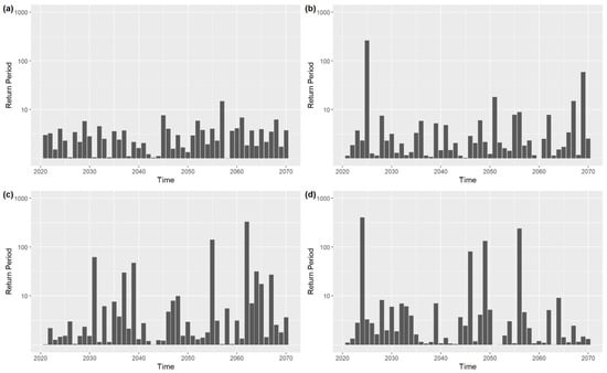
Figure 6.
Conceptual storylines: (a) minor flooding, (b) early severe flooding event, (c) late severe flooding event, (d) two severe flooding events. The values represented in y-axes are log-transformed return periods to better demonstrate the minor flooding events.
- Storyline 1: Frequent small floods (with a return period of 2–10 years).
- Storyline 2: Frequent small floods and one severe storm (with a return period of 100 years or more) occurring early in the horizon (within the first 15 years).
- Storyline 3: Frequent small floods, one large storm (with a return period of 10–100 years), and two severe storms (with a return period of 100 years or more) occurring late in the horizon (within the last 15 years).
- Storyline 4: Frequent nuisance flooding, one large storm (with a return period of 10–100 years), and three severe storms (with a return period of 100 years or more).
Because the time step of the ABM is yearly, these 50-year flood storylines represent a single instance of flooding per year, and thus cannot account for the effect of multiple flood events in a year. While this may underestimate the impact of minor flooding with a return interval of less than one year, as well as the occurrence of multiple large floods in a single year, these details could be incorporated into more sophisticated flood storylines in further work.
2.3.2. Adjustment of Decision Rules
As a simple initial decision rule structure, it was assumed that agents would make decisions about moving from or staying in a census tract using a weighted average of the pull–push score () from the baseline model and the severity of flooding they experience. Flooding severity was represented by the percentage of the census tract that is inundated in a given year (). While the pull–push score is calculated the same as the way it was in the baseline model (Equation (1)), flood-influenced push–pull score for census tract is updated as Equation (9).
The weight represents the relative importance of flooding in comparison with the census tract’s baseline desirability. Different values of were tested to see how the migration response would differ from baseline model projections as flood impacts become an increasing influence on the decision-making process.
is then used to obtain the mean of satisfaction beta distribution and its shape parameters. From this distribution, is calculated for its residing agents to compare with the threshold as in Equations (2)–(7) but calculated as a function of .
It should be mentioned that agents’ decisions about migration destinations are made only based on the pull–push score of destination options. This assumes that agents do not have a detailed awareness of flood impacts or vulnerability in their destination. However, this advancement could be incorporated into our general framework in future research.
2.3.3. Model Simulations and Analysis
Because the model leverages a stochastic approach to modeling agent behavior, 50 simulations were conducted for each weighting scheme, using the mean and standard deviation of which to characterize average population projections under different scenarios and variability stemming from stochastic behavior. The performance of the flood-informed ABM was compared with the baseline model by calculating the deviation of each stochastic iteration under the weight of from the average of stochastic iterations in the baseline scenario. Equation (11) shows baseline population projections against which the flood-informed models were compared:
where N is the number of stochastic iterations, equal to 50. The root mean square of relative deviations from the baseline was then used to characterize spatial and temporal variations:
where is the relative deviation from baseline of stochastic iteration under flood weight of , is the population of stochastic iteration in tract and year under flood weight of , is the number of years simulated (50), and is the total number of census tracts (430).
To measure temporal variability across the study area, the relative deviations were aggregated over all census tracts in each simulated year under each storyline.
where is the annual relative deviation for year under flood weight of from baseline averaged across all census tracts. Additionally, a measure was defined for relative deviation in each census tract in year . This measure was used to show spatial variation of deviation in the study area for a specific year (2070) and flood weight.
is the tract-level relative population deviation for tract from year 2021 through year under flood weight of .
3. Results
3.1. Baseline Model Calibration
The baseline model was calibrated by running 256 simulations in a full factorial arrangement of the four global model parameters (, , υ, and MT) to identify parameter values that best replicated population projections [64,65] and broad-scale movement patterns. The ranges of values tested for each parameter and the final results of calibration are mentioned in Table 2.
Table 2.
Calibration parameters, ranges, and calibrated values.
The comparison between the projected and simulated populations resulted in a minimum relative RMSE of 0.17 in 2070 for the whole study area and an average of 12.6% of agents migrating each year. To ensure that the calibrated ABM was accurately replicating population trajectories, projected and modeled population trajectories were compared for counties with high growth (G > 700 persons per year), moderate growth (0 < G < 700 persons per year) and declining (G < 0 persons per year) populations. This comparison along with a scatter plot of projected versus modeled population across all census tracts and years is presented in Figure 7. While the model reliably replicates population trajectories in the counties experiencing rapid growth (blue lines) and moderate growth (green lines), its performance is poorer in counties experiencing population decline. This is possibly due to the format of the logistic function and its lower bound being set to zero for the push–pull score of negative-growth counties; refining this process would be a valuable area for further research. Despite this limitation, these results indicate that the bottom-up stochastic decision rules of the ABM can reasonably replicate top-down projections from [64].
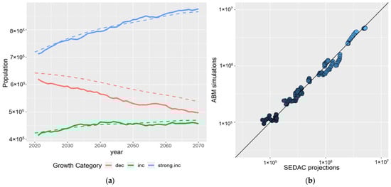
Figure 7.
(a) Study area population simulated by the ABM (solid lines) in comparison with Hauer’s projections (dashed lines) through time. (b) Scatter plot of ABM population simulation results for the study area versus top-bottom population projections [64,65].
3.2. Flood-Informed System Behavior
In order to see how flooding impacts the system behavior given the uncertainty about the relative role of flood impacts in decision making, multiple values of flood weight were simulated and compared with baseline model projections (W = 0). Figure 8 demonstrates the difference between model projections under each flood storyline and the baseline scenario for different values of flood weight. The starting point of all the lines is the same, which is our baseline scenario where the weight of flooding is equal to zero. As the weight applied to the census tract-flooded extent in calculating the push–pull score (Equation (10)) increases, different types of relative divergence from the baseline model emerge from individual-level decision making. Although it is unlikely that high weights of flooding represent realistic preferences, the purpose here is to explore how the system responds under different assumptions about flood importance.
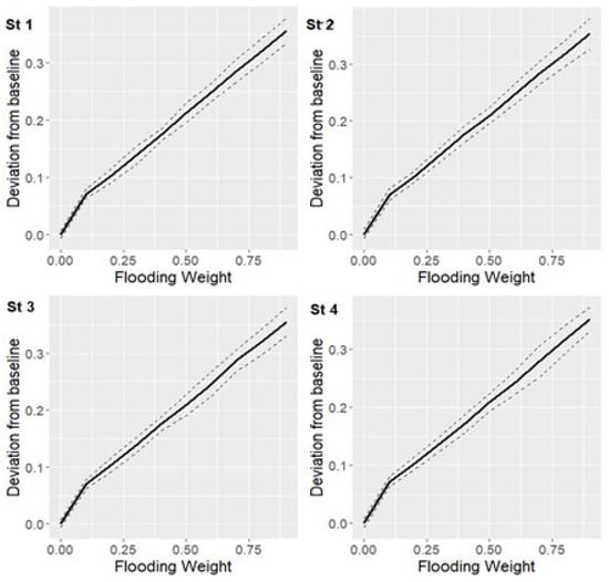
Figure 8.
Relative deviation from baseline scenario under different storylines using different values for the flood weighting factor. The solid line represents the average deviation across the 50 stochastic iterations, and the dashed lines represent the range of deviation across the stochastic iterations to capture the effect of randomness on the model output.
The response under different storylines follows a trend similar to deviation under nuisance flooding of storyline 1, and system behavior shows sensitivity to severe flooding events with subtle bumps. Two severe flooding events in storyline 4 do not show a significant synergic effect. This could potentially be due to the fact that highly vulnerable areas to flooding have already experienced high flows of out-migration when another large flooding event occurs late in the time horizon. It is possible that considering experience memory for agents results in more different behavior under different flood sequences, which needs to be further investigated; however, with the simple assumptions in the decision rules of this model, the system’s migration response to different flood weighting schemes is not highly sensitive to the severity of flooding events.
The relative deviation measures formulated in Equations (13) and (14) only represent the degree to which flood-informed model simulations diverge from the baseline model but do not reveal the direction of population deviations or the specific years or locations where these deviations occur. To spatially characterize flood-induced changes in population projections, Figure 9 presents a tract-level map of relative deviations from baseline to identify areas more prone to in- and out-migration flows. The maps in Figure 9 demonstrate this spatial variation in 2070 under four flood storylines and two different flood weight values. In general, spatial patterns of population deviation were consistent across flooding storylines. The locations that lose population when flood impacts are incorporated, indicated in shades of red, mostly include urban areas. However, the locations that gain population include both urban and rural settings. Comparing migration maps with flood exposure in the study area also reveals that highly inundated areas do not necessarily lose population. Thus, the migration flow cannot be fully explained by urban/rural classifications or flooding alone. In a small number of census tracts, the direction of change relative to baseline projections changes from positive to negative depending on the flood storyline. This demonstrates the complexity of climate migration in the face of multiple intervening factors affecting general migration patterns. The increase in the flooding factor from 0.3 to 0.6 triggers stronger migration flows and more change in population distribution highlighted as relative deviation values from baseline in Figure 9, but the general spatial patterns are consistent.
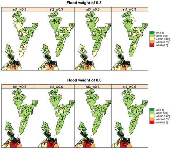
Figure 9.
Spatial variation of relative population deviation from baseline scenario in 2070 under different storylines with flooding weight values of 0.3 and 0.6.
The time series of relative deviation across the study area, illustrated in Figure 10, shows a nonlinear increase through time, which is enhanced under a higher weight of flooding in agent decision making. When the flood weight W equals 0.3, storyline 1 (nuisance flooding with no extreme events) results in a significantly lower deviation from baseline than the storylines that do entail large flood events. However, at higher values of W, the deviation through time in the nuisance flooding storyline is more aligned with the others. In addition, the gradient of change in deviation from baseline in both graphs shows a decreasing trend through time for all storylines. This is notable because large flood events included in storylines 2, 3, and 4 do not result in a significant spike in deviation, and the gradient of change is almost similar over different storylines. This may stem from the fact that all storylines include frequent nuisance flooding that occurs in most years and acts as a chronic, long-term influence on location push–pull scores that outweighs the impact of infrequent large floods. The decreasing gradient of change could indicate that people have already moved from areas highly exposed to flooding to safer locations toward the end of the time horizon. The same time steps ahead do not lead to high out-migration flows anymore as in the past.
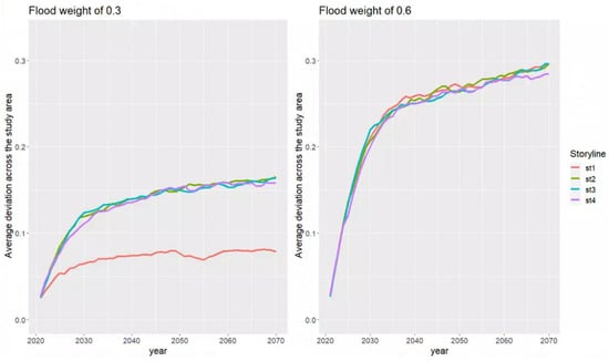
Figure 10.
Temporal variation of relative population deviation from baseline scenario under different storylines with flooding weight values of 0.3 and 0.6. Note that major flood events (>200 years) occur in 2025 in storyline 2, 2062 in storyline 3, and both 2024 and 2056 in storyline 4.
4. Discussion
This study presents a novel stochastic ABM of long-term changes in local-scale migration patterns influenced by repeated coastal flooding. The ABM framework can enrich systems’ understanding and modeling by incorporating bounded rationality, heterogeneity, interactions, evolutionary learning, and out-of-equilibrium dynamics of human behavior in a spatially explicit model [35]. Moreover, bottom-up approaches such as ABM can support a more detailed exploration of micro-level displacement patterns that usually emerge from differing individual decisions, but are masked through behavior generalization approaches commonly extracted from large amounts of data in top-bottom data-driven models.
This research demonstrates that bottom-up individual decision rules can replicate externally derived population projections, providing a baseline for incorporating local-scale factors such as nuisance and extreme flooding. This provides an alternative to models calibrated to historic population changes, and allows an understanding of how flooding could impact future population shifts relative to projections that do not include this hazard. This approach thus complements top-down data-driven models that have been widely applied to investigate migration response to climatic events. Top-down approaches primarily rely on historic patterns for calibration. However, inherent uncertainties, the significant number of interactive subsystems and feedback loops [74] constrain the reliability of model projections. This is particularly true in the case of models that incorporate human behavior, as research has shown that structural decisions in terms of how human behavior is modeled can result in significant uncertainty that greatly exceeds uncertainty stemming from model parameterization and calibration [75]. Accordingly, variable human decision making suggests that good historical performance does not necessarily guarantee future accuracy [76], especially when migration projection is triggered by climate change over a long-term time horizon.
In the face of acknowledged uncertainties, it is helpful to be explicit about what a model (agent-based or otherwise) can and cannot tell us. Aligning with the existing literature, it is asserted that models of highly complex socio-environmental systems are unlikely to be useful as consolidative models that can be used in a predictive sense, as the significant uncertainty and unpredictability in human behavior and its drivers will undermine the reliability of any prediction derived from them [77].
As an alternative, researchers have proposed adopting an exploratory modeling approach that interprets models as computational experiments that reveal system-level outcomes if different assumptions embedded in the model are correct [78]. Adopting this perspective, validating the model against best available population projections based on historical data provides a mechanism for assessing whether bottom-up decision rules can replicate these projections which were derived based on an autoregressive approach. Once this has been confirmed, this serves as a mechanism for experimentally evaluating how the introduction of a new factor (flooding) results in outcomes that diverge from the projections.
The proposed approach also acts as a practical shortcut, circumventing potential uncertainties and intricacies linked to modeling individual population components such as fertility and mortality. This approach is especially beneficial given the frequent challenges associated with obtaining the required data. Another notable aspect of the population projection dataset [64] specifically used in this study is its capacity to offer projections under five socio-economic pathways (SSPs), each contributing to significant variations in geographic growth patterns. Beyond enhancing our comprehension of demographic shifts in small areas of the United States, utilizing this dataset amplifies the method’s adaptability, making it applicable to diverse regions with varying data availability. Additionally, it facilitates the consideration of different SSPs in the planning process, further enriching the method’s overall flexibility.
The increasing encounters with recurrent flooding and recent major coastal disasters are gradually changing attitudes toward relocation among residents and other stakeholders [79]. A survey of coastal residents found that 87% would consider relocating now or in the future due to flooding [80]. Understanding the impact this flood-driven mobility will have on municipalities and their adaptation capacities requires tools that can accurately replicate population-level behavior at fine spatial scales. Moreover, adaptive policy frameworks need to reflect behavioral processes and incentives at the individual, household, community, and organizational levels [81]. Bottom-up approaches that build upon the proposed framework can thus serve as a valuable tool for evaluating and comparing diverse coastal adaptation strategies, of course within the constraints of the modeled representation of coastal community drivers and processes [82]. For instance, by combining the proposed framework with simulations of coastal adaptation, e.g., [83], ABM can facilitate more informed policy-making processes in response to coastal flooding.
The spatial representation and diversity in the environmental context in ABMs are often needed to capture spatial heterogeneity of inputs and outputs. However, existing research mostly chooses the spatial representation based on the available data, without systematically justifying their spatial resolution or extent [35]. In this study, a detailed spatial scale (census tract) was intentionally selected and other data sources were rescaled to this level to discern potential implications of local-scale relocation. Detailed spatial representation allows for the incorporation of small-scale variations in flooding and tracking relocations over short distances, which can be stimulated by different migration purposes represented by stochastic agent behavior. Although census block level as the unit of analysis could provide a more spatially detailed representation of relocation behavior in comparison with census tract, their use over the longer term presents methodological issues: first, census blocks’ boundaries frequently change after the census is conducted each decade based on changes in block population. While this can also occur with census tracts, it happens much less frequently. For instance, while in the study area comprising 16 counties, the initial number of census tracts was 430 according to census 2010; this count increased to 481 in census 2020 due to boundary adjustments. Second, the proposed model was constructed as a framework adaptable for the inclusion of social and economic attributes, most of which are accessible at the census tract level. The census tract level was chosen due to data availability constraints, as several of these variables are not readily accessible at the census block level. Given these challenges, the loss in granularity from using the census tract level does not detract from the objectives of this study, which aims to conceptualize a bottom-up model that integrates population movement at the municipal level in response to flood events. Thus, instead of a high-resolution track of each household’s movement, insights into potential changes in population distribution were gained. This information can be beneficial for the future use of policymakers in flood-prone municipalities, while keeping the required computational effort to apply this framework at a feasible level. Note that the use of census tract spatial scale in previous research on population and policy with ABM [84,85] increases the meaningfulness of this choice of spatial unit for the purpose of informing policy decisions at the municipality scale. Nevertheless, the incorporation of finer-scale spatial processes and data is a potentially valuable area of future research.
This stochastic ABM framework is presented as a first step in modeling individual migration decisions at local scales. As such, a simple representation of human behavior was adopted that could accommodate a more sophisticated representation of migration decision making in many ways. The current framework assumes that migration patterns in the study area follow the estimations provided by HJCHS as well as our suggested heuristic decision rules. Nonetheless, it is worth acknowledging that ABM frequently involves simplifications and assumptions about intricate social and ecological processes, potentially leading to an oversimplification of real-world dynamics and constraining the model’s precision [86]. The structural model choices made regarding the representation of human behavior significantly impact the credibility and validity of modeling insights. Therefore, evaluating the implications of these choices should be regarded as a crucial aspect of future modeling efforts [75]. Primary data collection such as surveys can further complement the ABM model by incorporating additional variables and yielding more robust results [87]. Individual-level details of ABM in the context of climate-related migration decisions could be further advanced by incorporating behavioral psychology and decision theories in the computational modeling of climate migration phenomena. This approach also provides a ground to explore relocation complexities and categories of communities’ response and comparison of the results with previously suggested theoretical classifications such as forced migrants, trapped population, and adaptive migrants [88].
The general framework presented here could also provide a foundation for the testing of different theoretical assumptions in a spatially explicit data-informed manner. For instance, how will migration response vary under sudden and unexpected hazards versus repeated nuisance events, and how does learning from experience and exposure to flood hazards at the individual level influence migration decisions? The proposed approach could also accommodate a more detailed and comprehensive representation of physical hazards. For example, our approach could incorporate an explicit representation of sea-level rise to simulate migration response under different SLR projections, where greater flood intensities could exacerbate the migration flows. Another way to consider a more precise representation of the physical system is to capture heterogeneity in land use within a given census tract. Assuming that high levels of inundation result in a high impact of flooding on residents could result in overestimating the flood impact in areas with low population density but high percent inundated area. An alternative to solve this issue can be updating the model using downscaled population projections, e.g., [89,90] in rural areas to overcome this overestimation. Finally, the proposed ABM approach rests on the assumption that the projections used for the baseline model are a reasonable representation of feasible future conditions. As such, the model can be tested against multiple population projections to account for uncertainty. There is a notable capacity in social system representation as well, which has not yet been of much consideration in population–environment assessments [88].
Ultimately, the modeling framework presented here could help advance the incorporation of coupled social, organizational, biophysical, and hazard systems in stochastic models that include location-specific interactions and feedback loops. Our current study focused on establishing a simple bottom-up framework with a forward-looking calibration step that can serve as a flexible foundation for future research that incorporates additional complexity, such as incorporating interactions among individuals. This enhances the model’s ability to capture the complex interplay between individuals and their environment. In the context of flood-induced migration, the role of social networks, community norms, information sharing, and collective decision making in shaping migration decisions can lead to cascading effects throughout the community. The role of considering interactions extends beyond the social system and also encompasses the interactions between the social and physical hazard systems. For example, one of the main reasons for land subsidence in coastal Virginia and Maryland is groundwater withdrawal. Localities can affect the extent of groundwater extraction, and accordingly, sea-level rise and migration, showing a bidirectional relationship in this area. An additional level of complexity emerges from the intricate interactions and feedback loops between the social system and infrastructure and governance factors. An example is between migration, tax revenues and the protection services provided by municipalities. The modeling approach presented here could serve as a means for incorporating more biophysical, political, and organizational components to yield more comprehensive results.
5. Conclusions
This study presents a stochastic ABM of flood-induced migration flows to simulate the role of individual decisions in relocation outcomes at municipal scales important for coastal adaptation. This approach aims to replicate the behavior of data-driven population projections with stochastic decision-making processes to simulate the impacts of repetitive flooding on a well-validated baseline projection. The proposed method integrates physical flood exposure data with a bottom-up simulated social system and provides detailed population projections in response to repeated flooding for 16 counties in coastal Virginia and Maryland, including both urban and rural settings. The results confirm the ability of ABM to match data-driven approaches even using simple heuristic decision rules. While simple heuristic rules were adopted in this study, the general framework can serve as a foundation for the incorporation of more complex representations of behavior, policy, and physical risk to investigate complex drivers of migration in the context of climate risks. This stochastic agent-based modeling approach can be applied at municipal scales to integrate a wide range of information, observations, and theories into projections that can inform municipal adaptation decision making in the future due to recurrent and extreme flooding. This study suggests multiple directions for future research. These include the implication of modeling choices for the emergent migration patterns, as well as migration response under different theoretical assumptions in different model components. For example, an assessment of the physical hazard system could evaluate the impact of different types of flood scenarios, such as infrequent extremes versus nuisance events and different SLR projections. An evaluation of the social system could include incorporating behavioral psychology, decision theories, individuals’ interactions, and social networks. The impact of human–environment interdependencies would benefit from considering alternative adaptation measures, incorporating primary data, exploring different community-level response categories, and the effect of learning from past experiences being exposed to flooding. Finally, coupling the proposed framework with organizational and biophysical systems could advance methods for systems integration within ABMs.
Supplementary Materials
The following supporting information can be downloaded at: https://www.mdpi.com/article/10.3390/w16020263/s1, Figure S1: Census tract growth rates are mapped to baseline pull scores through a logistic function with parameter; Figure S2: Beta distribution. Shape parameters examples are illustrated. Refs [45,52,53,54,55,64,65,70,73,91] are cited in the Supplementary Files.
Author Contributions
Z.N.: methodology, formal analysis, visualization, writing—original draft preparation; J.E.S.: funding acquisition, conceptualization, methodology, writing—review and editing; A.B.: funding acquisition, conceptualization, data curation, writing—review and editing; Y.S.: data curation, writing—review and editing; J.L.I.: data curation, writing—review and editing. All authors have read and agreed to the published version of the manuscript.
Funding
This research was funded by the US National Science Foundation (NSF), grant number 1920478.
Data Availability Statement
All data and code used in this research are freely accessible online at https://osf.io/6r5ab/?view_only=aab370279b9d4c5bbd44b33238bf25c3, (accessed on 1 January 2024).
Conflicts of Interest
The authors declare no conflict of interest. The funders had no role in the design of this study; in the collection, analyses, or interpretation of data; in the writing of the manuscript; or in the decision to publish the results.
References
- Cairns, G.; Ahmed, I.; Mullett, J.; Wright, G. Scenario method and stakeholder engagement: Critical reflections on a climate change scenarios case study. Technol. Forecast. Soc. Change 2013, 80, 1–10. [Google Scholar] [CrossRef]
- Döös, B.R. Environmental Degradation, Global Food Production, and Risk for Large-Scale Migrations. Ambio 1994, 23, 124–130. [Google Scholar]
- Hugo, G. Environmental Concerns and International Migration. Int. Migr. Rev. 1996, 30, 105–131. [Google Scholar] [CrossRef]
- MacKellar, F.L.; Lutz, W.; McMichael, A.J.; Suhrke, A. Population and Climate Change; Rayner, S., Malone, E.L., Eds.; Battelle Press: Columbus, OH, USA, 1998; Available online: https://iiasa.dev.local/ (accessed on 23 November 2023).
- Magadza, C. Climate Change Impacts and Human Settlements in Africa: Prospects for Adaptation. Environ. Monit. Assess. 2000, 61, 193–205. [Google Scholar] [CrossRef]
- Meze-Hausken, E. Migration caused by climate change: How vulnerable are people in dryland areas? Mitig. Adapt. Strateg. Glob. Change 2000, 5, 379–406. [Google Scholar] [CrossRef]
- Myers, N. Environmental refugees: A growing phenomenon of the 21st century. Philos. Trans. R. Soc. Lond. Ser. B Biol. Sci. 2002, 357, 609–613. [Google Scholar] [CrossRef] [PubMed]
- de Sherbinin, A.; VanWey, L.K.; McSweeney, K.; Aggarwal, R.; Barbieri, A.; Henry, S.; Hunter, L.M.; Twine, W.; Walker, R. Rural household demographics, livelihoods and the environment. Glob. Environ. Change 2008, 18, 38–53. [Google Scholar] [CrossRef]
- Owen-Burge, C. Climate Refugees—The World’s Forgotten Victims [Internet]. Climate Champions. 2021. Available online: https://climatechampions.unfccc.int/climate-refugees-the-worlds-forgotten-victims/ (accessed on 16 January 2023).
- Massey, D.S. A Missing Element in Migration Theories. Migr. Lett. 2015, 12, 279–299. [Google Scholar] [CrossRef]
- Lee, E.S. A theory of migration. Demography 1966, 3, 47–57. [Google Scholar] [CrossRef]
- Black, R.; Adger, W.N.; Arnell, N.W.; Dercon, S.; Geddes, A.; Thomas, D. The effect of environmental change on human migration. Glob. Environ. Change 2011, 21, S3–S11. [Google Scholar] [CrossRef]
- Hunter, L.M.; Luna, J.K.; Norton, R.M. Environmental Dimensions of Migration. Annu. Rev. Sociol. 2015, 41, 377–397. [Google Scholar] [CrossRef] [PubMed]
- McLeman, R.A. Climate and Human Migration: Past Experiences, Future Challenges; Cambridge University Press: Cambridge, UK, 2014; p. 313. [Google Scholar]
- Piguet, E. Linking climate change, environmental degradation, and migration: A methodological overview. WIREs Clim. Change 2010, 1, 517–524. [Google Scholar] [CrossRef]
- Bohra-Mishra, P.; Oppenheimer, M.; Hsiang, S.M. Nonlinear permanent migration response to climatic variations but minimal response to disasters. Proc. Natl. Acad. Sci. USA 2014, 111, 9780–9785. [Google Scholar] [CrossRef] [PubMed]
- Feng, S.; Krueger, A.B.; Oppenheimer, M. Linkages among climate change, crop yields and Mexico–US cross-border migration. Proc. Natl. Acad. Sci. USA 2010, 107, 14257–14262. [Google Scholar] [CrossRef] [PubMed]
- Gray, C.L.; Mueller, V. Natural disasters and population mobility in Bangladesh. Proc. Natl. Acad. Sci. USA 2012, 109, 6000–6005. [Google Scholar] [CrossRef] [PubMed]
- Gray, C.; Wise, E. Country-specific effects of climate variability on human migration. Clim. Change 2016, 135, 555–568. [Google Scholar] [CrossRef]
- Marchiori, L.; Maystadt, J.-F.; Schumacher, I. The impact of weather anomalies on migration in sub-Saharan Africa. J. Environ. Econ. Manag. 2012, 63, 355–374. [Google Scholar] [CrossRef]
- Mastrorillo, M.; Licker, R.; Bohra-Mishra, P.; Fagiolo, G.; Estes, L.D.; Oppenheimer, M. The influence of climate variability on internal migration flows in South Africa. Glob. Environ. Change 2016, 39, 155–169. [Google Scholar] [CrossRef]
- Mueller, V.; Gray, C.; Kosec, K. Heat stress increases long-term human migration in rural Pakistan. Nat. Clim. Change 2014, 4, 182–185. [Google Scholar] [CrossRef]
- Thiede, B.C.; Gray, C.L. Heterogeneous climate effects on human migration in Indonesia. Popul. Environ. 2017, 39, 147–172. [Google Scholar] [CrossRef]
- Kniveton, D.; Smith, C.; Wood, S. Agent-based model simulations of future changes in migration flows for Burkina Faso. Glob. Environ. Change 2011, 21, S34–S40. [Google Scholar] [CrossRef]
- Hauer, M.E. Migration induced by sea-level rise could reshape the US population landscape. Nat. Clim. Change 2017, 7, 321–325. [Google Scholar] [CrossRef]
- Robinson, C.; Dilkina, B.; Moreno-Cruz, J. Modeling migration patterns in the USA under sea level rise. PLoS ONE 2020, 15, e0227436. [Google Scholar] [CrossRef]
- Chen, Y.; Wang, C.; Du, X.; Shen, Y.; Hu, B. An agent-based simulation framework for developing the optimal rescue plan for older adults during the emergency evacuation. Simul. Model. Pract. Theory 2023, 128, 102797. [Google Scholar] [CrossRef]
- Joo, J.; Kim, N.; Wysk, R.A.; Rothrock, L.; Son, Y.-J.; Oh, Y.-G.; Lee, S. Agent-based simulation of affordance-based human behaviors in emergency evacuation. Simul. Model. Pract. Theory 2013, 32, 99–115. [Google Scholar] [CrossRef]
- Lee, S.; Jain, S.; Ginsbach, K.; Son, Y.-J. Dynamic-data-driven agent-based modeling for the prediction of evacuation behavior during hurricanes. Simul. Model. Pract. Theory 2021, 106, 102193. [Google Scholar] [CrossRef]
- Silva, A.F.R.; Eleutério, J.C. Effectiveness of a Dam-Breach Flood Alert in Mitigating Life Losses: A Spatiotemporal Sectorisation Analysis in a High-Density Urban Area in Brazil. Water 2023, 15, 3433. [Google Scholar] [CrossRef]
- Hassani-Mahmooei, B.; Parris, B.W. Climate change and internal migration patterns in Bangladesh: An agent-based model. Environ. Dev. Econ. 2012, 17, 763–780. [Google Scholar] [CrossRef]
- Karanci, A.; Berglund, E.; Overton, M. An Agent-based Model to Evaluate Housing Dynamics of Coastal Communities Facing Storms and Sea Level Rise. Coast. Eng. Proc. 2017, 35, 23. [Google Scholar] [CrossRef][Green Version]
- De Cian, E.; Dasgupta, S.; Hof, A.F.; van Sluisveld, M.A.; Köhler, J.; Pfluger, B.; van Vuuren, D.P. Actors, decision-making, and institutions in quantitative system modelling. Technol. Forecast. Soc. Change 2020, 151, 119480. [Google Scholar] [CrossRef]
- Thober, J.; Schwarz, N.; Hermans, K. Agent-based modeling of environment-migration linkages: A review. Ecol. Soc. 2018, 23, 41. [Google Scholar] [CrossRef]
- Filatova, T.; Verburg, P.H.; Parker, D.C.; Stannard, C.A. Spatial agent-based models for socio-ecological systems: Challenges and prospects. Environ. Model. Softw. 2013, 45, 1–7. [Google Scholar] [CrossRef]
- Silveira, J.J.; Espíndola, A.L.; Penna, T. Agent-based model to rural–urban migration analysis. Phys. A Stat. Mech. Its Appl. 2006, 364, 445–456. [Google Scholar] [CrossRef]
- Hailegiorgis, A.; Crooks, A.; Cioffi-Revilla, C. An Agent-Based Model of Rural Households’ Adaptation to Climate Change. J. Artif. Soc. Soc. Simul. 2018, 21, 4. [Google Scholar] [CrossRef]
- Lin, L.; Carley, K.M.; Cheng, S.F. An agent-based approach to human migration movement. In Proceedings of the 2016 Winter Simulation Conference (WSC), Washington, DC, USA, 11–14 December 2016; pp. 3510–3520. Available online: https://ieeexplore.ieee.org/document/7822380/ (accessed on 23 November 2022).
- Nguyen, H.K.; Chiong, R.; Chica, M.; Middleton, R.H. Agent-based Modeling of Inter-provincial Migration in the Mekong Delta, Vietnam: A Data Analytics Approach. In Proceedings of the 2018 IEEE Conference on Big Data and Analytics (ICBDA), Langkawi Island, Malaysia, 21–22 November 2018; pp. 27–32. Available online: https://ieeexplore.ieee.org/document/8629751/ (accessed on 23 November 2022).
- Crooks, A.; Castle, C.; Batty, M. Key challenges in agent-based modelling for geo-spatial simulation. Comput. Environ. Urban Syst. 2008, 32, 417–430. [Google Scholar] [CrossRef]
- Mehdizadeh, M.; Nordfjaern, T.; Klöckner, C.A. A systematic review of the agent-based modelling/simulation paradigm in mobility transition. Technol. Forecast. Soc. Change 2022, 184, 122011. [Google Scholar] [CrossRef]
- Cai, R.; Oppenheimer, M. An Agent-Based Model of Climate-Induced Agricultural Labor Migration. In Proceedings of the Agricultural and Applied Economics Association (AAEA) Annual Meeting, Washington, DC, USA, 4–6 August 2013; Agricultural and Applied Economics Association: Milwaukee, WI, USA; p. 24. [Google Scholar]
- Kniveton, D.R.; Smith, C.D.; Black, R. Emerging migration flows in a changing climate in dryland Africa. Nat. Clim. Change 2012, 2, 444–447. [Google Scholar] [CrossRef]
- McLeman, R.; Smit, B. Migration as an Adaptation to Climate Change. Clim. Change 2006, 76, 31–53. [Google Scholar] [CrossRef]
- Frost, R. Are Americans Stuck in Place? Declining Residential Mobility in the US. 28 April 2020. Available online: https://policycommons.net/artifacts/2125811/are-americans-stuck-in-place-declining-residential-mobility-in-the-us/2881109/ (accessed on 23 November 2022).
- Ettema, D. A multi-agent model of urban processes: Modelling relocation processes and price setting in housing markets. Comput. Environ. Urban Syst. 2011, 35, 1–11. [Google Scholar] [CrossRef]
- Han, Y.; Ash, K.; Mao, L.; Peng, Z.-R. An agent-based model for community flood adaptation under uncertain sea-level rise. Clim. Change 2020, 162, 2257–2276. [Google Scholar] [CrossRef]
- Hemmati, M.; Mahmoud, H.N.; Ellingwood, B.R.; Crooks, A.T. Shaping urbanization to achieve communities resilient to floods. Environ. Res. Lett. 2021, 16, 094033. [Google Scholar] [CrossRef]
- Bukvic, A.; Owen, G. Attitudes towards relocation following Hurricane Sandy: Should we stay or should we go? Disasters 2017, 41, 101–123. [Google Scholar] [CrossRef]
- Kraybill, D.S.; Lobao, L. (Eds.) The Emerging Roles of County Governments in Rural America: Findings from a Recent National Survey; Agricultural and Applied Economics Association: Milwaukee, WI, USA, 2001; p. 19, Selected Paper. [Google Scholar]
- Lal, P.; Alavalapati, J.R.R.; Mercer, E.D. Socio-economic impacts of climate change on rural United States. Mitig. Adapt. Strat. Glob. Change 2011, 16, 819–844. [Google Scholar] [CrossRef]
- Dorigo, G.; Tobler, W. Push-Pull Migration Laws. Ann. Assoc. Am. Geogr. 1983, 73, 1–17. [Google Scholar] [CrossRef]
- Hunter, L.M. Migration and Environmental Hazards. Popul. Environ. 2005, 26, 273–302. [Google Scholar] [CrossRef]
- Pan, G. The Push-Pull Theory and Motivations of Jewish Refugees. In A Study of Jewish Refugees in China (1933–1945): History, Theories and the Chinese Pattern; Pan, G., Ed.; Springer: Singapore, 2019; pp. 123–131. [Google Scholar] [CrossRef]
- Cialone, M.A.; Massey, T.C.; Anderson, M.E.; Grzegorzewski, A.S.; Jensen, R.E.; Cialone, A.; Mark, D.J.; Pevey, K.C.; Gunkel, B.L.; McAlpin, T.O. North Atlantic Coast Comprehensive Study (NACCS) Coastal Storm Model Simulations: Waves and Water Levels; Rep. No. ERDC-CHL TR-15-14; US Army Engineer Research and Development Center, Coastal and Hydraulics Laboratory: Kitty Hawk, NC, USA, 2015. [Google Scholar]
- Atkinson, L.P.; Ezer, T.; Smith, E. Sea Level Rise and Flooding Risk in Virginia. Sea Grant Law Policy J. 2012, 5, 3. [Google Scholar]
- Engelhart, S.; Peltier, W.; Horton, B. Holocene relative sea-level changes and glacial isostatic adjustment of the U.S. Atlantic coast. Geology 2011, 39, 751–754. [Google Scholar] [CrossRef]
- Parris Adam, S.; Peter, B.; Virginia, B.; Cayan Daniel, R.; Culver, M.E.; John, H.; Horton Radley, M.; Kevin, K.; Moss, R.H.; Jayantha, O.; et al. Global Sea Level Rise Scenarios for the United States National Climate Assessment; United States NOAA Climate Program Office: Washington, DC, USA, 2012. Available online: https://repository.library.noaa.gov/view/noaa/11124 (accessed on 6 January 2023).
- Tompkins, F.; Deconcini, C. Sea-Level Rise and Its Impact on Virginia; World Resources Institute: Washington, DC, USA, 2014. [Google Scholar]
- Habete, D.; Ferreira, C.M. Potential Impacts of Sea-Level Rise and Land-Use Change on Special Flood Hazard Areas and Associated Risks. Nat. Hazards Rev. 2017, 18, 04017017. [Google Scholar] [CrossRef]
- Kleinosky, L.R.; Yarnal, B.; Fisher, A. Vulnerability of Hampton Roads, Virginia to Storm-Surge Flooding and Sea-Level Rise. Nat. Hazards 2007, 40, 43–70. [Google Scholar] [CrossRef]
- Sweet, W.V.; Obeysekera, J.T.B.; Marra, J.J.; Dusek, G. Patterns and Projections of High Tide Flooding along the U.S. Coastline Using a Common Impact Threshold. February 2018. Available online: https://repository.library.noaa.gov/view/noaa/17403 (accessed on 23 November 2022).
- U.S. Census Bureau. Measuring America's People, Places, and Economy; U.S. Census Bureau: Suitland, MD, USA, 2021. Available online: https://www.census.gov/en.html (accessed on 23 November 2022).
- Hauer, M. Center for International Earth Science Information Network-CIESIN-Columbia University. In Georeferenced U.S. County-Level Population Projections, Total and by Sex, Race and Age, Based on the SSPs, 2020–2100; NASA Socioeconomic Data and Applications Center (SEDAC): Palisades, NY, USA, 2020; Available online: https://sedac.ciesin.columbia.edu/data/set/popdynamics-us-county-level-pop-projections-sex-race-age-ssp-2020-2100 (accessed on 23 November 2022).
- Hauer, M.E. Population projections for U.S. counties by age, sex, and race controlled to shared socioeconomic pathway. Sci. Data 2019, 6, 190005. [Google Scholar] [CrossRef]
- Bonabeau, E. Agent-based modeling: Methods and techniques for simulating human systems. Proc. Natl. Acad. Sci. USA 2002, 99 (Suppl. S3), 7280–7287. [Google Scholar] [CrossRef] [PubMed]
- Karcagi Kováts, A.; Katona Kovács, J. Factors of population decline in rural areas and answers given in EU member states’ strategies. Stud. Agric. Econ. 2012, 114, 49–56. [Google Scholar] [CrossRef]
- Plantinga, A.J.; Détang-Dessendre, C.; Hunt, G.L.; Piguet, V. Housing prices and inter-urban migration. Reg. Sci. Urban Econ. 2013, 43, 296–306. [Google Scholar] [CrossRef]
- Charney, A.H. Migration and the Public Sector: A Survey. Reg. Stud. 1993, 27, 313–326. [Google Scholar] [CrossRef] [PubMed]
- Greenwood, M.J. Research on Internal Migration in the United States: A Survey. J. Econ. Lit. 1975, 13, 397–433. [Google Scholar]
- Tisue, S.; Wilensky, U. NetLogo: A Simple Environment for Modeling Complexity. Int. Conf. Complex Syst. 2004, 21, 16–21. [Google Scholar]
- Sornette, D. Probability Distributions in Complex Systems. arXiv 2007, arXiv:0707.2194. Available online: http://arxiv.org/abs/0707.2194 (accessed on 21 December 2023).
- Nadal-Caraballo, N.C.; Melby, J.A.; Gonzalez, V.M. Statistical Analysis of Historical Extreme Water Levels for the U.S. North Atlantic Coast Using Monte Carlo Life-Cycle Simulation. J. Coast. Res. 2015, 32, 35. [Google Scholar]
- Aral, M.M. Knowledge based analysis of continental population and migration dynamics. Technol. Forecast. Soc. Change 2020, 151, 119848. [Google Scholar] [CrossRef]
- Yoon, J.; Wan, H.; Daniel, B.; Srikrishnan, V.; Judi, D. Structural model choices regularly overshadow parametric uncertainty in agent-based simulations of household flood risk outcomes. Comput. Environ. Urban Syst. 2023, 103, 101979. [Google Scholar] [CrossRef]
- Barnsley, M.J. Environmental Modeling: A Practical Introduction; CRC Press: Boca Raton, FL, USA, 2007; p. 433. [Google Scholar]
- Moallemi, E.A.; Kwakkel, J.; de Haan, F.J.; Bryan, B.A. Exploratory modeling for analyzing coupled human-natural systems under uncertainty. Glob. Environ. Change 2020, 65, 102186. [Google Scholar] [CrossRef]
- Kwakkel, J.H.; Haasnoot, M. Supporting DMDU: A Taxonomy of Approaches and Tools. In Decision Making under Deep Uncertainty: From Theory to Practice; Marchau, V.A.W.J., Walker, W.E., Bloemen, P.J.T.M., Popper, S.W., Eds.; Springer International Publishing: Cham, Germany, 2019; pp. 355–374. [Google Scholar] [CrossRef]
- Bukvic, A. Integrated framework for the Relocation Potential Assessment of Coastal Communities (RPACC): Application to Hurricane Sandy-affected areas. Environ. Syst. Decis. 2015, 35, 264–278. [Google Scholar] [CrossRef]
- Bukvic, A.; Barnett, S. Drivers of flood-induced relocation among coastal urban residents: Insight from the US east coast. J. Environ. Manag. 2023, 325, 116429. [Google Scholar] [CrossRef] [PubMed]
- Moench, M. Responding to climate and other change processes in complex contexts: Challenges facing development of adaptive policy frameworks in the Ganga Basin. Technol. Forecast. Soc. Change 2010, 77, 975–986. [Google Scholar] [CrossRef]
- Mills, A.K.; Ruggiero, P.; Bolte, J.P.; Serafin, K.A.; Lipiec, E. Quantifying Uncertainty in Exposure to Coastal Hazards Associated with Both Climate Change and Adaptation Strategies: A U.S. Pacific Northwest Alternative Coastal Futures Analysis. Water 2021, 13, 545. [Google Scholar] [CrossRef]
- Han, Y.; Peng, Z. The integration of local government, residents, and insurance in coastal adaptation: An agent-based modeling approach. Comput. Environ. Urban Syst. 2019, 76, 69–79. [Google Scholar] [CrossRef]
- Burger, A.; Oz, T.; Crooks, A.; Kennedy, W.G. Generation of Realistic Mega-City Populations and Social Networks for Agent-Based Modeling. In Proceedings of the 2017 International Conference of The Computational Social Science Society of the Americas, New York, NY, USA, 19 October 2017; pp. 1–7, (CSS 2017). [Google Scholar] [CrossRef]
- Khansari, N.; Silverman, B.G.; Du, Q.; Waldt, J.B.; Braham, W.W.; Lee, J.M. An agent-based decision tool to explore urban climate & smart city possibilities. In Proceedings of the 2017 Annual IEEE International Systems Conference (SysCon), Montreal, QC, Canada, 24–27 April 2017; pp. 1–6. Available online: https://ieeexplore.ieee.org/abstract/document/7934788?casa_token=OOsLrd1UqX0AAAAA:6ykcAYE0g8vtkjpA02EQZEZneO83tHCyrSjmaVl930CUPRclxxXeJsDM1hJcl4FzIh6kDG52Tf0 (accessed on 17 December 2023).
- Lawyer, C.; An, L.; Goharian, E. A Review of Climate Adaptation Impacts and Strategies in Coastal Communities: From Agent-Based Modeling towards a System of Systems Approach. Water 2023, 15, 2635. [Google Scholar] [CrossRef]
- Bilsborrow, R.E.; Henry, S.J.F. The use of survey data to study migration–environment relationships in developing countries: Alternative approaches to data collection. Popul. Environ. 2012, 34, 113–141. [Google Scholar] [CrossRef]
- McLeman, R. Thresholds in climate migration. Popul. Environ. 2018, 39, 319–338. [Google Scholar] [CrossRef]
- Gao, J. Downscaling Global Spatial Population Projections from 1/8-degree to 1-km Grid Cells. NCAR Library: 2017. Available online: https://opensky.ucar.edu/islandora/object/technotes:553 (accessed on 17 January 2023).
- Jones, B.; O’Neill, B.C.; Gao, J. Global 1-km Downscaled Population Base Year and Projection Grids for the Shared Socioeconomic Pathways (SSPs), Revision 01; NASA Socioeconomic Data and Applications Center (SEDAC): Palisades, NY, USA, 2020; Available online: https://sedac.ciesin.columbia.edu/data/set/popdynamics-1-km-downscaled-pop-base-year-projection-ssp-2000-2100-rev01 (accessed on 17 January 2023).
- Müller, B.; Bohn, F.; Dreßler, G.; Groeneveld, J.; Klassert, C.; Martin, R.; Schlüter, M.; Schulze, J.; Weise, H.; Schwarz, N. Describing human decisions in agent-based models—ODD + D, an extension of the ODD protocol. Environ. Model. Softw. 2013, 48, 37–48. [Google Scholar] [CrossRef]


Disclaimer/Publisher’s Note: The statements, opinions and data contained in all publications are solely those of the individual author(s) and contributor(s) and not of MDPI and/or the editor(s). MDPI and/or the editor(s) disclaim responsibility for any injury to people or property resulting from any ideas, methods, instructions or products referred to in the content. |
© 2024 by the authors. Licensee MDPI, Basel, Switzerland. This article is an open access article distributed under the terms and conditions of the Creative Commons Attribution (CC BY) license (https://creativecommons.org/licenses/by/4.0/).