Abstract
Voluntary conservation practice adoption is a key strategy to reduce the transport of non-point source pollutants from agricultural lands to downstream ecosystems. This study assessed the short-term (1 year) efficacy of conservation practices to reduce non-point source sediment, nutrient, and fecal indicator bacteria (FIB) transport from working agricultural lands on the Mississippi State University campus, Mississippi State, MS, USA. Water quality was monitored at three treatment sites downstream of the critical resource areas, two of which had paired reference locations. All five sites were monitored for one year pre- and post-conservation practice implementation. Downstream treatment sites generally had higher nutrient and sediment concentrations than upstream reference sites. The results confirmed that the total nitrogen (TN) concentration was reduced post implementation at only the treatment site with the smallest catchment area (p < 0.01). Water quality impairments from FIB were observed across all sites, while treatment locations with livestock presence were found to have significantly elevated staphylococci and E. coli levels following the conservation practice implementation during the winter period. The results of this study showed minimal improvements to TN transport, and in some cases declines in water quality evidenced by increases in FIB, one year after conservation practice implementation. The implementation of conservation practices did not improve the overall water quality to reference levels in the short-term, despite anticipated long-term benefits.
1. Introduction
Section 303d of the U.S. Clean Water Act defines impaired waterbodies as those prevented from fulfilling their intended purpose for aquatic life, water supply, or recreational activities [1]. Nearly 53% of assessed rivers and streams in the U.S. have been listed as impaired in function, with non-point source (NPS) pollution affecting nearly three quarters of all U.S. impaired waterbodies [1,2]. Despite its importance in providing food, fiber, and fuel, land use for agricultural production is still a major contributor to the non-point source pollution of surface waters and streams [3].
A variety of contaminants can impair stream function, but the three leading pollutants of concern in U.S. rivers and streams are sediment, nutrients, and pathogens [2]. Excess sediment loading causes increased turbidity levels in water bodies, which can lead to unwanted sediment build-up and impair aquatic life. Additionally, nitrogen (N) and phosphorus (P) runoff from agricultural sources has been established as a public health and environmental risk, and pathogens in surface water can become a problem for drinking water supplies and recreational use areas [4].
Excessive pollutants degrade ecosystem health and can threaten the health of both human, livestock, and wildlife populations [4,5]. These pollutants are common products of any land use activity that disturbs natural conditions, including agriculture. For example, livestock traversing or idling (“loafing”) in riparian areas is a major contributor to sediment loading through streambank erosion and increased pathogen and nutrient loading through direct deposits of livestock waste, which results in degraded water quality downstream [6,7]. Erosion caused by cattle movements around streams can even cost producers structural and financial resources when fences, roads, or equipment are lost to aggressive streambank headcuts, or worse, an animal is lost to the stream.
Conservation practices are designed to manipulate variables that influence the transport of pollutants. Such variables include landscape slope, water velocity, and the volume of water discharged [8,9,10]. Conservation practices such as vegetated buffer strips and riparian exclusion zones can allow streambanks to heal through soil deposition and the restoration of vegetative structure, which returns the streambank to a natural equilibrium, slows the speed of runoff, and increases infiltration rates. These effects ultimately reduce sediment and nutrient concentrations and loads into the stream [6,7,11]. Other ecological outcomes include an increase in macroinvertebrate and wildlife abundance due to an improved water temperature and beneficial habitat provided by vegetation [12,13].
A meaningful reduction in NPS pollutants on a landscape scale requires watershed-scale coordination, with a network of landowners and agricultural producers willing to voluntarily adopt conservation practices [14]. To add difficulty, producers often have to adopt several practices at once, because streams may require multiple, concentrated practices to overcome an ecosystem threshold for restoration [11,15,16]. This threshold becomes more challenging to reach in systems where the stream itself has become a source of pollution, such as when the channel morphology has been altered by straightening into agricultural drainage ditches [17,18]. Additionally, the quality and volume of water coming from upstream can influence the health of the stream being remediated, even though these factors are out of control of the landowner [19,20].
Monitoring water quality after the implementation of conservation practices has unique considerations that are different from pre-implementation monitoring. The most notable challenge is that water quality exhibits a lag time in response to environmental changes, especially at the watershed level [21]. In the U.S., funding for NPS projects is short-term in nature (often one to five years), which makes monitoring water quality for the long-term effectiveness of conservation practice adoption challenging [22]. Monitoring efforts on smaller watersheds near primary pollution sources, as well as the selection of appropriate monitoring sites and pollutant indicators, can help reduce lag time and mitigate some data collection challenges [21,23]. However, the feasibility of such adjustments varies with each monitoring project.
The impact of conservation practice implementation on short-term stream conditions is an often-overlooked yet equally important factor in assessing the overall environmental impact of practice adoption. Prolific data and literature are available from government and academic sources about the benefits of conservation practices for reducing pollutant loads in the long term, when executed at the correct time, in the correct place, with the correct methods. However, not all conservation practices are constructed as prescribed. In these cases, there is a short-term ecological cost to construction activities that is not well studied or published. This study assessed the short-term effects of conservation practices implemented within an impaired watershed in Starkville, Mississippi, USA. To assess pollutant concentrations in the watershed and monitor environmental effects of a restoration project, water quality monitoring was conducted before and after conservation practice implementation. The research objectives of this study were to:
- Quantify nutrient, sediment, and fecal indicator bacteria (pathogen surrogates) concentrations and loads in watershed tributaries prior to conservation implementation.
- Determine the short-term effects of conservation practice implementation on nutrient, sediment, and fecal indicator bacterial concentrations in the watershed.
2. Materials and Methods
2.1. Study Area
This study was conducted in the Catalpa Creek watershed (11,706 ha) in Oktibbeha County, MS, located within the Red Bud-Catalpa Creek Sub-watershed (HUC 12 #031601040601) and the Tibbee Creek Sub-Basin (HUC 8 #03160104) (see Figure 1). Soils within the watershed are characteristic of the Blackland Prairie Ecoregion (US EPA Level IV Ecoregion 65a), primarily consisting of clay with mixed sand, silt, and clay streambeds [24]. Land use within the sub-watershed is dominated by hay/pasture production (44%), followed by forests/herbaceous cover (28%), cultivated crop production (10%), urban/developed land (9%), and wetland/surface water holdings (8%) [25]. Tributaries of the watershed were determined to be biologically impaired by the Mississippi Department of Environmental Quality (MDEQ) [26]. Additionally, Catalpa Creek flows into Tibbee Creek, which has excessive sediment loads [27]. Watershed characteristics, hydrology, critical management zones for erosion, and N and P control are further described in Ramirez-Avila et al. [25].
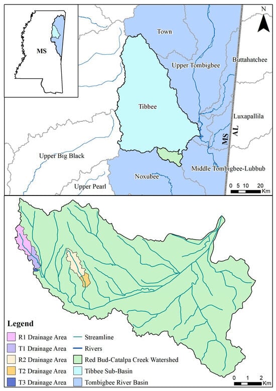
Figure 1.
Map of Red Bud-Catalpa Creek watershed and study site drainage areas, located within the Tibbee Creek Sub-Basin and Tombigbee River Basin (HUC #031601) in northeast Mississippi, USA.
To address these resource concerns, a Water Resources Management Plan was developed and submitted to MDEQ [25,28]. Following approval of the management plan, tributaries of Catalpa Creek that reside within Mississippi State University’s (MSU) H.H. Leveck Animal Research Center (South Farm) and the Bearden Dairy Research Unit (Dairy Farm) were selected for restoration by MDEQ. Critical management areas and conservation practices were selected by local Natural Resource Conservation Service (NRCS) personnel and farm managers. Selected conservation practices were installed according to standards established by the NRCS Field Office Technical Guide [29].
2.2. Study Design
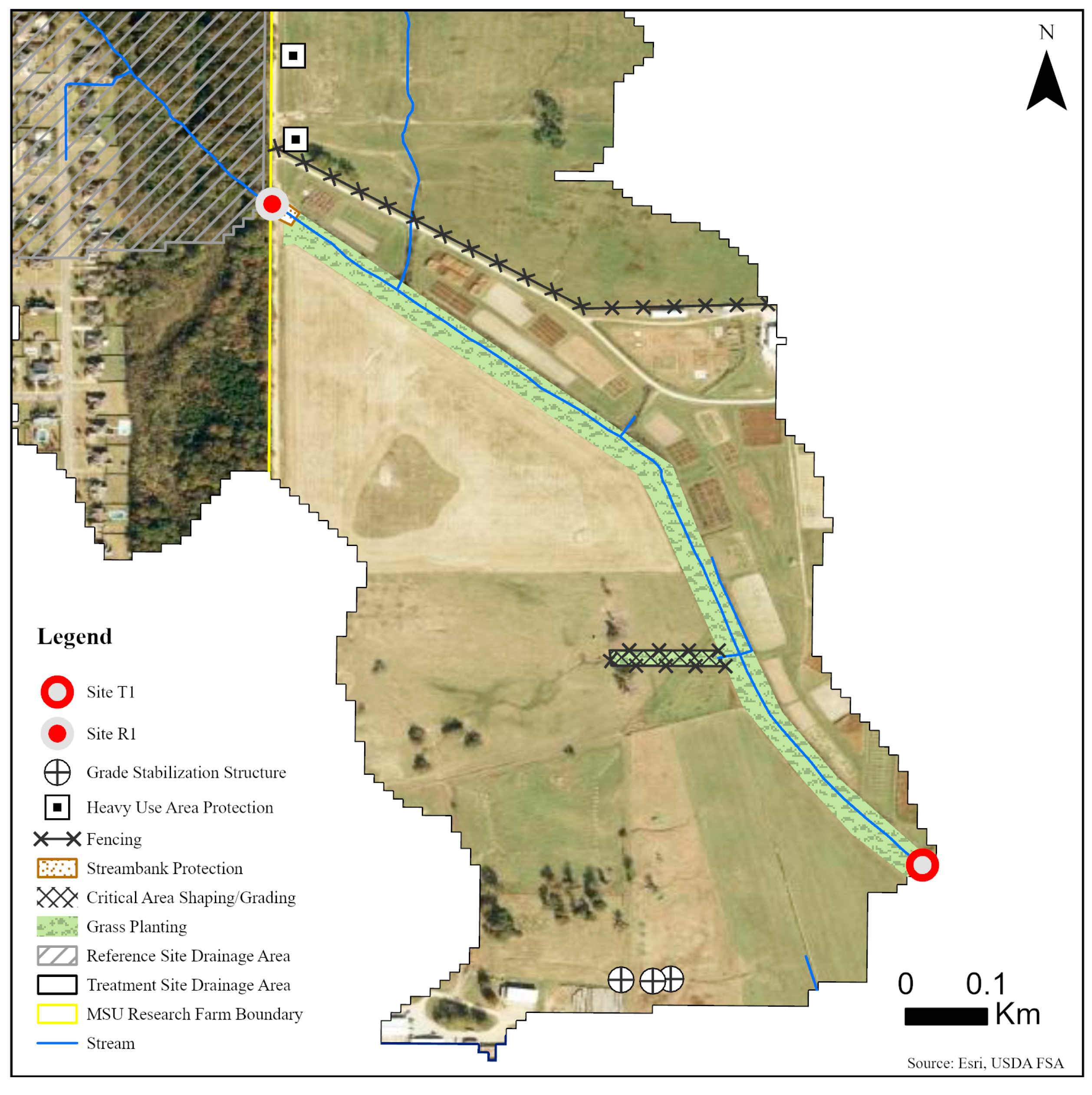
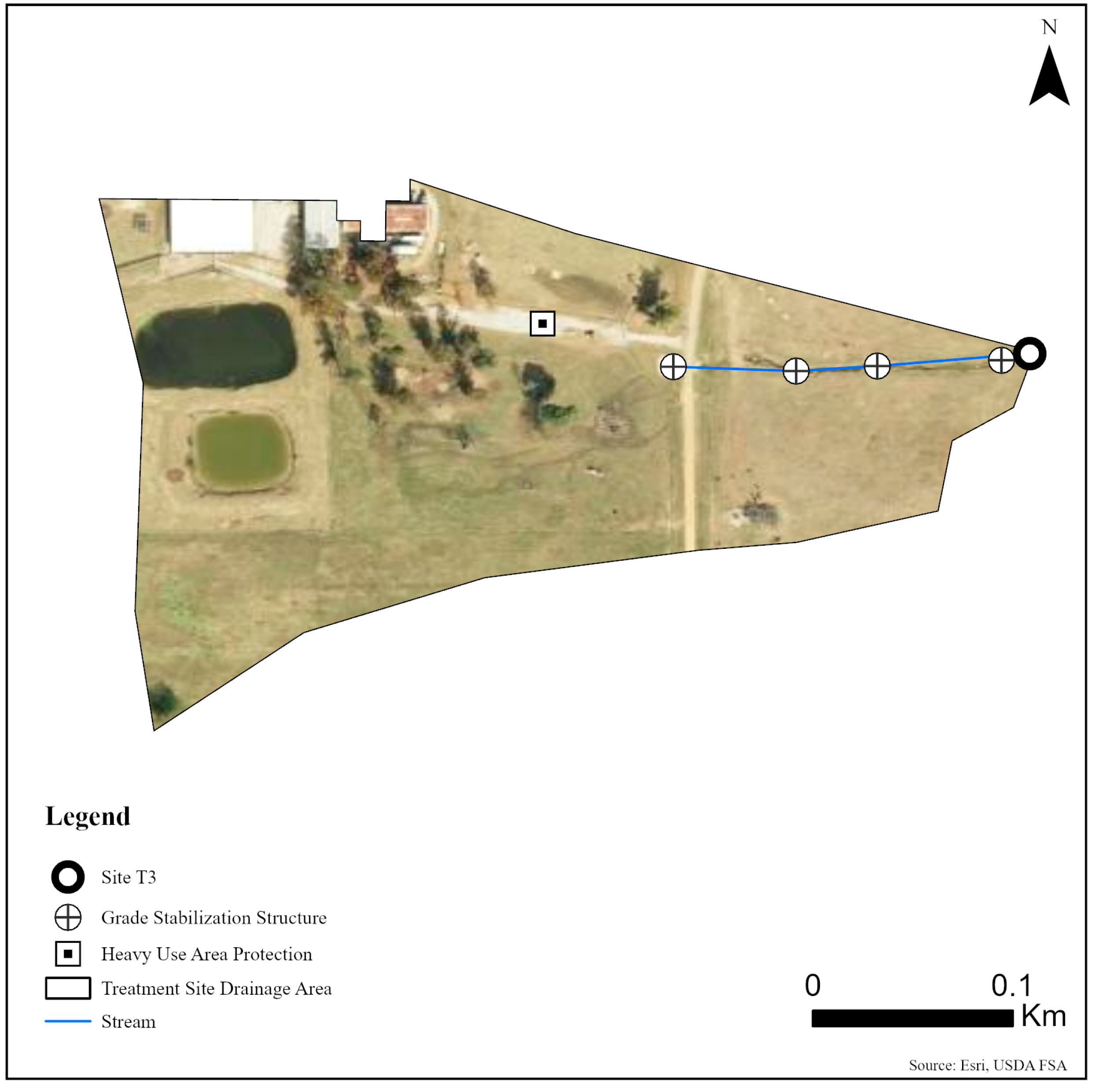
Five sites were monitored along three unnamed tributaries of Catalpa Creek, including two reference sites and three treatment sites. Two of the monitored treatment sites were paired to upstream reference sites: Reference 1 (R1) paired with Treatment 1 (T1) and Reference 2 (R2) paired with Treatment 2 (T2). The site Treatment 3 (T3) was a first-order, edge-of-field outflow, and, therefore, placing a reference site above to assess upstream contributions to water quality was not possible. Drainage areas of each site are shown in Figure 1. Reference sites were upstream of the conservation practice locations. The immediate upstream channels of reference sites had established riparian borders with residential influence further upstream. Treatment sites were downstream of working pasturelands and critical management areas where conservation practices were implemented. The paired site design allowed the pollutant concentrations and loading estimates to be compared between reference sites (baseline data) and treatment sites for each drainage area before and after conservation practice implementation. Drainage area size for sites varied: R1 with 148 ha, T1 with 225 ha, R2 with 145 ha, T2 with 194 ha, and T3 with 5.5 ha. Drainage areas were delineated by the U.S. Geological Survey program StreamStats [30]. Specific practice and site locations are described in Figure 2, Figure 3 and Figure 4.

Figure 2.
Map of monitoring sites and conservation practices planned for sites R1 and T1 on the MSU South Farm in Mississippi State, MS, USA.
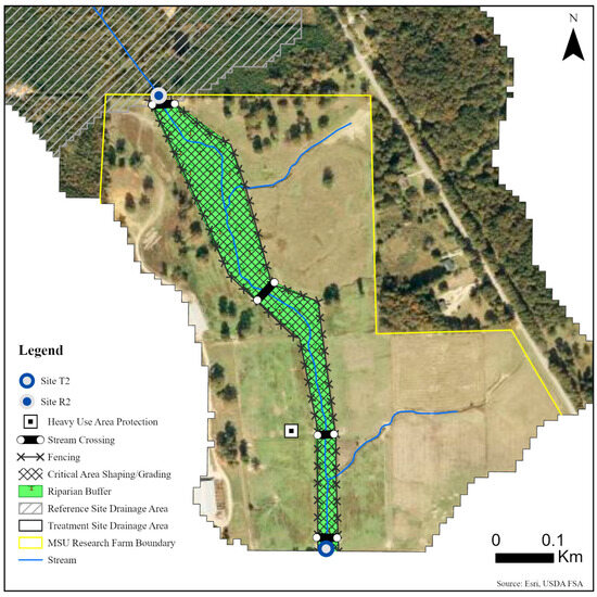
Figure 3.
Map of monitoring sites and conservation practices planned for sites R2 and T2 on the MSU Dairy Farm in Mississippi State, MS, USA.

Figure 4.
Map of monitoring site and conservation practices planned for site T3 on the MSU South Farm in Mississippi State, MS, USA.
Water quality was monitored at all five sites for one year prior to conservation implementation to track baseline water quality conditions and for approximately one year post-conservation practice implementation between January 2018 and December 2019 to determine effects of implementation. The pre–post design allowed for implementation effects to be observed at each treatment site. Samples were collected on a storm-event basis to quantify pollutant concentrations and loads from the surrounding landscapes during rainfall events. Baseflow in these intermittent streams was not consistently measurable; therefore, baseflow was assumed to have a negligible effect on the total load calculations.
2.3. Sampling Procedures
Sampling procedures followed the EPA’s Surface Water Sampling operating procedure [31]. The monitoring equipment used included automated composite samplers (Sigma SD900, American Sigma, Inc., Loveland, CO, USA) deployed at all sites. Samplers were programmed to collect 200 mL grab samples at discharge-based intervals of 600 L to create a 10 L composite sample. Discharge for intervals was measured using ultrasonic Doppler instruments (Starflow 6526J-21, Unidata Pty Ltd., Perth, Australia), which relayed signals to the automated samplers at the specified intervals for sample collection.
During this study, multiple sites experienced several major flooding events and one tornado that compromised sampling equipment. When this occurred, grab samples were collected during the falling hydrographic limb of storm events. In total, 36 composite and 66 grab samples were collected during the pre-treatment period and seven composite and 40 grab samples were collected during the post-treatment period.
Upon collection, all event samples were split into three subsamples of separate sterilized containers for analysis. Two subsamples were placed in duplicate 1 L containers, one of which was preserved immediately with 0.5 mL of 49% sulfuric acid solution. These duplicate subsamples were transported from field sites to the MSU Water Quality Laboratory, refrigerated to maintain a temperature of 4 °C, and shipped within 48 h of sample collection to the MDEQ Office of Pollution Control Laboratory in Pearl, MS, USA, for nutrient and sediment analysis. The third subsample was placed into a 250 mL sterile container and delivered within 24 h of sample collection to the USDA-Agricultural Research Service Genetics and Sustainable Agriculture Research Unit in Mississippi State, MS, USA, for fecal indicator bacterial (FIB) analysis.
2.4. Pollutant Analysis
Nutrient concentrations were measured by MDEQ using a Lachat Flow Injection Analyzer (Lachat Instruments, Loveland, CO, USA). Analysis was conducted using a combination of standard EPA methods for total Kjeldahl nitrogen (Standard Methods 4500-N orgD), ammonia (Standard Methods 4500-NH3G), and nitrate-nitrite (Standard Methods 4500-NO3-) [32]. These nutrients were combined to calculate total nitrogen (TN). Total phosphorus (TP) was measured using Lachat Quik Chem Method 10-115-01-1-C. Total suspended solids (TSS) values were calculated using Clesceri et al. [32] standard methods procedure 2540D. Nutrient and sediment pollutants utilized in the statistical analysis included TN, TP, and TSS.
Fecal indicator bacteria (FIB) pollutants of interest included Escherichia coli (E. coli), enterococci, staphylococci, and Clostridium perfringens (C. perfringens). Water samples (100 mL) were filtered through a 0.45 µm membrane, consistent with standard analysis protocol [33,34,35]. Then, membranes were placed on mTEC agar (E. coli), mEI agar (enterococci), mannitol salt agar (staphylococci), and CP Chromoselect agar (C. perfringens) and incubated [33,34,35]. After respective incubation periods, media were analyzed for enumeration of FIB, and results were recorded as the number of colony-forming units (CFU) per 100 mL [33,34,35,36].
2.5. Statistical Analysis
Exploratory data analysis and summary statistics were used to ensure data quality before further statistical analysis was undertaken. After confirmation of data integrity, pollutant data were tested for normality assumptions using the Shapiro–Wilk test and evaluation of QQ plots [37]. All pollutant variables of interest were determined to have non-normal distributions. Nutrient and sediment variables were not transformed; therefore, the non-parametric Mann–Whitney Signed Rank Test was utilized to test for statistical significance of differences in medians between treatment and reference sites [38]. A post hoc Mann–Whitney U-Test was conducted on significant trends identified in the models to test for differences in medians between pre- and post-implementation periods [38].
FIB counts were log-transformed for descriptive analysis and site-specific data were combined for all treatment sites and all reference sites to increase sample size for statistical analysis. FIB data were categorized by season to prevent the clouding of statistical results, as species counts have been shown to change throughout the year [39]. Samples collected from May to October were classified within the summer season, and samples collected from November to April were classified within the winter season [39]. For FIB data collected during the summer and winter seasons, linear mixed-effects models that compared the analysis of variance between fixed effects of treatment (reference and treatment sites), pre- and post-implementation monitoring periods, and their interaction were used, with precipitation events included as a random variable due to their inherent variability [40]. A Tukey’s post hoc analysis was used to test for significance between pairwise comparisons [40]. For the purposes of this study, significance thresholds of p = 0.05 were set a priori to delineate statistical significance.
3. Results
3.1. General Pollutant Concentrations and Loading
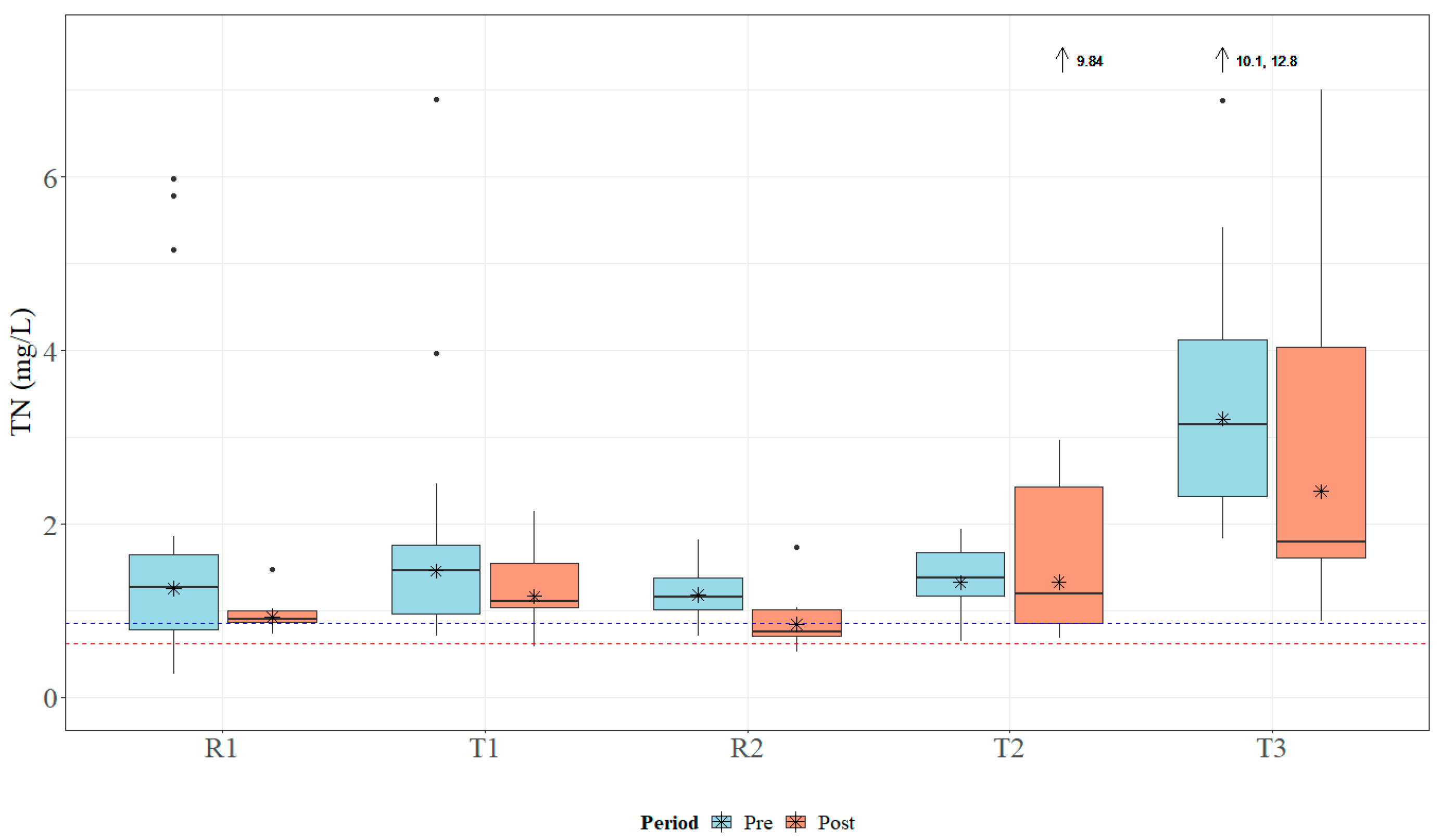
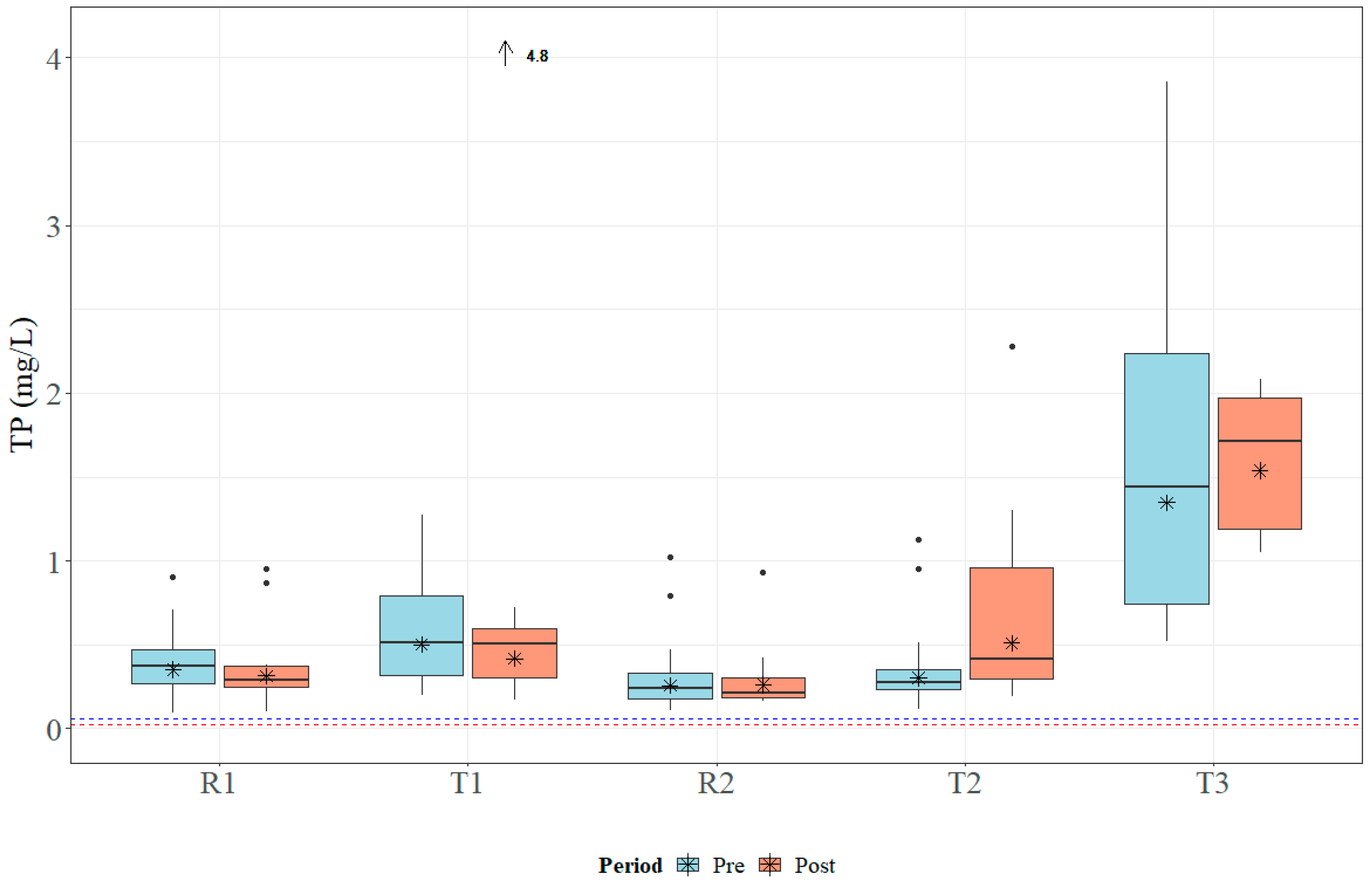
Within the study period, the study sites received approximately 178 cm of rain in 2018 and 203 cm of rain in 2019. Both years registered above the average annual rainfall, which ranges between 127 and 165 cm for the study area [41]. Median TN concentrations ranged from 1.0 to 3.065 mg L−1, which is above MDEQ draft numeric criteria (0.850 mg L−1) and EPA Ecoregion 65a-suggested numeric criteria (0.618 mg L−1) [24,26]. Data for TN concentrations across all sites are presented in Figure 5. Median TP concentrations ranged from 0.23 to 1.54 mg L−1, which is above MDEQ draft numeric criteria (0.060 mg L−1) and EPA Ecoregion 65a-suggested numeric criteria (0.023 mg L−1) [24,26]. Data for TP concentrations across all sites are presented in Figure 6. Median concentrations of TSS ranged from 30.5 to 104.0 mg L−1 (Figure 7); no MDEQ or regional numeric criteria were available to evaluate TSS concentrations. Nutrient and sediment concentrations from samples over the complete study period (2018 and 2019) and the number of collected samples used within the analysis for each site are presented in Table 1.
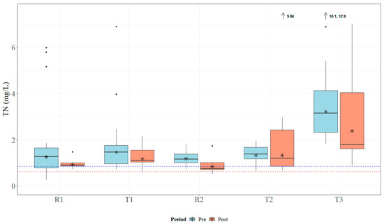
Figure 5.
Boxplots of general total nitrogen (TN) concentrations collected within Catalpa Creek tributaries pre- and post implementation of conservation practices. The blue dashed line (0.850 mg L−1) indicates MDEQ draft numeric criteria for TN concentration for pollutant/stressor response threshold (macroinvertebrate indicators), the red line (0.618 mg L−1) indicates suggested EPA Ecoregion 65a numeric criteria for TN concentrations [24,26]. Lines in boxplots represent medians; asterisks represent means. Dots represent measurements that are statistical outliers. Arrows with numerical values at the top of the figure indicate outliers not included in the figure.
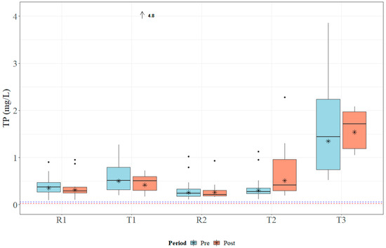
Figure 6.
Boxplots of general total phosphorus (TP) concentrations collected within Catalpa Creek tributaries pre- and post implementation of conservation practices. The blue dashed line (0.060 mg L−1) indicates MDEQ draft numeric criteria for TP concentration for pollutant/stressor response threshold (macroinvertebrate indicators), the red line (0.0225 mg L−1) indicates suggested EPA Ecoregion 65a numeric criteria for TP concentrations [24,26]. Lines in boxplots represent medians; asterisks represent means. Dots represent measurements that are statistical outliers. Arrows with numerical values at the top of the figure indicate outliers not included in the figure.
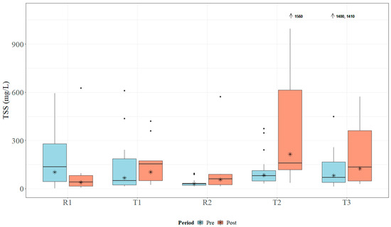
Figure 7.
Boxplots of general total suspended solids (TSS) concentrations collected within Catalpa Creek tributaries pre- and post implementation of conservation practices. Lines in boxplots represent medians; asterisks represent means. Dots represent measurements that are statistical outliers. Arrows with numerical values at the top of the figure indicate outliers not included in the figure.

Table 1.
Descriptions of total nitrogen (TN), total phosphorus (TP), and total suspended solids (TSS) concentrations at Catalpa Creek tributary sites pre- and post implementation of planned practices.
Average TN and TP load estimates for the observed storm events within the study period ranged from 0.08 to 0.76 kg ha−1 and 0.03 to 0.34 kg ha−1, respectively. Average TSS loads ranged from 3.78 to 39.38 kg ha−1 per event. Load estimates of TSS were generally above the MDEQ TMDL sediment requirement for Tibbee Creek Sub-Basin, which is 0.90–4.0 kg ha−1 per day [27]. Estimated nutrient and sediment loads for each site are described in Table 2.
Table 2.
Descriptions of median total nitrogen (TN), total phosphorus (TP), and total suspended solids (TSS) estimated loads at Catalpa Creek tributary sites pre- and post implementation of planned practices. Load (kg ha−1) = event concentration × total event discharge.
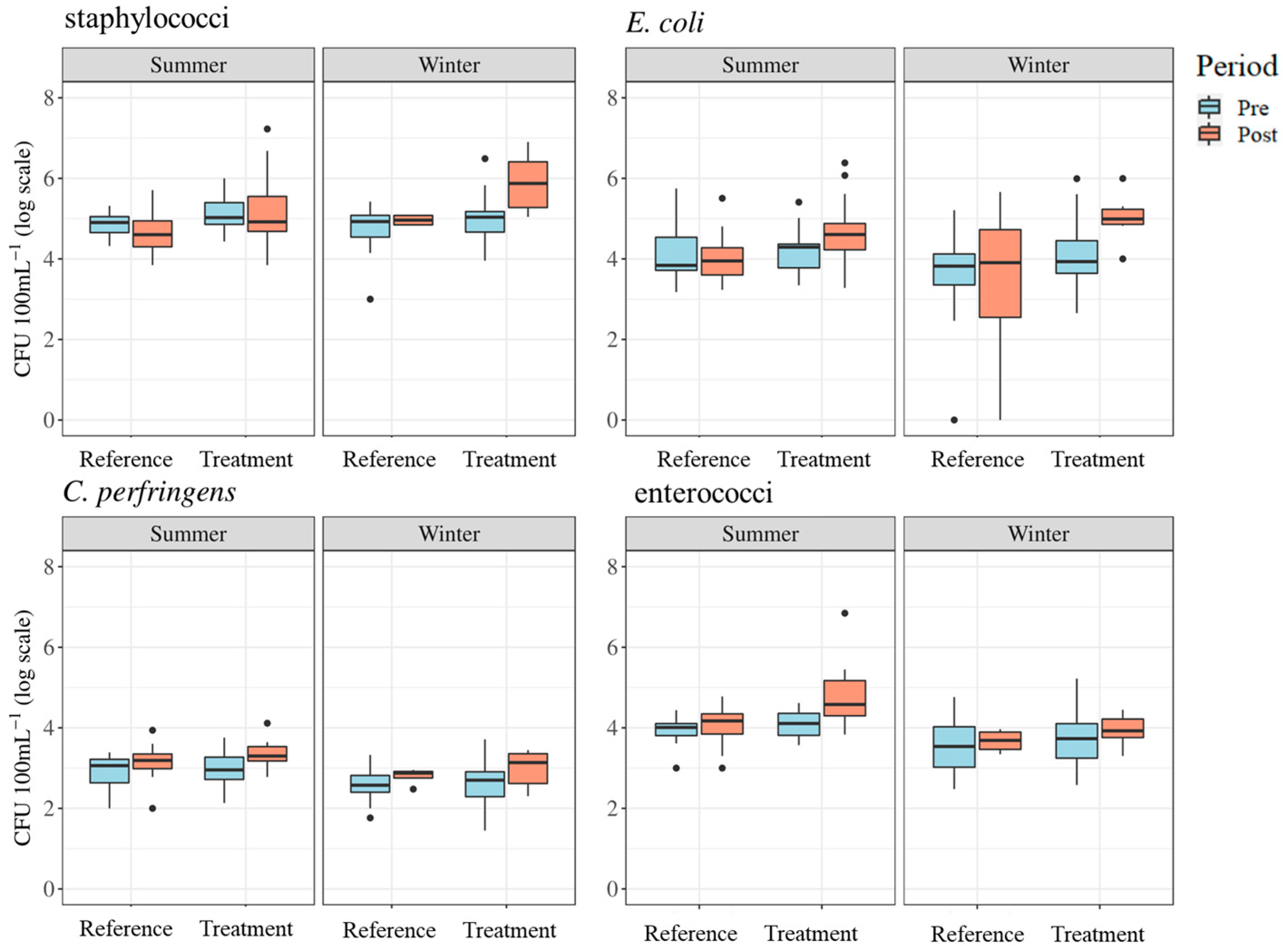
Geometric means of E. coli counts ranged from 10,441 to 42,313 CFU 100 mL−1 in the summer season and 2333 to 104,037 CFU 100 mL−1 in the winter. Geometric means of enterococci ranged from 8670 to 50,446 CFU 100 mL−1 in the summer season and 3661 to 8621 CFU 100 mL−1 during the winter. Staphylococci counts ranged from 43,535 to 144,622 CFU 100 mL−1 in the summer season and from 63,340 to 781,518 CFU 100 mL−1 in the winter. Geometric means for C. perfringens ranged from 678 to 2170 CFU 100 mL−1 in the summer season and 407 to 961 CFU 100 mL−1 in the winter. The distributions of FIB counts by season, site, and period are shown in Figure 8. Data for FIB counts are described by season in Table 3.

Figure 8.
Boxplots of fecal indicator bacteria results for summer and winter seasons representing treatment and reference sites and pre- and post-implementation periods. Dots represent measurements that are statistical outliers.
Table 3.
Summary of FIB levels at Catalpa Creek tributary sites pre- and post implementation of planned practices. Levels are reported as CFU 100 mL−1. All counts are geometric means.
3.2. Reference vs. Treatment Site Concentrations and Loading
Overall, TN and TP concentrations were found to be higher at downstream treatment sites than at upstream reference sites across the entire study period. The R1 site had significantly lower TN concentrations (U = 104, p < 0.01) and TP concentrations (U = 65, p < 0.001) than its paired downstream site T1. The R2 site was found to have significantly lower TN concentrations (U = 104, p < 0.01) and TP concentrations (U = 65, p < 0.001) than its paired downstream site T2. TN concentrations are shown in Figure 5 and TP concentrations are shown in Figure 6. There was no statistical difference in TSS concentrations in samples between paired sites (p > 0.05; Figure 7).
3.3. Pre- vs. Post-Implementation Concentrations and Loading
Sample concentrations for TN, TP, and TSS in both pre- and post-implementation periods are represented in Figure 5, Figure 6, and Figure 7, respectively. Mann–Whitney U tests indicated significant differences in TN concentrations between pre- and post-implementation periods at T3 (U = 126, p < 0.01), with concentrations reduced post implementation. Statistically significant differences were detected in median TSS concentrations at R1 (U = 183.5, p < 0.05), with concentrations reduced post implementation. Mann–Whitney U tests confirmed significant differences in TP (U = 58.5, p < 0.05) and TSS (U = 38.5, p < 0.01) concentrations between periods at T2, with concentrations increasing post implementation. All median runoff concentrations pre- and post implementation are detailed in Table 1.
Pre-implementation TN loads for all sites ranged from 6.86 × 10⁻⁵ to 1.80 kg ha−1, while post-implementation loads ranged from 0.004 to 2.18 kg ha−1. Loads of TP varied for all sites between 3.43 × 10⁻⁵ and 0.639 kg ha−1 pre-implementation and between 3.00 × 10⁻⁴ and 2.43 kg ha−1 post implementation. Finally, TSS loads for all sites during the pre-implementation period were between 0.021 and 59.5 kg ha−1, while post-implementation loads ranged from 0.205 to 507.6 kg ha−1. Estimated pre- and post-implementation loads are described in Table 2.
3.4. Fecal Indicator Bacteria Levels
Differences in FIB levels between pre- and post-implementation periods varied (Figure 8). Linear mixed-effects model results indicated statistically significant differences between reference and treatment sites (p < 0.05) and between treatment periods (p < 0.05) for staphylococci in the winter season. The results also indicated statistically significant differences between reference and treatment sites (p < 0.05) and treatment periods (p < 0.05) in E. coli levels during the winter season (see Table 4). Tukey’s post hoc pairwise comparisons confirmed significant differences between post-implementation reference and post-implementation treatment sites (p < 0.01), and pre- and post-implementation treatment periods at treatment sites (p < 0.01) for staphylococci and E. coli levels in the winter season. This means that, practically, for both staphylococci and E. coli in the winter, these FIB levels were greater post implementation at treatment sites compared to post implementation at reference sites and compared to pre-implementation at the treatment sites. No significant differences were found in any summer periods for staphylococci, summer periods for E. coli, or either winter or summer periods for C. perfringens and enterococci.
Table 4.
Linear mixed model results (p-values) of pathogen analysis for summer and winter seasons between periods, sites, and treatment.
4. Discussion
All five sites within this study, including the control reference sites, were found to have measures of central tendency of storm-event pollutant concentrations above MDEQ draft numeric criteria and EPA-recommended guidelines for TN and TP. Additionally, some sites had TSS loads above the MDEQ TMDL and E. coli and enterococci counts above recommended levels [24,26]. Pollutant concentrations exceeding water quality criteria ultimately indicate that tributaries within this study remained impaired one year after implementation of the conservation practices. Pollutant concentrations and loading measurements warrant consideration for continued monitoring, with special attention to pathogen levels in surface water. Sediment and nutrients were thought to be the primary threat in this watershed and are the primary focus of most surface water monitoring programs. However, this study demonstrates that FIB can and should supplement traditional monitoring efforts in order to gain a more holistic view of watershed function.
Elevated pollutant levels and loss of sediment via gully expansion in pastures are exacerbated by cattle presence and use patterns [7,42]. Exclusion fencing for livestock is a widely accepted method for the effective, immediate reduction in cattle nutrient input, FIB deposition, and soil degradation from loafing within small riparian areas, which was the goal of the fencing planned in this study [6,43,44]. All treatment sites in this study drained active cattle pastures, with two of the three treatment sites having a highly active livestock presence near or within the monitored drainage channel. However, exclusion fencing was not fully installed in the T2 drainage area until after the completion of this study. As a result, the riparian buffer installed to reduce runoff pollution had been browsed by cattle and had not reached maturation. Therefore, continued livestock access to the streambank until completion of the fencing installation between the R2 and T2 sites was a major contributing factor to the elevated pollutant concentrations (TN, TP, and FIBs) at the downstream T2 monitoring site throughout this study. In consideration of the elevated FIB results, a similar study by Wagner et al. [45] found that E. coli counts did not change in the short-term in small agricultural watersheds, even when grazing management was improved with conservation practices. This lack of improvement in FIB at T2 and the other treatment sites could be attributed to a number of causes, including fecal bacteria from wildlife, the transport of sediment-bound bacteria, and the retention of bacteria in environments with high soil moisture [35,46,47,48]. It is likely that all of these factors were present during this study as in the study by Wagner et al. [45], resulting in minimal differences in FIB counts after treatment.
The highest values for pollutants generally occurred at treatment site T3, which contained a first-order stream within a small, pasture-dominated watershed, downhill of a high-traffic beef cattle pasture area. However, T3 was also the only site to have a detectable reduction in TN due to conservation practice implementation. Previous studies by Lowrance et al. [49] and Buck et al. [42] hypothesized that the local land use around first-order streams, particularly the abundance and movement of livestock, is highly correlated with the first-order stream water quality because of the immediate spatial interaction of runoff with pollutants. Site T3, as a first-order stream, had a more direct interaction with land in its total drainage area and therefore higher concentrations of pollutants. Its size and interaction intensity with the drainage area are also hypothesized as the reason it was the only site to see positive short-term results from conservation practice implementation [42,49].
With only a partial conservation implementation at other sites, T3 was also the only site to receive the full complement of planned conservation practices. Additionally, grass buffers were allowed to be established along and within the drainage channel. A high practice implementation density and placement along low-order streams have been proposed by several studies to be the most effective strategy for achieving meaningful reductions in water quality parameters of concern [11,15,16]. The riparian cover of first-order streams has also been hypothesized to be highly influential towards the concentrations of downstream water quality parameters, specifically for TN and TP concentrations [11,19,20]. Furthermore, the type, age, and width of the riparian cover were found to influence the uptake of nitrogen within buffers—with woody, younger, or wider footprints having greater percentages of nitrogen uptake than herbaceous, older, or narrower buffers [50,51]. These studies support the observation that the presence of a new and adequately wide herbaceous buffer at T3 likely helped with nitrogen uptake in the post-implementation period, reducing the observed TN.
In contrast to conservation implementation and monitoring along first-order streams, determining the conservation practice effectiveness near larger streams with highly incised streambanks poses much greater challenges. The channel morphology of an incised stream exacerbates pollutant loading because of the positive feedback loop between increased stormflow capacity, sediment loading, and streambank failure [17,52]. The incoming discharge from upstream sources and processes within these altered streams has more influence on the in-stream water quality than the immediate surrounding landscape does, which makes addressing degradation in these channels difficult, especially if the land upstream is stewarded by a different landowner [18]. This hydrological barrier was likely a major factor in the water quality concentrations and loading measured throughout this study at the R1 and T1 sites, which were located on a heavily incised portion of the tributary of interest. To fully address conservation needs in systems with heavily modified agricultural streams, the intensive alteration of channel morphology back to natural equilibriums—such as gradual sloping banks to reduce erosion potential, meandering channel path courses that slow water velocity, and the establishment of riparian buffers to stabilize soil—would be needed [18]. However, this type of comprehensive channel restoration is difficult to fully implement and is not accessible to all landowners. Such an extreme modification was not feasible within the duration of this study.
The development of water quality criteria and the study of conservation effectiveness are crucial to the ongoing efforts to address broad-scale pollutant impacts, such as those in the Gulf of Mexico Hypoxia Zone. Though it may be tempting to neatly determine and address sources of water quality issues within larger watershed contexts, the true effectiveness of practices and conservation efforts is realized when planned at much smaller, local scales [19,21,42,49]. These smaller catchment areas, especially those of first-order streams, interact directly with landscape sources of pollutants. The sheer number of first-order streams, foundational in the dendritic distribution of streams and rivers, makes them integral in the pollutant transport process and exacerbates pollutant effects downstream [19]. Thus, reductions in TN concentrations at sites such as T3 are promising in the context of potential widespread conservation implementation efforts directed at first-order stream sites.
The complexity of conservation practice adoption and evaluation creates several challenges for researchers, landowners, and agricultural producers interested in efficiently and effectively implementing conservation practices. Private individuals may not have the resources (time, spatial, financial) to participate in conservation efforts at the required density and over the necessary time frame needed to overcome ecological thresholds. Additionally, confounding environmental variables, such as high rainfall events and droughts, may thwart efforts to implement and functionally establish even the best intentioned conservation practices. This study serves as an example of the detrimental effects of conservation practice implementation that can be observed in the short-term, especially if the practice density is not met, is significantly delayed due to common logistical hurdles, or is interrupted by historical weather events.
The authors have several recommendations for future research and adjustments in the field of environmental policy and conservation application as a result of this study. First, further research into quantifying practice density thresholds and the prioritization of practice selection and placement (such as precision conservation applications) would help determine the most effective and efficient implementation plans for farm-level conservation. The conversion of these types of studies into predictive Geographic Information System programs used for conservation planning, similar to processes in precision agriculture research occurring in cropping systems, would further enhance the applicability and usefulness. Second, FIB levels should be included in water quality studies as a standard parameter, as they are an important factor in overall stream health and impairment determinations. Even when sources for nutrients and sediment loads have been mitigated through conservation practice implementation, FIB levels can remain high, indicating lingering impairment issues. Additionally, streams can still be impaired by FIB through sources other than agriculture after conservation practices have been implemented, indicating that further work within the watershed may be needed (such as with malfunctioning septic systems). Third, a network of collaboration at the watershed level between government agencies, communities, and individual landowners and producers is also encouraged to create a larger impact with the adoption of field- and farm-level conservation plans. Such collaborations exist and are extremely strong in some localities but are lacking in others. These relationships should be strengthened whenever possible. Finally, funding and environmental policy should be adjusted to reflect the natural lag time that occurs in water quality monitoring, as there is currently a discrepancy between the length of funding for projects and the water quality response necessary to determine the conservation practice effectiveness and remove streams from impairment lists. A strong framework exists for meaningful continued research, conservation practice implementation, and the improvement in water resources through federal, state, and private collaboration. These conservation principles and performance measures simply need to be more accurately aligned with the intrinsic behavior of ecosystems and producers to increase positive field-level impacts.
5. Conclusions
The results of this study showed minimal, and in some contexts detrimental, impacts of conservation practice implementation on water quality one year after the conservation practice implementation began. In this short timeframe, conservation efforts were only effective in reducing nitrogen when applied at a small, pasture-level scope. This scope required the least amount of time and resources for construction completion and was the most efficient at reducing (or at least maintaining) pollutant concentrations in the short-term. This study should serve as guidance for landowners and agricultural producers to prioritize concentrated (and fully completed) suites of practices in small, critical areas that can make a practical difference with lower input costs, rather than decentralized practices that are inefficiently scattered across the landscape. Additionally, FIB were more prevalent in this study than expected, especially in sites downstream of livestock pastures after conservation practice implementation. The FIB were a reliable indicator of the continued impacts of livestock production on the streams, even after conservation practice implementation. The presence of FIB should be strongly considered when designing water quality policy, monitoring studies, and field-level applications. Other short-term studies in different landscapes would help clarify if the results of this short-term study are replicable in other conservation practice sites. Additionally, long-term monitoring of the site used in this specific study would be beneficial for understanding the effects of conservation practice maturation on the nutrient, sediment, and FIB presence in the watershed, especially in comparison to the short-term monitoring results.
Author Contributions
Conceptualization, L.M.B., J.J.R.-A., T.S., J.M.P.C., L.W.B.J. and B.H.B.; methodology, J.P.B., R.K.S. and B.H.B.; formal analysis, A.M. and A.L.; investigation, A.M., J.P.B., R.K.S., J.J.R.-A., T.S., J.M.P.C., L.W.B.J. and B.H.B.; data curation, A.M., J.P.B., R.K.S. and A.L.; writing—original draft preparation, A.M., J.P.B., R.K.S., L.M.B. and B.H.B.; writing—review and editing, A.L., J.J.R.-A., T.S., J.M.P.C. and L.W.B.J.; visualization, A.M.; supervision, L.M.B. and B.H.B.; project administration, B.H.B.; funding acquisition, L.M.B., J.J.R.-A., T.S., J.M.P.C., L.W.B.J. and B.H.B. All authors have read and agreed to the published version of the manuscript.
Funding
This work was supported by the Mississippi Department of Environmental Quality 319 funding grant no. 18-00049.
Data Availability Statement
The data presented in this study are available from the corresponding author upon reasonable request.
Acknowledgments
This publication is a contribution of the Mississippi Agricultural and Forestry Experiment Station. The authors would like to thank the H.H. Leveck Animal Facility operations management team, local Natural Resources Conservation Service personnel, and research assistants who helped with sample collection.
Conflicts of Interest
The authors declare no conflicts of interest.
References
- U.S. Environmental Protection Agency. A National Evaluation of the Clean Water Act Section 319 Program; Office of Wetlands, Ocean, & Watersheds: Washington, DC, USA, 2011. [Google Scholar]
- U.S. Environmental Protection Agency. [Pie Graph of Assessed Rivers and Streams]. National Summary Water Quality Attainment in Assessed Rivers and Streams. Available online: https://ofmpub.epa.gov/waters10/attains_nation_cy.control (accessed on 1 January 2020).
- Evans, A.E.; Mateo-Sagasta, J.; Qadir, M.; Boelee, E.; Ippolito, A. Agricultural water pollution: Key knowledge gaps and research needs. Curr. Opin. Environ. Sustain. 2019, 36, 20–27. [Google Scholar] [CrossRef]
- Hooda, P.S.; Edwards, A.C.; Anderson, H.A.; Miller, A. A review of water quality concerns in livestock farming areas. Sci. Total Environ. 2000, 250, 143–167. [Google Scholar] [CrossRef]
- Jordan, M.A.; Casteneda, A.J.; Smiley, P.C.; Gillespie, R.B.; Smith, D.R.; King, D.R. Influence of instream habitat and water chemistry on amphibians in channelized agricultural headwater streams. Agric. Ecosyst. Environ. 2016, 230, 87–97. [Google Scholar] [CrossRef]
- Clary, C.R.; Redmon, L.; Gentry, T.; Wagner, K.; Lyons, R. Nonriparian shade as a water quality best management practice for grazing-lands: A case study. Rangelands 2016, 38, 129–137. [Google Scholar] [CrossRef]
- Zaimes, G.N.; Schultz, R.C.; Tufekcioglu, M. Gully and stream bank erosion in three pastures with different management in southeast Iowa. J. Iowa Acad. Sci. 2009, 116, 1–8. [Google Scholar]
- Baker, B.H.; Kroger, R.; Prevost, J.D.; Pierce, T.; Ramirez-Avila, J.J.; Prince Czarnecki, J.M.; Faust, D.; Flora, C. A field-scale investigation of nutrient and sediment reduction efficiencies of a low-technology best management practice: Low-grade weirs. Ecol. Eng. 2016, 91, 240–248. [Google Scholar] [CrossRef]
- Kroger, R.; Holland, M.M.; Moore, M.T.; Cooper, C.M. Agricultural drainage ditches mitigate phosphorus loads as a function of hydrological variability. J. Environ. Qual. 2008, 37, 107–113. [Google Scholar] [CrossRef]
- Ward, A.; Sharpley, A.; Miller, K.; Dick, W.; Hoorman, J.; Fulton, J.; LaBarge, G.A. An assessment of in-field nutrient best management practices for agricultural crop systems with subsurface drainage. J. Soil Water Conserv. 2018, 73, 5A–10A. [Google Scholar] [CrossRef]
- Osborne, L.L.; Kovacic, D.A. Riparian vegetated buffer strips in water-quality restoration and stream management. Freshw. Biol. 1993, 29, 243–258. [Google Scholar] [CrossRef]
- Musser, S.R.; Grafe, J.; Ortega-Achury, S.L.; Ramirez-Avila, J. Influence of riparian vegetation on stream health and water quality. In Proceedings of the World Environmental and Water Resources Congress 2019, Pittsburgh, PA, USA, 19–23 May 2019; pp. 59–67. [Google Scholar] [CrossRef]
- Noble-Cagle, T.; Musser, S.; Richardson, B.; Ramirez-Avila, J.J. Stream macroinvertebrate diversity and water quality of Catalpa Creek in Mississippi. In Proceedings of the World Environmental and Water Resources Congress 2019, Pittsburgh, PA, USA, 19–23 May 2019; pp. 68–77. [Google Scholar] [CrossRef]
- Yates, A.G.; Bailey, R.C.; Schwindt, J.A. Effectiveness of best management practices in improving stream ecosystem quality. Hydrobiologia 2007, 583, 331–334. [Google Scholar] [CrossRef]
- Baker, B.H.; Prince Czarnecki, J.M.; Omer, A.R.; Aldridge, C.A.; Kroger, R.; Prevost, J.D. Nutrient and sediment runoff from agricultural landscapes with varying suites of conservation practices in the Mississippi Alluvial Valley. J. Soil Water Conserv. 2018, 73, 75–85. [Google Scholar] [CrossRef]
- Kroger, R.; Prince Czarnecki, J.M.; Tank, J.L.; Christopher, S.F.; Witter, J.D. Implementing innovative drainage management practices in the Mississippi River Basin to enhance nutrient reductions. J. Am. Water Resour. Assoc. 2015, 51, 1020–1028. [Google Scholar] [CrossRef]
- Dabney, S.M.; Shields, F.D.; Bingner, R.L.; Kuhnle, R.A.; Rigby, J.R. Watershed management for erosion and sedimentation control case study: Goodwin Creek, Panola County, MS. In Soil Water and Agronomic Productivity; Lal, R., Stewart, B.A., Eds.; CRC Press: Boca Raton, FL, USA, 2012; pp. 539–556. ISBN 9781439850794. [Google Scholar]
- Shields, F.D.; Knight, S.S.; Cooper, C.M. Can warmwater streams be rehabilitated using watershed-scale standard erosion control measures alone? Environ. Manag. 2007, 40, 62–79. [Google Scholar] [CrossRef] [PubMed]
- Alexander, R.B.; Boyer, E.W.; Smith, R.A.; Schwarz, G.E.; Moore, R.B. The role of headwater streams in downstream water quality. J. Am. Water Resour. Assoc. 2007, 43, 41–59. [Google Scholar] [CrossRef] [PubMed]
- Dodds, W.K.; Oakes, R.M. Headwater influences on downstream water quality. Environ. Manag. 2008, 41, 367–377. [Google Scholar] [CrossRef]
- Meals, D.W.; Dressing, S.A.; Davenport, T.E. Lag time in water quality response to best management practices: A review. J. Environ. Qual. 2010, 39, 85–96. [Google Scholar] [CrossRef]
- Prokopy, L.S.; Genskow, K.; Asher, J.; Baumgart-Getz, A.; Bonnell, J.E.; Allread, S.B.; Curtis, C.; Floress, K.; McDermaid, K.; Power, R.; et al. Designing a regional system of social indicators to evaluate nonpoint source projects. J. Ext. 2009, 47, 1. [Google Scholar]
- Harmel, R.D.; King, K.W.; Haggard, B.E.; Wren, D.G.; Sheridan, J.M. Practical guidance for discharge and water quality data collection on small watersheds. Trans. ASABE 2006, 49, 937–948. [Google Scholar] [CrossRef]
- U.S. Environmental Protection Agency. Ambient Water Quality Criteria Recommendations: Information Supporting the Development of State and Tribal Nutrient Criteria for Rivers and Streams in Nutrient Ecoregion IX (EPA-822-B-00-019); Office of Water: Washington, DC, USA, 2000. Available online: https://www.epa.gov/sites/default/files/documents/rivers9.pdf (accessed on 1 January 2020).
- Ramirez-Avila, J.; Schauwecker, T.J.; Czarnecki Prince, J.M. Catalpa Creek Watershed Planning, Restoration, and Protection Project. In Proceedings of the XIX Conferenza Nazionale della Società Italiana degli Urbanisti (SIU), Catania, Italy, 16–18 June 2016. [Google Scholar]
- Mississippi Department of Environmental Quality. Mississippi 2016 Section 303(d) List of Impaired Water Bodies; Mississippi Department of Environmental Quality: Jackson, MS, USA, 2016. Available online: https://www.mdeq.ms.gov/wp-content/uploads/2017/06/2016_Adopted_Section_303d_List.pdf (accessed on 1 January 2020).
- Mississippi Department of Environmental Quality. Total Maximum Daily Load Tombigbee River Basin Designated Streams in HUC 03160104 (Tibbee Creek) for Impairment Due to Sediment; Mississippi Department of Environmental Quality: Jackson, MS, USA, 2007. Available online: https://www.mdeq.ms.gov/wp-content/uploads/2006/12/TombigbeeRB03160104SedimentJan07.pdf (accessed on 1 January 2020).
- Mississippi State University. Water Resources Management Plan for the Red Bud-Catalpa Creek Watershed. Available online: https://www.cee.msstate.edu/wp-content/uploads/WRMP.pdf (accessed on 1 January 2020).
- Natural Resources Conservation Service, U.S. Department of Agriculture. NRCS Field Office Technical Guide; Natural Resources Conservation Service: Washington, DC, USA, 2020.
- U.S. Geological Survey. The StreamStats Program for Mississippi. Available online: http://water.usgs.gov/osw/streamstats/mississippi.html (accessed on 1 January 2020).
- Decker, C.; Simmons, K. Surface Water Sampling [SESDPROC-201-R3]; Region 4 USEPA Science and Ecosystem Support Division: Athens, GA, USA, 2013. [Google Scholar]
- Clesceri, L.S.; Greenberg, A.E.; Eaton, A.D. Standard Methods for the Examination of Water and Wastewater, 20th ed.; American Public Health Association: Washington, DC, USA, 2013. [Google Scholar]
- Santiago-Rodriguez, T.; Kinzelman, J.; Toranzos, G. Current and developing methods for the detection of microbial indicators in environmental freshwaters and drinking waters. In Manual of Environmental Microbiology, 4th ed.; Yates, M., Nakatsu, C., Miller, R., Pillai, S., Eds.; ASM Press: Washington, DC, USA, 2015; ISBN 978-1-683-67074-2. [Google Scholar]
- U.S. Environmental Protection Agency. Method 1103.1: Escherichia coli (E. coli) in Water by Membrane Filtration Using Membrane-Thermotolerant Escherichia coli Agar (mTEC) (EPA-821-R-10-002); Office of Water: Washington, DC, USA, 2010.
- Brooks, J.P.; Smith, R.K.; Aldridge, C.A.; Chaney, B.; Omer, A.; Dentinger, J.; Street, G.M.; Baker, B.H. A preliminary investigation of wild pig (Sus scrofa) impacts in water quality. J. Environ. Qual. 2020, 49, 27–37. [Google Scholar] [CrossRef]
- Rhodehamel, E.J.; Harmon, S.M. Clostridium perfringens. In Bacteriological Analytical Manual, 8th ed.; FDA: Silver Spring, MD, USA, 2001. [Google Scholar]
- Hirsch, R.M.; Slack, J.R. A nonparametric trend test for seasonal data with serial dependence. Water Resour. Res. 1984, 20, 727–732. [Google Scholar] [CrossRef]
- Shapiro, S.S.; Wilk, M.B.; Chen, H.J. A comparative study of various tests for normality. J. Am. Stat. Assoc. 1968, 63, 1343–1372. [Google Scholar] [CrossRef]
- Hathaway, J.M.; Krometis, L.H.; Hunt, W.F. Exploring seasonality in Escherichia coli and fecal coliform ratios in urban watersheds. J. Irrig. Drain. Eng. 2014, 140, 04014003. [Google Scholar] [CrossRef]
- Bates, D.; Maechler, M.; Bolker, B.; Walker, S. Fitting linear mixed-effects models using lme4. J. Stat. Softw. 2015, 67, 1–48. [Google Scholar] [CrossRef]
- National Oceanic and Atmospheric Administration. Map of Annual Precipitation Totals (Advanced Hydrologic Precipitation Service Precipitation Analysis). Available online: https://water.weather.gov/precip/ (accessed on 1 January 2020).
- Buck, O.; Niyogi, D.K.; Townsend, C.R. Scale-dependence of land use effects on water quality of streams in agricultural catchments. Environ. Pollut. 2004, 130, 287–299. [Google Scholar] [CrossRef] [PubMed]
- Peterson, B.J.; Wollheim, W.M.; Mulholland, P.J.; Webster, J.R.; Meyer, J.L.; Tank, J.L.; Marti, E.; Bowden, W.B.; Valett, H.M.; Hershey, A.E.; et al. Control of nitrogen export from watersheds by headwater streams. Science 2001, 292, 86–90. [Google Scholar] [CrossRef] [PubMed]
- Weidhaas, J.; Anderson, A.; Jamal, R. Elucidating waterborne pathogen presence and aiding source apportionment in an impaired system. Appl. Environ. Microbiol. 2018, 84, 1–13. [Google Scholar] [CrossRef] [PubMed]
- Wagner, K.L.; Gregory, L.; Gerlich, J.A.; Rhodes, E.C.; deVilleneuve, S. Edge-of-field runoff analysis following grazing and silvicultural best management practices in northeast Texas. Water 2023, 15, 3537. [Google Scholar] [CrossRef]
- Ferguson, C.M.; Coote, B.G.; Ashbolt, N.J.; Stevenson, I.M. Relationships between indicators, pathogens, and water quality in an estuarine system. Water Resour. 1996, 30, 2045–2054. [Google Scholar] [CrossRef]
- Fraser, R.H.; Barten, P.K.; Pinney, D.A. Predicting stream pathogen loading from livestock using a geographical information system-based delivery model. J. Environ. Qual. 1998, 27, 935–945. [Google Scholar] [CrossRef]
- Sinton, L.W.; Braithwaite, R.R.; Hall, C.H.; Mackenzie, M.L. Survival of indicator and pathogenic bacteria in bovine feces on pasture. Appl. Environ. Microbiol. 2007, 73, 7917–7925. [Google Scholar] [CrossRef]
- Lowrance, R.; Altier, L.S.; Newbold, J.D.; Schnabel, R.R.; Groffman, P.M.; Denver, J.M.; Correll, D.L.; Gilliam, J.W.; Robinson, J.L.; Brinsfield, R.B.; et al. Water quality functions of riparian forest buffers in Chesapeake Bay watersheds. Environ. Manag. 1997, 21, 687–712. [Google Scholar] [CrossRef] [PubMed]
- Mayer, P.M.; Reynolds, S.K.; McCutchen, M.D.; Canfield, T.J. Meta-analysis of nitrogen removal in riparian buffers. J. Environ. Qual. 2007, 36, 1172–1180. [Google Scholar] [CrossRef] [PubMed]
- Valkama, E.; Usva, K.; Saarinen, M.; Uusi-Kamppa, J. A meta-analysis of nutrient retention by buffer zones. J. Environ. Qual. 2018, 48, 270–279. [Google Scholar] [CrossRef] [PubMed]
- Simon, A. A model of channel response in disturbed alluvial channels. Earth Surf. Process. Landf. 1989, 14, 11–26. [Google Scholar] [CrossRef]


Disclaimer/Publisher’s Note: The statements, opinions and data contained in all publications are solely those of the individual author(s) and contributor(s) and not of MDPI and/or the editor(s). MDPI and/or the editor(s) disclaim responsibility for any injury to people or property resulting from any ideas, methods, instructions or products referred to in the content. |
© 2024 by the authors. Licensee MDPI, Basel, Switzerland. This article is an open access article distributed under the terms and conditions of the Creative Commons Attribution (CC BY) license (https://creativecommons.org/licenses/by/4.0/).