

Vulnerability Assessment of Groundwater Influenced Ecosystems in the Northeastern United States


Abstract
1. Introduction
2. Methods
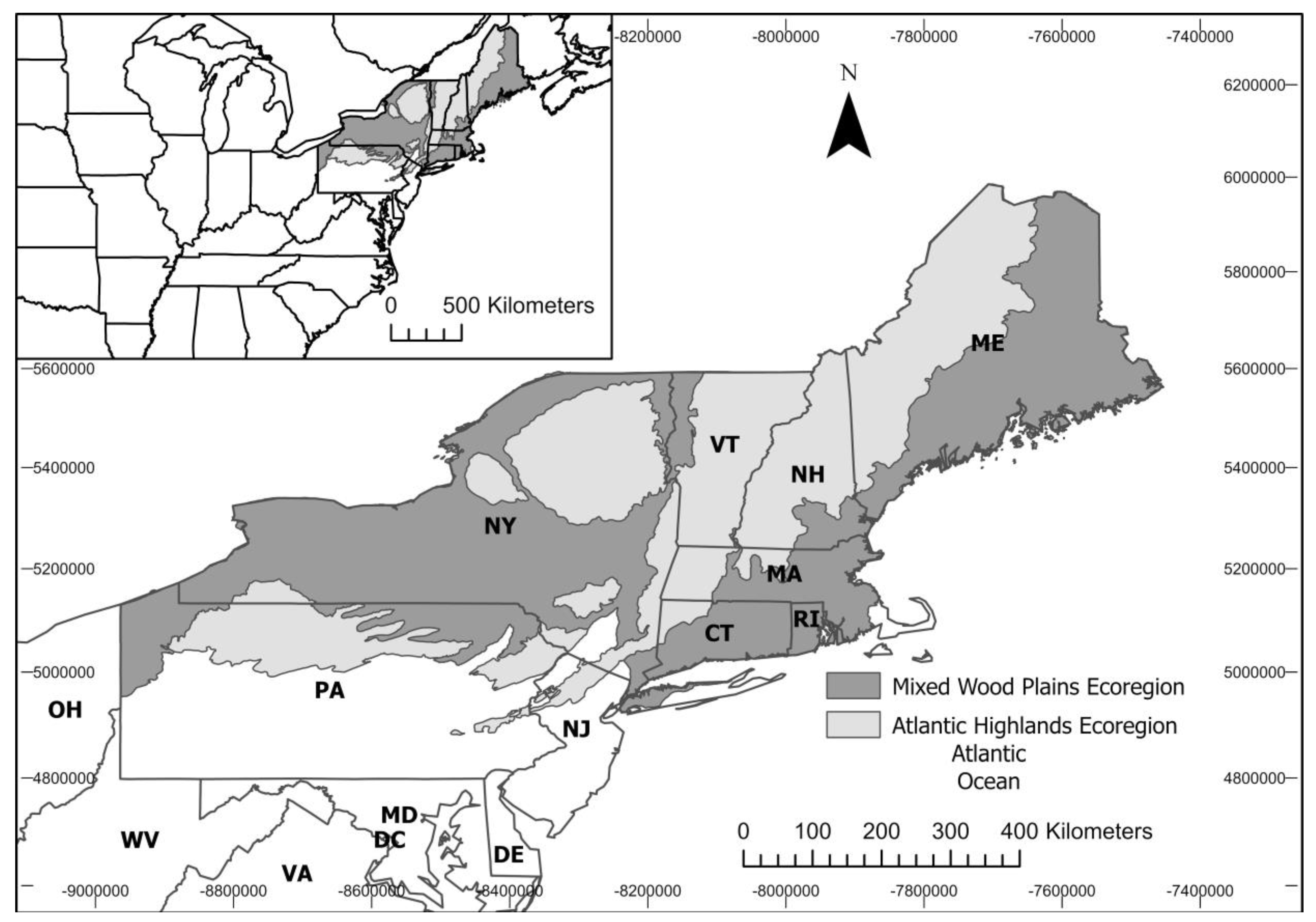
2.1. Study Area
2.2. Vulnerability Framework
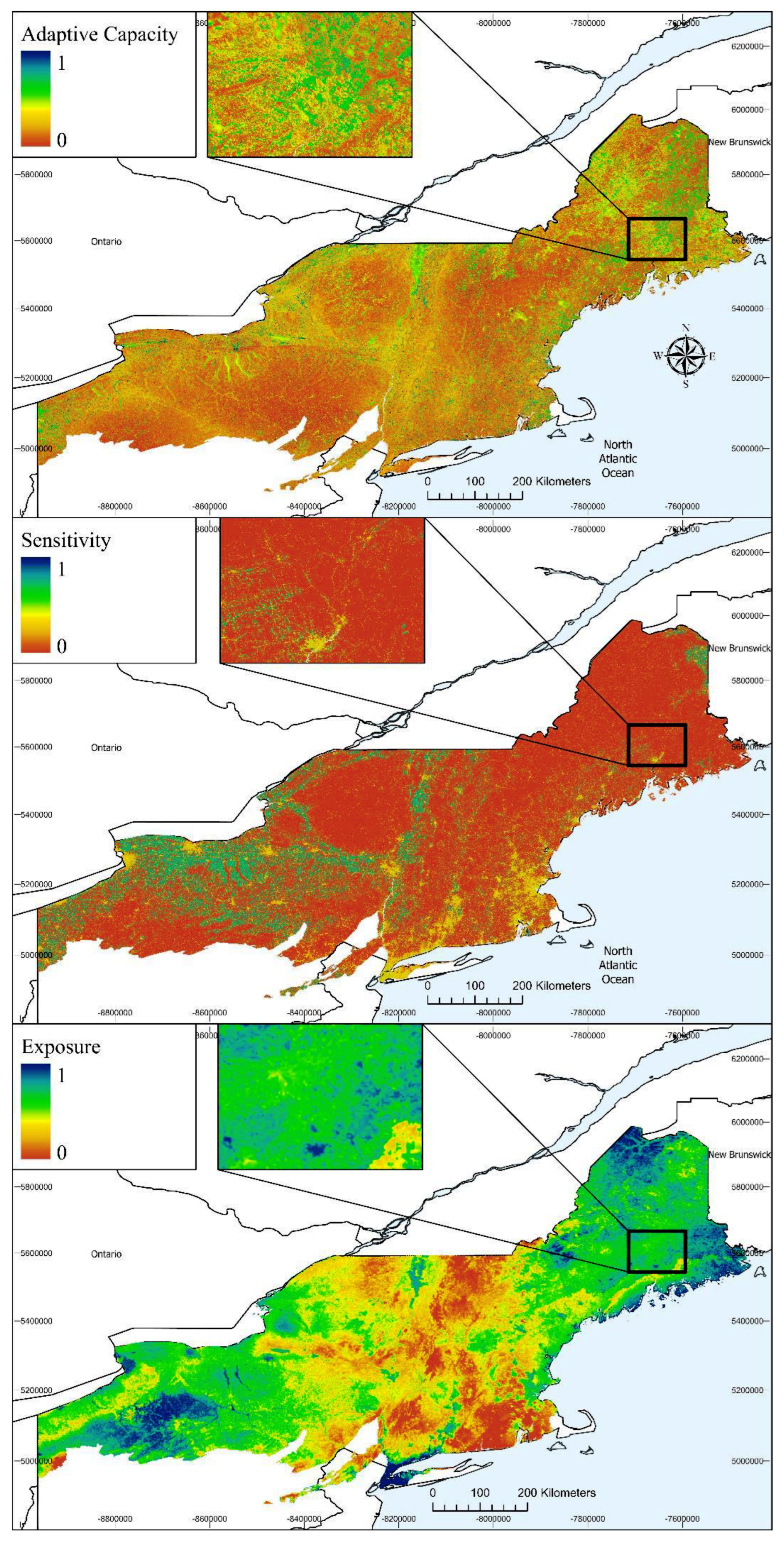
2.3. Sensitivity
2.4. Adaptive Capacity
2.5. Exposure
2.6. Geographic Distribution Data
2.7. Climate Variables
2.8. CNM Development and Evaluation
2.9. Pixel-Scale Vulnerability Calculation
2.10. Land Ownership
2.11. Landscape Suitability Model Comparison
3. Results
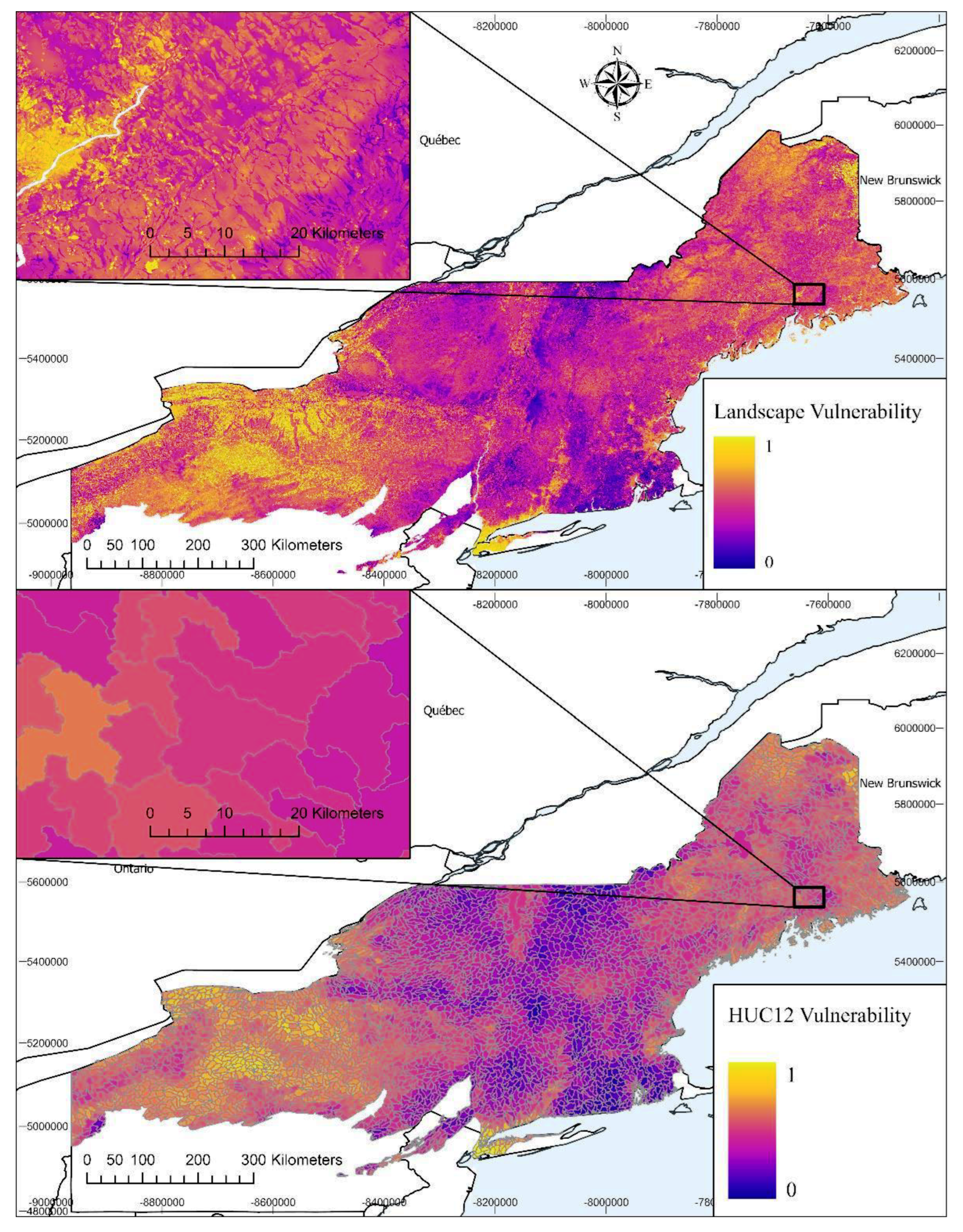
3.1. GIE and Watershed Vulnerability
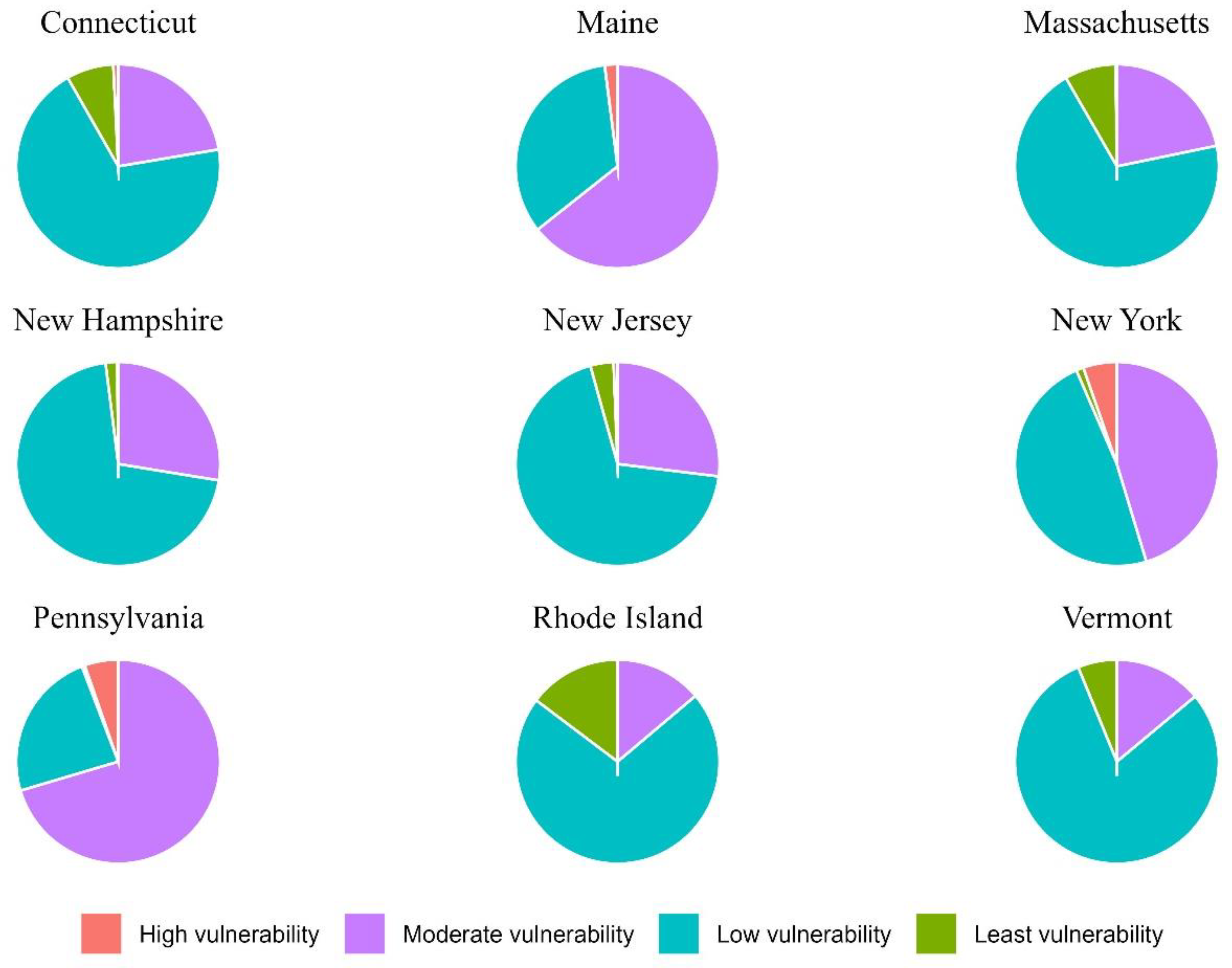
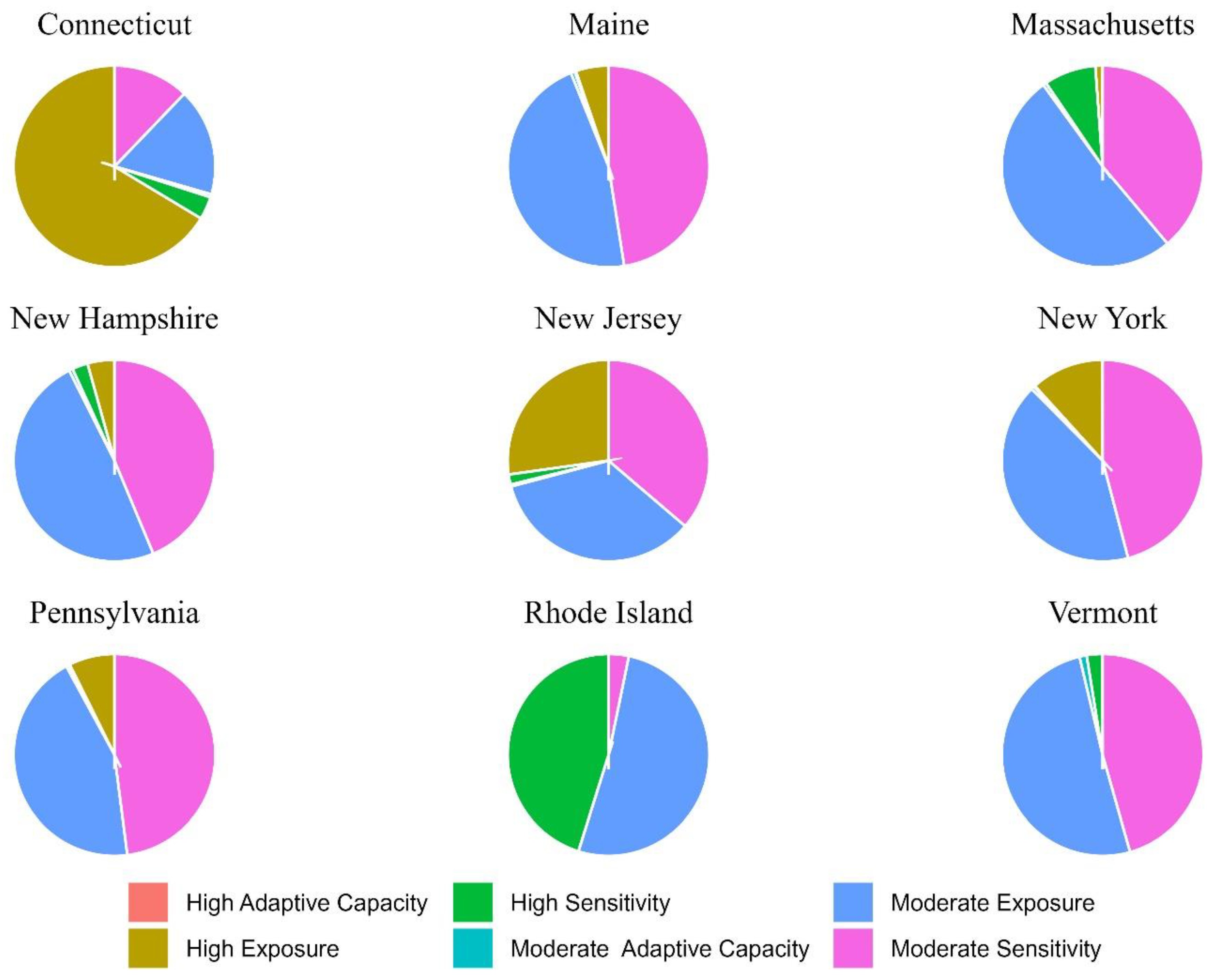
3.2. State Scale
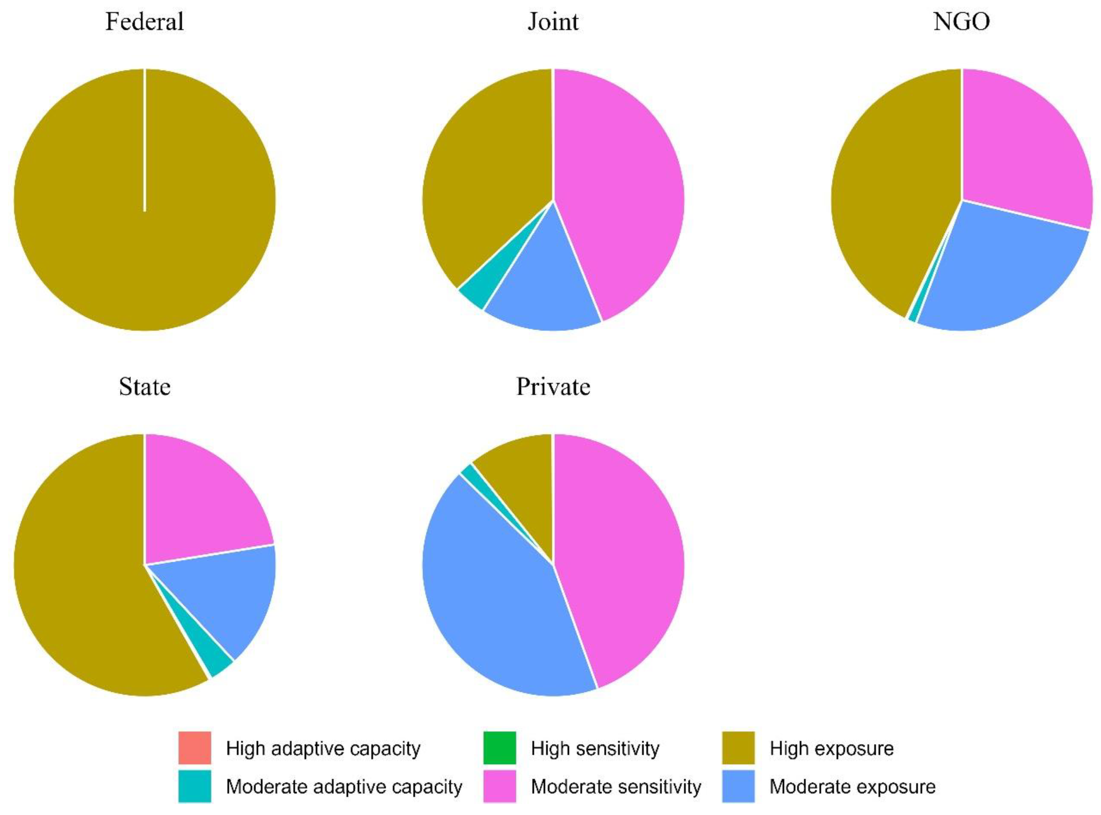
3.3. Vulnerability of Protected Areas
3.4. Climatic Niche Models
3.5. Discussion
Author Contributions
Funding
Data Availability Statement
Acknowledgments
Conflicts of Interest
References
- Lindenmayer, D.; Hobbs, R.J.; Montague-Drake, R.; Alexandra, J.; Bennett, A.; Burgman, M.; Cale, P.; Calhoun, A.; Cramer, V.; Cullen, P. A Checklist for Ecological Management of Landscapes for Conservation. Ecol. Lett. 2008, 11, 78–91. [Google Scholar] [CrossRef] [PubMed]
- Folke, C.; Carpenter, S.R.; Walker, B.; Scheffer, M.; Chapin, T.; Rockström, J. Resilience Thinking: Integrating Resilience, Adaptability and Transformability. Ecol. Soc. 2010, 15, 20. [Google Scholar] [CrossRef]
- Wurtzebach, Z.; Schultz, C. Measuring Ecological Integrity: History, Practical Applications, and Research Opportunities. BioScience 2016, 66, 446–457. [Google Scholar] [CrossRef]
- Mccallum, M. Vertebrate Biodiversity Losses Point to Sixth Mass Extiction. Biodivers. Conserv. 2015, 24, 2497–2519. [Google Scholar] [CrossRef]
- Cowie, R.H.; Bouchet, P.; Fontaine, B. The Sixth Mass Extinction: Fact, Fiction or Speculation? Biol. Rev. 2022, 97, 640–663. [Google Scholar] [CrossRef]
- Brooks, T.M.; Mittermeier, R.A.; Da Fonseca, G.A.B.; Gerlach, J.; Hoffmann, M.; Lamoreux, J.F.; Mittermeier, C.G.; Pilgrim, J.D.; Rodrigues, A.S.L. Global Biodiversity Conservation Priorities. Science 2006, 313, 58–61. [Google Scholar] [CrossRef] [PubMed]
- Wilson, K.A.; McBride, M.F.; Bode, M.; Possingham, H.P. Prioritizing Global Conservation Efforts. Nature 2006, 440, 337–340. [Google Scholar] [CrossRef]
- Dudgeon, D.; Arthington, A.H.; Gessner, M.O.; Kawabata, Z.-I.; Knowler, D.J.; Lévêque, C.; Naiman, R.J.; Prieur-Richard, A.-H.; Soto, D.; Stiassny, M.L. Freshwater Biodiversity: Importance, Threats, Status and Conservation Challenges. Biol. Rev. 2006, 81, 163–182. [Google Scholar] [CrossRef]
- Dodds, W.K.; Perkin, J.S.; Gerken, J.E. Human Impact on Freshwater Ecosystem Services: A Global Perspective. Environ. Sci. Technol. 2013, 47, 9061–9068. [Google Scholar] [CrossRef]
- Reid, A.J.; Carlson, A.K.; Creed, I.F.; Eliason, E.J.; Gell, P.A.; Johnson, P.T.J.; Kidd, K.A.; MacCormack, T.J.; Olden, J.D.; Ormerod, S.J.; et al. Emerging Threats and Persistent Conservation Challenges for Freshwater Biodiversity. Biol. Rev. 2019, 94, 849–873. [Google Scholar] [CrossRef]
- Craig, L.S.; Olden, J.D.; Arthington, A.H.; Entrekin, S.; Hawkins, C.P.; Kelly, J.J.; Kennedy, T.A.; Maitland, B.M.; Rosi, E.J.; Roy, A.H.; et al. Meeting the Challenge of Interacting Threats in Freshwater Ecosystems: A Call to Scientists and Managers. Elem. Sci. Anthr. 2017, 5, 72. [Google Scholar] [CrossRef]
- Brown, J.; Wyers, A.; Bach, L.; Aldous, A. Groundwater-Dependent Biodiversity and Associated Threats: A Statewide Screening Methodology and Spatial Assessment of Oregon. In Groundwater-Dependent Biodiversity and Associated Threats: A Statewide Screening Methodology and Spatial Assessment of Oregon; The Nature Conservancy: Arlington, VA, USA, 2009. [Google Scholar]
- Blevins, E.; Aldous, A. Biodiversity Value of Groundwater-Dependent Ecosystems. Nat. Conserv. WSP 2011, 7, 18–24. [Google Scholar]
- Rohde, M.M.; Froend, R.; Howard, J. A Global Synthesis of Managing Groundwater Dependent Ecosystems under Sustainable Groundwater Policy. Groundwater 2017, 55, 293–301. [Google Scholar] [CrossRef] [PubMed]
- Glasser, S.P. USDA Forest Service Policy on Managing Groundwater Resources. Adv. Fundam. Sci. 2007, 1, 166. [Google Scholar]
- Eamus, D. Identifying Groundwater Dependent Ecosystems: A Guide for Land and Water Managers; Land & Water Australia: Canberra, Australia, 2009. [Google Scholar]
- Hoyos, I.P.; Krakauer, N.; Khanbilvardi, R. Random Forest for Identification and Characterization of Groundwater Dependent Ecosystems. WIT Trans. Ecol. Environ. 2015, 196, 89–100. [Google Scholar]
- Fauvet, G.; Claret, C.; Marmonier, P. Influence of Benthic and Interstitial Processes on Nutrient Changes along a Regulated Reach of a Large River (Rhône River, France). Hydrobiologia 2001, 445, 121–131. [Google Scholar] [CrossRef]
- Kløve, B.; Ala-aho, P.; Bertrand, G.; Boukalova, Z.; Ertürk, A.; Goldscheider, N.; Ilmonen, J.; Karakaya, N.; Kupfersberger, H.; Kvœrner, J.; et al. Groundwater Dependent Ecosystems. Part I: Hydroecological Status and Trends. Environ. Sci. Policy 2011, 14, 770–781. [Google Scholar] [CrossRef]
- Humphreys, W.F. Hydrogeology and Groundwater Ecology: Does Each Inform the Other? Hydrogeol. J. 2009, 17, 5–21. [Google Scholar] [CrossRef]
- Brown, J.; Bach, L.; Aldous, A.; Wyers, A.; DeGagné, J. Groundwater-Dependent Ecosystems in Oregon: An Assessment of Their Distribution and Associated Threats. Front. Ecol. Environ. 2011, 9, 97–102. [Google Scholar] [CrossRef]
- Kløve, B.; Ala-Aho, P.; Bertrand, G.; Gurdak, J.J.; Kupfersberger, H.; Kværner, J.; Muotka, T.; Mykrä, H.; Preda, E.; Rossi, P.; et al. Climate Change Impacts on Groundwater and Dependent Ecosystems. J. Hydrol. 2014, 518, 250–266. [Google Scholar] [CrossRef]
- Pérez Hoyos, I.C.; Krakauer, N.Y.; Khanbilvardi, R.; Armstrong, R.A. A Review of Advances in the Identification and Characterization of Groundwater Dependent Ecosystems Using Geospatial Technologies. Geosciences 2016, 6, 17. [Google Scholar] [CrossRef]
- Condon, L.E.; Atchley, A.L.; Maxwell, R.M. Evapotranspiration Depletes Groundwater under Warming over the Contiguous United States. Nat. Commun. 2020, 11, 873. [Google Scholar] [CrossRef] [PubMed]
- Winter, T.C.; Harvey, J.W.; Franke, O.L.; Alley, W.M. US Geological Survey Circular 1139. Ground Water Surf. Water A Single Resour. 1998, 50, 2–50. [Google Scholar]
- Haynes, A.B.; Briggs, M.A.; Moore, E.; Jackson, K.; Knighton, J.; Rey, D.M.; Helton, A.M. Shallow and Local or Deep and Regional? Inferring Source Groundwater Characteristics across Mainstem Riverbank Discharge Faces. Hydrol. Process. 2023, 37, e14939. [Google Scholar] [CrossRef]
- Briggs, M.A.; Harvey, J.W.; Hurley, S.T.; Rosenberry, D.O.; McCobb, T.; Werkema, D.; Lane Jr, J.W. Hydrogeochemical Controls on Brook Trout Spawning Habitats in a Coastal Stream. Hydrol. Earth Syst. Sci. 2018, 22, 6383. [Google Scholar] [CrossRef] [PubMed]
- Ferguson, G.; Gleeson, T. Vulnerability of Coastal Aquifers to Groundwater Use and Climate Change. Nat. Clim. Change 2012, 2, 342. [Google Scholar] [CrossRef]
- Noss, R.F.; LaRoe, E.T.; Scott, J.M. Endangered Ecosystems of the United States: A Preliminary Assessment of Loss and Degradation; US Department of the Interior, National Biological Service: Washington, DC, USA, 1995; Volume 28. [Google Scholar]
- Lamptey, B.L.; Barron, E.J.; Pollard, D. Impacts of Agriculture and Urbanization on the Climate of the Northeastern United States. Glob. Planet. Chang. 2005, 49, 203–221. [Google Scholar] [CrossRef]
- Eggleston, J.; Mccoy, K. Assessing the Magnitude and Timing of Anthropogenic Warming of a Shallow Aquifer: Example from Virginia Beach, USA. Hydrogeol. J. 2014, 23, 105–120. [Google Scholar] [CrossRef]
- Kaushal, S.S.; Groffman, P.M.; Likens, G.E.; Belt, K.T.; Stack, W.P.; Kelly, V.R.; Band, L.E.; Fisher, G.T. Increased Salinization of Fresh Water in the Northeastern United States. Proc. Natl. Acad. Sci. USA 2005, 102, 13517–13520. [Google Scholar] [CrossRef]
- Climate Change 2007: Impacts, Adaptation and Vulnerability. Contribution of Working Group II to the Fourth Assessment Report of the Intergovernmental Panel on Climate Change—ProQuest. Available online: https://www.proquest.com/openview/10ac1638830c779bb315884da3366533/1?pq-origsite=gscholar&cbl=32284 (accessed on 21 April 2023).
- Magness, D.R.; Morton, J.M.; Huettmann, F.; Chapin III, F.S.; McGuire, A.D. A Climate-Change Adaptation Framework to Reduce Continental-Scale Vulnerability across Conservation Reserves. Ecosphere 2011, 2, 1–23. [Google Scholar] [CrossRef]
- Smit, B.; Wandel, J. Adaptation, Adaptive Capacity and Vulnerability. Glob. Environ. Change 2006, 16, 282–292. [Google Scholar] [CrossRef]
- Snyder, S.D.; Loftin, C.S.; Reeve, A.S. Predicting the Presence of Groundwater-Influenced Ecosystems in the Northeastern United States with Ensembled Models. Water 2023, 15, 4035. [Google Scholar] [CrossRef]
- Omernik, J.M.; Griffith, G.E. Ecoregions of the Conterminous United States: Evolution of a Hierarchical Spatial Framework. Environ. Manag. 2014, 54, 1249–1266. [Google Scholar] [CrossRef] [PubMed]
- McGarigal, K.; Compton, B.W.; Plunkett, E.B.; Grand, J. Designing Sustainable Landscapes: Development and Hard Development Settings Variables. 2020. Available online: https://umassdsl.org/data/ecological-integrity-metrics/ (accessed on 12 September 2022).
- Plunkett, E.B.; McGarigal, K.; Compton, B.W.; Jackson, S.D.; DeLuca, W.V.; Grand, J. Designing Sustainable Landscapes Products, Including Technical Documentation and Data Products. 2022. Available online: https://umassdsl.org/Data/ (accessed on 12 September 2022).
- Raney, P.A.; Leopold, D.J. Fantastic Wetlands and Where to Find Them: Modeling Rich Fen Distribution in New York State with Maxent. Wetlands 2018, 38, 81–93. [Google Scholar] [CrossRef]
- Theobald, D.M.; Harrison-Atlas, D.; Monahan, W.B.; Albano, C.M. Ecologically-Relevant Maps of Landforms and Physiographic Diversity for Climate Adaptation Planning. PLoS ONE 2015, 10, e0143619. [Google Scholar] [CrossRef] [PubMed]
- Soil Survey Staff, Natural Resources Conservation Service, United States Department of Agriculture. Soil Survey Geographic (SSURGO) Database for the Northeastern United States; United States Department of Agriculture: Washington DC, USA, 2020. [Google Scholar]
- Hijmans, R.J.; Graham, C.H. The Ability of Climate Envelope Models to Predict the Effect of Climate Change on Species Distributions. Glob. Chang. Biol. 2006, 12, 2272–2281. [Google Scholar] [CrossRef]
- Bradley, B.A.; Wilcove, D.S.; Oppenheimer, M. Climate Change Increases Risk of Plant Invasion in the Eastern United States. Biol. Invasions 2010, 12, 1855–1872. [Google Scholar] [CrossRef]
- Watling, J.I.; Romañach, S.S.; Bucklin, D.N.; Speroterra, C.; Brandt, L.A.; Pearlstine, L.G.; Mazzotti, F.J. Do Bioclimate Variables Improve Performance of Climate Envelope Models? Ecol. Model. 2012, 246, 79–85. [Google Scholar] [CrossRef]
- Fewster, R.E.; Morris, P.J.; Ivanovic, R.F.; Swindles, G.T.; Peregon, A.M.; Smith, C.J. Imminent Loss of Climate Space for Permafrost Peatlands in Europe and Western Siberia. Nat. Clim. Change 2022, 12, 373–379. [Google Scholar] [CrossRef]
- Kløve, B.; Allan, A.; Bertrand, G.; Druzynska, E.; Ertürk, A.; Goldscheider, N.; Henry, S.; Karakaya, N.; Karjalainen, T.P.; Koundouri, P.; et al. Groundwater Dependent Ecosystems. Part II. Ecosystem Services and Management in Europe under Risk of Climate Change and Land Use Intensification. Environ. Sci. Policy 2011, 14, 782–793. [Google Scholar] [CrossRef]
- Griebler, C.; Avramov, M.; Hose, G. Groundwater Ecosystems and Their Services: Current Status and Potential Risks. In Atlas of Ecosystem Services: Drivers, Risks, and Societal Responses; Schröter, M., Bonn, A., Klotz, S., Seppelt, R., Baessler, C., Eds.; Springer International Publishing: Cham, Switzerland, 2019; pp. 197–203. ISBN 978-3-319-96229-0. [Google Scholar]
- Thornton, M.M.; Shrestha, R.; Wei, Y.; Thornton, P.E.; Kao, S.-C.; Wilson, B.E. Daymet: Daily Surface Weather Data on a 1-Km Grid for North America, Version 4 R1 2020. Available online: https://daac.ornl.gov/DAYMET/guides/Daymet_Daily_V4.html (accessed on 20 January 2023).
- Hijmans, R.J.; Phillips, S.; Leathwick, J.; Elith, J. Dismo: Species Distribution Modeling; R Package Version 1.0-12; The R Foundation for Statistical Computing: Vienna, Austria, 2015. [Google Scholar]
- Gorelick, N.; Hancher, M.; Dixon, M.; Ilyushchenko, S.; Thau, D.; Moore, R. Google Earth Engine: Planetary-Scale Geospatial Analysis for Everyone. Remote Sens. Environ. 2017, 202, 18–27. [Google Scholar] [CrossRef]
- Jeschke, J.M.; Strayer, D.L. Usefulness of Bioclimatic Models for Studying Climate Change and Invasive Species. Ann. N. Y. Acad. Sci. 2008, 1134, 1–24. [Google Scholar] [CrossRef] [PubMed]
- Zhang, K.; Zhang, Y.; Tao, J. Predicting the Potential Distribution of Paeonia Veitchii (Paeoniaceae) in China by Incorporating Climate Change into a Maxent Model. Forests 2019, 10, 190. [Google Scholar] [CrossRef]
- Kiraç, A. Potential Distribution of Two Lynx Species in Europe under Paleoclimatological Scenarios and Anthropogenic Climate Change Scenarios. Cerne 2021, 27, e102517. [Google Scholar] [CrossRef]
- Qiao, H.; Soberón, J.; Peterson, A.T. No Silver Bullets in Correlative Ecological Niche Modelling: Insights from Testing among Many Potential Algorithms for Niche Estimation. Methods Ecol. Evol. 2015, 6, 1126–1136. [Google Scholar] [CrossRef]
- Phillips, S.J.; Anderson, R.P.; Schapire, R.E. Maximum Entropy Modeling of Species Geographic Distributions. Ecol. Model. 2006, 190, 231–259. [Google Scholar] [CrossRef]
- Wood, S.N. Fast Stable Restricted Maximum Likelihood and Marginal Likelihood Estimation of Semiparametric Generalized Linear Models: Estimation of Semiparametric Generalized Linear Models. J. R. Stat. Soc. Ser. B (Stat. Methodol.) 2011, 73, 3–36. [Google Scholar] [CrossRef]
- Baldwin, R.A. Use of Maximum Entropy Modeling in Wildlife Research. Entropy 2009, 11, 854–866. [Google Scholar] [CrossRef]
- Viera, A.J.; Garrett, J.M. Understanding Interobserver Agreement: The Kappa Statistic. Fam. Med. 2015, 37, 360–363. [Google Scholar]
- Allouche, O.; Tsoar, A.; Kadmon, R. Assessing the Accuracy of Species Distribution Models: Prevalence, Kappa and the True Skill Statistic (TSS). J. Appl. Ecol. 2006, 43, 1223–1232. [Google Scholar] [CrossRef]
- McElfish, J.M.; Kihslinger, R.L.; Nichols, S. Setting Buffer Sizes for Wetlands. Natl. Wetl. Newsl. 2008, 30, 6–17. [Google Scholar]
- Marczak, L.B.; Sakamaki, T.; Turvey, S.L.; Deguise, I.; Wood, S.L.R.; Richardson, J.S. Are Forested Buffers an Effective Conservation Strategy for Riparian Fauna? An Assessment Using Meta-Analysis. Ecol. Appl. 2010, 20, 126–134. [Google Scholar] [CrossRef] [PubMed]
- Allan, D.; Erickson, D.; Fay, J. The Influence of Catchment Land Use on Stream Integrity across Multiple Spatial Scales. Freshw. Biol. 1997, 37, 149–161. [Google Scholar] [CrossRef]
- Schiff, R.; Benoit, G. Effects of Impervious Cover at Multiple Spatial Scales on Coastal Watershed Streams1. JAWRA J. Am. Water Resour. Assoc. 2007, 43, 712–730. [Google Scholar] [CrossRef]
- Shi, P.; Zhang, Y.; Li, Z.; Li, P.; Xu, G. Influence of Land Use and Land Cover Patterns on Seasonal Water Quality at Multi-Spatial Scales. Catena 2017, 151, 182–190. [Google Scholar] [CrossRef]
- Shu, X.; Wang, W.; Zhu, M.; Xu, J.; Tan, X.; Zhang, Q. Impacts of Land Use and Landscape Pattern on Water Quality at Multiple Spatial Scales in a Subtropical Large River. Ecohydrology 2022, 15, e2398. [Google Scholar] [CrossRef]
- Karmalkar, A.V.; Bradley, R.S. Consequences of Global Warming of 1.5 °C and 2 °C for Regional Temperature and Precipitation Changes in the Contiguous United States. PLoS ONE 2017, 12, e0168697. [Google Scholar] [CrossRef]
- Fernandez, I.J.; Birkel, S.; Simonson, J.; Lyon, B.; Pershing, A.; Stancioff, E.; Jacobson, G.L.; Mayewski, P.A. Maine’s Climate Future: 2020 Update. 2020. Available online: https://digitalcommons.library.umaine.edu/cgi/viewcontent.cgi?article=1005&context=climate_facpub (accessed on 10 March 2023).
- Notaro, M.; Lorenz, D.; Hoving, C.; Schummer, M. Twenty-First-Century Projections of Snowfall and Winter Severity across Central-Eastern North America. J. Clim. 2014, 27, 6526–6550. [Google Scholar] [CrossRef]
- Melillo, J.M.; Richmond, T.; Yohe, G.W. Climate Change Impacts in the United States: The Third National Climate Assessment; U.S. Global Change Research Program: Washington, DC, USA, 2014. [Google Scholar]
- Karl, T.R.; Meehl, G.A.; Miller, C.D.; Hassol, S.J.; Waple, A.M.; Murray, W.L. Weather and Climate Extremes in a Changing Climate; US Climate Change Science Program: Washington, DC, USA, 2008. [Google Scholar]
- Brookfield, A.E.; Macpherson, G.L.; Covington, M.D. Effects of Changing Meteoric Precipitation Patterns on Groundwater Temperature in Karst Environments. Groundwater 2017, 55, 227–236. [Google Scholar] [CrossRef]
- Thomas, B.F.; Behrangi, A.; Famiglietti, J.S. Precipitation Intensity Effects on Groundwater Recharge in the Southwestern United States. Water 2016, 8, 90. [Google Scholar] [CrossRef]
- Wang, H.; Stephenson, S.R. Quantifying the Impacts of Climate Change and Land Use/Cover Change on Runoff in the Lower Connecticut River Basin. Hydrol. Process. 2018, 32, 1301–1312. [Google Scholar] [CrossRef]
- Santos, M.J.; Smith, A.B.; Dekker, S.C.; Eppinga, M.B.; Leitão, P.J.; Moreno-Mateos, D.; Morueta-Holme, N.; Ruggeri, M. The Role of Land Use and Land Cover Change in Climate Change Vulnerability Assessments of Biodiversity: A Systematic Review. Landsc. Ecol 2021, 36, 3367–3382. [Google Scholar] [CrossRef]
- Potter, K.; Douglas, J.; Bricj, E.; DeFries, R.S.; Asner, G.P.; Houghton, R.A. Impacts of Agriculture on Aquatic Ecosystems in the Humid United States. Ecosyst. Land Use Change Am. Geophys. Union 2004, 153, 31–40. [Google Scholar]
- Bai, Y.; Ochuodho, T.O.; Yang, J. Impact of Land Use and Climate Change on Water-Related Ecosystem Services in Kentucky, USA. Ecol. Indic. 2019, 102, 51–64. [Google Scholar] [CrossRef]
- Pham, H.V.; Sperotto, A.; Torresan, S.; Acuña, V.; Jorda-Capdevila, D.; Rianna, G.; Marcomini, A.; Critto, A. Coupling Scenarios of Climate and Land-Use Change with Assessments of Potential Ecosystem Services at the River Basin Scale. Ecosyst. Serv. 2019, 40, 101045. [Google Scholar] [CrossRef]
- Vaighan, A.A.; Talebbeydokhti, N.; Bavani, A.M. Assessing the Impacts of Climate and Land Use Change on Streamflow, Water Quality and Suspended Sediment in the Kor River Basin, Southwest of Iran. Env. Earth Sci. 2017, 76, 543. [Google Scholar] [CrossRef]
- Serov, P.; Kuginis, L.; Williams, J.P. Risk Assessment Guidelines for Groundwater Dependent Ecosystems, Volume 1—The Conceptual Framework; NSW Department of Primary Industries, Office of Water: Sydney, Australia, 2012. [Google Scholar]
- Keiter, R.B. Toward a National Conservation Network Act: Transforming Landscape Conservation on the Public Lands into Law. SSRN J. 2018, 42, 61. [Google Scholar] [CrossRef]
- Li, P.; Wu, J. Sustainable Living with Risks: Meeting the Challenges. Hum. Ecol. Risk Assess. Int. J. 2019, 25, 1–10. [Google Scholar] [CrossRef]
- Li, P. To Make the Water Safer. Expo Health 2020, 12, 337–342. [Google Scholar] [CrossRef]
- Beier, P.; Hunter, M.L.; Anderson, M. Conserving Nature’s Stage. Conserv. Biol. J. Soc. Conserv. Biol. 2015, 29, 613–617. [Google Scholar] [CrossRef]
- Hao, R.; Yu, D.; Liu, Y.; Liu, Y.; Qiao, J.; Wang, X.; Du, J. Impacts of Changes in Climate and Landscape Pattern on Ecosystem Services. Sci. Total Environ. 2017, 579, 718–728. [Google Scholar] [CrossRef]
- Côté, I.M.; Darling, E.S. Rethinking Ecosystem Resilience in the Face of Climate Change. PLoS Biol. 2010, 8, e1000438. [Google Scholar] [CrossRef] [PubMed]
- Olds, A.D.; Pitt, K.A.; Maxwell, P.S.; Connolly, R.M. Synergistic Effects of Reserves and Connectivity on Ecological Resilience. J. Appl. Ecol. 2012, 49, 1195–1203. [Google Scholar] [CrossRef]
- Mumby, P.J.; Chollett, I.; Bozec, Y.-M.; Wolff, N.H. Ecological Resilience, Robustness and Vulnerability: How Do These Concepts Benefit Ecosystem Management? Curr. Opin. Environ. Sustain. 2014, 7, 22–27. [Google Scholar] [CrossRef]
- Snyder, S.D.; Loftin, C.S.; Reeve, A.S. Vulnerability of Groundwater Influenced Ecosystems in the Northeastern United States: U.S. Geological Survey Data Release. 2024. Available online: https://www.sciencebase.gov/catalog/item/660ab004d34e4df16bd5898f (accessed on 10 March 2023).


| Category | Data | Variables | Source |
|---|---|---|---|
| Exposure | tmin, tmax, prcp | Bio1, 3, 9, 10, 12, 14, 18 | https://daymet.ornl.gov/ |
| Evapotranspiration | ET, PET, ET-GS | https://lpdaac.usgs.gov/products/mod16a2gfv006/ | |
| Adaptive capacity | Topographic Wetness Index (TWI) | TWI | https://umassdsl.org/data/ecological-settings/ |
| Physiographic Diversity | Physiographic diversity | https://developers.google.com/earth-engine/datasets/catalog/CSP_ERGo_1_0_US_physioDiversity | |
| Hydric Soil | Percent hydric soil | https://www.nrcs.usda.gov/resources/data-and-reports/gridded-soil-survey-geographic-gssurgo-database | |
| Sensitivity | Agriculture Land Cover | Percent agriculture land | https://www.mrlc.gov/data/nlcd-2019-land-cover-conus |
| Developed Land Cover | Percent developed land | https://www.mrlc.gov/data/nlcd-2019-land-cover-conus | |
| Aquatic Barriers | Aquatic barriers | https://umassdsl.org/data/ecological-settings/ |
| Vulnerability Categories | Square Kilometers | Percent of Ecoregion | GIE Area (km2) | Percent of Total GIE Area |
|---|---|---|---|---|
| 0 ≤ value < 0.25 | 4836 | 1.5 | 1212 | 19.6 |
| 0.25 ≤ value < 0.50 | 203,236 | 63.2 | 4308 | 69.5 |
| 0.50 ≤ value ≤ 0.75 | 105,787 | 32.9 | 669 | 10.8 |
| 0.75 < value ≤ 1 | 7728 | 2.4 | 11 | 0.2 |
| Number of HUC12 Watersheds | Percent of Watersheds | GIE Area (km2) | Percent of Total GIE Area | |
| 0 ≤ value < 0.25 | 0.25 | 0.6 | 34.92 | 0.5 |
| 0.25 ≤ value < 0.50 | 19 | 44.5 | 5633 | 80.5 |
| 0.50 ≤ value ≤ 0.75 | 23 | 54.6 | 1329 | 19.0 |
| 0.75 < value ≤ 1 | 0.14 | 0.3 | 0 | 0.0 |
| Vulnerability Score | GIEs Counts | Percent of GIEs | GIE Area (km2) | Percent of Total GIE Area |
|---|---|---|---|---|
| <0.25 | 13,847 | 4.8 | 361 | 5 |
| <0.50 | 196,795 | 67.9 | 5045 | 68.1 |
| ≥0.50 | 77,344 | 26.7 | 1952 | 26.4 |
| ≥0.75 | 1878 | 0.6 | 45 | 0.6 |
| Number of GIEs | |||||
|---|---|---|---|---|---|
| Exposure | Exposure | Sensitivity | Sensitivity | ||
| ≥0.50 | ≥0.75 | ≥0.50 | ≥0.75 | ||
| Exposure | ≥0.50 | 31,563 | - | 5837 | 177 |
| Exposure | ≥0.75 | - | 774 | 185 | 3 |
| Sensitivity | ≥0.50 | 5837 | 185 | 14,419 | - |
| Sensitivity | ≥0.75 | 177 | 3 | - | 460 |
| Percent of Vulnerable GIE area | |||||
| Exposure | Exposure | Sensitivity | Sensitivity | ||
| ≥0.50 | ≥0.75 | ≥0.50 | ≥0.75 | ||
| Exposure | ≥0.50 | 40.8 | - | 7.5 | 0.2 |
| Exposure | ≥0.75 | - | 1.0 | 0.2 | <0.01 |
| Sensitivity | ≥0.50 | 7.5 | 0.2 | 18.6 | - |
| Sensitivity | ≥0.75 | 0.2 | <0.01 | - | 0.6 |
| Distance Band (m) | Number of GIEs in Distance Band | Percent of Total GIEs | GIE Area (km2) in Distance Band | Percent of GIE Area |
|---|---|---|---|---|
| <50 | 1628 | 0.6 | 56 | 0.8 |
| <100 | 2581 | 0.9 | 78 | 1.1 |
| <200 | 4049 | 1.5 | 109 | 1.6 |
| <300 | 5243 | 1.9 | 127 | 1.8 |
| <400 | 6277 | 2.3 | 139 | 2.0 |
| <800 | 9599 | 3.5 | 177 | 2.5 |
| Vulnerability Score | <0.25 | <0.25 | <0.50 | <0.50 | ≥0.50 | ≥0.50 | ≥0.75 | ≥0.75 |
|---|---|---|---|---|---|---|---|---|
| State | Area (km2) | Percent of State | Area (km2) | Percent of State | Area (km2) | Percent of State | Area (km2) | Percent of State |
| Connecticut | 1374 | 8.0 | 12,743 | 74.1 | 4104 | 23.9 | 143 | 0.8 |
| Maine | 46 | 0.0 | 39,941 | 33.8 | 76,437 | 64.7 | 2383 | 2.0 |
| Massachusetts 1 | 2248 | 7.9 | 19,259 | 67.5 | 5995 | 21.0 | 46 | 0.2 |
| New Hampshire | 623 | 1.9 | 23,685 | 71.6 | 9271 | 28.0 | 49 | 0.2 |
| New Jersey 1 | 107 | 0.4 | 2003 | 7.9 | 785 | 3.1 | 18 | 0.1 |
| New York 1 | 2057 | 1.2 | 84,188 | 49.1 | 79,204 | 46.2 | 9316 | 5.4 |
| Pennsylvania 1 | 291 | 0.2 | 14,427 | 9.3 | 42,737 | 27.6 | 3238 | 2.1 |
| Rhode Island | 586 | 16.2 | 2845 | 78.7 | 551 | 15.3 | 0.20 | 0.0 |
| Vermont | 2251 | 6.5 | 29,225 | 84.7 | 5101 | 14.8 | 15 | 0.0 |
| Vulnerability Score | <0.25 | <0.25 | <0.25 | <0.50 | <0.50 | <0.50 | ≥0.50 | ≥0.50 | ≥0.50 | ≥0.75 | ≥0.75 | ≥0.75 |
|---|---|---|---|---|---|---|---|---|---|---|---|---|
| State | Number of Watersheds | Area (km2) | Percent of State | Number of Watersheds | Area (km2) | Percent of State | Number of Watersheds | Area (km2) | Percent of State | Number of Watersheds | Area (km2) | Percent of State |
| Connecticut | 0 | 0 | 0 | 154 | 14,049 | 81.7 | 30 | 2937 | 17.1 | 0 | 0 | 0 |
| Maine | 0 | 0 | 0 | 230 | 27,412 | 23.2 | 831 | 8998 | 76.1 | 0 | 0 | 0 |
| Massachusetts 1 | 0 | 0 | 0 | 215 | 22,341 | 78.3 | 38 | 3176 | 11.1 | 0 | 0 | 0 |
| New Hampshire | 0 | 0 | 0 | 299 | 29,221 | 88.4 | 44 | 3790 | 11.5 | 0 | 0 | 0 |
| New Jersey 1 | 0 | 0 | 0 | 39 | 2161 | 8.5 | 17 | 749 | 2.9 | 2 | 24 | 0.1 |
| New York 1 | 0 | 0 | 0 | 721 | 76,597 | 44.7 | 911 | 87,526 | 51.1 | 14 | 798 | 0.5 |
| Pennsylvania 1 | 0 | 0 | 0 | 111 | 8049 | 5.2 | 517 | 49,456 | 31.9 | 0 | 0 | 0 |
| Rhode Island | 0 | 0 | 0 | 56 | 3319 | 91.8 | 2 | 187 | 5.2 | 0 | 0 | 0 |
| Vermont | 1 | 287 | 0.008 | 253 | 31,794 | 92.1 | 15 | 2711 | 7.9 | 0 | 0 | 0 |
| km2 | ||||||||||
|---|---|---|---|---|---|---|---|---|---|---|
| CT | ME | MA | NH | NJ | NY | PA | RI | VT | ||
| Exposure | High | 105 | 237 | 1 | 4 | 8 | 2025 | 454 | 0 | 0.02 |
| Moderate | 27 | 2096 | 41 | 42 | 10 | 7195 | 2738 | 0.2 | 15 | |
| Adaptive Capacity | High | 0.02 | 1 | 0.02 | 0.01 | 0.003 | 2 | 1 | 0 | 0 |
| Moderate | 1 | 28 | 0.4 | 1 | 0.1 | 86 | 30 | 0 | 0.3 | |
| Sensitivity | High | 6 | 10 | 7 | 2 | 0.5 | 32 | 7 | 0.1 | 1 |
| Moderate | 19 | 2146 | 31 | 38 | 10 | 7931 | 2976 | 0.01 | 13 | |
| Percent | ||||||||||
| Exposure | High | 73.3 | 10.0 | 2.0 | 7.4 | 42.5 | 21.7 | 14.0 | 0 | 0.1 |
| Moderate | 19.1 | 87.9 | 87.3 | 84.0 | 54.0 | 77.2 | 84.5 | 80.9 | 95.6 | |
| Adaptive Capacity | High | 0.01 | 0.02 | 0.03 | 0.02 | 0 | 0.02 | 0.03 | 0 | 0 |
| Moderate | 0.5 | 1.2 | 0.9 | 1.0 | 0.5 | 0.9 | 0.9 | 0.3 | 2.2 | |
| Sensitivity | High | 4.0 | 0.4 | 14.2 | 4.3 | 2.5 | 0.3 | 0.2 | 69.6 | 4.7 |
| Moderate | 13.4 | 90.0 | 66.4 | 75.1 | 56.6 | 85.1 | 91.9 | 6.4 | 86.0 |
| Vulnerability Score | <0.25 | <0.25 | <0.50 | <0.50 | ≥0.50 | ≥0.50 | ≥0.75 | ≥0.75 |
|---|---|---|---|---|---|---|---|---|
| Ownership Type | Area (km2) | Percent of Ownership Type | Area (km2) | Percent of Ownership Type | Area (km2) | Percent of Ownership Type | Area (km2) | Percent of Ownership Type |
| Federal | 266 | 2.3 | 6835 | 59.3 | 4640 | 40.3 | 33 | 0.3 |
| Joint | 0.73 | 0.0 | 1001 | 25.7 | 2862 | 73.5 | 23 | 0.6 |
| Non-Governmental Organization | 244 | 4.0 | 3469 | 57.1 | 2510 | 42.3 | 10 | 0.2 |
| Private | 376 | 2.0 | 9280 | 49.7 | 9188 | 49.2 | 65 | 0.4 |
| State | 1027 | 2.1 | 30,236 | 60.7 | 19,269 | 38.7 | 86 | 0.2 |
| Mean Vulnerability Score < 0.25 | Mean Vulnerability Score < 0.50 | Mean Vulnerability Score ≥ 0.50 | Mean Vulnerability Score ≥ 0.75 | ||
|---|---|---|---|---|---|
| Management Type | Number of Protected Areas | Number of Protected Areas | Number of Protected Areas | Number of Protected Areas | Number of Protected Areas |
| Biodiversity, disturbance (1) | 1527 | 52 | 1152 | 303 | 1 |
| Biodiversity, no disturbance (2) | 9602 | 506 | 6906 | 2239 | 18 |
| Multiple uses (3) | 25,205 | 1432 | 18,874 | 5106 | 75 |
| No mandate for biodiversity (4) | 31,780 | 977 | 17,003 | 12,579 | 206 |
| Total | 68,114 | 2967 | 43,935 | 20,227 | 300 |
| Proportion | Proportion | Proportion | Proportion | Proportion | |
| Biodiversity, disturbance (1) | 0.02 | 0.02 | 0.03 | 0.01 | 0.003 |
| Biodiversity, no disturbance (2) | 0.14 | 0.17 | 0.16 | 0.11 | 0.06 |
| Multiple uses (3) | 0.37 | 0.48 | 0.43 | 0.25 | 0.25 |
| No mandate for biodiversity (4) | 0.47 | 0.33 | 0.39 | 0.62 | 0.69 |
| Moderate Vulnerability | Moderate Vulnerability | High Vulnerability | High Vulnerability | |||
|---|---|---|---|---|---|---|
| Management Type | GIE Area | Percent of Total GIE Area | GIE Area | Percent of Total GIE Area | Total GIE Area | Percent of Total GIE Area |
| Biodiversity, disturbance (1) | 761 | 0.11 | 0 | 0 | 4611 | 0.7 |
| Biodiversity, no disturbance (2) | 1566 | 0.22 | 0 | 0 | 47,652 | 6.8 |
| Multiple uses (3) | 2305 | 0.33 | 1 | <0.0001 | 53,536 | 7.7 |
| No mandate for biodiversity (4) | 1720 | 0.25 | 1 | <0.0001 | 17,562 | 2.5 |
| Percent of Total | Percent of Total | Percent of Total | Percent of Total | Hectares | Hectares | Hectares | Hectares | |
|---|---|---|---|---|---|---|---|---|
| Management Type | 1 | 2 | 3 | 4 | 1 | 2 | 3 | 4 |
| High adaptive capacity | 0 | 0.02 | 0 | 0.2 | 0 | 0.02 | 0 | 3 |
| Moderate adaptive capacity | 0 | 5.5 | 3.6 | 6.0 | 0 | 7 | 1 | 83 |
| High sensitivity | 0 | 0 | 0 | 0.13 | 0 | 0 | 0 | 2 |
| Moderate sensitivity | 76.7 | 50.6 | 44.2 | 94.4 | 8 | 64 | 11 | 1298 |
| High exposure | 91.2 | 72.1 | 96.7 | 71.3 | 9 | 91 | 23 | 980 |
| Moderate exposure | 0 | 32.2 | 7.4 | 55.1 | 0 | 40 | 2 | 757 |
| Hectares | |||||
|---|---|---|---|---|---|
| Variables | Federal | Joint | NGO | Private | State |
| High adaptive capacity | 0 | 1 | 0 | 2 | 0 |
| Moderate adaptive capacity | 0 | 41 | 2 | 33 | 14 |
| High sensitivity | 0 | 0 | 0.3 | 0.4 | 1 |
| Moderate sensitivity | 0 | 453 | 53 | 784 | 90 |
| High exposure | 0.4 | 380 | 80 | 188 | 232 |
| Moderate exposure | 0 | 156 | 50 | 754 | 62 |
| Percent of area | |||||
| High adaptive capacity | 0 | 0.2 | 0 | 0.2 | 0 |
| Moderate adaptive capacity | 0 | 8.2 | 2.3 | 4.1 | 5.5 |
| High sensitivity | 0 | 0.0 | 0.3 | 0.1 | 0.4 |
| Moderate sensitivity | 0 | 90.0 | 56.6 | 97.5 | 35.4 |
| High exposure | 21.9 | 75.5 | 84.6 | 23.4 | 91.7 |
| Moderate exposure | 0 | 30.9 | 53.2 | 93.8 | 24.5 |
| Model | AUC | TSS | Kappa | Sensitivity | Specificity |
|---|---|---|---|---|---|
| Maxent | 0.77 | 0.39 | 0.18 | 0.69 | 0.77 |
| GAM | 0.76 | 0.4 | 0.17 | 0.68 | 0.76 |
| Maxent | Maxent | GAM | GAM | |
|---|---|---|---|---|
| Variables | Pearson Correlation | AUC | Pearson Correlation | AUC |
| Annual ET 1 | 12.5 | 5.2 | 10.9 | 4.6 |
| Growing Season ET 1 | 2.2 | 0.8 | 5.6 | 2.7 |
| Annual PET 2 | 24.3 | 8.6 | 21.8 | 10.5 |
| Snow–water equivalency | 24.6 | 11.3 | 12.4 | 5.8 |
| Annual mean temperature | 15.8 | 9.3 | 76.3 | 34.9 |
| Isothermality | 12.2 | 5.1 | 6.8 | 3.3 |
| Mean temperature of driest quarter | 30.2 | 16.4 | 49.0 | 18.6 |
| Mean temperature of warmest quarter | 7.9 | 3.9 | 53.5 | 27.3 |
| Annual precipitation | 52.7 | 25.3 | 64.3 | 30.0 |
| Precipitation of driest month | 49.8 | 22.6 | 81.7 | 38.2 |
| Precipitation of warmest quarter | 74.7 | 35.4 | 81.0 | 38.8 |
Disclaimer/Publisher’s Note: The statements, opinions and data contained in all publications are solely those of the individual author(s) and contributor(s) and not of MDPI and/or the editor(s). MDPI and/or the editor(s) disclaim responsibility for any injury to people or property resulting from any ideas, methods, instructions or products referred to in the content. |
© 2024 by the authors. Licensee MDPI, Basel, Switzerland. This article is an open access article distributed under the terms and conditions of the Creative Commons Attribution (CC BY) license (https://creativecommons.org/licenses/by/4.0/).
Share and Cite
Snyder, S.D.; Loftin, C.S.; Reeve, A.S. Vulnerability Assessment of Groundwater Influenced Ecosystems in the Northeastern United States. Water 2024, 16, 1366. https://doi.org/10.3390/w16101366
Snyder SD, Loftin CS, Reeve AS. Vulnerability Assessment of Groundwater Influenced Ecosystems in the Northeastern United States. Water. 2024; 16(10):1366. https://doi.org/10.3390/w16101366
Chicago/Turabian StyleSnyder, Shawn D., Cynthia S. Loftin, and Andrew S. Reeve. 2024. "Vulnerability Assessment of Groundwater Influenced Ecosystems in the Northeastern United States" Water 16, no. 10: 1366. https://doi.org/10.3390/w16101366
APA StyleSnyder, S. D., Loftin, C. S., & Reeve, A. S. (2024). Vulnerability Assessment of Groundwater Influenced Ecosystems in the Northeastern United States. Water, 16(10), 1366. https://doi.org/10.3390/w16101366