Article

Application of Oversampling Techniques for Enhanced Transverse Dispersion Coefficient Estimation Performance Using Machine Learning Regression

Department of Civil Engineering, Seoul National University of Science and Technology, 232 Gongreung-ro, Nowon-Gu, Seoul 01811, Republic of Korea
*
Author to whom correspondence should be addressed.
Water 2024, 16(10), 1359; https://doi.org/10.3390/w16101359
Submission received: 24 March 2024 / Revised: 7 May 2024 / Accepted: 9 May 2024 / Published: 10 May 2024
(This article belongs to the Special Issue Contaminant Transport Modeling in Aquatic Environments)

Abstract

:
The advection–dispersion equation has been widely used to analyze the intermediate field mixing of pollutants in natural streams. The dispersion coefficient, manipulating the dispersion term of the advection–dispersion equation, is a crucial parameter in predicting the transport distance and contaminated area in the water body. In this study, the transverse dispersion coefficient was estimated using machine learning regression methods applied to oversampled datasets. Previous research datasets used for this estimation were biased toward width-to-depth ratio ( W / H ) values ≤ 50, potentially leading to inaccuracies in estimating the transverse dispersion coefficient for datasets with W / H > 50. To address this issue, four oversampling techniques were employed to augment the dataset with W / H > 50, thereby mitigating the dataset’s imbalance. The estimation results obtained from data resampling with nonlinear regression method demonstrated improved prediction accuracy compared to the pre-oversampling results. Notably, the combination of adaptive synthetic sampling (ADASYN) and eXtreme Gradient Boosting regression (XGBoost) exhibited improved accuracy compared to other combinations of oversampling techniques and nonlinear regression methods. Through the combined ADASYN–XGBoost approach, it is possible to enhance the transverse dispersion coefficient estimation performance using only two variables, W / H and bed friction effects ( U / U * ), without adding channel sinuosity; this represents the effects of secondary currents.

1. Introduction

Water quality management is a significant task for public health and aquatic environments. The mixing stages of introduced polluted water in natural rivers are classified into three processes: near-, intermediate-, and far-field mixing. In near-field mixing, longitudinal, transverse, and vertical mixing simultaneously occur by turbulent and molecular diffusion. After finishing the vertical mixing, intermediate-field mixing begins with longitudinal and transverse dispersion. Intermediate-field mixing persists over significantly longer distances than near-field mixing due to the complex flow structures accompanying the delays in transverse mixing completion, which are caused by the irregular channel geometries [1]. In those mixing processes, the advection–dispersion equation has been used for the analysis of polluted water mixing in aquatic environments, such as rivers, lakes, and water conveyance channels. In particular, in intermediate-field mixing, following the completion of vertical mixing, the depth-averaged two-dimensional advection–dispersion equation (2D ADE) has been widely used [2,3,4,5]. The 2D ADE is defined as follows:
𝜕 C 𝜕 t + u 𝜕 C 𝜕 x + v 𝜕 C 𝜕 y = D L 𝜕 2 C 𝜕 x 2 + D T 𝜕 2 C 𝜕 y 2
where C is the depth-averaged concentration; u , v are the depth-averaged longitudinal and transverse velocities, respectively; D L , D T represent the longitudinal and transverse dispersion coefficients, respectively. From the 2D ADE, mixing behaviors, such as the arrival time of polluted water, the concentration change, and the polluted area over longitudinal and transverse distances, can be predicted by the appropriate determinations of D L and D T . D T is particularly significant in analyzing lateral mixing of polluted water caused by accidentally spilled pollutants, suspended solids, and continuous sources from tributaries and wastewater treatment effluents.
Tracer tests have been conducted to estimate D T for laboratory channels [1,6,7,8] and natural rivers [9,10,11,12]. However, the tracer test is a labor-intensive and costly experiment, and tracer materials input is limited for natural streams, especially in large-scale rivers [13]. Thus, practically, empirical formulas have been used to estimate D T using hydraulic (velocity magnitude, shear velocity, and Froude number) and geometrical (depth, width, radius of curvature, and sinuosity) parameters. Fischer et al. [14] defined that D T is proportional to H U * , where H is the flow depth and U * is the shear velocity; they suggested a proportional constant of 0.15 for straight channels and one of 0.6 for meandering channels. Rutherford [15] presented the range of the proportional constant according to the geometrical properties of rivers, where 0.15–0.3 could be used in straight channels, and 0.3–0.9 could be used in meandering channels. For expanding applicability, the empirical formulas were developed by conducting multiple linear regression using tracer test results [10,16,17,18,19,20]. The accuracy of estimated D T from the proposed empirical formulas depends on the diversity of data reflecting various hydraulic conditions that influence transverse mixing, which are used to develop the formula. In other words, the empirical formula is limited to specific river conditions used for the regression [10]. Furthermore, the unexplainable nonlinear relationship between D T and complex flow structures of natural rivers raises uncertainty in the estimation of D T using empirical formulas.
The data-driven approach can be a solution to unraveling complex relations between input and output data [21]. The soft computing technique has begun to be used for the estimation of the longitudinal dispersion coefficient for the far-field mixing due to sufficient tracer test datasets [22,23,24,25,26,27,28]. In recent studies, Sattar and Gharabaghi [24] compiled 150 datasets from natural streams for adopting the machine learning technique, and Ghiasi et al. [27] used 503 datasets from laboratory channels and natural streams. These researchers presented results of superior accuracy compared to the proposed empirical formulas derived by multiple linear regression. For intermediate mixing analysis, D T has also been estimated using a machine learning model [19,29,30,31,32,33]. In these studies, 165–420 datasets, a significant portion of which included lab-scale results, were adopted to develop machine learning models, and the estimated D T showed enhanced performance compared to the empirical formulae. However, the performance enhancement of machine learning models for D T would be mitigated in natural rivers because the datasets used in previous studies are biased to lab-scale results. Therefore, it can be seen that the trained machine learning model has potential to overfit lab-scale data, resulting in errors when applied in natural rivers. To resolve the limitations of such imbalanced datasets, field-scale data need to be used in compensation.
Recent studies have introduced strategies for overcoming the disadvantages that are encountered due to imbalanced training datasets through data oversampling of minority class data. The Synthetic Minority Oversampling Technique (SMOTE) is an algorithm that beings balance between majority and minority data classes by generating new data samples for the minority data class [34]. The SMOTE is adopted for a data preprocessing technique and supports the enhancement of the performance of machine learning models by mitigating overfitting problems [35]. For imbalanced water quality and quantity data, the SMOTE has been used to improve data balance for the enhancement of prediction performance using machine learning techniques [36,37,38,39,40]. Furthermore, to improve SMOTE, an adaptive synthetic sampling (ADASYN) was proposed, introducing a density distribution to determine the number of synthetic samples [41]. Research has been conducted on resolving water quality data imbalances and improving predictive performance using machine learning models with ADASYN [36]. Additional techniques, such as combining undersampling methods with oversampling techniques for the removal of samples from synthetically generated data, have been proposed. Hybrid approaches, like SMOTE-ENN and SMOTE-Tomek, incorporating Edited Nearest Neighbor (ENN) and Tomek-link techniques for noise and duplicate data removal from SMOTE-generated data, have been suggested [42]. Studies have also presented streamflow data prediction and flood forecasting using such hybrid techniques [43,44,45]. From the improvements shown in previous research, the imbalanced datasets of D T can be improved through oversampling techniques, but such research has not been reported until now.
This study aims to enhance D T estimation performance using two variables: width-to-depth ratio ( W / H ) and bed friction ( U / U * ). Here, W is the channel width, and U is the cross-sectional averaged velocity. This aim will be achieved through data oversampling techniques by compensating for the imbalanced dataset comprising lab-scale data. In this study, four oversampling techniques, SMOTE, SMOTE-ENN, ADASYN, and SVM-SMOTE, were employed to reduce the data imbalance. Using the improved datasets, D T was estimated using multiple linear regression (MLR), and three nonlinear regression methods were used: k-nearest neighbor’s regression (KNR), support vector regression (SVR), and eXtreme Gradient Boosting regression (XGBoost). By comparing the accuracy of D T estimation, a feasible combination of oversampling techniques and regression methods was proposed; the effectiveness of data oversampling in enhancing accuracy was discussed in comparison to the effectiveness of adding sinuosity for estimating D T .

2. Materials and Methods

2.1. Dataset Explanations

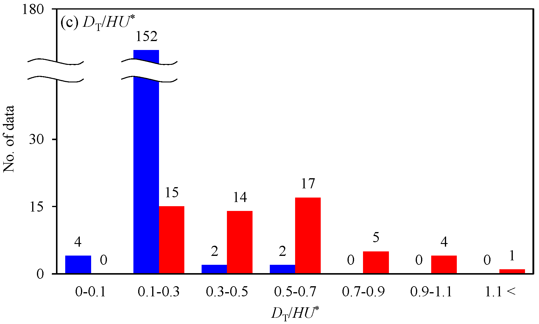
The statistical properties of the collected dataset were analyzed to establish regression models for D T . In total, 216 datasets were collected, consisting of 160 from laboratory channels and 56 from natural streams [1,6,8,9,11,46,47,48,49,50,51,52,53,54,55,56,57,58,59,60,61,62,63,64,65,66,67,68,69,70,71]. Laboratory experiments were predominantly conducted in straight channels, while 12 datasets [1,6] were obtained from meandering channels, exhibiting sinuosity ranging from 1.32 to 1.7. The corresponding Froude numbers for these experiments ranged from 0.032 to 0.972. Field experiments were conducted across streams in the USA, Canada, Europe, China, and South Korea; these were characterized by sinuosity ranging from 1.0 to 2.38, and the Froude number was in the range of 0.06–0.48. Fluorescent dye (specifically, Rhodamine B and Rhodamine WT) and neutrally buoyant solutions (such as nigrosine solution, gentian violet dye, carbon tetrachloride–benzine solution, etc.) were utilized for tracer tests in laboratory experiments; field experiments also employed fluorescent dye (Rhodamine B and Rhodamine WT). Table 1 presents the statistical properties for the laboratory channels and natural streams separately, focusing on W / H , U / U * and D T / H U * . Both data groups exhibited similar ranges and average values of U / U * . However, the average values of W / H and D T / H U * in natural streams were larger than those in the laboratory channels.
Figure 1 depicts histograms illustrating the distributions of the datasets. The statistical analysis revealed comparable distributions of U / U * in both the laboratory and the natural stream datasets. In contrast, W / H from the lab-scale experiments tended to accumulate in the range of W / H < 50 , resulting in relatively small values of D T / H U * compared to datasets from natural streams. Significantly, the abundance of lab-scale datasets, approximately three times larger than those from the natural streams, raises concerns about the narrowing applicability of empirical formulas for D T / H U * , developed from imbalanced datasets. To enhance the applicability of empirical formulas, it is imperative to augment the dataset by acquiring more experimental data of the natural stream scale.

2.2. Estimation of DT

In this study, D T was estimated using MLR, which is the traditional approach to obtain D T , and the nonlinear regression algorithms, which are SVR, XGBoost, and KNR; these are known to be efficient for the regression of nonlinear datasets [72,73,74]. Through dimensional analysis and theoretical derivations, dimensionless hydraulic parameters were derived to formulate empirical expressions for the dimensionless transverse dispersion coefficient ( D T / H U * ), as follows:
D T H U * = f W H ,   U U * ,   W R c ,   H R c ,   S n
where R c is the radius of curvature; S n is the channel sinuosity [10,18,71]. Table 2 presents the empirical formulas proposed using dimensionless hydraulic parameters suggested in previous studies. D T is primarily influenced by the vertical profiles of transverse velocity, as derived theoretically by Fischer et al. [14]. Therefore, hydraulic parameters such as bed friction ( U / U * ) and geometrical configurations ( W / H , H / R c , W / R c , and S n ), affecting vertical variations of transverse velocity, were incorporated into the formulas. The formulas, proposed by Jeon et al., Baek and Seo, and Yotsukura and Sayre [10,18,70], consider R c or S n to account for the effects of secondary currents. However, obtaining R c and S n is challenging due to the lack of information in the datasets. For instance, Jeon et al., and Baek and Seo [10,18] collected S n data from 16 and 18 field datasets, respectively. Aghababaei et al. [19] gathered 230 datasets, but only 49, including 29 field cases and 20 flume experiments, were available for S n . Consequently, establishing explainable relations between D T and S n from tracer test results, especially for natural streams with a large width-to-depth ratio, is challenging [12]. For these reasons, in this study, W / H and U / U * were considered as the input variables for estimating D T .
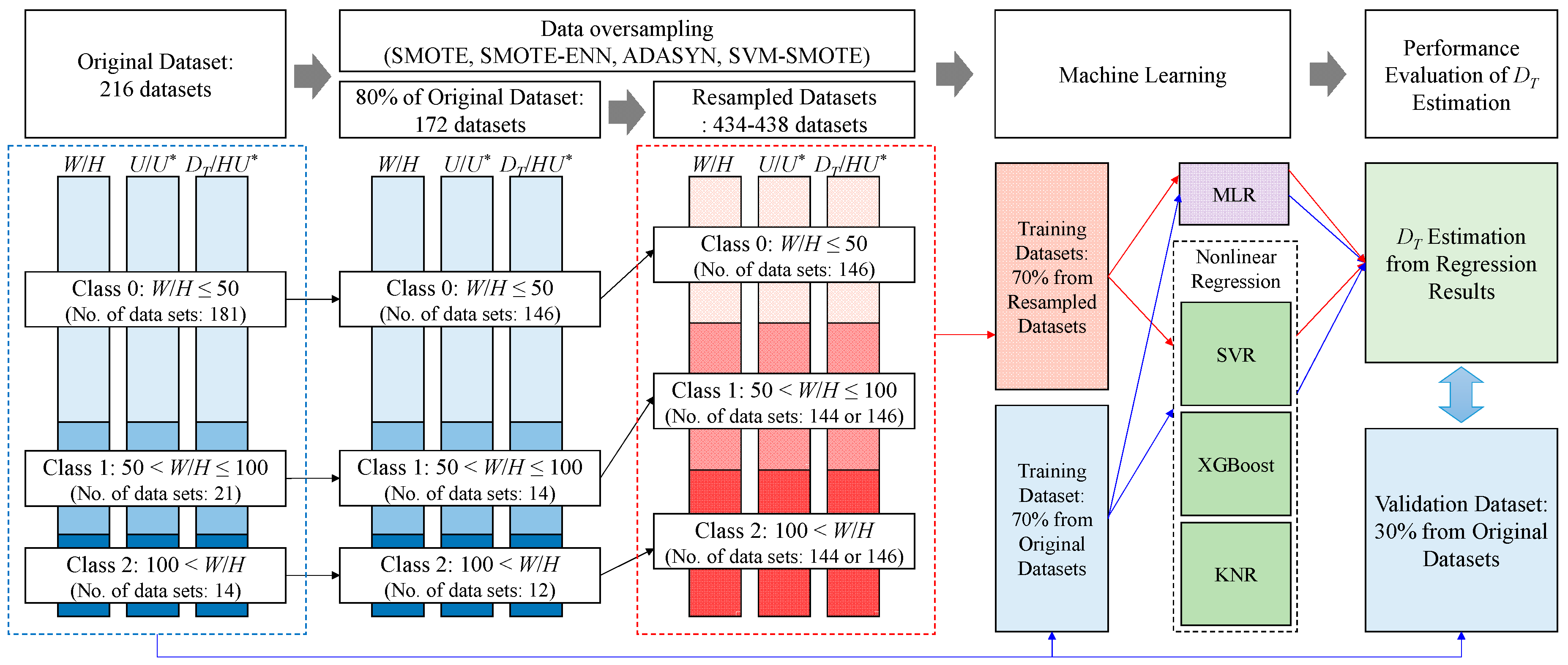
Figure 2 depicts the research procedure for obtaining D T from 216 datasets, as listed in Table 1. The datasets were classified across three ranges based on W / H : W / H < 50 (Class 0), 50 W / H < 100 (Class 1), and 100 W / H (Class 2), by the river scale, as proposed by Baek and Seo [71]. The original datasets consisted of 180 datasets in Class 0 (majority class), and 21 and 14 datasets in Class 1 and 2 (minority class), respectively. To generate new data, the training and validation datasets were split into 80% (172 datasets) and 20% (44 datasets), respectively, according to suggestions from previous studies [34,75,76]. Utilizing oversampling techniques, new datasets comprising W / H , U / U * , and D T / H U * were resampled from the training datasets classified as the minority class. After data oversampling, the dataset was divided into 70% training and 30% validation sets. D T was estimated using both the traditional MLR method and nonlinear regression methods, specifically SVR, XGBoost, and KNR. The Python Scikit-learn library (https://scikit-learn.org, accessed on 1 May 2024) [77] was utilized for conducting the aforementioned data regression in this study. From the MLR analysis, an empirical formula for D T was derived:
ln D T H U * = ln a + b ln W H + c ln U U *
where a, b, and c are empirical coefficients. The derived empirical formula and the three nonlinear regression models were evaluated by comparing them with 30% of test datasets extracted from the original datasets. The comparison results addressed the feasibility of using oversampling techniques to estimate D T in comparison to results obtained using the original datasets.

2.3. Data Oversampling

From the collected tracer test results, it is evident that there is an imbalance in the data concerning W / H , and this imbalance may lead to errors in the empirical formula for D T . In this study, we aim to address this data imbalance by employing oversampling techniques. The oversampling techniques chosen for this study are summarized in Table 3, which includes data resampling properties, advancements, and limitations of each oversampling technique.
SMOTE [34] generates synthetic data to increase the number of minority group instances, aiming to balance the overall dataset. SMOTE achieves this by resampling data from the k-nearest neighbors (KNN) within the minority group. The correct formula for generating synthetic data in SMOTE is as follows:
s i = x i + x n i x i · λ
where i is the sample number of a minority group, s i is the new synthetic data, x i is a sample from the minority group, x n i is a randomly selected data from the k-nearest neighbors within the minority group, and λ is a random number in the range of 0 and 1. The new data are created by interpolating among the minority group data, ensuring that the generated samples lie within the boundaries of the minority group.
The SMOTE-ENN algorithm [40] represents a hybrid approach, integrating SMOTE with ENN, an undersampling technique introduced by Wilson [79]. This method starts by generating synthetic data through SMOTE and subsequently employs ENN to eliminate instances identified as noisy and irrelevant. In ENN, synthetic data are classified as noisy if their class differs from the majority class among their k-nearest neighbors, with k set to 3. The incorporation of the ENN algorithm enhances the quality of the synthesized data group by effectively mitigating the introduction of misleading information or noise during the data synthesis process, as facilitated by SMOTE.
ADASYN [41] employs Equation (5) to generate new samples, and the number of resampled data ( N i ) is determined from the density distribution ( r ^ i ). N i is calculated as:
N i = r ^ i · n m j n m n λ
r ^ i = r i / i = 1 n m n r i = r i / i = 1 n m n Δ i / k
where n m j and n m n represent the number of majority and minority group data, respectively, r i = Δ i / k , k is the number of the nearest neighbors, and Δ i is the number of majority group data in the k-nearest neighbors of x i . From the calculations of N i and r ^ i , ADASYN algorithm synthesizes data, accounting for the difficulties in learning levels by assigning weights to minority group data.
SVM-SMOTE [78] is a variation of SMOTE, integrated with the support vector machine (SVM). The primary objective is to generate synthetic samples specifically in the feature space of the minority class. This approach aims to enhance the representation of the minority class through a combination of SVM principles and SMOTE. SVM-SMOTE generates new synthetic data as:
s i = s v i + s v i x i · λ
where s v i is the support vector by training SVM on x i . SVM-SMOTE prioritizes the augmentation of minority class instances near the decision boundaries, which are critical areas for boundary establishment. Furthermore, the generation of new instances strategically expands the minority class domain, particularly in regions with sparse majority class representation.
The four oversampling techniques were employed using the imbalanced-learn library from Python (https://www.jmlr.org/papers/v18/16-365.html, accessed on 1 May 2024) [80]. Accuracy, precision, recall, and F1 score were used to evaluate the classification performance of the oversampling techniques. These indices are calculated to validate the resampled data, as follows:
A c c u r a c y = T P + T N T P + T N + F P + F N
P r e c i s i o n = T P T P + F P
R e c a l l = T P T P + T N + F P + F N
F 1 = 2 × P r e c i s i o n × R e c a l l P r e c i s i o n × R e c a l l
where TP (true positive) represents the number of samples accurately predicted as positive, TN (true negative) indicates the number of samples accurately predicted as negative, FP (false positive) is the count of samples falsely predicted as positive, and FN (false negative) denotes the number of samples falsely predicted as negative. In addition, the statistical similarity of the oversampled data to the original data was assessed using the Kolmogorov–Smirnov test (KS test) [81], which compared the cumulative distribution functions of the two datasets.

2.4. Machine Learning Regression Methods

2.4.1. Support Vector Machine Regression (SVR) Model

SVR is an extension of the support vector machine (SVM) algorithm, which is primarily used for data classification. SVM aims to determine a hyperplane that maximizes the margin around the given dataset, ensuring that each data point lies within the margin boundary [82]. SVR addresses regression problems by mapping nonlinear data to a higher-dimensional space using kernel functions, transforming low-dimensional nonlinear regression problems into high-dimensional linear regression problems [72]. Consequently, SVR solves the regression problem by maximizing the margin from the given dataset x i ,   y i through the following optimization problem:
minimize   1 2 w 2 + C i = 1 l ξ i + ξ i * subject   to   y i w T x i + b ε + ξ i * w T x i + b y i ε + ξ i ξ i ,   ξ i * 0 ,   i = 1 , . . l  
where w is the weighting vector, C is a positive constant, ξ i   and   ξ i * are slack variables used to estimate the deviation between actual data and a predicted data, b is a bias term, and ε is the margin. The kernel function employed for this study is the radial basis function (RBF), as follows:
k x i , x j = exp ( γ x i x j 2 )
where x i   and   x j are data points and γ is a parameter for the RBF kernel function.

2.4.2. eXtream Gradient Boosting Regression (XGBoost) Model

XGBoost is a machine learning regression model that applies the gradient boosting algorithm, known for its advantages in parallel processing and optimization in solving both classification and regression problems [83]. XGBoost is an ensemble technique that combines multiple decision trees to create an ensemble model for nonlinear regression. A decision tree is a method that classifies data by stacking multiple binary nodes with various conditions to predict the final value. For instance, in a scenario with three decision tree models, M 1 , M 2 , M 3 , boosting adjusts the weights of poorly predicted samples x i in M 1 to train M 2 , and similarly adjusts weights for poorly predicted samples x i in M 2 to train M 3 , and so on. The final prediction is obtained by combining predictions from each model with their respective weights, W n , as shown in Equation (14).
y i = i = 1 K W i M i x i + ε j x j
where K is the number of decision trees. This boosting technique, implemented in XGBoost, differs from traditional gradient boosting as it incorporates weight assignments for regularization, which helps reduce overfitting. Furthermore, XGBoost allows users to define optimization goals and evaluation criteria, and it includes built-in routines to handle missing values, enabling various learning experiments [83].

2.4.3. k–Nearest Neighbors Regression (KNR) Model

KNR algorithm is a method used in machine learning regression models to predict results for new inputs by utilizing information from the k-nearest data points [84]. KNR offers a flexible approach by considering the local structure of the data. The algorithm does not assume any specific functional form for the relationship between the predictors and the response variable, making it suitable for capturing complex nonlinear patterns in the data. When estimating the desired value, the algorithm calculates the distance from each of the k-nearest data points in the given dataset. For this purpose, Euclidean distance is employed to measure distances between the training data points. The Euclidean distance ( d ) between two points, X x 1 ,   x 1 ,   ,   x n and Y y 1 ,   y 1 ,   ,   y n , is defined by the following equation:
d = x 1 y 1 2 + x 2 y 2 2 + + x n y n 2
In a regression model that outputs numerical values, the output is the mean value of the k-nearest neighbors, where weights inversely proportional to the distances of the neighboring points are applied and averaged. Given the k-nearest neighbor, when the input x is provided, the output, y, is computed using both the mean value, Equation (16), and the weighted mean value, Equation (17).
y = 1 k i = 1 k y i
y = i = 1 k w i y i i = 1 k w i w i = 1 d X ,   X i
In this study, to determine the nearest neighbor count K for the data samples, the value of K that minimizes the root mean square error (RMSE) was selected from the range of 1 to 20.

3. Results

3.1. Oversampling Results and Performance Evaluations

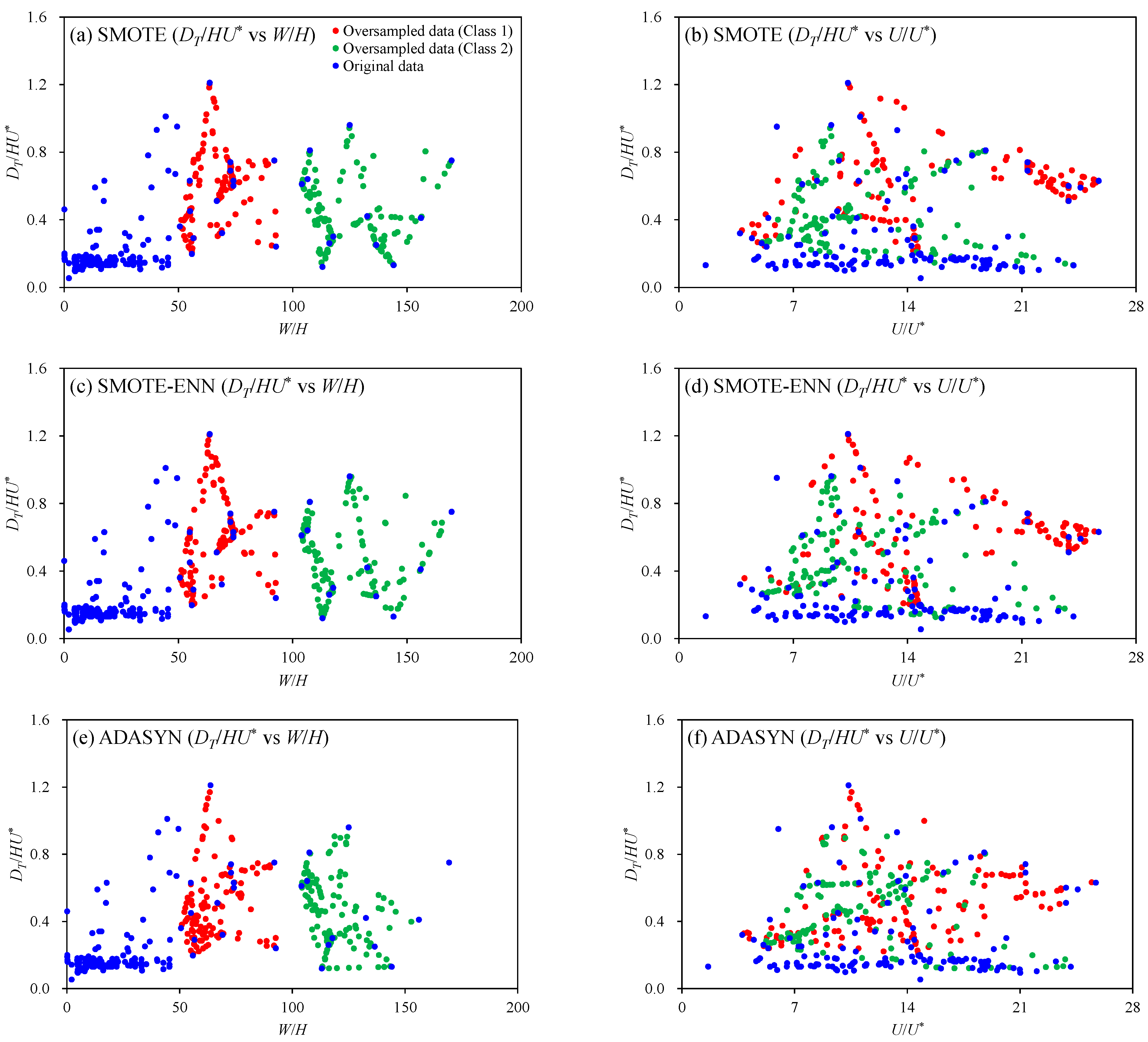
The transverse dispersion coefficients and accompanying hydraulic data were resampled using four oversampling techniques, SMOTE, SMOTE-ENN, ADASYN, and SVM-SMOTE. The data of W / H , U / U * , and D T / H U * included in minority classes (classes 1 and 2 depicted in Figure 2) were resampled and plotted with original datasets in Figure 3. The number of resampled data increased from 216 to 438 using SMOTE and SVM-SMOTE and rose to 436 and 434 using SMOTE-ENN and ADASYN, respectively. Since oversampling is based on the classification according to the range of W / H , the classes of the resampled data are clearly distinguished in Figure 3a. However, the classes among the resampled data based on U / U * are not as clearly distinguished (Figure 3b), and therefore are represented based on the classification according to W / H . SMOTE-ENN, being rooted in SMOTE, exhibited a similar distribution in the resampled data and generated data points between the original data using the KNN technique. In contrast, ADASYN adapts its sampling density according to the local distribution of minority class samples, resulting in increased sampling around the borderline instances, as depicted in the relatively higher density near the boundary of the Classes 1 and 2. SVM-SMOTE, leveraging the SVM algorithm, generates synthetic samples focusing on regions that are difficult to classify, thereby reinforcing the characteristics of the minority class by creating data points centered on specific instances.
The resampled datasets were evaluated based on two criteria: whether the newly generated dataset was accurately classified according to the original dataset’s class distribution, and whether it exhibited statistically similar characteristics to the original dataset. For the assessments, the calculation results using the classification performance indicators (Equations (8)–(11)) and p-values from the KS test were included in Table 4 for comparing the performance of the resampled datasets. Both the classification performance indicators and the KS test results indicate that all tested oversampling techniques provide acceptable results. Specifically, the results obtained by SMOTE outperformed the other oversampling techniques, followed by SMOTE-ENN, SVM-SMOTE, and ADASYN. However, in line with the purpose of this study, it is required to test whether the resampled data are applicable to estimate D T / H U * beyond the statistical reproducibility of the datasets.

3.2. DT Predictions Using MLR

From both the original and resampled datasets, empirical formulas were derived using the conventional method, multiple linear regression (MLR). The training dataset for obtaining empirical coefficients of Equation (3) using MLR was 70% of each oversampled dataset. The derived empirical coefficients are listed in Table 5. The results obtained using the original dataset indicate a larger value of b compared to c, suggesting that the effects of W / H are more dominant than those of U / U * in determining the transverse dispersion coefficient. Except for the results in SMOTE, larger weighting in W / H appeared even though there are differences in degree. The results by SMOTE suggested more weighting in U / U * .
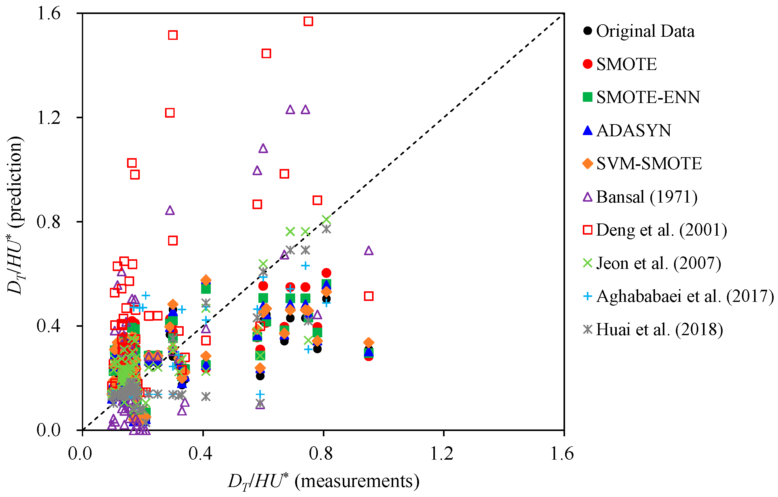
D T / H U * was estimated using derived empirical formulas and compared with measurements. This comparison was conducted using a validation dataset comprising 30% of the original dataset. Figure 4 shows the comparison results of D T / H U * , plotted alongside computation results using empirical formulas presented in Table 2. The accuracy of the estimated results was evaluated using the mean absolute percentage error (MAPE), as follows:
MAPE = i = 1 n O i P i O i
where O i is the measurements, P i is the estimated value, and n is the number of validation datasets. The calculation results of MAPE are presented in Table 6. MAPE was computed for both the entire validation set and for separated sets based on the range of W / H . For the entire validation set, MAPE calculation results from the oversampled dataset-derived empirical formulas demonstrated lower accuracy compared to the results using the original dataset. This lower accuracy in the oversampling results is attributed to the majority class dataset ( W / H 50 ), which resulted in large errors. Conversely, for the minority class dataset ( W / H > 50 ), which incorporates the resampled data, MAPE calculations resulted in higher accuracy compared to the results obtained using the original dataset across all oversampling techniques. These results indicate that data oversampling improves the estimation accuracy, especially for the minority class ( W / H > 50 ). However, the empirical formulas were strongly influenced by the resampled data, particularly as the number of resampled data points in the majority class ( W / H 50 ) was approximately doubled, resulting in decreased performance in the estimation of D T / H U * for the majority class.
The MAPE calculation results from the formulas listed in Table 2 reveal that the results by Huai et al. [30] exhibited the highest accuracy, and among the formulas derived through MLR, the results by Jeon et al. [10] showed the highest accuracy. Despite using data from natural streams, Jeon et al. [10] achieved higher accuracy than the results presented in this study by utilizing three variables ( W / H , U / U * , and S n ) for the entire W / H ranges. Consequently, even with data imbalance alleviated through oversampling, there may be limitations in improving accuracy when using MLR to obtain estimates of D T / H U * . These results suggest that, in developing empirical formulas using MLR, the application of more variables may be more advantageous than increasing the number of data points. However, since empirical formulas derived from MLR are based on the linearity between independent and dependent variables, there are limitations to improving accuracy. Therefore, empirical formulas developed through GP suggested by Agababaei et al., and Huai et al. [19,30] outperformed compared to those obtained by Jeon et al. [10] using MLR. However, determining whether the results of Agababaei et al., and Huai et al. [19,30] were due to improved accuracy through nonlinear regression analysis or an increase in the number of data is challenging, as they utilized more data and three or more variables ( W / H , U / U * , S n , and Fr) for empirical formula derivation compared to the study by Jeon et al. [10]. This suggests that there is a need for applying nonlinear regression analysis for transverse dispersion coefficient estimation and implies the necessity of verifying whether applying nonlinear regression analysis can overcome the limitations of using a limited number of regression variables.

3.3. DT Predictions Using Nonlinear Regression Methods

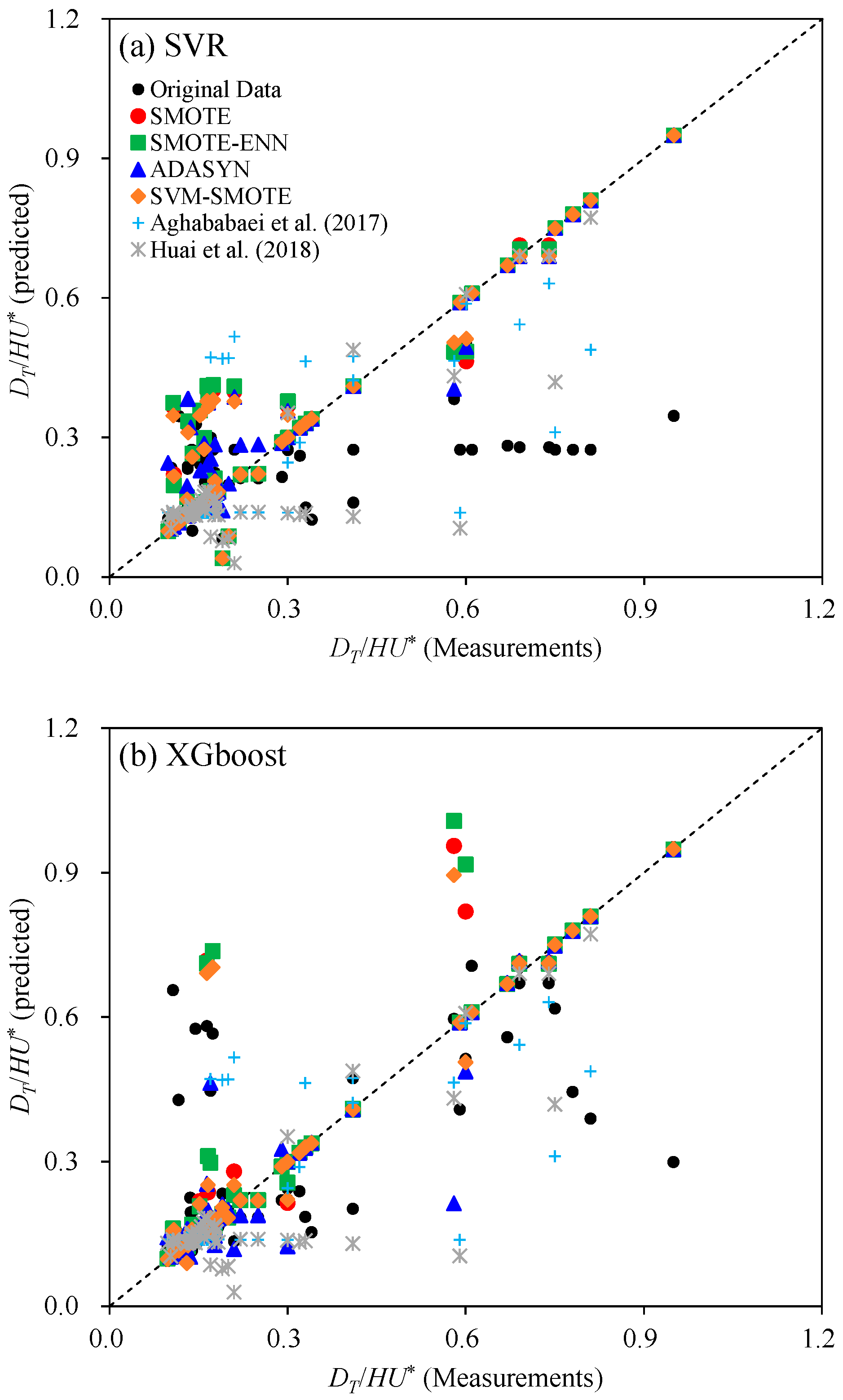
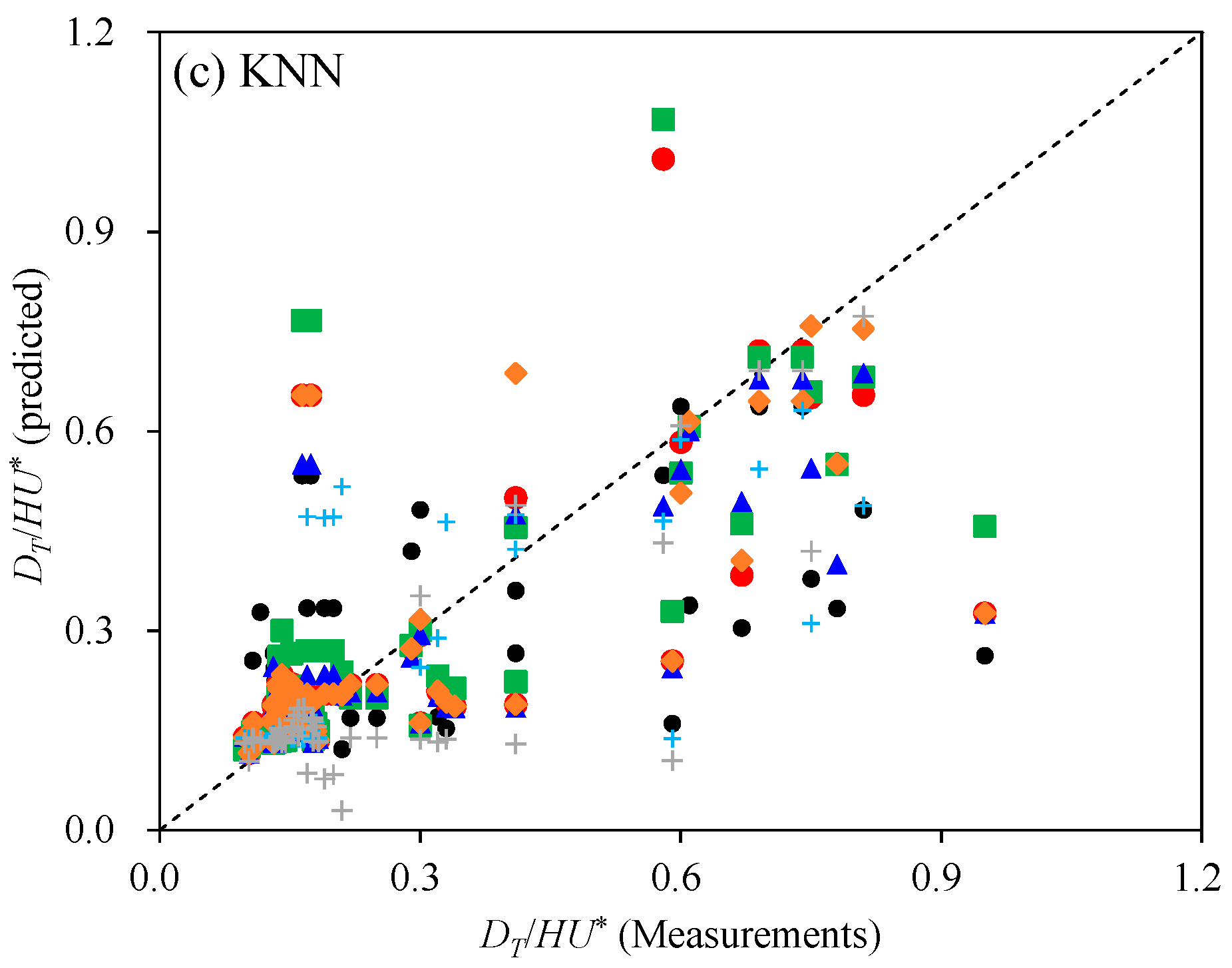
D T / H U * was estimated using nonlinear regression methods, including SVR, XGBoost, and KNR, applied to both the original and resampled datasets. During the data learning phase, 70% of each dataset was utilized to train the nonlinear regression models. Subsequently, the trained regression models were applied to estimate D T / H U * for the validation dataset, which corresponded to the dataset depicted in Figure 4. The estimation results is presented in Figure 5, where the results by Aghababei et al., and Huai et al. [19,30] are also plotted for comparison. The results obtained using nonlinear regression models, as depicted in Figure 5, exhibit significant improvement compared to those in Figure 5, with a larger proportion of estimations closely aligned along the diagonal line. Computation results of MAPE, provided in Table 7, underscore this enhancement. Notably, the original data yielded a MAPE of 43.6%, representing an improvement over MLR (MAPE = 53.4%). Particularly noticeable improvements were observed in the results derived from the resampled datasets, with averaged MAPE ranging from 20.9% to 25.5% across different oversampling techniques. These values significantly outperformed those shown in Table 4 (MAPE = 57.2% to 67.3%).
The results obtained using the resampled data demonstrate comparable accuracy to those obtained by Aghababaei et al., and Huai et al. [19,30]. An encouraging aspect is that the results presented in this study improved accuracy using only two variables ( W / H and U / U * ), while Aghababaei et al., and Huai et al. [19,30] utilized four and three variables, respectively. For the resampled dataset range ( W / H > 50 ), the combination of SVM-SMOTE and SVR yielded the most accurate results. However, it is worth noting that the results of SVM-SMOTE were deemed to be overfitted for the data belonging to W / H > 50 , leading to a decrease in accuracy in the range of W / H 50 . Thus, the best combination of an oversampling technique and a nonlinear regression model was found to be ADASYN and XGboost. Specifically, the datasets resampled by ADASYN provided the best results in every case using the three nonlinear regression methods. These results suggest that the combination of ADASYN and the nonlinear regression methods offers comparatively improved results, especially in the non-oversampled data range ( W / H 50 ).

4. Discussion

4.1. DT Estimation Performance Using MLR through Data Augmentation

The efficacy of empirical formulas in estimating D T relies on both accuracy and expansibility. The acquisition of data plays a crucial role in enhancing the performance of D T estimation through empirical formulas derived by MLR. However, the limited availability of datasets for W / H > 50 poses constraints on improving the performance of empirical formulas. Among the 216 datasets collected in this study, 181 correspond to W / H 50 , while 35 correspond to W / H > 50 . Therefore, there is a risk of deriving overfitted equations for W / H > 50 datasets when estimating D T using datasets biased towards W / H 50 . To improve the accuracy of the estimation, it is necessary to either increase the number of variables or acquire new datasets including W / H > 50 . However, there are limitations due to the increase in the complexity of the estimation and the need to obtain results from field tracer tests.
To address the limitation of insufficient measured data, this study employed oversampling techniques to generate new datasets within the W / H > 50 range, ensuring that the generated data reflects the statistical properties of the original data, as validated by the KS test (Table 4). The empirical formulas derived with W / H and U / U * from the oversampled data demonstrated improved accuracy within the W / H > 50 range compared to the pre-oversampling results (Table 5). Nevertheless, when considering the accuracy for the W / H 50 range, the formula utilizing the original dataset exhibited higher accuracy than those using oversampled data. These findings underscore the idea that data point increase is insufficient for enhancing the performance of an empirical formula derived through MLR. Therefore, as proposed by Baek and Seo [71], it is imperative to apply distinct empirical formulas based on W / H . Alternatively, increasing the complexity of empirical formulas by incorporating additional variables or employing nonlinear regression methods would offer a viable solution.
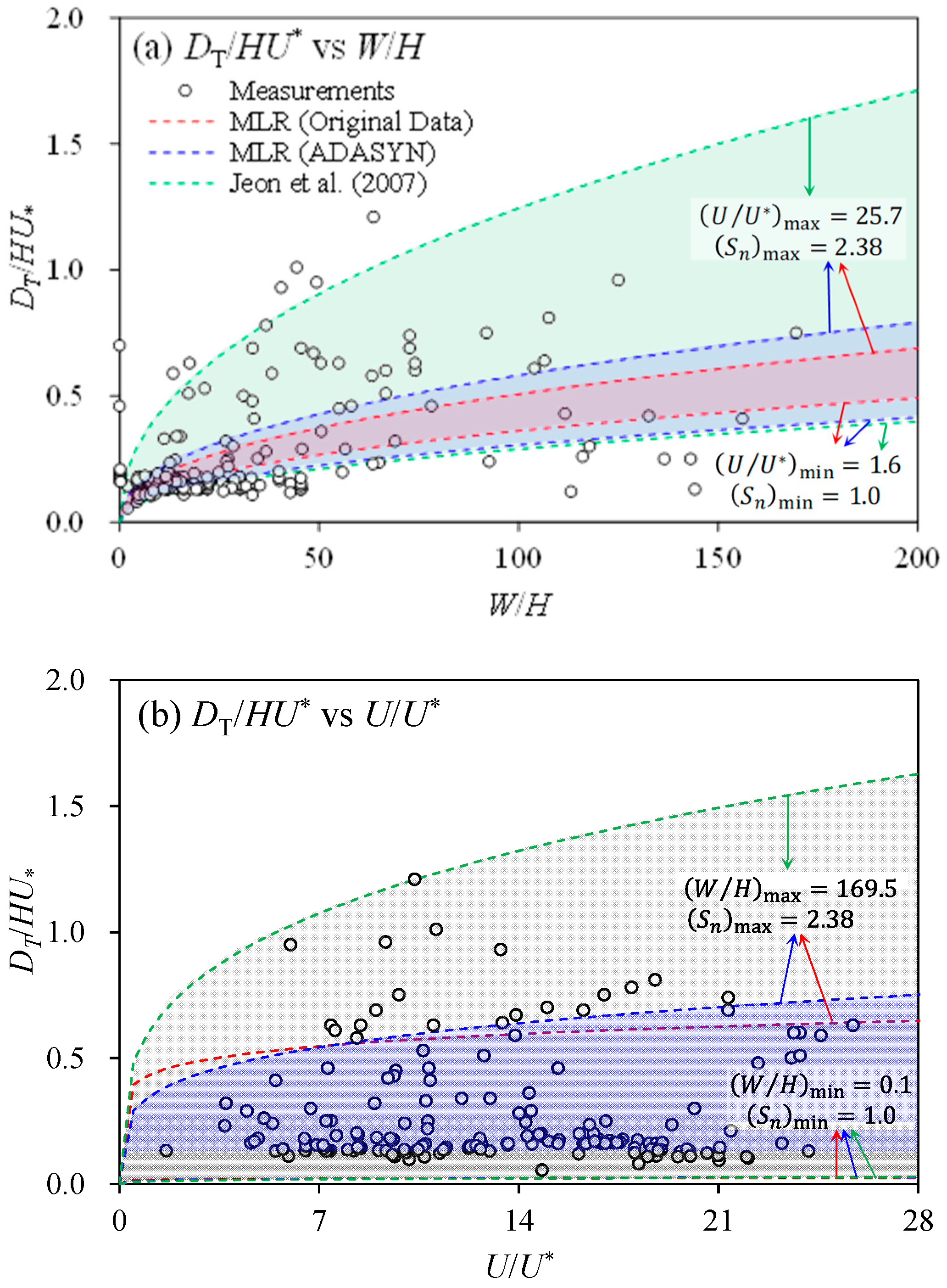
The range of reproducible D T / H U * through empirical formulas including two variables ( W / H and U / U * ) demonstrates the extendibility of the developed formula. Figure 6 shows the range of D T / H U * derived from empirical formulas developed using original and oversampled data by ADASYN. To depict the possible range of D T / H U * concerning the variation in W / H , the upper and lower boundaries were determined by applying the maximum and minimum values of U / U * from the original dataset (Figure 6a). Similarly, the calculable range concerning the variation in U / U * was determined by applying the maximum and minimum values of W / H (Figure 6b). These results indicate that the range of D T / H U * widens when utilizing empirical formulas derived from an oversampled dataset. This suggests that empirical formulas derived from resampled datasets may possess higher applicability than those utilizing only original data. However, compared to the reproducible range proposed by Jeon et al. [10] using three variables ( W / H , U / U * , and S n ), these findings reveal a considerably limited reproducible range. Additionally, as indicated in Table 6, despite using only 32 field datasets, the results by Jeon et al. [10] exhibited the highest accuracy among those derived using MLR. Hence, these results indicate that adding variables that account for secondary currents’ effects on transverse dispersion is more effective in improving D T estimation performance than increasing the number of datasets. Consequently, data oversampling may offer limited enhancements to D T estimation performance when employing MLR.

4.2. Comparisons of DT Estimation Results Using MLR and Nonlinear Regression Methods

In this study, original tracer test datasets (216 datasets) and resampled datasets (434–438 datasets) were used for estimating D T (see Figure 2). Of these datasets, 70% were classified as training datasets to derive empirical formulas for D T estimation using MLR and three nonlinear regression models: SVR, XGBoost, and KNR. The accuracy of the D T estimations obtained through each method was compared using MAPE based on a range of W / H values, using a validation dataset comprising 30% of the data (Table 6 and Table 7). Results derived from MLR using two variables ( W / H and U / U * ) from the original dataset (Table 5) showed errors of 53.5% for W / H 50 and 37.1% for W / H > 50 (Table 6). These results exhibited similar performance to those derived using formulas developed by Jeon et al. [10] based on three parameters, W / H , U / U * , and S n , with errors of 55.5% for W / H 50 and 23.9% for W / H > 50 . Jeon et al. [10] developed D T estimation formulas using 32 tracer test datasets from natural streams, demonstrating that increasing the number of datasets, instead of incorporating S n into the estimation formulas, could enhance the performance of MLR-based estimations. However, increasing the number of datasets through oversampling had limitations in improving MLR-based estimations, and resulted in larger errors than results derived solely from original data. These limitations using MLR were reduced by employing machine-learning-based nonlinear regression methods, as demonstrated in the studies by Aghababaei et al., and and Huai et al. [19,30], through the utilization of additional variables (Table 6).
Adding variables for D T estimation may increase the complexity of the estimation formulas and may have limited applicability. Therefore, instead of adding variables, we investigated the performance-improvement effect through D T estimation using nonlinear regression methods (SVR, XGBoost, and KNR) (Table 7). The results showed that estimations using W / H and U / U * from the original dataset had average errors of 46.0% and 30.4% for W / H 50 and W / H > 50 , respectively, indicating improved performance compared to MLR-based estimations. The performance-improvement effect through nonlinear regression methods was further enhanced when using resampled datasets, particularly when estimating D T using XGBoost from datasets resampled using ADASYN; this showed errors of 11.0% and 10.7% for W / H 50 and W / H > 50 , respectively, outperforming MLR-based D T estimations. These results demonstrated improved performance compared to the utilization of estimation formulas by Huai et al. [30] based on three variables, W / H , U / U * , and S n , which showed errors of 15.0% and 14.9% for W / H 50 and W / H > 50 , respectively. In conclusion, considering these results, machine-learning-based nonlinear regression methods were found to be more effective than MLR for D T estimation; additionally, using data oversampling to alleviate dataset imbalance yielded superior performance in D T estimation compared to the effects of increasing variables.

4.3. The Feasibility of Two Variables for DT Estimation

The results presented in Table 7 demonstrate that the combination of data oversampling and a nonlinear regression method improves the accuracy of D T estimation using only W / H and U / U * . The previous discussion in Section 4.1 discussed the potential of incorporating S n to extend the predictability range of D T . While incorporating S n could potentially improve the accuracy of estimations, its availability to consider the effects of secondary currents on transverse dispersion is considerably restricted for the present datasets. Although W / H and U / U * were commonly available in all datasets collected in this study, the utilization of hydraulic parameters such as R c or S n to reflect flow structures such as secondary currents are highly limited. Furthermore, Gond et al. [12] presented that even in rivers with S n close to 1, D T can be significantly increased due to longitudinal flow nonuniformity; however, the lack of sufficient data hinders the utilization of this information in D T estimation. Hence, until sufficient research data are secured to enhance the regression accuracy of D T , the application of methodologies to improve D T estimation accuracy using common variables such as W / H and U / U * , obtainable across previously published papers, is required.
As demonstrated in Table 7, the combination of the ADASYN–XGBoost method improved D T estimation accuracy using only W / H and U / U * . To assess the improvement effect of including S n in MLR results, an empirical formula including S n , similar to that proposed by Jeon et al. [10], was derived from the datasets collected in this study, yielding Equation (19):
D T H U * = 0.051 U U * 0.17 W H 0.32 S n 1.1
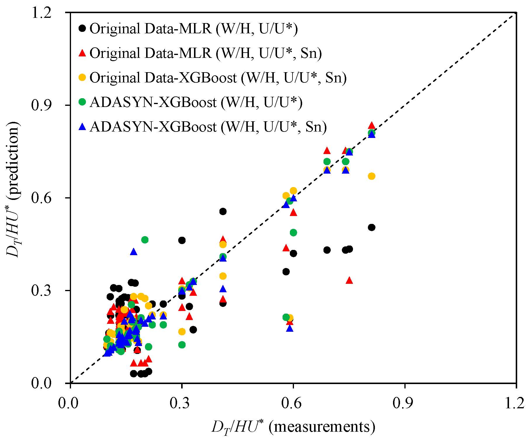
Additionally, utilizing the XGBoost regression combined with the oversampling technique of ADASYN, data resampling was performed on 195 datasets where S n could be applied out of the 216 original datasets. S n for the straight channel was set to 1 (152 datasets). Through the resampling, the total dataset increased to 406, with the average S n value increasing from 1.09 to 1.22 and the median increasing from 1.0 to 1.12. D T was estimated through XGBoost, using the resampled data including S n . Figure 7 compares the D T estimation results obtained through MLR and XGBoost, excluding field-scale data without S n information among validation datasets shown in Figure 5. Table 8 presents the MAPE calculation results for D T estimation and the accuracy improvement effect of each D T estimation result compared to the results from MLR with two variables ( W / H and U / U * ). Both MLR and XGBoost yielded higher accuracy when incorporating three variables ( W / H , U / U * , and S n ) compared to utilizing only two variables ( W / H and U / U * ) for both the original and oversampled datasets, respectively. Moreover, the XGBoost regression results using oversampled data consisting of only two variables demonstrated higher accuracy than the XGBoost regression results from the original dataset including S n . Thus, it can be concluded that data oversampling resolves the issue of reduced D T estimation performance due to variable scarcity, and significant improvements in accuracy comparable to those from increasing variables can be achieved using only W / H and U / U * .

5. Conclusions

In this study, we addressed the issue of reduced D T estimation performance due to the data imbalance, in which the datasets are accumulated in W / H 50 from the data resampling employing four oversampling techniques, SMOTE, SMOTE-ENN, ADASYN, and SVM-SMOTE. From the resampled datasets, D T was estimated using both MLR and three machine learning regression algorithms, SVR, XGBoost, and KNR. The estimated D T was compared to the empirical formulas proposed by previous research to evaluate performance of D T estimation by reducing the data imbalance. The results revealed that there was no significant improvement in accuracy with MLR using the oversampled datasets. However, when employing nonlinear regression methods, the effectiveness of accuracy improvement due to data oversampling increased substantially. Notably, when estimating D T using only two variables, W / H and U / U * , through the ADASYN–XGBoost method, a higher improvement in performance was observed compared to XGBoost regression results from the original dataset, including S n . These findings suggest that data oversampling is more effective than increasing the number of variables for employing nonlinear regression. While data oversampling cannot replace field data acquisition, it provides benefits such as improving the accuracy of imbalanced data and enhancing D T estimation accuracy using minimal variables and restricted tracer test data.

Author Contributions

Conceptualization, S.L. and I.P.; methodology, S.L. and I.P.; software, S.L. and I.P.; validation, S.L. and I.P.; formal analysis, S.L.; investigation, S.L.; resources, S.L. and I.P.; data curation, S.L.; writing—original draft preparation, S.L. and I.P.; writing—review and editing, I.P.; visualization, S.L. and I.P.; supervision, I.P.; project administration, I.P.; funding acquisition, I.P. All authors have read and agreed to the published version of the manuscript.

Funding

This study was financially supported by Seoul National University of Science and Technology.

Data Availability Statement

The data presented in this study will be shared by the authors if requested.

Acknowledgments

This study was conducted by the financial support by Seoul National University of Science and Technology.

Conflicts of Interest

The authors declare no conflicts of interest.

References

  1. Shin, J.; Seo, I.W.; Baek, D. Longitudinal and transverse dispersion coefficients of 2D contaminant transport model for mixing analysis in open channels. J. Hydrol. 2020, 583, 124302. [Google Scholar] [CrossRef]
  2. Piasecki, M.; Katopodes, N.D. Identification of stream dispersion coefficients by adjoint sensitivity method. J. Hydraul. Eng. 1999, 125, 714–724. [Google Scholar] [CrossRef]
  3. King, I.; Letter, J.V.; Donnel, B.P. RMA4 Users Guide 4.5x; US Army, Engineer Research and Development Center, WES, CHL: Vicksburg, MI, USA, 2008. [Google Scholar]
  4. Lee, M.E.; Seo, I.W. Analysis of pollutant transport in the Han River with tidal current using a 2D finite element model. J. Hydro-environ. Res. 2007, 1, 30–42. [Google Scholar] [CrossRef]
  5. Park, I.; Seo, I.W.; Shin, J.; Song, C.G. Experimental and numerical investigations of spatially-varying dispersion tensors based on vertical velocity profile and depth-averaged flow field. Adv. Water Res. 2020, 142, 103606. [Google Scholar] [CrossRef]
  6. Baek, K.O.; Seo, I.W.; Jeong, S.J. Evaluation of dispersion coefficients in meandering channels from transient tracer tests. J. Hydraul. Eng. 2006, 132, 1003–1119. [Google Scholar] [CrossRef]
  7. Seo, I.W.; Lee, M.E.; Baek, K.O. 2D modeling of heterogeneous dispersion in meandering channels. J. Hydraul. Res. 2008, 44, 350–362. [Google Scholar] [CrossRef]
  8. Tabatabaei, S.H.; Heidarpour, M.; Ghasemi, M.; Hoseinipour, E.Z. Transverse mixing coefficient on dunes with vegetation on a channel wall. In Proceedings of the World Environmental and Water Resources Congress 2013: Showcasing the Future, Cincinnati, OH, USA, 19–23 May 2013; pp. 1903–1911. [Google Scholar]
  9. Beltaos, S. Transverse mixing tests in natural streams. J. Hydraul. Div. 1980, 106, 1607–1625. [Google Scholar] [CrossRef]
  10. Jeon, T.M.; Baek, K.O.; Seo, I.W. Development of an empirical equation for the transverse dispersion coefficient in natural streams. Environ. Fluid Mech. 2007, 7, 317–329. [Google Scholar] [CrossRef]
  11. Seo, I.W.; Choi, H.J.; Kim, Y.D.; Han, E.J. Analysis of two-dimensional mixing in natural streams based on transient tracer tests. J. Hydraul. Eng. 2016, 142, 04016020. [Google Scholar] [CrossRef]
  12. Gond, L.; Mignot, E.; Le Coz, J.; Kateb, L. Transverse mixing in rivers with longitudinally varied morphology. Water Resour. Res. 2020, 57, e2020WR029478. [Google Scholar] [CrossRef]
  13. Jung, S.H.; Seo, I.W.; Kim, Y.D.; Park, I. Feasibility of velocity-based method for transverse mixing coefficients in river mixing analysis. J. Hydraul. Eng. 2019, 145, 04019040. [Google Scholar] [CrossRef]
  14. Fischer, H.B.; List, J.E.; Koh, R.C.Y.; Imberger, J.; Brooks, N.H. Mixing in Inland and Coastal Waters, 2nd ed.; Academic Press: San Diego, CA, USA, 1979; pp. 80–147. [Google Scholar]
  15. Rutherford, J.C. River Mixing; John Wiley and Sons: London, UK, 1994; pp. 62–63. [Google Scholar]
  16. Gharbi, S.; Verrette, J.L. Relation between longitudinal and transversal mixing coefficients in natural streams. J. Hydraul. Res. 1998, 36, 43–54. [Google Scholar] [CrossRef]
  17. Deng, Z.Q.; Singh, V.P.; Bengtsson, L. Longitudinal dispersion coefficient in straight rivers. J. Hydraul. Eng. 2001, 127, 919–927. [Google Scholar] [CrossRef]
  18. Baek, K.O.; Seo, I.W. Empirical equation for transverse dispersion coefficient based on theoretical background in river bends. Environ. Fluid Mech. 2013, 13, 465–477. [Google Scholar] [CrossRef]
  19. Aghababaei, M.; Etemad-Shahidi, A.; Jabbari, E.; Taghipour, M. Estimation of transverse mixing coefficient in straight and meandering streams. Water Resour. Manag. 2017, 31, 3809–3827. [Google Scholar] [CrossRef]
  20. Baek, K.O.; Lee, D.Y. Development of simple formula for transverse dispersion coefficient in meandering rivers. Water 2023, 15, 3120. [Google Scholar] [CrossRef]
  21. Tao, H.; Al-Khafaji, Z.S.; Qi, C.; Yassen, Z.M. Artificial intelligence models for suspended river sediment prediction: State-of-the art, modeling framework appraisal, and proposed future research directions. Eng. Appl. Comput. Fluid Mech. 2021, 15, 1585–1612. [Google Scholar] [CrossRef]
  22. Tayfur, G.; Singh, V.P. Predicting longitudinal dispersion coefficient in natural streams by artificial neural network. J. Hydraul. Eng. 2005, 131, 991–1000. [Google Scholar] [CrossRef]
  23. Noori, R.; Karbassi, A.; Farokhnia, A.; Dehghani, M. Predicting the longitudinal dispersion coefficient using support vector machine and adaptive neuro-fuzzy inference system techniques. Environ. Eng. Sci. 2009, 26, 1503–1510. [Google Scholar] [CrossRef]
  24. Sattar, A.M.A.; Gharabaghi, B. Gene expression models for prediction of longitudinal dispersion coefficient in streams. J. Hydrol. 2015, 524, 587–596. [Google Scholar] [CrossRef]
  25. Seifi, A.; Riahi-Madvar, H. Improving one-dimensional pollution dispersion modeling in rivers using ANFIS and ANN-based GA optimized models. Environ. Sci. Pollut. Res. 2019, 26, 867–885. [Google Scholar] [CrossRef]
  26. Azar, N.A.; Milan, S.G.; Kayhomayoon, Z. The prediction of longitudinal dispersion coefficient in natural streams using LS-SVM and ANFIS optimized by Harris hawk optimization algorithm. J. Contam. Hydrol. 2021, 240, 103781. [Google Scholar] [CrossRef] [PubMed]
  27. Ghiasi, B.; Noori, R.; Sheikhian, H.; Zeynolabedin, A.; Sun, Y.; Jun, C.; Hamouda, M.; Bateni, S.M.; Abolfathi, S. Uncertainty quantification of granular computing-neural network model for prediction of pollutant longitudinal dispersion coefficient in aquatic streams. Sci. Rep. 2022, 12, 4610. [Google Scholar] [CrossRef] [PubMed]
  28. Ohadi, S.; Monfared, S.A.H.; Moghaddam, M.A.; Givehchi, M. Feasibility of a novel predictive model based on multilayer perceptron optimized with Harris hawk optimization for estimating of the longitudinal dispersion coefficient in rivers. Neural Comp. Appl. 2023, 35, 7081–7105. [Google Scholar] [CrossRef]
  29. Azamathulla, H.M.; Ahmad, Z. Gene-expression programming for transverse mixing coefficient. J. Hydrol. 2012, 434–435, 142–148. [Google Scholar] [CrossRef]
  30. Huai, W.; Shi, H.; Yang, Z.; Zeng, Y. Estimating the transverse mixing coefficient in laboratory flumes and natural rivers. Water Air Soil Pollut. 2018, 229, 252. [Google Scholar] [CrossRef]
  31. Zahiri, J.; Nezaratian, H. Estimation of transverse mixing coefficient in streams using M5, MARS, GA, and PSO approaches. Environ. Sci. Pollut. Res. 2020, 27, 14553–14566. [Google Scholar] [CrossRef] [PubMed]
  32. Nezaratian, H.; Zahiri, J.; Peykani, M.F.; Haghiabi, A.; Parsaie, A. A genetic algorithm-based support vector machine to estimate the transverse mixing coefficient in streams. Water Qual. Res. J. 2021, 56, 128. [Google Scholar] [CrossRef]
  33. Najafzadeh, M.; Noori, R.; Afroozi, D.; Ghiasi, B.; Hosseini-Moghari, S.M.; Mirchi, A.; Haghighi, A.T.; Kløve, B. A comprehensive uncertainty analysis of model-estimated longitudinal and lateral dispersion coefficients in open channels. J. Hydrol. 2021, 603, 126850. [Google Scholar] [CrossRef]
  34. Chawla, N.V.; Bowyer, K.W.; Hall, L.O.; Kegelmeyer, W.P. SMOTE: Synthetic Minority Over-sampling Technique. J. Artif. Intell. Res. 2002, 16, 321–357. [Google Scholar] [CrossRef]
  35. Huang, R.; Ma, C.; Ma, J.; Huangfu, X.; He, Q. Machine learning in natural and engineered water systems. Water Res. 2021, 205, 117666. [Google Scholar] [CrossRef]
  36. Xu, T.; Coco, G.; Neale, M. A predictive model of recreational water quality based on adaptive synthetic sampling algorithms and machine learning. Water Res. 2020, 177, 115788. [Google Scholar] [CrossRef]
  37. Bourel, M.; Segura, A.M.; Crisci, C.; López, G.; Sampognaro, L.; Vidal, V.; Kruk, C.; Piccini, C.; Perera, G. Machine learning methods for imbalanced data set for prediction of faecal contamination in beach waters. Water Res. 2021, 202, 117450. [Google Scholar] [CrossRef]
  38. Prasad, D.V.V.; Kumar, P.S.; Venkataramana, L.Y.; Prasannamedha, G.; Harshana, S.; Srividya, S.J.; Harrinei, K.; Indraganti, S. Automating water quality analysis using ML and auto ML techniques. Environ. Res. 2021, 202, 111720. [Google Scholar] [CrossRef]
  39. Snieder, E.; Abogadil, K.; Khan, U.T. Resampling and ensemble techniques for improving ANN-based high-flow forecast accuracy. Hydrol. Earth Syst. Sci. 2021, 25, 2543–2566. [Google Scholar] [CrossRef]
  40. Nasir, N.; Kansal, A.; Alshaltone, O.; Barneih, F.; Sameer, M.; Shanableh, A.; Al-Shamma’a, A. Water quality classification using machine learning algorithms. J. Water Proc. Eng. 2022, 48, 102920. [Google Scholar] [CrossRef]
  41. He, H.; Bai, Y.; Garcia, E.A.; Li, S. ADASYN: Adaptive synthetic sampling approach for imbalanced learning. In Proceedings of the 2008 IEEE International Joint Conference on Neural Networks (IEEE World Congress on Computational Intelligence), Hong Kong, China, 1 June 2008. [Google Scholar]
  42. Batista, G.E.; Prati, R.C.; Monard, M.C. A study of the behavior of several methods for balancing machine learning training data. ACM SIGKDD Explor. Newsl. 2004, 6, 20–29. [Google Scholar] [CrossRef]
  43. Zhou, H.; Dong, X.; Xia, S.; Wang, G. Weighted oversampling algorithms for imbalanced problems and application in prediction of streamflow. Knowl.-Based Syst. 2021, 229, 107306. [Google Scholar] [CrossRef]
  44. Rahman, M.A.; Akter, A.; Richi, F.S.; Shoud, A.; Ahmed, T. A comparative study of undersampling and oversampling methods for flood forecasting in Bangladesh using machine learning. In Proceedings of the 2023 IEEE 14th International Conference on Computing Communication and Networking Technologies (ICCCNT), Delhi, India, 6–8 July 2023. [Google Scholar]
  45. Hasan, M.A.; Rouf, N.T.; Hossain, M.S. A location-independent flood prediction model for Bangladesh’s rivers. In Proceedings of the 2023 IEEE 35th International Conference on Tools with Artificial Intelligence (ICTAI), Atlanta, GA, USA, 6–8 November 2023. [Google Scholar]
  46. Kalinske, A.A.; Pien, C.L. Eddy diffusion. Ind. Eng. Chem. 1944, 36, 220–223. [Google Scholar] [CrossRef]
  47. Elder, J.W. The dispersion of marked fluid in turbulent shear flow. J. Fluid Mech. 1959, 5, 544–560. [Google Scholar] [CrossRef]
  48. Sayre, W.W.; Chang, F.M. A Laboratory Investigation of Open-Channel Dispersion Processes for Dissolved, Suspended, and Floating Dispersants; Professional Paper, No. 433-E; U.S. Geological Survey: Washington, DC, USA, 1968; pp. 37–71.
  49. Sullivan, P.J. Dispersion in a Turbulent Shear Flow. Ph.D. Thesis, University of Cambridge, Cambridge, UK, 1968. [Google Scholar]
  50. Bansal, M.K. Dispersion and Reaeration in Natural Stream. Ph.D. Thesis, Universite de Kansas Laurence, Lawrence, KS, USA, 1970. [Google Scholar]
  51. Okoye, J.K. Characteristics of Transverse Mixing in Open-Channel Flows. Ph.D. Thesis, California Institute of Technology, Pasadena, CA, USA, 1971. [Google Scholar]
  52. Prych, E.A. Effects of Density Differences on Lateral Mixing in Open-Channel Flows. Ph.D. Thesis, California Institute of Technology, Pasadena, CA, USA, 1970. [Google Scholar]
  53. Yotsukura, N.; Fischer, H.B.; Sayre, W.W. Measurement of Mixing Characteristics of the Missouri River between Sioux City, Iowa, and Plattsmouth, Nebraska; Water Supply Paper. No. 1899-G; U.S. Geological Survey: Washington, DC, USA, 1970; pp. 11–26.
  54. Holly, E.R. Transverse Mixing in Rivers; Report No. S132; Delft Hydraulics Laboratory: Delft, The Netherlands, 1971; pp. 34–84. [Google Scholar]
  55. Yotsukura, N.; Cobb, E.D. Transverse Diffusion of Solutes in Natural Streams; U.S. Geological Survey: Washington, DC, USA, 1972; pp. 2–19.
  56. Fischer, H.B. Longitudinal dispersion and turbulent mixing in open-channel flow. Annu. Rev. Fluid Mech. 1973, 5, 59–78. [Google Scholar] [CrossRef]
  57. Holley, E.R.; Abraham, G. Laboratory studies on transverse mixing in rivers. J. Hydraul. Res. 1973, 11, 219–253. [Google Scholar] [CrossRef]
  58. Sayre, W.W.; Yeh, T. Transverse Mixing Characteristics of the Missouri River Downstream from the Cooper Nuclear Station; Rep. No.145; Iowa Institute of Hydraulic Research: Iowa City, IA, USA, 1973; pp. 1–46. [Google Scholar]
  59. Engmann, J.E.O. Transverse Mixing Characteristics of Open and Ice-Covered Channel Flows. Ph.D. Thesis, University of Alberta, Edmonton, AB, Canada, 1974. [Google Scholar]
  60. Miller, A.C.; Richardson, E.V. Diffusion and dispersion in open channel flow. J. Hydraul. Div. 1974, 100, 159–171. [Google Scholar] [CrossRef]
  61. Lau, Y.L.; Krishnappan, B.G. Transverse dispersion in rectangular channels. J. Hydraul. Div. 1977, 103, 1173–1189. [Google Scholar] [CrossRef]
  62. Beltaos, S.; Day, T.J. A field study of longitudinal dispersion. Can. J. Civ. Eng. 1978, 5, 572–585. [Google Scholar] [CrossRef]
  63. Sayre, W.W.; Caro-Cordero, R. Shore-Attached Thermal Plumes in Rivers. Modelling in Rivers; Wiley-Interscience: London, UK, 1979; pp. 15.1–15.44. [Google Scholar]
  64. Lau, Y.L.; Krishnappan, B.G. Modelling transverse mixing in natural streams. J. Hydraul. Div. 1981, 107, 209–226. [Google Scholar] [CrossRef]
  65. Holly, F.M.; Nerat, G. Field calibration of stream-tube dispersion model. J. Hydraul. Eng. 1983, 109, 1455–1470. [Google Scholar] [CrossRef]
  66. Webel, G.; Schatzmann, M. Transverse mixing in open channel flow. J. Hydraul. Eng. 1984, 110, 423–435. [Google Scholar] [CrossRef]
  67. Long, T.; Guo, J.; Feng, Y.; Huo, G. Modulus of transverse diffuse simulation based on artificial neural network. Chongqing Environ. Sci. 2002, 24, 25–28. (In Chinese) [Google Scholar]
  68. Seo, I.W.; Baek, K.O.; Jeon, T.M. Analysis of transverse mixing in natural streams under slug tests. J. Hydraul. Res. 2006, 44, 350–362. [Google Scholar] [CrossRef]
  69. Fischer, H.B. The effect of bends on dispersion in streams. Water Resour. Res. 1969, 5, 496–506. [Google Scholar] [CrossRef]
  70. Yotsukura, N.; Sayre, W.W. Transverse mixing in natural channels. Water Resour. Res. 1976, 12, 695–704. [Google Scholar] [CrossRef]
  71. Baek, K.O.; Seo, I.W. Estimation of transverse dispersion coefficient for two-dimensional mixing in natural streams. J. Hydro-environ. Res. 2017, 15, 67–74. [Google Scholar] [CrossRef]
  72. Smola, A.J.; Schölkopf, B. A tutorial on support vector regression. Stat. Comput. 2004, 14, 199–222. [Google Scholar] [CrossRef]
  73. Zhou, W.; Yan, Z.; Zhang, L. A comparative study of 11 non-linear regression models highlighting autoencoder, DBN, and SVR, enhanced by SHAP importance analysis in soybean branching prediction. Sci. Rep. 2024, 14, 5905. [Google Scholar] [CrossRef] [PubMed]
  74. Taunk, K.; De, S.; Verma, S.; Swetapadma, A. A brief review of nearest neighbor algorithm for learning and classification. In Proceedings of the International Conference on Intelligent Computing and Control Systems (ICICCS 2019), Madurai, India, 15–17 May 2019. [Google Scholar]
  75. Jeatrakul, P.; Wong, K.; Fung, C. Classification of imbalanced data by combining the complementary neural network and SMOTE algorithm. In Proceedings of the Neural Information Processing Models and Applications: 17th International Conference, ICONIP 2010, Sydney, Australia, 22–25 November 2010. [Google Scholar]
  76. Rastogi, A.K.; Narang, N.; Siddiqui, Z.A. Imbalanced big bata classification: A distributed implementation of SMOTE. In Proceedings of the Workshop Program of the 19th International Conference on Distributed Computing and Networking, ACM, 14, Varanasi, India, 4–7 January 2018. [Google Scholar]
  77. Pedregosa, F.; Grise, O.; Blondel, M.; Prettenhofer, P.; Weiss, R.; Dubourg, V.; Vanderplas, J.; Passos, A.; Cournapeau, D.; Brucher, M.; et al. Scikit-learn: Machine Learning in Python. J. Mach. Learn. Res. 2011, 12, 2825–2830. [Google Scholar]
  78. Nguyen, H.M.; Cooper, E.W.; Kamei, K. Borderline oversampling for imbalanced data classification. Int. J. Knowl. Eng. Soft Data Paradig. 2011, 3, 4–21. [Google Scholar] [CrossRef]
  79. Winson, D.L. Asymptotic properties of nearest neighbor rules using edited data. IEEE Trans. Syst. Man Cybern. 1972, SMC-2, 408–421. [Google Scholar]
  80. Lemaitre, G.; Nogueira, F.; Aridas, C.K. Imbalanced-learn: A Python Toolbox to Tackle the Curse of Imbalanced Datasets in Machine Learning. J. Mach. Learn. Res. 2017, 18, 1–5. [Google Scholar]
  81. Hodges, J.L. The significance probability of the Smirnov two-sample test. Ark. Mat. 1958, 3, 469–486. [Google Scholar] [CrossRef]
  82. Drucker, H.; Burges, C.J.; Kaufman, L.; Smola, A.; Vapnik, V. Support vector regression machines. Adv. Neural Inform. Process. Syst. 1996, 9, 155–161. [Google Scholar]
  83. Chen, T.; Guestrin, C. Xgboost: A scalable tree boosting system. In Proceedings of the 22nd ACM SIGKDD International Conference on Knowledge Discovery and Data Mining, San Francisco, CA, USA, 13–17 August 2016. [Google Scholar]
  84. Altman, N.S. An introduction to kernel and nearest neighbor nonparametric regression. Am. Stat. 1992, 46, 175–185. [Google Scholar]
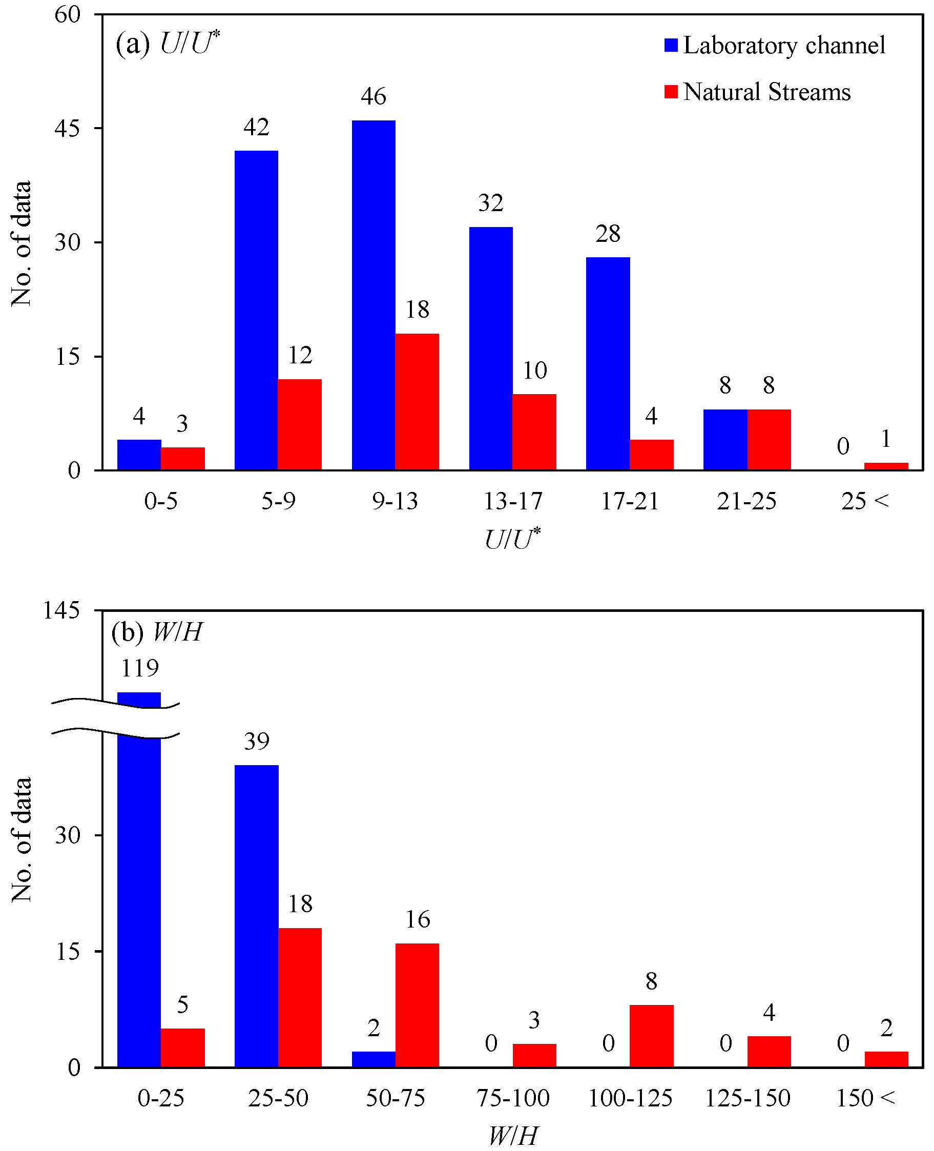
Figure 1. Distribution properties of the tracer test datasets according to the ranges of W / H .
Water 16 01359 g001aWater 16 01359 g001b
Figure 2. Research outlines to estimate transverse dispersion coefficient.
Water 16 01359 g002
Figure 3. Resampling results using oversampling techniques.
Water 16 01359 g003aWater 16 01359 g003b
Figure 4. Comparisons of the prediction results of D T / H U * using empirical formulas.
Water 16 01359 g004
Figure 5. Comparisons of the prediction results of D T / H U * using nonlinear regression methods. The dashed line indicates the best-fit to the measurements.
Water 16 01359 g005aWater 16 01359 g005b
Figure 6. Reproducible range of empirical formulas for estimating the transverse dispersion coefficient: red, blue, and green areas represent the available ranges using empirical formulas derived from original data, resampled data by ADASYN, and Jeon et al. [10], respectively.
Water 16 01359 g006
Figure 7. Comparisons of D T / H U * estimation results according to selection of the number of variables.
Water 16 01359 g007
Table 1. Statistical properties of collected tracer test results.
Laboratory Channels
(No. of Datasets = 160)
Natural Streams
(No. of Datasets = 56)
W / H U / U * D T / H U * W / H U / U * D T / H U *
Max65.124.60.70169.525.71.21
Min0.11.60.0514.43.70.12
Average17.712.50.1667.912.80.51
Median14.711.90.1457.411.00.49
Standard Deviation12.84.90.0740.36.00.24
Table 2. Empirical formulas for estimating transverse dispersion coefficient.
ReferencesEmpirical FormulasMethod
Yotsukura and Sayre [70] D T H U * = 0.4 U U * 2 W R c 2 MLR
Bansal [50] D T H U * = 0.002 W H 1.498
Deng et al. [17] D T H U * = 0.145 + 1 3530 U U * W H 1.38
Jeon et al. [10] D T H U * = 0.03 U U * 0.46 W H 0.3 S n 0.73
Baek and Seo [18] D T H U * = 77.88 P 2 1 e x p 1 77.88 P , P = U U * H R c
Gond et al. [12] D T H U * = f λ + 2.6 κ 3 U U * W H ,
f λ = 0.13   ( λ = 8 U U * > 0.08 ) , κ : flow nonuniformity parameter
Aghababaei et al. [19] D T H U * = 0.463 + 0.464 U / U * + 8.824 × 10 9 S n U / U * + 0.149 S n U U * + 2.306 F r S n 2 25.283 0.474 S n 0.054 W H 20.371 Genetic-programming-based symbolic regression (GP-SR)
Huai et al. [30] D T H U * = 0.693 262 + U U * 2 31.8 U U * + 0.121 W H W H + 0.222 U U * 1.99 (straight flume)
D T H U * = 0.693 U U * 0.47 262 + U U * 2 31.8 U U * + 0.121 W H 1.07 U U * 0.35 S n 0.395 W H + 0.222 U U * 1.99 (natural streams)
Genetic programming
(GP)
Table 3. Comparisons of oversampling techniques.
TechniqueData ResamplingProsConsReference
SMOTEGenerates synthetic samples near minority instancesMitigates class imbalanceSensitive to noisy dataChawla et al. [34]
SMOTE-ENNApplies Edited Nearest Neighbor (ENN) for noise reductionEffective in handling noisy dataPossible to discard informative instances during undersamplingBatista et al. [42]
ADASYNUtilizes density distribution for minority class data synthesisAdapts to data density variationsPossible to introduce noise due to adaptabilityHe et al. [41]
SVM-SMOTEIntegrates with support vector machine (SVM) for minority data synthesisGenerates samples in the feature space of minority classComputationally expensive and sensitive to SVM parametersNguyen et al. [78]
Table 4. Performance evaluations of the oversampled samples.
OversamplingClassification Performance IndicatorsKolmogorov–Smirnov Test: p-Value
Accuracy
(Equation (8))
Precision
(Equation (9))
Recall
(Equation (10))
F1
(Equation (11))
AUC * W / H U / U * D T / H U * Average
SMOTE0.8260.9370.8840.9100.9830.9920.9880.9790.986
SMOTE-ENN0.8200.9390.8740.9050.9830.9880.9600.9940.981
ADASYN0.7490.9310.8060.8640.9710.8890.5950.7830.756
SVM-SMOTE0.7630.9370.8150.8720.9690.8460.8330.9540.878
Note: * AUC = Area under the receiver operating characteristic (ROC) curve: this metric evaluates the performance of an oversampling model.
Table 5. Empirical coefficients obtained from the multiple linear regression.
DataCoefficients
abc
Original0.04430.44300.1228
SMOTE0.03230.36480.4055
SMOTE-ENN0.04080.36520.3118
ADASYN0.03520.44370.2348
SVM-SMOTE0.05580.40210.1273
Note: a, b, and c are empirical coefficients for an empirical formula, D T / H U * = a W H b U U * c .
Table 6. Comparisons of prediction errors resulted from empirical formulas.
This StudyPrevious Studies
Original DataSMOTESMOTE-ENNADASYNSVM-SMOTEBansal [50]Deng et al. [17]Jeon et al. [10]Aghababaei et al. [19]Huai et al. [30]
MAPE (%)53.467.365.757.263.0108.8155.451.227.015.0
MAPE (%) ( W / H 50 )56.4 73.8 71.6 61.2 67.9 80.8 131.7 55.5 27.7 15.0
MAPE (%) ( W / H > 50 )37.1 31.2 33.0 35.0 36.4 262.5 285.5 23.9 22.2 14.9
Table 7. Comparisons of prediction errors resulted from nonlinear regression methods.
DataData RangeMAPE (%)AverageRank
SVRXGBoostKNR
Original DataTotal44.144.342.243.65
W / H   5044.449.244.246.0
50 < W / H 42.517.331.330.4
SMOTETotal24.318.031.624.63
W / H   5027.919.332.726.7
50 < W / H 4.510.925.013.5
SMOTE-ENNTotal24.818.233.425.54
W / H   5028.519.134.427.3
50 < W / H 4.313.428.015.2
ADASYNTotal21.510.930.220.91
W / H   5024.411.031.622.4
50 < W / H 5.610.222.412.7
SVM-SMOTETotal22.516.532.923.92
W / H   5025.918.134.126.1
50 < W / H 3.57.725.912.4
Table 8. Comparisons of prediction errors according to the number of variables.
Original Data—MLROriginal Data—XGBoostADASYN—XGBoost
W / H ,   U / U * W / H ,   U / U * ,   S n W / H ,   U / U * ,   S n W / H ,   U / U * W / H ,   U / U * ,   S n
MAPE (%)54.238.0 15.712.49.5
Performance
Improvement (%)
-29.871.177.182.4
Disclaimer/Publisher’s Note: The statements, opinions and data contained in all publications are solely those of the individual author(s) and contributor(s) and not of MDPI and/or the editor(s). MDPI and/or the editor(s) disclaim responsibility for any injury to people or property resulting from any ideas, methods, instructions or products referred to in the content.