Investigating Nonpoint Source and Pollutant Reduction Effects under Future Climate Scenarios: A SWAT-Based Study in a Highland Agricultural Watershed in Korea

Abstract

This study investigated the effects of nonpoint source (NPS) pollution reduction and pollutant dynamics in a highland agricultural watershed in Korea. We employed the SWAT model to simulate hydrological processes and pollution transport within the watershed. The model incorporates future climatic scenarios derived from downscaled climate projections to assess their impacts on NPS pollution and pollutant reduction methods. These changes lead to heightened surface runoff and erosion rates, resulting in elevated sediment and nutrient concentrations. The projection indicates an anticipated increase in the annual average temperature by 1.3 to 2.1 °C by the mid-century, under scenarios SSP126 and SSP585. Additionally, precipitation levels are projected to increase by 31 to 61 mm from the baseline to the end of the century. Variations in hydrological components such as evapotranspiration, streamflow, and soil moisture are expected to range from +3.2 to +17.2%, −9.1 to +8.1%, and 0.1 to 0.7%, respectively, during the years 2040 and 2080. Fluctuations in TN, SS, and TP loading are estimated to range from −4.5 to +2.3%, −5.8 to +29.0%, and +3.7 to +17.4%, respectively. This study emphasizes the importance of adaptive management options for stakeholders and the need for adaptive management options to reduce nonpoint source pollution and protect water quality to maintain sustainable water supplies and conserve the environment in this watershed.

1. Introduction

Agricultural nonpoint source (NPS) pollution is a global issue that is primarily generated by local agricultural activities [1,2]. According to data, NPS contamination has harmed 30–50% of surface water sources, making it an increasingly serious threat to water quality and aquatic ecosystem restoration [3]. Every year, approximately 0.3–0.8% of cropland worldwide is impacted by severe deterioration, rendering the soil unsuitable for agricultural production [4,5]. Concerning this, NPS pollution has emerged as the primary contributor to water pollution in many Korean rivers and lakes, leading to the degradation of water quality [6]. Furthermore, pollution from agricultural NPS, specifically Total Nitrogen (TN) and Total Phosphorus (TP), has posed significant challenges to sustainable development in Korea [7]. The interplay of land use and climate change has a pivotal role in influencing water quality through NPS pollution pathways [8]. Climate change also exerts profound effects on watershed hydrology, altering chemical and physical processes, pollutant transport and transformation, and the capacity of water bodies to dilute pollutants [9,10]. These changes present new challenges for the management of watershed environments [6,11]. Furthermore, land use has a significant impact on pollutant formation and transport, influencing the key parameters that govern watershed runoff and soil erosion processes [12,13,14].

Recent studies investigated the effects of climate change on watersheds, using a variety of models such as the Soil and Water Assessment Tool (SWAT) mathematical approaches and hydrological climate models [15,16,17]. For instance, SWAT has been used to assess the reduction in high-level NPS pollution discharge from agricultural catchments in the highlands [18,19], and methodologies have been proposed to quantify future changes in the best management practices for controlling TP loads in river systems in response to climate change [20,21]. Therefore, the prediction of future climate change using the Coupled Model Intercomparison Project 6 (CMIP6) model and climate scenarios is an important task, and CMIP6 has been widely used in various fields in recent years to address these important challenges [22].

Over the past two decades, the Doam-dam watershed has seen a significant reduction in observed discharges due to both anthropogenic activities and the effects of climate change. The rise in temperature and decrease in surface water by 25–45% in Korea have posed serious threats to water supplies and environmental sustainability [23]. Several studies have focused on pollutant changes and improving water quality in Doam Lake [6,24,25], but only a few have looked at the impact of climate change on streamflow for the watershed scale. Furthermore, a water quality study cannot be undertaken without considering hydrological variability [26]. The key goals of this research are to analyze trends in NPS pollution in the study area, project the impact of climate change on NPS pollution and discharge patterns, and determine the distinctive characteristics of these phenomena. Furthermore, this study intends to support future climate change studies, assist in more effective water resource management, and facilitate adaptation planning in the Doam watershed and other similar places in Korea and globally.

This study significantly advances current understanding by systematically investigating the effects of climate change on water availability, nonpoint source (NPS) pollution, and nutrient dynamics in the Doam watershed. Further, this research reveals subtle insights regarding NPS pollution reduction by utilizing the SWAT model and including downscaled climate projections. This methodological fulfillment, which focuses on previously unstudied components of NPS pollution mitigation techniques, makes a significant contribution. The results emphasize the complex interplay between future climate scenarios and hydrological processes, underlining the importance of proactive water management techniques.

2. Materials and Methods

2.1. Study Area and Input Data

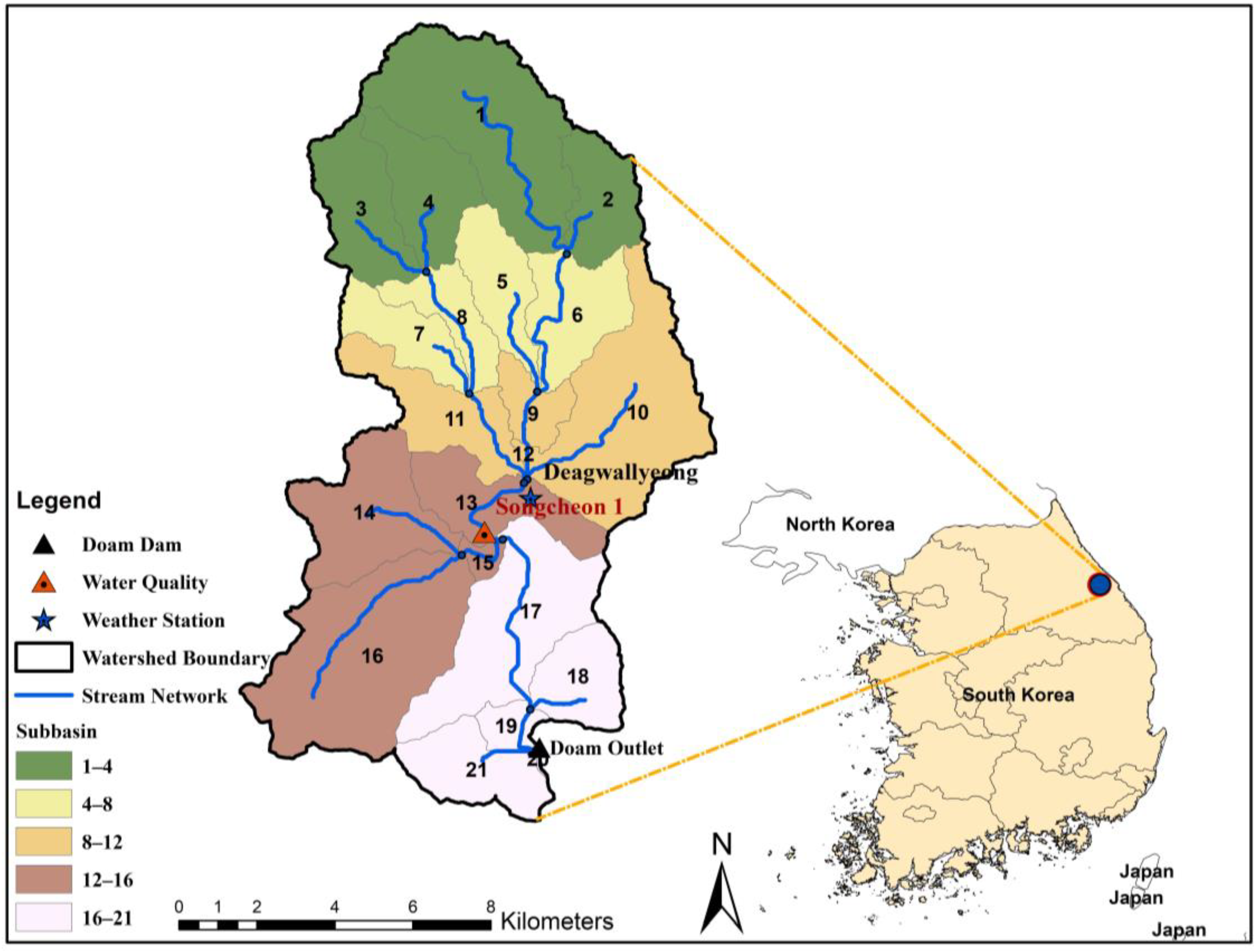
The Doam watershed spans an area of 151.2 km² with a channel length of 22.72 km and is situated at coordinates 38°35′–38°47′ N and 128°37′–128°47′ E (Figure 1). In this area, the annual precipitation averages 1693.03 mm, the mean temperature stands at 20 °C, and humidity reaches 82%. Vegetation predominantly comprises 79% forest and grassland, with arable land making up approximately 19% of the total. The primary vegetation types include deciduous forests cover 41.35% of the total area, followed by forest-evergreen forests at 15.96% and bermudagrass at 13.26%. Due to mountainous conditions, the topography is described as steeply sloping, a predominant land slope that falls within the 25 to 40% range, with altitudes ranging from 725 to 1455 m above sea level. The watershed’s dominant soil types are lithosols (neutral or alkaline rock) and grey soil or alluvial soil. Therefore, once the aforementioned finding is obtained and the result of the utilized data is acquired, we will apply the observational and weather data as follows:

Several essential datasets and inputs were utilized to run the SWAT model effectively for our study. These inputs encompassed weather data, thematic data including digital elevation models (DEM), soil type and land use data, and hydrological information. Daily weather data, from the monitoring station (Deagwalyeoung station), including parameters like precipitation, wind speed, relative humidity, sun radiation, and maximum and minimum temperatures, spanning the period from 2010 to 2020, were sourced from the Korea Meteorological Administration. These weather data records were indispensable for accurate model simulations. To delineate streams, and watersheds, and establish the longest possible flow path of streams during the floods, a high-resolution DEM with a 5 × 5 m resolution was obtained from the South Korean National Geographic Information Institute. This DEM served as the fundamental geospatial dataset for our analysis. The soil inputs essential for the SWAT model were derived from values provided in the soil texture map from the South Korean Soil Information System. These values were classified using classification charts from the United Nations Food and Agricultural Organization and the United States Department of Agriculture, supported by the SWAT soil database. Lastly, monthly streamflow and water quality data were retrieved from the South Korean Water Resources Management System and the Water Information System for model calibration and validation. Loads for model calibration and validation are calculated by multiplying the values of water quality parameters by the corresponding flow data simultaneously. These data spanned from January 2010 to December 2020, providing crucial information for assessing and refining the SWAT model’s performance.

2.2. SWAT Model

2.2.1. Hydrological and Water Quality Modeling

The SWAT model is a widely used hydrological model developed to simulate the movement of water, sediment, and various pollutants in a watershed. It is readily used to study the long-term effects of land management practices, climate variability, and land use changes on hydrological progress [27,28]. The SWAT setup is divided into watershed delineation, hydrological response unit (HRU) definition, and input table creation. The input data of the SWAT model were applied at various detailed levels, including the watershed, sub-watershed, and HRUs. The water balance was calculated at the HRU level, segmented at the sub-watershed level, and then routed to the reaches and watershed outlet. The hydrologic cycle simulated by SWAT is based on the water balance equation as follows:

$${\mathrm{S}\mathrm{W}}_t={\mathrm{S}\mathrm{W}}_0+{\sum }_{i=1}^t\left({\mathrm{R}}_{day}-Q_{surf}-{\mathrm{E}}_a-{\mathrm{W}}_{seep}-{\mathrm{Q}}_{gw}\right)$$

(1)

where ${\mathrm{S}\mathrm{W}}_t$ is the final soil water content (mm), ${\mathrm{S}\mathrm{W}}_0$ is the initial soil water content on day I (mm), t is the time (days), ${\mathrm{R}}_{day},Q_{surf},{\mathrm{E}}_a$ represent the precipitation, surface runoff, and amount of ET on day I (mm), ${\mathrm{W}}_{seep}$ is the measure of water entering the vadose zone from the soil profile on day I (mm), and ${\mathrm{Q}}_{gw}$ is the measure of groundwater discharge on day I (mm).

The sediment yield is one of the critical parameters considered for this research. Sediment yield is computed in the SWAT model using the Modified Universal Soil Loss Equation (MUSLE) and the Revised Universal Soil Loss Equation (RUSLE), which consider factors such as slope, land use, and soil properties into account to estimate soil erosion and sediment yield [29,30]. The daily sediment yield can be calculated as follows:

$$Sed=11.8\times {\left(Q_{surf}\times q_{peak}\times {Area}_{hru}\right)}^{0.56}\times K_{USLE}\times C_{USLE}\times P_{USLE}\times {LS}_{USLE}\times CFRG$$

(2)

where $Q_{surf}$ is the surface runoff volume (mm/ha), $q_{peak}$ is the peak runoff rate (m³/s), ${Area}_{hru}$ is the area of the HRU (ha), $K_{USLE}$ is the Universal Soil Loss Equation (USLE) soil erodibility factor (0.013 metric ton m² hr/(m³-metric ton cm)), $C_{USLE}$ is the USLE cover and management factor, $P_{USLE}$ is the USLE support practice factor, ${LS}_{USLE}$ is the USLE topographic factor, and CFRG is the coarse fragment factor.

We continued with the calibration and validation of the dataset after the simulation and acquisition of SWAT data. The SWAT model was calibrated using data from the Songcheon#1 watershed daily observed streamflow, as well as monthly TN and TP. The model simulation was run for seven years, with datasets from 2013 to 2018 utilized for calibration and those from 2019 to 2020 for validation. Therefore, the two statistical metrics, the Nash-Sutcliffe efficiency (NSE) index and R2, were used to evaluate the effectiveness of the SWAT model simulation. Equations (3) and (4) were used to obtain the NSE index and coefficient of determination (R2) values, respectively.

$$\mathrm{N}\mathrm{S}\mathrm{E}=1-\frac{{\sum }_{i=1}^N({\mathrm{Q}}_{\mathrm{s},\mathrm{i}}-Q_{\mathrm{o},\mathrm{i}}{)}^2}{{\sum }_{i=1}^N({\mathrm{Q}}_{\mathrm{o},\mathrm{i}}-{\overline{Q}}_{\mathrm{o}}{)}^2}$$

(3)

Here, N is the number of observations, ${\mathrm{Q}}_{\mathrm{s},\mathrm{i}}$ is the simulated value at time i, ${\mathrm{Q}}_{\mathrm{o},\mathrm{i}}$ is the observed value at the time i, and ${\overline{Q}}_{\mathrm{o}}$ is the mean observed streamflow. NSE values vary from −∞ to 1, with 1 being the optimal number.

$$R^2=\frac{{\left[{\sum }_{i=1}^N\left({\mathrm{Q}}_{\mathrm{o},\mathrm{i}}-{\overline{Q}}_{\mathrm{o}}\right)\left({\mathrm{Q}}_{\mathrm{s},\mathrm{i}}-{\overline{Q}}_{\mathrm{s}}\right)\right]}^2}{{\sum }_{i=1}^N{\left({\mathrm{Q}}_{\mathrm{o},\mathrm{i}}-{\overline{Q}}_{\mathrm{o}}\right)}^2{\left({\mathrm{Q}}_{\mathrm{s},\mathrm{i}}-{\overline{Q}}_{\mathrm{s}}\right)}^2}$$

(4)

Here, ${\overline{Q}}_{\mathrm{s}}$ is the simulated flow.

The reference period in this study refers to the historical simulation period from 1981 to 2010, and the future evaluation period is divided into three time periods (2011–2040, 2041–2070, and 2070–2100). Future climate scenario data were input into the calibrated SWAT model, which simulates NPS pollution in the watershed under various climate change scenarios. The characteristics of the change in the output of NPS pollution over different future assessment periods were evaluated by comparison with the reference period.

2.2.2. Hydrological Model Setup and Data Preparation

Model Setup

The SWAT model was used in this study to do a detailed hydrological analysis across 21 sub-basins using USGS National Elevation Datasets (NED) 5 × 5 m resolution DEM and Deagwalyeoung meteorological data. The combination of several datasets and methods, including the Penman-Monteith and CN methods, was used to accurately convey the complexities of hydrological processes [27,31,32].

Parameter Sensitivity Analysis and Calibration

A parameter sensitivity study utilizing inclusive probability uncertainty estimation was performed using the SWAT CUP program focusing on the parameters that have a significant influence on streamflow and sediment load projections, aligning with the approach proposed [33,34]. Subsequently, we calibrated the SWAT model using the aforementioned parameters and harnessed the non-dominated sorting genetic algorithm II (NSGA-II) method, as detailed by [35]. This calibration effort was centered on establishing a strong correlation between the model’s average daily simulated streamflow and observed data. We used the freely available NSGA-II Python tool built for SWAT model calibration, as presented by [36] for the calibration process. We chose the watershed outlets as objective sites to improve the model’s performance evaluation, using the NSE proposed by [37] and the percent bias (PB) as criteria for assessing the goodness of fit regarding simulated streamflow. Calibration with NSGA-II focused on watershed outflows, with NSE, PB, R2, and RSR criteria utilized to evaluate model performance [38]. The Doam outflow gauge’s observed daily flow data (2016–2020) was important in this calibration process.

Lastly, the SWAT model was calibrated to identify years with significant runoff changes in each subbasin [39,40]. This understanding is critical for dealing with the environmental, economic, and societal implications. To analyze runoff changes from 2012 to 2020, statistical approaches were used such as the Mann–Kendall (M–K) method [41], sliding t-test [42], and cumulative anomaly test [43].

2.3. Climate Change Scenarios and Future Climate Changes

General circulation models (GCMs) predict climatic conditions by integrating interconnected Earth system models that involve numerous components, including the atmosphere, liquid and solid water bodies, and Earth’s surface [44]. Given that each model’s emission scenario within a model yields several different future projections, it shows that the integration of numerous GCMs along with multiple emission scenarios can create a collaborative modeling approach, this collective setting helps to explain a precise and suitable spectrum of future projections [45,46].

Table 1. Information about the global climate models (GCMs) used in this study.

No	Model	Resolution	Modeling Group	References
1	CanESM5	2.81° × 2.81°	Canadian Centre for Climate Modelling and Analysis.	[48]
2	ACCESS-CM2	1.875° × 1.25°	Commonwealth Scientific and Industrial Research Organization in collaboration with the Queensland Climate Change Centre of Excellence.	[49]
3	GFDL-ESM4	1.25° × 1.00°	Geophysical Fluid Dynamics Laboratory.	[50]
4	UKESM1-0-LL	1.875° × 1.25°	Met Office Hadley Centre.	[44]
5	INM-CM4-8	2.00° × 1.50°	Institute for Numerical Mathematics Japan Agency for Marine-Earth Science and Technology, Atmosphere and Ocean Research Institute, and National Institute for Environmental Studies.	[51]
6	MIROC6	2.81° × 2.79°		[52]
7	BCC-CSM2-MR	1.13° × 1.13°	Beijing Climate Center (BCC) and China, Meteorological Administration Beijing Climate Center climate system model.	[53]

provides detailed information on the models used in this study, including their resolutions, classification, and model group information. A simple quantile mapping (SQM) downscaling method was used for downscaling and bias correction [47]. We used a combination of statistical downscaling methods, including the World Climate Research Programme (WCRP), the CMIP6 multi-model, and localized constructed analog (LOCA) downscaled CMIP6 daily climate projections, to achieve our results. These methods were used to extract acceptable analog days from observational data.

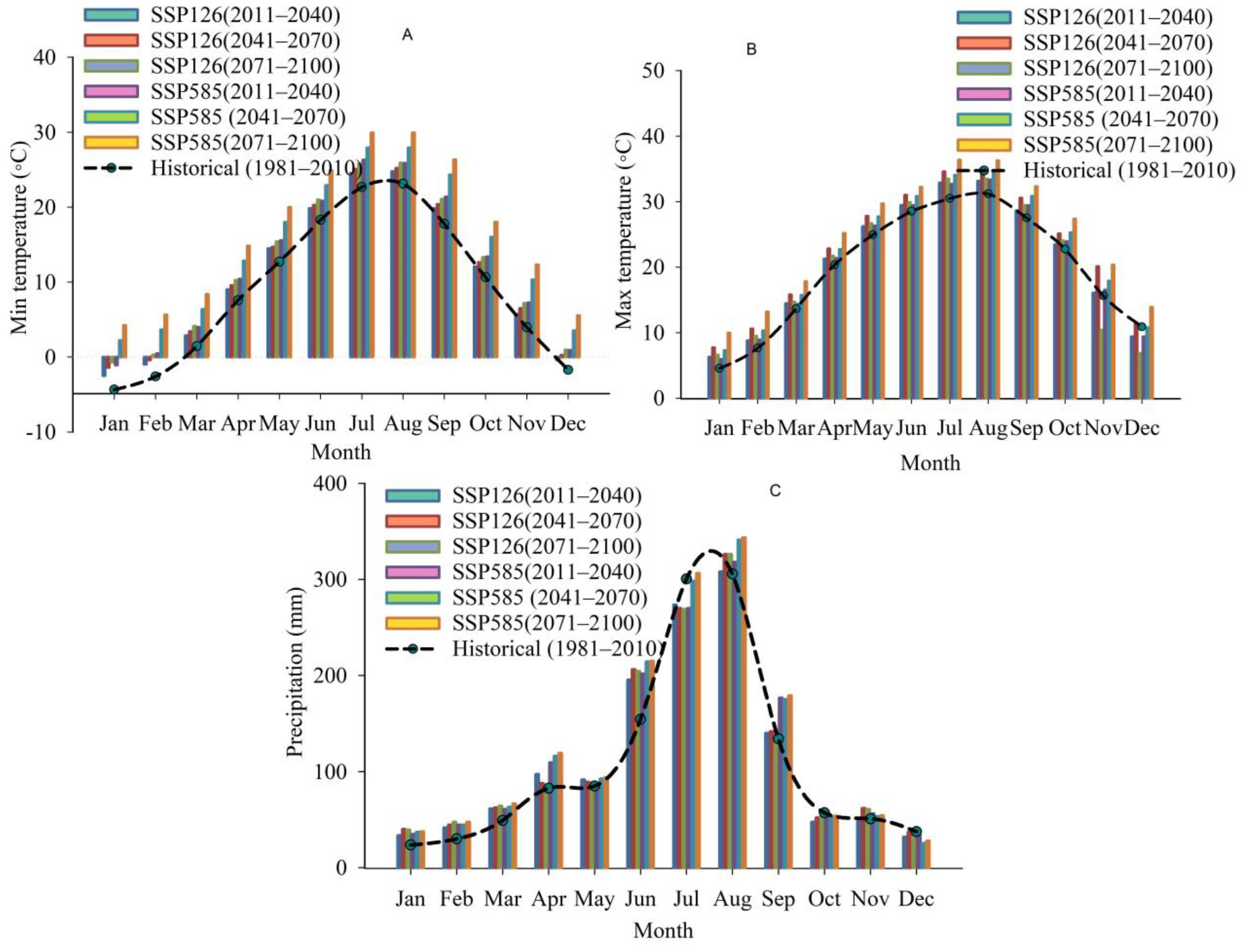
Our finding revealed that during the first period (2011–2040) under SSP126 and SSP585, the annual average of daily maximum and minimum temperatures are anticipated to rise by 2.57 and 2.8 °C and 2.57 and 2.85 °C relative to the baseline (1981–2010), respectively. Under the two climate change scenarios, the annual average of the daily maximum temperatures is projected to increase by 4.57 and 7.23 °C and 11.41 and 12.27 °C and the daily minimum temperatures by 4.6 and 7.58 °C and 4.9 and 12.69 °C, respectively, from the baseline for the second periods (2041–2070 and 2071–2100). The annual average precipitation is projected to change by 165.97 and 139.68 mm and 200.14 and 241.04 mm from the baseline during 2011–2040 and 2041–2070 under SSP126 and SSP585, respectively, in

Table 2. The projected annual changes in the daily maximum/minimum temperature and annual precipitation at the Deagwalyeoung weather station.

Climate Variable	Baseline 1981–2010	Scenario	2011–2040		2041–2070		2071–2100
			Sim. *	Diff. *	Sim.	Diff.	Sim.	Diff.
Annual average of daily max temperature (°C)	18.16	SSP126	20.73	2.57	22.73	4.57	29.57	11.41
		SSP585	20.96	2.8	25.39	7.23	30.43	12.27
Annual average of daily min temperature (°C)	3.76	SSP126	6.33	2.57	8.36	4.6	8.66	4.9
		SSP585	6.61	2.85	11.34	7.58	16.65	12.69
Annual precipitation (mm)	1821.39	SSP126	1987.36	165.97	2021.53	200.14	2032.61	202.22
		SSP585	1961.07	139.68	2062.43	241.04	2228.64	407.25

Note(s): * Sim. stands for simulation, and Diff. stands for difference.

.

Similarly, under the two climate change scenarios, the annual average precipitation is expected to increase by 202.22 and 407.25 mm between 2071 and 2100. These findings are summarized in Table 2, which shows that the annual average daily maximum and minimum temperatures and annual precipitation trends are similar to the respective monthly average trends. The average temperature and precipitation increased under both scenarios, with the most significant increases occurring in July and August. Whereas, under SSP126 and SSP585, the monthly average daily maximum and minimum temperatures are expected to rise sharply from 0.73 to 4.21 °C and 0.91 to 4.43 °C, respectively, in July and August (Figure 2A,B). The changes in monthly average precipitation are similar to those in temperature; precipitation increased significantly from 41.5 to 101.3 mm in July and August (Figure 2C). This indicates that precipitation is intense in summer. This indicates rising temperatures because warm air can evaporate more water into the atmosphere. As a result, more precipitation occurs naturally in air masses, with more water vapor available for precipitation. Our findings suggest an increase in temperature in the foreseeable future, as well as an increase in rainfall, particularly during the wet season, indicating the essential need for long-term management.

3. Results and Discussion

3.1. Sensitivity Analysis and Model Calibration and Validation

SWAT model is known to have a large number of parameters; the selection of the most sensitive parameters for a given watershed is the first phase in the calibration and validation process in SWAT [48]. The Latin hypercube one-factor-at-a-time category of sensitivity analysis resulted in 5 of the 15 hydrologic parameters being highly influencing significant factors

Table 3. The most sensitive parameters revealed meaningful effects on sediment.

Parameter	Variable Description	Default	Min	Max	Cali. Value
Flow	Baseflow Alpha (days)	0.048	0.001	1	0.8
	Groundwater Delay (days)	31	0.0001	500	63
	Evaporation Compensation	0.95	0.01	1	0.1
	Initial SCS Curve Number II	85	35	98	−0.5
	Available Water capacity (mm H2O/mm soil)	0.2	0.01	0.4	+0.05
Sediment	Channel erodibility	0.001	0.001	1	−0.02
	Sediment Concentration (lateral flow)	0.001	1	500	0
	USLE Support PracticeFactor	0.01	0.01	1	0.1
TN	Rate Factor Humus mineralization	0.003	0.001	0.001	0.001
	Residue Decomposition Factor	0.05	0.02	0.1	0.03
	Initial NO3 Concentration (soil layer)	0.01	0	100	0.9
	Biological Mixing Efficiency	0.2	0	1	0.5
TP	Phosphorus percolation Factor (10 m3 Mg−1)	10	10	17.5	13
	Organic P Enrichment Ratio	0.001	0	5	0.03
	Initial Organic P (mg P kg−1 soil)	0.01	0	100	14

. The soil conservation service runoff curve number (CN2), threshold water depth in the shallow aquifer for return flow to occur, groundwater delay time, channel erodibility factor, and baseflow alpha factor (days) were the most sensitive parameters. Similarly, the most sensitive parameters were the USLE support practice factor and USLE soil erodibility factor in the sediment, the initial NO3 concentration in the soil layer (SOL NO3) in the TN, and phosphorus soil partitioning coefficient in the TP. Table 3 shows a full overview of the most sensitive parameters used in our study, along with detailed descriptions and the compression method used. It also displays the calibrated values generated as a result of this examination. Several research studies have used sensitivity analysis techniques in hydrological modeling for calibration and validation. A Monte Carlo sensitivity analysis approach obtained critical parameters in one such investigation utilizing the HSPF model [54]. Another study used the Vflo^TM hydrological model for sensitivity analysis, using the Sobol approach to identify critical parameters for calibration and validation [55]. In both research studies, the initial abstraction ratio, recession constant for direct runoff, groundwater travel time, channel width exponent, and baseflow recession coefficient were all important hydrologic characteristics, along with sediment and nutrient modeling revealed the same pattern, with parameters such as sediment delivery ratio and phosphorus sorption rate playing critical roles in both investigations. Therefore, our findings show that the SWAT Cup provides high accuracy.

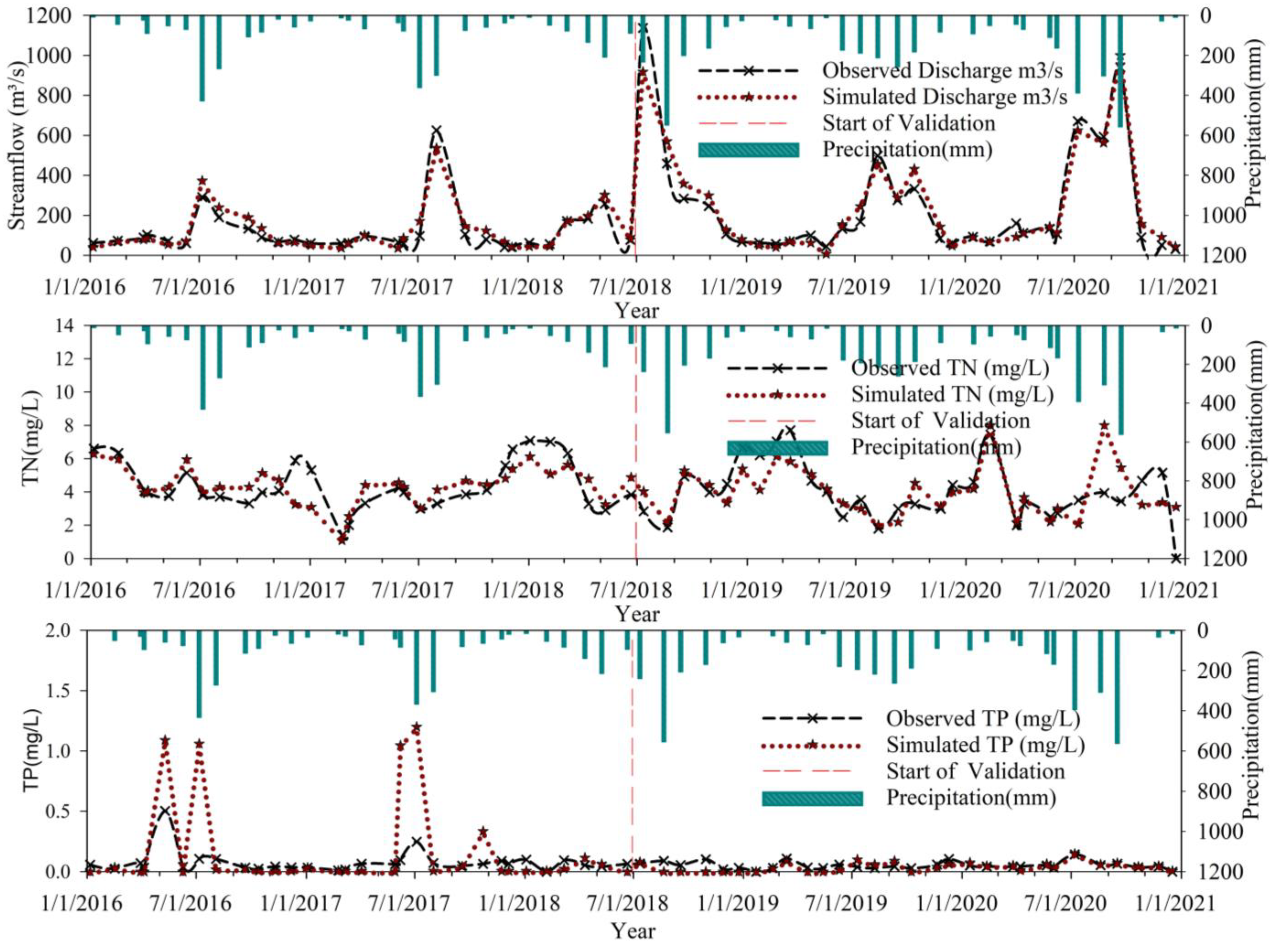
The analysis of the simulation data reveals several notable results. The R2, NSE, and PBAIS key performance indicators for streamflow attained values of 0.81, 0.95, and 0.018, respectively, over the calibration period. These indicators recorded values of 0.89, 0.82, and 0.015 during the validation period, indicating high model performance in simulating streamflow dynamics. Conversely, when evaluating water quality throughout the calibration period, the TN and TP load simulations showed R2 values of 0.54 and 0.498 for TN and TP, along with NSE values of 0.72 and 0.53, respectively (

Table 4. Performance metrics for streamflow and water quality simulations are coefficient of determination (R2), Nash-Sutcliffe Efficiency (NSE), and Percent Bias (PBIAS).

Station	Statistics	Flows (m3/s)		TN Loads (kg/day)		TP Loads (kg/day)
		Cali.	Vali.	Cali.	Vali.	Cali.	Vali.
Songcheon 1	R2	0.81	0.89	0.54	0.53	0.498	0.50
	NSE	0.95	0.82	0.72	0.71	0.53	0.78
	PBAIS (%)	0.018	0.015	0.205	2.93	1.93	2.93

Note(s): Calibration period (2016–2018) (Cali.); Validation period (2019–2020) (Vali.).

).

In general, a sufficiently accurate simulation result is given when the absolute value of NSE is positive, the absolute value of R2 exceeds 0.6, and the absolute value of PBAIS (%) is positive, as outlined in previous studies [56]. While not as strict, the standards for nutrient assessment require the absolute value of relative error to be less than 40%, the Nash coefficient to be greater than 0.5 [33], and R2 to fulfill the same limit as that used for runoff [56]. These criteria are met for both nitrogen and phosphorus simulations, confirming the improved model’s efficacy in furthering nonpoint source pollution modeling and analytical studies (Figure 3).

There are several factors for the observed differences in water quality performance measurements. First, the Songcheon#1 station is significantly impacted by upstream agricultural activities, which could be a factor in the model’s poor performance. It is important to remember that the CN method challenges predict runoff on days with several storm events, which could result in underestimations [32,33]. Additionally, the accuracy of the water quality simulations may have been influenced by the availability of missing data for both the calibration and validation periods. The water quality simulation values, especially during the calibration period, fell short of the expected benchmarks, even though the streamflow simulation findings satisfied a few flood events exclusion criteria for successful and satisfying model performance. These variations point out regions that need further improvement in upcoming modeling attempts and can be attributable to upstream agricultural impacts and data restrictions.

3.2. Runoff Variation Trend

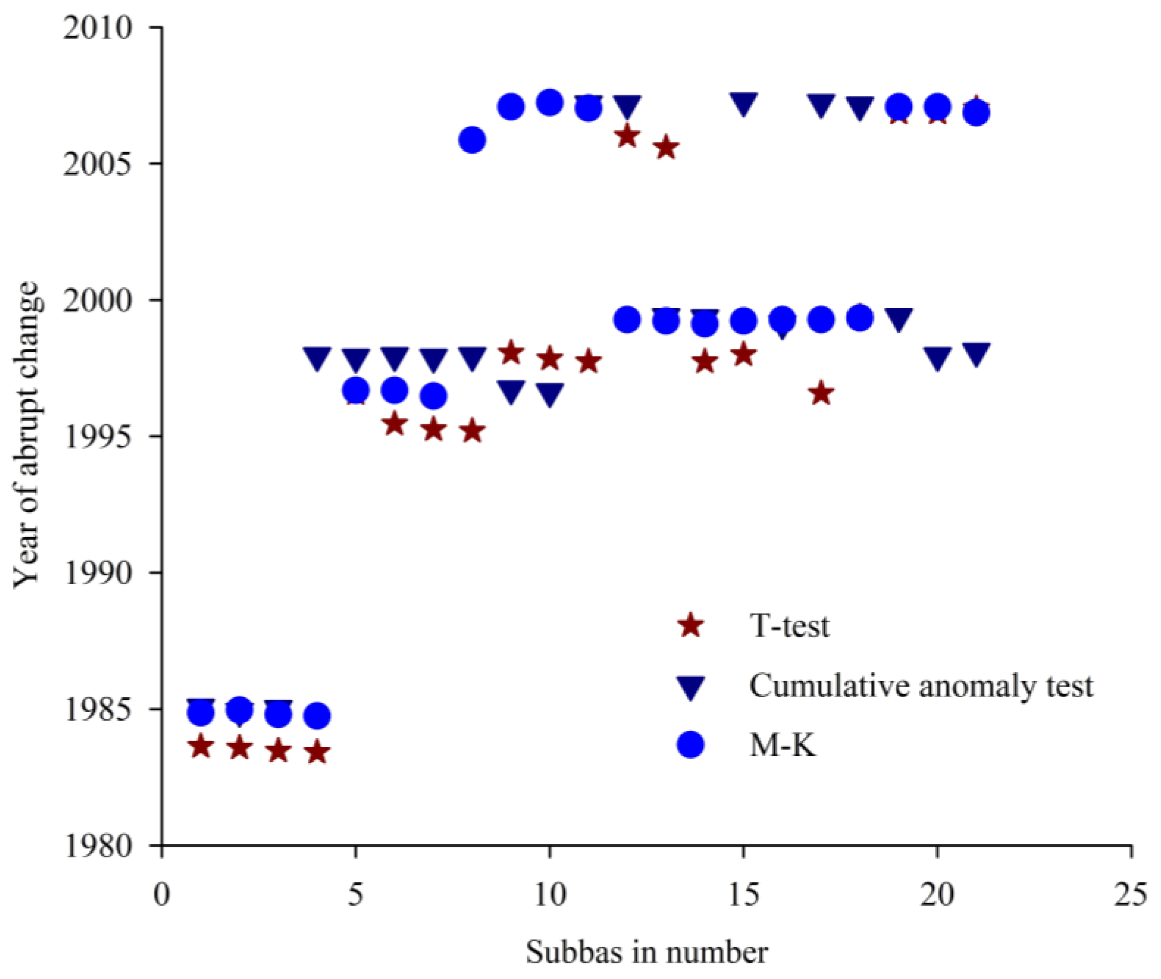
Using the SWAT model, we have successfully identified the years characterized by the most abrupt change in each subbasin. Figure 4 depicts the temporal variations in runoff for the river basins spanning from 1981 to 2010 as determined by the SWAT simulation results for each subbasin. When examining alterations within the sub-basins, the results of the three different approaches consistently identified significant changes in 2018, 2019, and 2020. Specifically, among the 21 sub-basins assessed, 7, 9, 16, and 17 exhibited significant variations during this period, whereas the remaining 17 sub-basins remained relatively stable (Figure 5). These variations can be attributed to a multitude of factors, including the complex and diverse geographical features such as the high mountainous terrain in the eastern areas and low basins and hills in the eastern regions. Furthermore, variations in land use, temperature, vegetation cover, and various meteorological factors may also contribute to the observed variances.

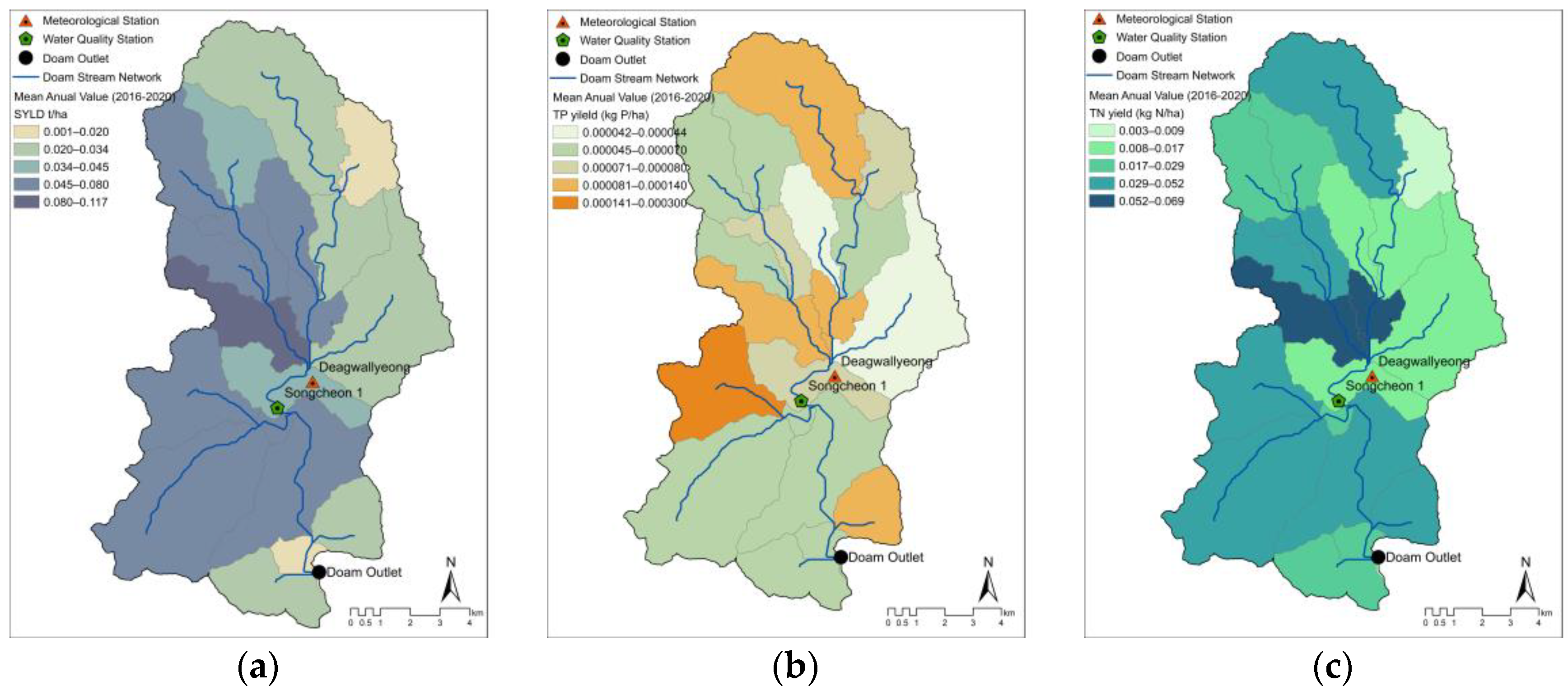
The spatial distribution of sediment, TN, and TP loading in watersheds is important for effective water management. Using the SWAT model, we have generated valuable insights into these parameters, as shown in Figure 5. The model’s information is useful in supporting sustainable practices within each basin area. The technique also promoted awareness of the watershed’s sediment output and NPS load. Subbasins 3, 7, 11, 14, and 16 have particularly high sediment severity, with NPS loads accounting for 33.42% of the total area. This shows that significant sediment accumulation is occurring in specific sub-basins of the watershed. These areas could possess distinct characteristics, such as steep topography or a high potential for erosion, which may contribute to the observed variances in sediment output. Sub-basin 11 has the greatest predicted yearly average sediment yield of 0.117 t/h/yr, indicating that localized factors are strengthening sediment movement within that sub-basin. High-intensity rainfall events, soil types, or land use practices that encourage erosion are examples of such factors. The cumulative impacts of sediment buildup and transit from various sub-basins may influence the overall annual sediment output of 18.5 t/yr for the entire watershed. The difference between the simulated output (0.117 t/h/yr) and the total annual sediment output (18.5 t/yr) could be attributed to model limitations, spatial resolution, or simplifications taken in simulating complicated hydrological processes. The accuracy of input data and assumptions used for the modeling process may limit the model’s capacity to capture small-scale differences in sediment transport.

Watersheds will change significantly in the future, with an increasing trend from 2071 to 2100, depending on the evaluation period, emission scenarios, and global climate models. Between 2041 and 2070, the CanESM5 SSP585 scenario shows an increase in runoff and TP, but TN shows a declining trend. Sub-watersheds with a high potential for pollution growth are mostly found in the lower parts. Therefore, dam management must evaluate annual changes in each basin as well as detect sediment production levels in each basin for managing pollutant production reduction through erosion control, flow management during periods of high sedimentation, and trapping and removing sediments in reservoirs using various approaches, such as afforestation on steep slopes, the establishment of vegetative buffers along watercourses, and the installation of erosion control structures such as silt barriers and check dams, and lastly regularly monitor weather forecasts and hydrological factors to anticipate high sedimentation periods. When substantial rainfall or snowmelt is forecast, they proactively adjust dam release rates to build additional storage capacity in the reservoir. These measures will contribute to stabilizing the soil, erosion prevention, and sediment reduction in the reservoir, along with regular monitoring, ensuring that these erosion control methods are effective.

Our findings are consistent with those of a study that used the HEC-HMS model to identify critical years marked by significant changes in each subbasin [57], unlike this study, identified important years highlighted by considerable changes in each subbasin by using the Mann–Kendall (M–K) method, sliding t-test, and cumulative anomaly test. Another study that used the LISFLOOD model, which normally models bigger areas such as river basins or continents, encountered difficulties in capturing small-scale changes in sediment transport [58]. We use the SWAT output database in our smaller-scale watershed, concentrating on the geographical distribution of sediment, TN, and TP loading in watersheds.

3.3. Analysis of Seasonal Variation of Runoff under Future Climate Changes Model

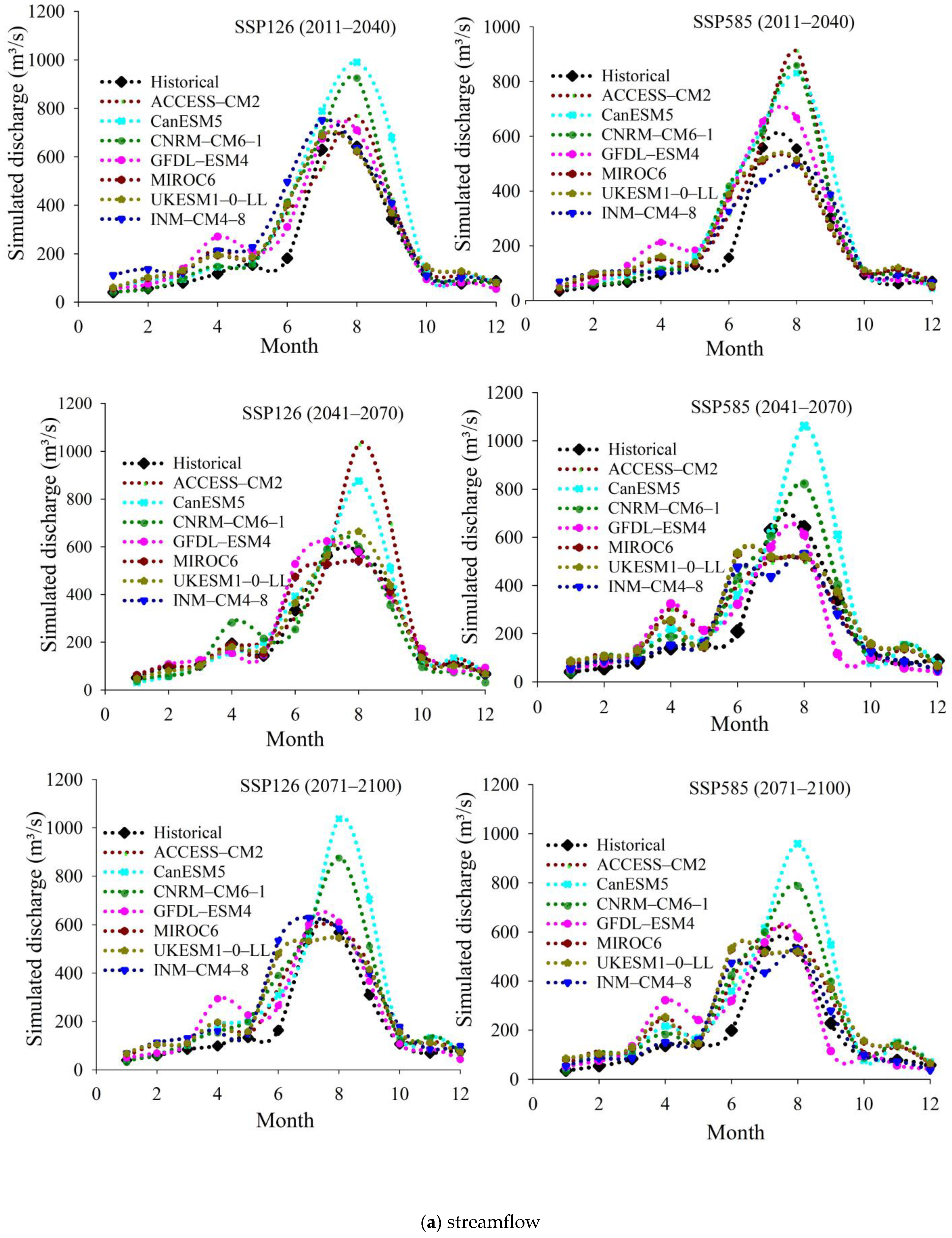
We chose to apply SSP126 and SSP585 scenarios using seven GCM models in Table 1 and future projection for three time periods (2011–2040, 2041–2070, and 2071–2100) using the baseline data (1981–2010) since they cover a wide range of anthropogenic radiative forcing, global CO2 concentrations, and emissions, giving a relevant picture of potential future climatic impacts depending on various socioeconomic pathways. 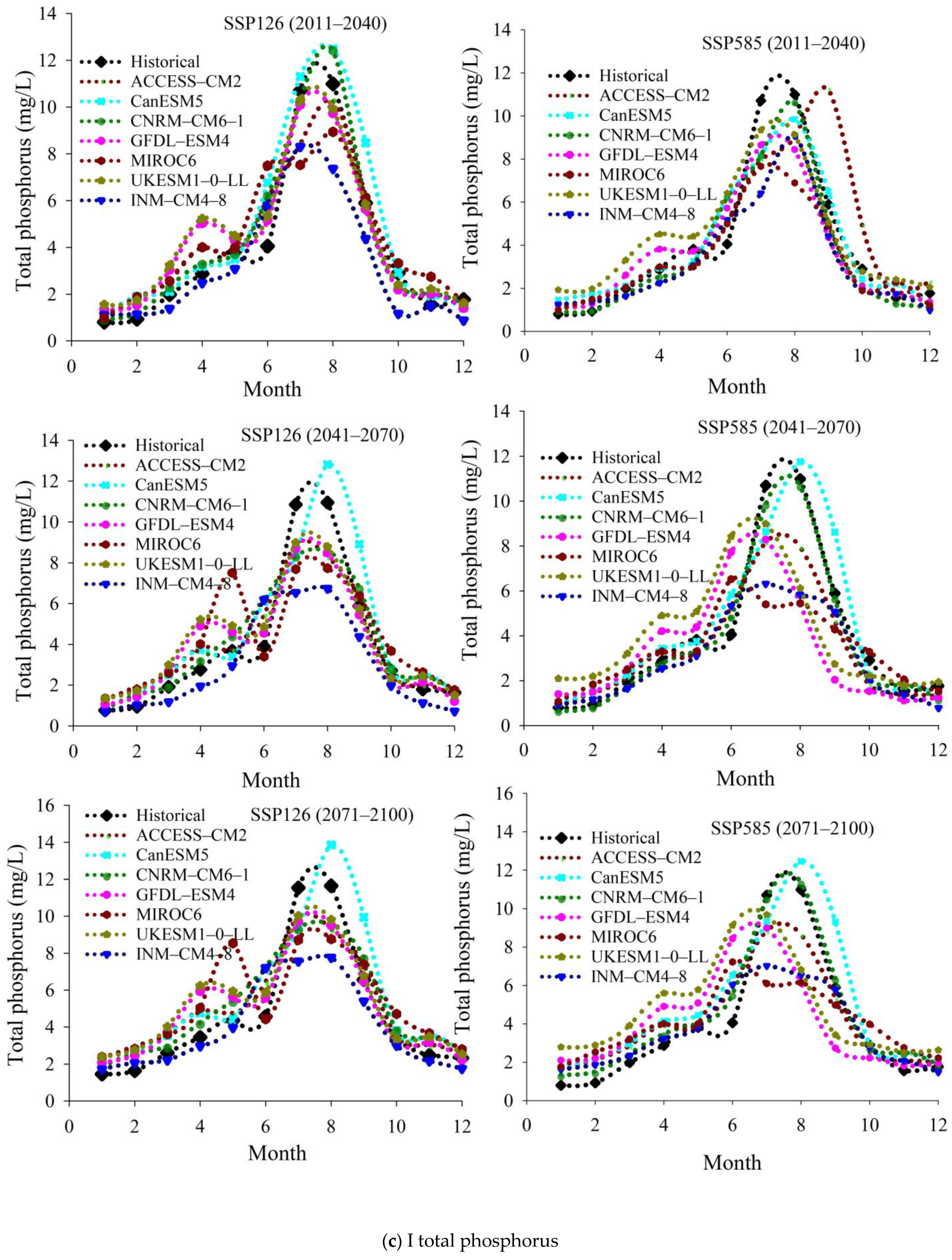Figure 6 shows dynamic shifts in the below scenario under SSP126 and SSP585, showing a continuous decrease in monthly discharge relative to historical values. However, there is cause for concern as maximum flow shifts to the wet season (July to September) in various climate models (ACCESS-CM2, CanESM5, CNRM-CM6-1, GFDL-ESM4, INM-CM4-8, MIROC6, UKESM1-0-LL), implying a collective response to changing climatic circumstances. This understanding provides insights into the possible influence of climate change on discharge patterns, but increases complications, particularly during the rainy season, providing issues for water management and ecosystem dynamics. Infrastructure and adaptability measures must be reconsidered.

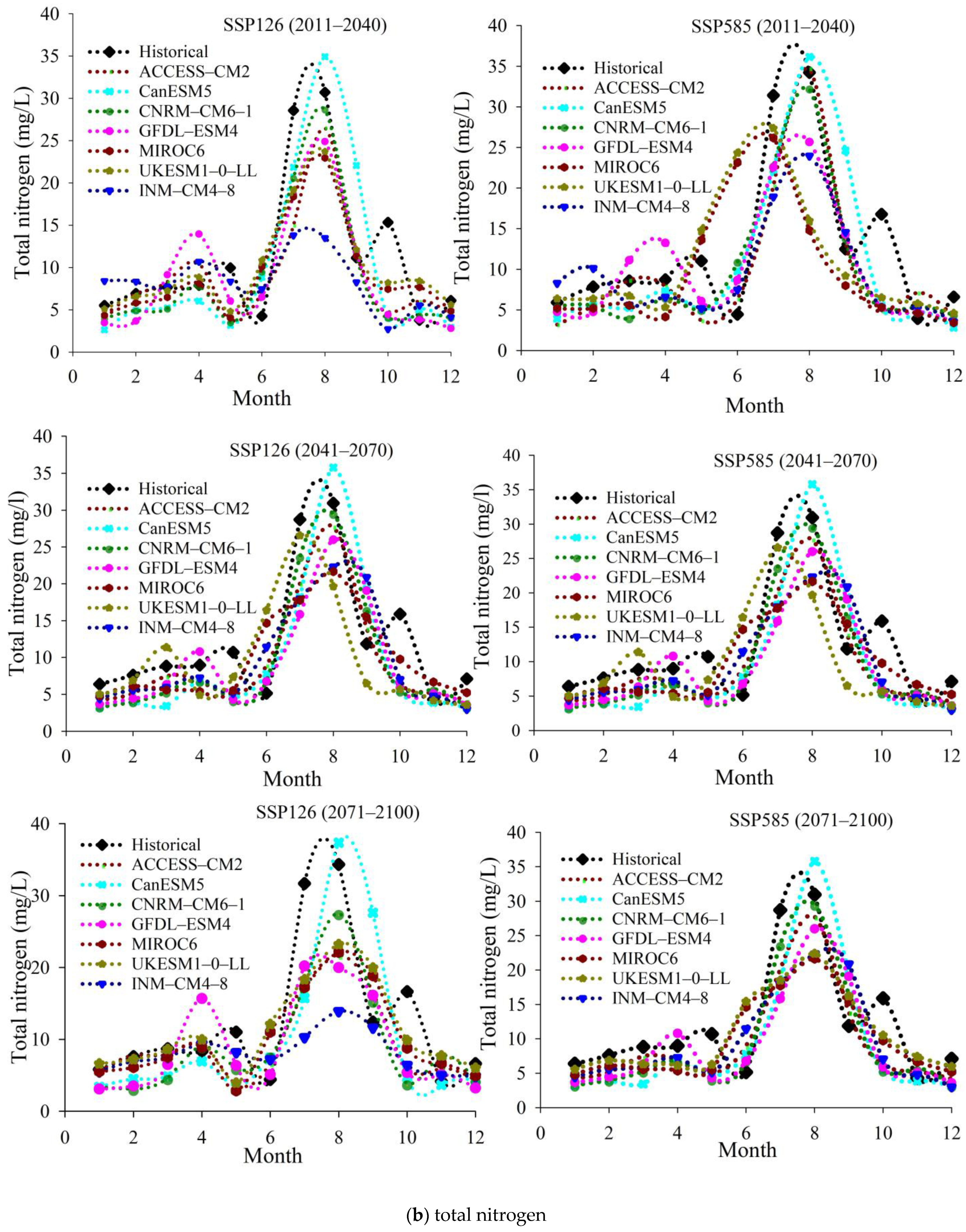
Assessing factors impacting total phosphorus (TP) and total nitrogen (TN) changes throughout various flow times under multiple climate models presents similar issues. Understanding the complex interplay of climate, land use, and other factors is critical for effective water resource management. Model evaluations using the Historical baseline demonstrate nuanced differences in TN and TP projections, emphasizing the importance of model-specific variables. Monthly variances reveal probable patterns of seasonality, which are critical for understanding temporal nutrient dynamics. Recognizing modeling uncertainties, such as sensitivity and data quality, is critical for improving predictions. Integrating data from TN and TP variations provides for a holistic approach to nutrient management, optimizing environmental conservation efforts. Previous study [57] emphasizes the need to take a comprehensive approach to adapting to changing climatic conditions, and Similar study measures indicating a constant drop in discharge values under comparable climate change scenarios, have validated our findings [59]. However, the effects of various factors on runoff were primarily concentrated during the high-flow period of the year. Precipitation changed runoff in most sub-basins (83.2%) during the high-flow period, and during the normal-flow period, changes in precipitation increased runoff in most sub-basins (79.9%). Precipitation had little effect on runoff during the low-flow period. This could be due to significant reductions in precipitation during the high-flow period owing to climate change in the study area. This finding indicated changes in runoff in the lower reaches of the Doam Basin during the normal flow period compared to during the high flow period (Figure 2). The effects of possible evapotranspiration on runoff were more significant during the high-flow period in 87.3% of the subbasins than during the normal- and low-flow periods.

In most basins, evapotranspiration increased during high, normal, and low-flow periods, whereas runoff changes caused by changes in potential evapotranspiration varied seasonally. This demonstrates that seasonal variations in precipitation in the study area significantly impact changes in runoff. In 98.9% of sub-basins, the effects of landscape changes on runoff were greater during the high-flow period than during the normal- and low-flow periods. However, the environmental and seasonal changes were minimal. The reason for these differences could be abundant precipitation during the high-flow period, which saturated the soil in the landscape and caused more runoff. Finally, the analysis of seasonal variation in runoff under future climate change highlights the role of precipitation, evapotranspiration, and landscape changes in driving changes in runoff patterns throughout the Doam watershed. Alamdari et al. [60,61] confirm the SWAT model’s accuracy and effectiveness in evaluating the impact of climate change on water quality and quantity by using downscaled climate projections to examine implications on water availability and quality. Similarly, the study led by Luo et al. [59], which projects climate change effects on water supplies and quality in a watershed, the current study forecasts temperature, precipitation, and hydrological patterns for the next century using global climate models expected to increase. This study also confirms the accuracy and efficacy of the SWAT model that we used in our research.

This collection of research strengthens the robustness and dependability of our observations, allowing us to gain a more complete knowledge of the effects of climate change on hydrological systems.

4. Conclusions

This study presents a slew of findings with profound implications for both watershed management and our understanding of the effects of climate change on hydrological systems. Our results reveal a clear and concerning trend of the rising annual average temperature of 1.3 to 2.1 °C by the mid-century under scenarios SSP126 and SSP585, along with significant shifts in annual precipitation, particularly during the wet season, ranging from 31 to 61 mm from the baseline to the end-of-century. Furthermore, variations in key hydrological components such as evapotranspiration, streamflow, and soil moisture range from +3.2% to +17.2%, −9.1% to +8.1%, and 0.1% to 0.7%, respectively, during the years 2040 and 2080. Importantly, variations in total nitrogen (TN), suspended solids (SS), and total phosphorus (TP) loading range from −4.5% to +2.3%, −5.8% to +29.0%, and +3.7% to +17.4%, respectively. This study includes a sensitivity analysis to identify the parameters that have the greatest influence on the watershed. We found the most sensitive parameters identified for hydrology were CN2, GWQMN, GW DELAY, CH EROD, and ALPHA_BF, while for nitrogen, USLE P, USLE K, SOL NO3, and PHOSKD were significant. As shown by high-performance measures (R2, NSE > 0.5), our modeling efforts yielded acceptable results resembling streamflow patterns. The findings regarding the variance in runoff patterns within sub-basins were observed in the years 2018–2019–2020, characterized by major alterations in runoff patterns. These changes were mostly caused by variations in precipitation patterns, with a significant impact found during wet seasons. Our investigation into the spatial distribution of sediment and nutrient loads throughout the watershed revealed significant areas of sediment accumulation. Notably, Sub-basins 3, 7, 11, 14, and 16 were identified as having high sediment severity, and NPS pollution loads accounted for a substantial portion of the overall area.

This study’s findings highlight the need for future research into the mechanisms underlying hydrological fluctuations and nutrient loading. Further research into the effects of climate change on sediment dynamics and nutrient distribution in sub-basins is necessary for informed management. This study, which was limited in time and resources, validated total nitrogen and total phosphorus as pollutants, indicating the need for further simulations on additional components such as BOD.

In conclusion, our findings provide a comprehensive understanding of the complex interplay between climate change, watershed dynamics, and the necessity for appropriate management techniques. Despite its limitations, these findings pave the way for improved climate adaptation planning, decision-making, and future research focused on enhancing the precision and application of watershed modeling in the face of environmental uncertainties.

References

- Norse, D. Non-point pollution from crop production: Global, regional and national issues. Pedosphere 2005, 15, 499–508. [Google Scholar]
- Xie, Z.J.; Ye, C.; Li, C.H.; Shi, X.G.; Shao, Y.; Qi, W. The global progress on the non-point source pollution research from 2012 to 2021: A bibliometric analysis. Environ. Sci. Eur. 2022, 34, 121. [Google Scholar] [CrossRef]
- Morin-Crini, N.; Lichtfouse, E.; Liu, G.; Balaram, V.; Ribeiro, A.R.L.; Lu, Z.; Stock, F.; Carmona, E.; Teixeira, M.R.; Picos-Corrales, L.A.; et al. Worldwide cases of water pollution by emerging contaminants: A review. Environ. Chem. Lett. 2022, 20, 2311–2338. [Google Scholar] [CrossRef]
- Scherr, S.J. Soil Degradation: A Threat to Developing-Country Food Security by 2020? Biggelaar, C.D., Lal, R., Wiebe, K., Eswaran, H., Breneman, V., Reich, P., Eds.; International Food Policy Research Institute: Washington, DC, USA, 1999. [Google Scholar]
- Kim, J.; Park, B.; Choi, J.; Park, M.; Lee, J.M.; Kim, K.; Kim, Y. Optimum detailed standards to control non-point source pollution priority management areas: Centered on highland agriculture watershed. Sustainability 2021, 13, 9842. [Google Scholar] [CrossRef]
- Li, T.; Kim, G. Impacts of climate change scenarios on non-point source pollution in the Saemangeum watershed, South Korea. Water 2019, 11, 1982. [Google Scholar] [CrossRef]
- Li, L.; Gou, M.; Wang, N.; Ma, W.; Xiao, W.; Liu, C.; La, L. Landscape configuration mediates hydrology and nonpoint source pollution under climate change and agricultural expansion. Ecol. Indic. 2021, 129, 107959. [Google Scholar] [CrossRef]
- Baron, J.S.; Hall, E.K.; Nolan, B.T.; Finlay, J.C.; Bernhardt, E.S.; Harrison, J.A.; Chan, F.; Boyer, E.W. The interactive effects of excess reactive nitrogen and climate change on aquatic ecosystems and water resources of the United States. Biogeochemistry 2013, 114, 71–92. [Google Scholar] [CrossRef]
- Haddeland, I.; Heinke, J.; Biemans, H.; Eisner, S.; Flörke, M.; Hanasaki, N.; Konzmann, M.; Ludwig, F.; Masaki, Y.; Schewe, J.; et al. Global water resources are affected by human interventions and climate change. Proc. Natl. Acad. Sci. USA 2014, 111, 3251–3256. [Google Scholar] [CrossRef]
- Kim, J.; Choi, J.; Choi, C.; Park, S. Impacts of changes in climate and land use/land cover under IPCC RCP scenarios on streamflow in the Hoeya River Basin, Korea. Sci. Total Environ. 2013, 452, 181–195. [Google Scholar] [CrossRef]
- Charbonneau, R.; Kondolf, G.M. Land use change in California, USA: Nonpoint source water quality impacts. Environ. Manag. 1993, 17, 453–460. [Google Scholar] [CrossRef]
- Nam, W.H.; Choi, J.Y.; Hong, E.M. Irrigation vulnerability assessment on agricultural water supply risk for adaptive management of climate change in South Korea. Agric. Water Manag. 2015, 152, 173–187. [Google Scholar] [CrossRef]
- Pandey, B.K.; Khare, D.; Kawasaki, A.; Mishra, P.K. Climate change impact assessment on blue and green water by coupling representative CMIP5 climate models with a physical-based hydrological model. Water Resour. Manag. 2019, 33, 141–158. [Google Scholar] [CrossRef]
- Borah, D.K.; Bera, M. Watershed-scale hydrologic and nonpoint-source pollution models: Review of mathematical bases. Trans. ASAE 2003, 46, 1553. [Google Scholar] [CrossRef]
- Christopher, S.F.; Schoenholtz, S.H.; Nettles, J.E. Water quantity implications of regional-scale switchgrass production in the southeastern US. Biomass Bioenergy 2015, 83, 50–59. [Google Scholar] [CrossRef]
- McCoy, N.; Chao, B.; Gang, D.D. Nonpoint source pollution. Water Environ. Res. 2015, 87, 1576–1594. [Google Scholar] [CrossRef]
- Chen, L.; Li, J.; Xu, J.; Liu, G.; Wang, W.; Jiang, J.; Shen, Z. A new framework for nonpoint source pollution management based on downscaling priority management areas. J. Hydrol. 2022, 606, 127433. [Google Scholar] [CrossRef]
- Jang, S.S.; Ahn, S.R.; Kim, S.J. Evaluation of executable best management practices in Haean highland agricultural catchment of South Korea using SWAT. Agric. Water Manag. 2017, 180, 224–234. [Google Scholar] [CrossRef]
- Jeon, D.J.; Ki, S.J.; Cha, Y.; Park, Y.; Kim, J.H. New methodology of evaluation of best management practices performances for an agricultural watershed according to the climate change scenarios: A hybrid use of deterministic and decision support models. Ecol. Eng. 2018, 119, 73–83. [Google Scholar] [CrossRef]
- Zhu, Y.; Zhang, R.H.; Sun, J. North Pacific upper-ocean cold temperature biases in CMIP6 simulations and the role of regional vertical mixing. J. Clim. 2020, 33, 7523–7538. [Google Scholar] [CrossRef]
- Seo, D.; Park, J.; Koo, Y. Serial Application of SWAT and CE-QUAL-W2 to Predict Water Quality Dynamics in the Basin and Lake of the Yongdam Dam, Korea to Analyze Climate Change Effects. Epic Ser. Eng. 2018, 3, 1902–1910. [Google Scholar]
- Kwak, S.J.; Bhattrai, B.D.; Kim, E.J.; Lee, C.K.; Lee, H.J.; Heo, W.M. Characteristics of non-point pollution discharge on stormwater runoff from Lake Doam watershed. Korean J. Ecol. Environ. 2012, 45, 62–71. [Google Scholar]
- Park, K.H.; Kim, B.S.; Yun, H.J.; Ryu, K.Y.; Yun, J.C.; Choi, J.Y.; Kim, K.D.; Jin, Y.I. Characteristics of water quality at main streams and Lake Doam in Daegwallyeong area. Korean J. Soil Sci. Fertil. 2012, 45, 882–889. [Google Scholar] [CrossRef]
- Watts, G.; Battarbee, R.W.; Bloomfield, J.P.; Crossman, J.; Daccache, A.; Durance, I.; Elliott, J.A.; Garner, G.; Hannaford, J.; Hannah, D.M.; et al. Climate change and water in the UK–past changes and prospects. Prog. Phys. Geogr. 2015, 39, 6–28. [Google Scholar] [CrossRef]
- Arnold, J.G.; Srinivasan, R.; Muttiah, R.S.; Williams, J.R. Large area hydrologic modeling and assessment part I: Model development 1. JAWRA J. Am. Water Resour. Assoc. 1998, 34, 73–89. [Google Scholar] [CrossRef]
- Arnold, J.G.; Moriasi, D.N.; Gassman, P.W.; Abbaspour, K.C.; White, M.J.; Srinivasan, R.; Santhi, C.; Harmel, R.D.; Van Griensven, A.; Van Liew, M.W.; et al. SWAT: Model use, calibration, and validation. Trans. ASABE 2012, 55, 1491–1508. [Google Scholar] [CrossRef]
- Williams, J.R. Sediment routing for agricultural watersheds 1. JAWRA J. Am. Water Resour. Assoc. 1975, 11, 965–974. [Google Scholar] [CrossRef]
- Wischmeier, W.H.; Smith, D.D. Predicting Rainfall Erosion Losses: A Guide to Conservation Planning (No. 537); Department of Agriculture, Science, and Education Administration: Canberra, Australia, 1978. [Google Scholar]
- Hatfield, J.L.; Allen, R.G. Evapotranspiration estimates under deficient water supplies. J. Irrig. Drain. Eng. 1996, 122, 301–308. [Google Scholar] [CrossRef]
- Boughton, W.C. A review of the USDA SCS curve number method. Soil Res. 1989, 27, 511–523. [Google Scholar] [CrossRef]
- Neitsch, S.L.; Arnold, J.G.; Kiniry, J.R.; Williams, J.R. 1.1 Overview of Soil and Water Assessment Tool (SWAT) Model. Tier B 2009, 8, 3–23. [Google Scholar]
- Beven, K.; Binley, A. The future of distributed models: Model calibration and uncertainty prediction. Hydrol. Process. 1992, 6, 279–298. [Google Scholar] [CrossRef]
- Deb, K.; Pratap, A.; Agarwal, S.; Meyarivan, T.A.M.T. A fast and elitist multiobjective genetic algorithm: NSGA-II. IEEE Trans. Evol. Comput. 2002, 6, 182–197. [Google Scholar] [CrossRef]
- Ercan, M.B.; Goodall, J.L. Design and implementation of a general software library for using NSGA-II with SWAT for multi-objective model calibration. Environ. Model. Softw. 2016, 84, 112–120. [Google Scholar] [CrossRef]
- Mathevet, T.H.I.B.A.U.L.T.; Michel, C.L.A.U.D.E.; Andréassian, V.; Perrin, C.J.I.P. A bounded version of the Nash-Sutcliffe criterion for better model assessment on large sets of basins. IAHS Publ. 2006, 307, 211. [Google Scholar]
- Bhaga, T.D.; Dube, T.; Shekede, M.D.; Shoko, C. Impacts of climate variability and drought on surface water resources in Sub-Saharan Africa using remote sensing: A review. Remote Sens. 2020, 12, 4184. [Google Scholar] [CrossRef]
- Xu, Y.; Cheng, X.; Gun, Z. What Drive Regional Changes in the Number and Surface Area of Lakes Across the Yangtze River Basin From 2000–2019: Human or Climatic Factors? Water Resour. Res. 2022, 58, e2021WR030616. [Google Scholar] [CrossRef]
- Sang, Y.F.; Wang, Z.; Liu, C. Comparison of the MK test and EMD method for trend identification in hydrological time series. J. Hydrol. 2014, 510, 293–298. [Google Scholar] [CrossRef]
- Ma, W.; Kang, Y.; Song, S. Analysis of streamflow complexity based on entropies in the Weihe River Basin, China. Entropy 2019, 22, 38. [Google Scholar] [CrossRef]
- Liu, Y.; Wang, Q.; Yao, X.; Jiang, Q.; Yu, J.; Jiang, W. Variation in reference evapotranspiration over the Tibetan Plateau during 1961–2017: Spatiotemporal variations, future trends and links to other climatic factors. Water 2020, 12, 3178. [Google Scholar] [CrossRef]
- Moriasi, D.N.; Arnold, J.G.; Van Liew, M.W.; Bingner, R.L.; Harmel, R.D.; Veith, T.L. Model evaluation guidelines for systematic quantification of accuracy in watershed simulations. Trans. ASABE 2007, 50, 885–900. [Google Scholar] [CrossRef]
- Forster, P.M.; Maycock, A.C.; McKenna, C.M.; Smith, C.J. The latest climate models confirm the need for urgent mitigation. Nat. Clim. Change 2020, 10, 7–10. [Google Scholar] [CrossRef]
- Bach, W. Development of Climatic Scenarios: A. From General Circulation Models. In The Impact of Climatic Variations on Agriculture; Springer: Dordrecht, The Netherlands, 1988; pp. 125–157. [Google Scholar]
- Reichler, T.; Kim, J. How well do coupled models simulate today’s climate? Bull. Am. Meteorol. Soc. 2008, 89, 303–312. [Google Scholar] [CrossRef]
- Poggio, L.; Gimona, A. Downscaling and correction of regional climate model output with a hybrid geostatistical approach. Spat. Stat. 2015, 14, 4–21. [Google Scholar] [CrossRef]
- Rahman, K.; Maringanti, C.; Beniston, M.; Widmer, F.; Abbaspour, K.; Lehmann, A. Streamflow modeling in a highly managed mountainous glacier watershed using SWAT: The Upper Rhone River watershed case in Switzerland. Water Resour. Manag. 2013, 27, 323–339. [Google Scholar] [CrossRef]
- Swart, N.C.; Cole, J.N.; Kharin, V.V.; Lazare, M.; Scinocca, J.F.; Gillett, N.P.; Anstey, J.; Arora, V.; Christian, J.R.; Hanna, S.; et al. The Canadian earth system model version 5 (CanESM5. 0.3). Geosci. Model Dev. 2019, 12, 4823–4873. [Google Scholar] [CrossRef]
- Chen, C.A.; Hsu, H.H.; Liang, H.C. Evaluation and comparison of CMIP6 and CMIP5 model performance in simulating the seasonal extreme precipitation in the Western North Pacific and East Asia. Weather. Clim. Extrem. 2021, 31, 100303. [Google Scholar] [CrossRef]
- Dunne, J.P.; Horowitz, L.W.; Adcroft, A.J.; Ginoux, P.; Held, I.M.; John, J.G.; Krasting, J.P.; Malyshev, S.; Naik, V.; Paulot, F.; et al. The GFDL Earth System Model version 4.1 (GFDL-ESM 4.1): Overall coupled model description and simulation characteristics. J. Adv. Model. Earth Syst. 2020, 12, e2019MS002015. [Google Scholar] [CrossRef]
- Volodin, E. The Mechanisms of Cloudiness Evolution Responsible for Equilibrium Climate Sensitivity in Climate Model INM-CM4-8. Geophys. Res. Lett. 2021, 48, e2021GL096204. [Google Scholar] [CrossRef]
- Tatebe, H.; Ogura, T.; Nitta, T.; Komuro, Y.; Ogochi, K.; Takemura, T.; Sudo, K.; Sekiguchi, M.; Abe, M.; Saito, F.; et al. Description and basic evaluation of simulated mean state, internal variability, and climate sensitivity in MIROC6. Geosci. Model Dev. 2019, 12, 2727–2765. [Google Scholar] [CrossRef]
- Wu, T.; Lu, Y.; Fang, Y.; Xin, X.; Li, L.; Li, W.; Jie, W.; Zhang, J.; Liu, Y.; Zhang, L. The Beijing Climate Center climate system model (BCC-CSM): The main progress from CMIP5 to CMIP6. Geosci. Model Dev. 2019, 12, 1573–1600. [Google Scholar] [CrossRef]
- Cibin, R.; Chaubey, I.; Engel, B. Simulated watershed scale impacts of corn stover removal for biofuel on hydrology and water quality. Hydrol. Process. 2012, 26, 1629–1641. [Google Scholar] [CrossRef]
- Shirmohammadi, A.; Chaubey, I.; Harmel, R.D.; Bosch, D.D.; Muñoz-Carpena, R.; Dharmasri, C.; Sexton, A.; Arabi, M.; Wolfe, M.L.; Frankenberger, J.; et al. Uncertainty in TMDL models. Trans. ASABE 2006, 49, 1033–1049. [Google Scholar] [CrossRef]
- Kim, B.S.; Kim, B.K.; Kim, H.S. Parameter Sensitivity Analysis of Vflo TM Model in Jungnang basin. KSCE J. Civ. Environ. Eng. Res. 2009, 29, 503–512. [Google Scholar]
- Zeiger, S.; Hubbart, J.A.; Anderson, S.H.; Stambaugh, M.C. Quantifying and modelling urban stream temperature: A central US watershed study. Hydrol. Process. 2016, 30, 503–514. [Google Scholar] [CrossRef]
- Srivastava, A.; Maity, R. Assessing the Potential of AI–ML in Urban Climate Change Adaptation and Sustainable Development. Sustainability 2023, 15, 16461. [Google Scholar] [CrossRef]
- Ansari, M.M.Z.; Ahmad, I.; Singh, P.K.; Eslamian, S. Hydrological modeling of Hasdeo River Basin using HEC-HMS. In Handbook of Hydroinformatics; Elsevier: Amsterdam, The Netherlands, 2023; pp. 33–57. [Google Scholar]
- Luo, Y.; Ficklin, D.L.; Liu, X.; Zhang, M. Assessment of climate change impacts on hydrology and water quality with a watershed modeling approach. Sci. Total Environ. 2013, 450, 72–82. [Google Scholar] [CrossRef]
- Alamdari, N.; Sample, D.J.; Ross, A.C.; Easton, Z.M. Evaluating the impact of climate change on water quality and quantity in an urban watershed using an ensemble approach. Estuaries Coasts 2020, 43, 56–72. [Google Scholar] [CrossRef]
- Gai, L.; Nunes, J.P.; Baartman, J.E.; Zhang, H.; Wang, F.; de Roo, A.; Ritsema, C.J.; Geissen, V. Assessing the impact of human interventions on floods and low flows in the Wei River Basin in China using the LISFLOOD model. Sci. Total Environ. 2019, 653, 1077–1094. [Google Scholar] [CrossRef]