Multi-Station Hydrological Modelling to Assess Groundwater Recharge of a Vast Semi-Arid Basin Considering the Problem of Lack of Data: A Case Study in Seybouse Basin, Algeria

Abstract

Water resource management scenarios have become more crucial for arid to semi-arid regions. Their application prerequisites rigorous hydrological modelling approaches since data are usually exposed to uncertainties and inaccuracies. In this work, Soil Water Assessment Tool (SWAT), an open source semi-distributed, continuous-time, process-based physical hydrological model is used to model hydrological processes and eventually calculate groundwater recharge estimations in Seybouse basin, Northeast Algeria. The model uses estimated rainfall to calibrate the model with observed discharge from hydrometric stations. Model calibration and validation are performed over four hydrometric stations located in the basin. Uncertainty analysis and sensitivity analysis supported the calibration period. SUFI-2 algorithm is used for uncertainty estimations along with a global sensitivity analysis prior to calibration simulations. Simulated flood hydrographs showed generally good accuracy with few misfits on the peaks. The model obtained satisfactory and consistent calibration and validation results for which the Nash score varied from 0.5 to 0.7 for calibration and from −0.1 to 0.6 for validation and R² from 0.6 to 0.7 for calibration and 0.03 to 0.8 for validation. Moreover, estimated water budget values show strong similarities with the observed values found in the literature. The present work shows that the rigorously calibrated and validated SWAT model can simulate hydrological processes as well as major high and low flows using estimated rainfall data.

1. Introduction

In semi-arid zones, the problem of water scarcity is exacerbated, posing a threat to food cultivation, ecosystems, and public health. A swift expansion of semi-arid regions in the Mediterranean, Africa, as well as North and South America is projected [1]. Mediterranean semi-arid regions have been exposed to an increase in population due to industrial, economic, and touristic developments since the late 70s. Water stress in those regions today has become more critical under ongoing increases in temperature in subtropical zones.

Considering these socio-economical and hydro-climatological conditions, water resources management measures need more scientific attention. Modelling surface and ground waters and their interactions can be preliminary actions in terms of water resource management in Mediterranean semi-arid regions. To secure the availability and sustainability of water in many regions, various methods of artificial groundwater recharge are used to replenish underground aquifers [2,3,4,5,6]. Wastewater treatment and reuse, artificial recharge, and water storage in aquifers for drought emergencies with respect to current or future climate change conditions have been considered to be sustainable solutions. Understanding general water fluxes through surface waters and groundwaters in hydro systems and their interactions are very important for further applications of water resource management scenarios [7]. For the TRUST project supported by the PRIMA 2020 program, we are interested in estimating aquifer recharge and studying artificial recharge scenarios. In this preliminary work, we aim to create a model that can estimate groundwater recharge with hydrological models.

Hydro(geo)logical models provide extensive modelling approaches for simulating water resource management measures and scenarios to the regional or national stakeholders and authorities. There are two major schools in hydrological modelling: physical and statistical (black box) models. While physical models represent the hydro system via physical equations, statistical models aim to characterize the system in the mathematical form [8]. Different advantages and inconveniences exist for both approaches. One can address related literature for further lectures [8,9,10,11].

In this study, a process-based physical hydrological model, SWAT, is preferred for hydrological modelling purposes thanks to its wide use and efficiency in recent years on different types and sizes of basins. The aim of this study is mainly modelling hydrological processes in a semi-arid Mediterranean basin, Seybouse, in Northeast Algeria within the scope of the TRUST project: management of industrial treated wastewater reuse as mitigation measures to water scarcity in the context of in two Mediterranean regions. This preliminary modelling approach will provide hydrological simulations through a calibrated and validated model and water budget. These results will be used as input data in a hydrodynamic groundwater model. Therefore, modelling hydrological processes and estimating hydrological entities, especially those related to river and groundwater interactions such as groundwater recharge is an important focus for this study.

2. Materials and Methods

2.1. Study Area

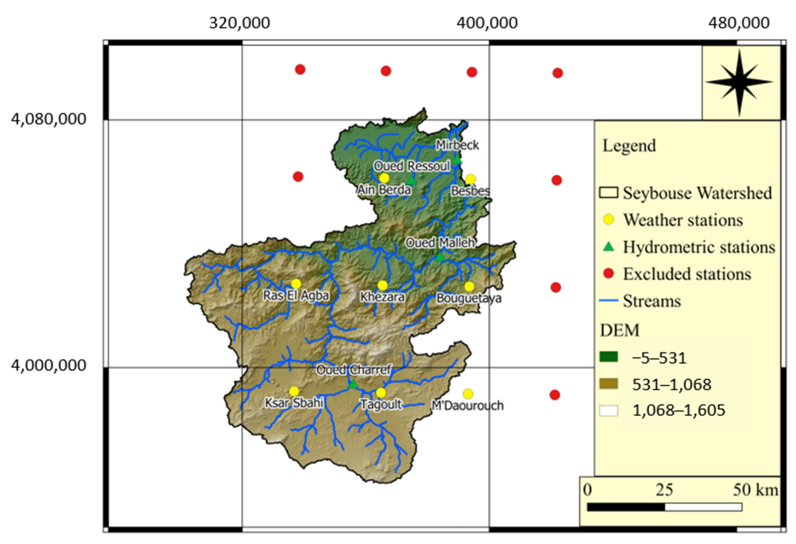
The study area is the semi-arid Seybouse basin located in the northeastern part of Algeria. It covers 6775 km². The elevation in the basin ranges from 0 to 1600 m.a.s.l. (Figure 1).

It is bounded in the North by the Mediterranean Sea, to the East and West by the Constantinois coastline, and to the South by the Kébir-Rhumel, Constantinois and Medjerda high plateaus. The Seybouse river recharges to the Mediterranean Sea at Sidi Salem towards the South of the city of Annaba. The Seybouse basin rises in the semi-arid high plains on the southern slope of the Atlas Tellien, flowing from South to North. According to the Natural Waer Resource Agency, the Seybouse basin is divided into five sub-basins [12]. However, in this study, the basin is divided into 62 sub basins to better represent and model the real-world hydrological processes.

2.1.1. Hydro-Climatology

The upper Seybouse is a mountainous area with a typically Mediterranean climate, with hot summers and relatively mild winters; the annual amplitude characterizes the degree of continental climate in the southern part of the Seybouse basin. In the middle of Seybouse, the hot season runs from May to October, with an average temperature of 25 °C, peaking in August, and corresponding to the dry season, with an absence of precipitation. The wet season runs from October to April, with average temperatures below 15 °C. The maximum temperature recorded in the lower Seybouse is around 46 °C and the minimum is around 23 °C [13]. The mean annual temperature in the entire basin is recorded as approximately 20 °C.

The spatial distribution of rainfall fields in the region is subject to three influences; that of altitude, topographical conditions of longitude and finally that of distance from the sea. The rainfall intensity increases with altitude and from West to East but is higher on slopes exposed to wet winds than on leeward slopes. It decreases moving away from the coast [13]. The mean annual rainfall in the entire basin varies from 500 mm to 1100 mm approximately which proves a heterogenous rainfall distribution in the study area.

2.1.2. Hydrology and Hydrogeology

The Seybouse basin is characterized by a heterogeneous, compartmentalized relief (plains, mountains, valleys, hills, slopes, etc.). The basin drains a series of highly heterogeneous regions. The high plains, with their simple relief and low or even non-existent runoff, are followed by the rugged Atlas Tellien, with its highly complex structure. The wadis have irregular flows. The longitudinal profile allows rapid drainage. The Seybouse basin has a hydrographic network of over 3000 km, with forty-two wadis over 10 km long. It is made up of highly heterogeneous natural units, e.g., mountains, depressions, and plateaus resulting in different modes of feeding and runoff. The existence of depressions containing alluvial aquifers through which the Seybouse flows regulates the seasonal flow and results in low to zero river flows in summer despite the high proportion of winter rainfall received by this mountain range.

2.1.3. Database

The Seybouse basin contains 17 rain gauges, and 4 hydrometric stations. However, the database has data gap issues in different scales (i.e., monthly, or annually). For instance, the hydrometric station that is closest to the basin outlet, chosen as the station to calibrate the model with, has discharge data available from 1968 to 1991. Rain gauges have rainfall data in different measurement time steps (annual mean, monthly mean or daily and daily or monthly maximum). Due to the rainfall measurements possessing significant data gaps, Climate Forecast System Reanalysis (CFSR) of The National Centers for Environmental Prediction (NCEP) weather estimates are used. The CFRS system includes daily precipitation, wind, relative humidity, and solar radiation data from 1979 to 2014. The CFSR was designed and executed as a global, high resolution, coupled atmosphere-ocean-land surface-sea ice system to provide the best estimate of the state of these coupled domains over this period. In situ rain gauge data and CFRS data showed good correlations for the periods where both databases had available data. Therefore, databases were used for model calibration and validation for the period of 1979–1991. Calibration and validation periods were divided into two parts after excluding two years of warming up (training period) to avoid initial condition-related uncertainty issues.

2.2. SWAT Modelling

The Soil and Water Assessment Tool (SWAT) is a semi-distributed, continuous-time, process-based, physical hydrological model. It is meant to assess the impacts of water resource management alternatives in large river basins [14]. The spatial distribution of model parameters is controlled by subbasins having distinct spatial positions and hydrological response units (HRUs) which are lumped within subbasins with respect to distinct combinations of land use, soil, and slope characteristics. The SWAT model requires a wide range of parameters using manual or automated calibration processes such as shuffled complex evolution method SCE-UA [15,16,17], semi-automated SUFI-2 method providing sensitivity and uncertainty analysis [18,19,20] and GLUE [21,22]. SUFI-2 conducts a comprehensive optimization and uncertainty analysis via employing a global search approach, enabling it to handle a considerable quantity of parameters.

SWAT embedded in geographic information system platforms, e.g., QGis and ArcGis, works via a graphical user interface and allows users to design hydrological models. Model design is supported by digital elevation topographical map (DEM), river networks, land use, soil, and slope maps in order first to create subbasins and then hydrological units.

2.2.1. Model Inputs

The basic data set required for a SWAT model includes: a DEM of the basin, climate data, land use/land cover and soil data. The DEM used for this study was of 30 m resolution from NASA’s Shuttle Radar Topography Mission (SRTM). The soil map is obtained from FAO and related soil textures and soil hydraulic groups are written in SWAT database (

Table 1. Soil classes in the basin with associated soil textures and hydraulic groups.

Soil Group Numbers	Soil Textures	Hydraulic Group
1	CLAY	D
2	CLAY	C
3	CLAY_LOAM	D
4	LOAM	D
5	LOAM	D
6	SANDY_CLAY_LOAM	C
7	LOAM	D

).

Climate data include daily precipitation, temperature, solar radiation, relative humidity, and wind data from the CFRS dataset which is compatible with SWAT. Eight weather stations from the CFRS system were considered as weather data out of sixteen stations. Discharge data from 4 hydrometric stations is used during calibration for rainfall-runoff modelling (Figure 1).

The land use data is obtained from ESA’s Global land use GlobCover, 2009 data (

Table 2. Global Land Use GlobCover with related SWAT land use classes.

GlobCover Code	GlobCover Definition	SWAT Code	SWAT Definition
AGIR	Post-flooding or irrigated crops	AGRL	Agricultural land
AGRF	Rainfed croplands	AGRL	Agricultural land
AGMX	Cropland (50–70%)/grassland, shrubland, forest (20–50%)	AGRL	Agricultural land
CRGR	Grassland, shrubland, forest) (50–70%)/cropland (20–50%)	CRGR	Cropland/grassland
FRSE	Broadleaved evergreen	FRST	Forest-evergreen
FRSD	Broadleaved deciduous forest	FRSD	Forest-deciduous
PINE	Needle-leaved evergreen forest	PINE	Pine
FRST	Mixed broadleaved and needle-leaved forest	FRST	Forest-mixed
RNG1	Mosaic forest or shrubland (50–70%)/grassland (20–50%)	RNGB	Range-brush
RNE1	Mosaic grassland (50–70%)/forest or shrubland (20–50%)	RNGE	Range-grasses
FRST	Closed to open (>15%) evergreen or deciduous, shrubland (<5 m)	FRST	Forest-mixed
RNGB	Sparse (<15%) vegetation	RNGB	Range-brush
URBN	Artificial surfaces and associated areas (urban areas >50%)	URMD	Residential
BSVG	Bare areas	BSVG	Barren or sparsely vegetated
WATB	Water bodies	WATR	Water bodies

). Global land use GlobCover data is adapted to the SWAT codes and a new land use database is created to be read by SWAT model easily.

2.2.2. Model Design

The hydrologic cycle in the SWAT model is based on the water balance equation:

$$\mathrm{S}{\mathrm{W}}_{\mathrm{t}}=\mathrm{S}{\mathrm{W}}_0+{\sum }_{i=1}^t({\mathrm{R}}_{\mathrm{d}\mathrm{a}\mathrm{y}}-{\mathrm{Q}}_{\mathrm{s}\mathrm{u}\mathrm{r}\mathrm{f}}-{\mathrm{W}}_{\mathrm{s}\mathrm{e}\mathrm{e}\mathrm{p}}-{\mathrm{E}}_{\mathrm{a}}-{\mathrm{Q}}_{\mathrm{g}\mathrm{w}})$$

(1)

where $\mathrm{S}{\mathrm{W}}_{\mathrm{t}}$ is the humidity of the soil (mm), $\mathrm{S}{\mathrm{W}}_0$ is the base humidity of the soil (mm), $t$ is time (days), ${\mathrm{R}}_{\mathrm{d}\mathrm{a}\mathrm{y}}$ is rainfall volume (mm), ${\mathrm{Q}}_{\mathrm{s}\mathrm{u}\mathrm{r}\mathrm{f}}$ is the value of surface runoff, ${\mathrm{W}}_{\mathrm{s}\mathrm{e}\mathrm{e}\mathrm{p}}$ is the value of seepage of water from the soil into deeper layers, ${\mathrm{E}}_{\mathrm{a}}$ is the value of evapotranspiration (mm), and ${\mathrm{Q}}_{\mathrm{g}\mathrm{w}}$ is the value of underground runoff (mm).

Subbasin and stream calculations are performed with the automatic delineation tool incorporated in QSWAT 3 version 1.6.3. Land use map, soil classification map and slope map are created for the Seybouse basin and introduced to the database concerning the global land use and user soil options in the QSWAT 3 1.6.3.

2.2.3. Hydrologic Response Unit (HRU)

HRUs are specified subunits within each subbasin. They are lumped land areas with overlapping unique combination of land use, soil, and slope classes. Each subbasin contains at least one HRU and one main tributary.

HRUs are created using physically based data, i.e., land use data, soil type and soil properties and digital elevation model for slope calculation (Figure 2, Figure 3 and Figure 4). HRUs are created by splitting individual subbasins apart, resulting in distinct combinations of land use, slope, and soil classes within each subbasin that can represent a different number of HRUs. These HRUs, found across subbasins, share comprehensive attributes like soil type, land use, and slope. Calculations related to physical processes performed separately on these HRUs are aggregated by summation through the outlet point for each corresponding subbasin. While creating the HRUs, a threshold is used by defining the land use, soil, and slope classes percentage in a subbasin. The first threshold is applied to land uses by its percentage in a subbasin area that eliminates small land covers in each subbasin. Secondly, a percentage of soil classes relative to land use area after first threshold eliminates the unimportant (in size) soil occupations. The final threshold is the elimination of slope classes relative to the soil area by another percentage to eliminate minor slope classes [23]. The threshold information can be addressed in

Table 3. Threshold definitions for land use, soil and slope classes used in formation of HRUs.

HRU Threshold	Minimum % of Land Area
Land use by subbasin area	0
Soil class by land use area after 1st threshold	10
Slope class by soil class area after 2nd threshold	15

.

2.2.4. Swat Model Simulations

The main objective of the simulations is to calibrate and validate the model with respect to existing discharge observations from ground stations to finally obtain a value of groundwater recharge from the validated model. Therefore, meteorological data was used as input and the only output variable was the river discharge. SWAT provides two methods for surface runoff estimation: the Soil Conservation Service (SCS) curve number and the Green-Ampt infiltration method. In the present study, the SCS curve number method is preferred. The SCS method uses the following formula for runoff computation to estimate runoff under varying land use and soil types [24]:

$$Q_{surf}=\frac{{{(R}_{day}-I_a)}^2}{\left(R_{day}-I_a+S\right)}$$

(2)

$$S=25.4(\frac{1000}{CN}-10)$$

(3)

where $Q_{surf}$ is accumulated runoff (mm), $R_{day}$ is daily rainfall depth, $I_a$ is the initial abstractions (mm), $S$ is the retention parameter (mm) and $CN$ is the curve number.

After model simulation, the model is checked via SWAT Error Checker for possible inconveniences in hydrological cycle prior to calibration period. Model calibration can accomodate these inconveniences, if any.

For instance, surface runoff is found to be too low during the pre-calibration period to be used as an index in the calibration period. This could be due to high evaporation and transpiration present in the region or underestimation of surface runoff during simulation. In any case, it seems that model design is meaningful, and calibration can be functional at this point.

2.2.5. Calibration, Sensitivity, and Validation

Hydrological models face different levels of inaccuracies coming from different sources of uncertainty. Major uncertainty sources are input forcings, model parameters, and model structure. Processes-based distributed hydrological models provide a large variety of parameters so that models can better represent the real-world hydrological systems. However, it is known that the more parameters a model is run with, the more uncertainty its simulations would possess. Therefore, rigorous calibration, validation, and uncertainty and sensitivity analyses steps are required.

The SWAT Calibration and Uncertainty Program (SWAT-CUP), a computer-based software is widely used for calibration, validation, and sensitivity analysis purposes for SWAT models [25]. The program provides uncertainty and sensitivity analyses for multi-site calibration through different calibration algorithms such as the Sequential Uncertainty Fitting version-2 (SUFI-2), Particle Swarm Optimization (PSO), Generalized Likelihood Uncertainty Estimation (GLUE), Parameter Solution (ParaSol), Markov Chain Monte Carlo (MCMC), that can be used for analyzing SWAT outputs based on different cost functions. In this study, the SUFI-2 algorithm is used to calibrate the SWAT model. The calibration algorithm, SUFI-2 is an iterative algorithm and projects all the model uncertainties to a certain parameter range. The total uncertainty is determined by the 95% predictive uncertainty (95PPU) calculated at the 2.5% and 97.5% levels of the cumulative distribution of an output variable which disallows 5% of very inaccurate simulations. SUFI-2 assumes, at first, a large parameter uncertainty. Therefore, the measured data initially falls within the 95PPU. Then, the model decreases this uncertainty step by step while monitoring the p-factor and the r-factor. In each step, previous parameter ranges are updated by calculating the sensitivity matrix (i.e., Jacobian matrix), and equivalent of a Hessian matrix, which is then followed by the covariance matrix calculation, 95% confidence intervals, and correlation matrix. Parameters are later updated in such a way that the new ranges are always smaller than the previous ranges and are centered on the best simulation.

Hydrological modelling of a basin does not occur in a unique way. It is always possible to calibrate a model with different parameter sets which is explained by the equifinality phenomenon in hydrology [26,27]. Therefore, acknowledging which parameters really represent and affect the physical processes in a basin is essential. This can be done through sensitivity analysis. Sensitivity analysis is the process of determining the change in model output based on the changes in parameters space. Global sensitivity analysis is where the uncertainty in outputs to the uncertainty in each input factor is examined over their entire range of interest. It is considered to be global when all the input variables are modified simultaneously [28]. A multiple regression analysis called the t-test is used for sensitivity analysis in the SUFI-2 algorithm. T-stat is the ratio of the coefficient of a parameter to its standard error. If the coefficient is higher than its standard error, then the parameter is likely to be sensitive [29]. The p-value in t-tests is more decisive to understand if the parameter is sensitive. A low p-value (<0.05) generally indicates the model response changes related to the changes in parameter. A large p-value is associated with non-sensitive parameters.

The SUFI-2 algorithm provides two statistical terms to quantify the fitness between the observation and the simulation, which is expressed as 95PPU. These are called p-factor and r-factor. p-factor is the percentage of the measured data covered by the 95 PPU simulation results while r-factor is the width of the cover. The aim is to cover the maximum of the observed data in 95PPU and decrease the width of the 95PPU band. In general, >70% of p-factor and r-factor around 1 is considered as a good threshold for discharge data [18,19].

Validation data should be completely different from the calibration data for a rigorous and robust hydrological modelling practice. Therefore, data from four discharge observation stations were divided into two parts for the calibration and validation steps. All the stations are used for both calibration and validation steps with respect to different time periods (

Table 4. Names and locations of the discharge observation stations used for model calibration and validation.

Discharge Observation Station	UTM Easting	UTM Northing
Mirbeck	389,563.39	4,066,965.44
Oued Ressoul	374,818.87	4,060,178.06
Oued Malleh	383,958.91	4,035,417.7
Oued Charref	355,941.82	3,994,372.54

).

In this way, the model is validated, with the parameter set decided during the calibration, with data from different periods which are unknown to the model, i.e., as we would have to do in a prediction case.

2.2.6. Cost Functions

• Nash—Sutcliffe (NS); is one of the most preferred evaluation criteria in literature. It takes its maximum value (i.e., 1) when the ratio of the error variance of model estimation to the variance of observed time series is zero [30].

  $$NS=1-\frac{\sum _{k=1}^{k=n}{\left(s\left(k\right)-q\left(k\right)\right)}^2}{\sum _{k=1}^{k=n}{\left(q\left(k\right)-\overline{q}\right)}^2}$$

  (4)

  where $s\left(k\right)$ is estimated output, $q\left(k\right)$ is observed output, $\overline{q}$ is mean observed output, $n$ is total number of time steps of variables, and $k$ is discrete time.
• Coefficient of determination (${\mathrm{R}}^2$); is defined as the proportion of the variation in the dependent variable that is modelled from the independent variables. It measures how well the simulated variable represents the observed variable.

  $${\mathrm{R}}^2=\frac{\sum _{k=1}^{k=n}{\left(\left(q\left(k\right)-\overline{q}\right)\left(s\left(k\right)-\overline{s}\right)\right)}^2}{\sum _{k=1}^{k=n}{{\left(\left(q\left(k\right)-\overline{q}\right)\right)}^2\sum _{k=1}^{k=n}\left(\left(s\left(k\right)-\overline{s}\right)\right)}^2}$$

  (5)

  where $s\left(k\right)$ is estimated output, $q\left(k\right)$ is observed output, $\overline{q}$ is mean observed output, $\overline{s}$ is mean simulated output, $n$ is total number of time steps of variables, and $k$ is discrete time.
• Percentage bias ($PBIAS$); is a measure of the difference between the amount of produced water by the basin and the amount of estimated water by the model. This criterion considers water volume transfers explicitly. A lower value indicates a better simulation. Positive values indicate that the model underestimates the observations while negative values indicate the inverse.

  $$PBIAS=\frac{\sum _{k=1}^{k=n}\left(q\left(k\right)-s\left(k\right)\right)}{\sum _{k=1}^{k=n}q\left(k\right)}$$

  (6)

  where $s\left(k\right)$ is estimated output, $q\left(k\right)$ is observed output, $\overline{q}$ is mean observed output, $\overline{s}$ is mean simulated output, $n$ total number of time steps of variables, and $k$ is discrete time.
• Kling–Gupta efficiency criteria ($KGE)$; is a measure of the linear regression coefficient between observed and simulated variables.

  $$KGE=1-\sqrt{{\left(r-1\right)}^2+{\left(a-1\right)}^2+{\left(\beta -1\right)}^2}$$

  (7)

  where $a=\frac{{\sigma }_s}{{\sigma }_q}$, and $\beta =\frac{{\mu }_s}{{\mu }_q}$ and $r$ is the linear regression coefficient between observed and simulated variables, ${\sigma }_s$ and ${\sigma }_q$ are standard deviation, and ${\mu }_s$ and ${\mu }_q$ are means of simulated and observed variables [31].

3. Results

3.1. Calibration and Validation Results

The SWAT model is calibrated with the database concerning the years between 1979 and 1986. The first two years are used for model training. Therefore, calibration results cover the years from 1981 to 1986. Validation period was between 1987 and 1991. Two years of training were also adapted for validation as in calibration but for the period between 1985 and 1986. Calibration with the SUFI-2 algorithm is an iterative approach. Each calibration run is composed of 1000 iterations. The more parameters that the model is calibrated with, the more iterations the model would require. In the case of the present study, 1000 iterations were needed to obtain a global sensitivity analysis. A global sensitivity analysis is performed following a run in SWAT-CUP model to understand the relative influence of the change in all parameters on the change of model output.

Sensitivity analysis results present the least and most sensitive parameters to the changes applied to the model parameters. Global sensitivity analysis and evaluation are repeated several times, since after each run sensitivity analysis could give different results. Final sensitivity analysis results of model parameters are given (

Table 5. Sensitivity analysis results.

Parameter Name	t−Stat	p-Value
r__SOL_K(2).sol__C	−0.08	0.93
v__SURLAG.bsn	0.10	0.92
v__SOL_ALB(1).sol__C	−0.17	0.85
v__SOL_ALB(1).sol__D	0.19	0.85
v__REVAPMN.gw	−0.21	0.83
v__CH_K2.rte	−0.26	0.79
v__EPCO.hru	0.24	0.81
r__SOL_AWC(2).sol__D	0.41	0.68
v__CH_N2.sub	0.43	0.67
v__ALPHA__BF.gw	0.43	0.67
r__PLAPS.sub	−0.60	0.55
v__GW_REVAP.gw	−0.63	0.53
v__SOL_BD().sol__C	0.67	0.66
r__SOL_K(2).sol__D	−0.71	0.48
v__ALPHA_BNK.rte	0.63	0.53
r__SOL_AWC(2).sol__C	1.2	0.23
r__OV_N__.hru	−1.23	0.22
r__SOL_AWC(1).sol__C	−1.32	0.18
v__ESCO.hru	1.56	0.12
v__CH_N1.sub	−1.65	0.098
v__GWQMN.gw	−1.85	0.065
v__ GW_DELAY.gw	−1.88	0.06
r__SOL_AWC(1).sol__D	1.97	0.05
r__SOL_K(1).sol__D	−2.2	0.02
r__SOL_K(1).sol__C	2.6	0.009
v__CH_K1.sub	4.97	0.000001
v__SOL_BD().sol__D	−7.04	0
v__RCHRG_DP.gw	−9.9	0
r__CN2.mgt	−42.7	0

). The six most sensitive parameters were the ones with p-value equal to or lower than 0.05.

These parameters are SCS curve number (CN2.mgt) deep aquifer percolation fraction (RCHRG_DP.gw), soil bulk density for soil hydraulic group D (SOL_BD__D), effective hydraulic conductivity in tributary channel alluvium (CH_K1.sub), saturated hydraulic conductivity of the first soil layer for soil hydraulic group C (SOL_K(1)__C), and saturated hydraulic conductivity of the first soil layer for soil hydraulic group D (SOL_K(1)__D). Although there were parameters with low sensitivity for each iteration, the model is still calibrated with these parameters not to exclude the minor effects on the calibration and the validation.

Some of the parameters are calibrated with respect to certain soil layers, indicated as (1) for first soil layer and (2) for second soil layer; or soil hydraulic groups, indicated as “__D” for soil hydraulic group D and “__C” for soil hydraulic group C, to better represent the spatial variability of these parameters. Other parameters, e.g., groundwater parameters, are run for whole HRUs. Different groundwater, soil and surface related parameters are used in calibration periods following the sensitivity analysis. The calibrated parameters are presented in

Table 6. Final limit ranges and the fitted parameter values of the calibrated model.

Name	Definition	Min	Max	Fit
v__SOL_ALB(1).sol__D	Moist soil albedo of the first soil layer	0	0.4	0.01
v__SOL_ALB(1).sol__C	Moist soil albedo of the first soil layer	0	0.4	0.01
v__GWQMN.gw	Threshold water depth in the shallow aquifer for return flow (mm H2O)	0	5700	5020
v__GW_REVAP.gw	Groundwater “revap” coefficient	0.01	0.5	0.24
v__GW_DELAY.gw	Groundwater delay time (days)	0	100	92
v__REVAPMN.gw	Threshold water depth of shallow aquifer for “Revap” or percolation (mm H2O/)	300	400	343
v__ESCO.bsn	Soil evaporation compensation factor	0.1	1	1
v__EPCO.bsn	Plant uptake compensation factor	0.1	1	0.86
r__SOL_AWC(1).sol__D	Available water capacity (mm H2O/mm)	0	8	1.55
r__SOL_AWC(2).sol__D	Available water capacity (mm H2O/mm)	0	8	1.03
r__SOL_AWC(1).sol__C	Available water capacity (mm H2O/mm)	0	8	1.6
r__SOL_AWC(2).sol__C	Available water capacity (mm H2O/mm)	0	8	4.5
r__SOL_K(1).sol__D	Saturated hydraulic conductivity (mm/h)	0.1	2000	0.001
r__SOL_K(2).sol__D	Saturated hydraulic conductivity (mm/h)	0.1	2000	5.9
r__SOL_K(1).sol__C	Saturated hydraulic conductivity (mm/h)	0.1	2000	0.6
r__SOL_K(2).sol__C	Saturated hydraulic conductivity (mm/h)	0.1	2000	8.1
r__OV_N.hru	Manning’s “n” value for overland flow	−0.3	0.3	−0.03
r__CN2.mgt	Initial SCS runoff curve number	−0.99	0.99	−0.94
v__ALPHA_BF.gw	Baseflow alpha factor (days)	0	0.1	0.08
v__ALPHA_BNK.rte	Baseflow alpha factor for bank storage (days)	0	1	0.92
v__SURLAG.bsn	Surface runoff lag coefficient	0.05	24	7.8
v__CH_K1.sub	Effective hydraulic conductivity in tributary channel alluvium (mm/h)	0	500	183
v__CH_K2.rte	Effective hydraulic conductivity in main channel alluvium (mm/h)	0	500	339
v__CH_N1.sub	Manning’s “n” value for the tributary channels	0.1	10	1.6
v__CH_N2.rte	Manning’s “n” value for the main channel	0.1	10	0.05
v__RCHRG_DP.gw	Deep aquifer percolation fraction	0	1	0.001
v__SOL_BD.sol__C	Moist bulk density (mg/m3 or g/cm3)	0.8	2.5	2.2
v__SOL_BD.sol__D	Moist bulk density (mg/m3 or g/cm3)	0.8	2.5	0.81
r__PLAPS.sub	Precipitation lapse rate (mm H2O/km)	−1000	1000	−0.05

.

Model calibration is performed with two iterative approaches: by replacing the parameter calibration ranges directly (indicated with v__parameter.name) and multiplying the ranges with new range +1 (indicated by r__parameter.name). The latter is usually suggested for the parameters where the spatial distribution of the parameter is important, and calibration should be done considering spatial variations in the basin. For instance, groundwater parameters are replaced with new ranges at each iteration (i.e., v__parameter.name.gw) such as groundwater evaporation factor, v_GW_REVAP.gw, and deep aquifer percolation fraction, v__RCHRG_DP.gw, while surface runoff parameter ranges are multiplied with “new ranges +1” such as r__CN2.mgt and r__OV_N.hru (Table 6).

Some of the parameters are calibrated with respect to certain soil layers, indicated as (1) for first soil layer and (2) for second soil layer; or soil hydraulic groups, indicated as “__D” for soil hydraulic group D and “__C” for soil hydraulic group C, to represent better the spatial variability of these parameters. Other parameters, e.g., groundwater parameters, are run for whole HRUs. Different underground, soil and surface related parameters are calibrated following the sensitivity analysis (Table 6).

It is important to note that for a rigorous result evaluation, one should consider using the calibrated parameter ranges rather than the final fit. The range indicates the uncertainty levels on those variable estimations by giving an envelope of possible values of the parameter. On the other hand, fitted parameter lacks the uncertainty information related to that parameter.

3.2. Model Performance Evaluation

Model calibration and validation results are evaluated graphically and statistically as explained in Section 2.2.6. For the calibration period, the model successfully managed to reproduce overall discharge trends and simulated the flood peaks well, especially for the Mirbeck station (Figure 5).

Simulation results are relatively less efficient at the Malleh and Ressoul stations with more underestimation of the main flood event recorded in 1984 winter (Figure 6 and Figure 7). However, the model perfectly reproduced most of the other discharge anomalies. However, for the most upstream station, (i.e., Charref) the model performed good simulations with an underestimation for only one flood episode (Figure 8).

We can observe that the model underestimates the flood peaks more in the validation period than in the calibration period (Figure 9, Figure 10, Figure 11 and Figure 12). However, the model generally performs reliable simulations for the validation period.

The statistical results of model calibration and validation are given in

Table 7. Statistical results of the model calibration and validation for four discharge stations.

	Calibration				Validation
Station	R2	NS	PBIAS	KGE	R2	NS	PBIAS	KGE
Mirbeck	0.7	0.7	20	0.7	0.6	0.6	30.7	0.6
Ressoul	0.6	0.5	37	0.3	0.8	0.4	53.5	0.15
Malleh	0.7	0.6	12	0.6	0.6	0.6	5.0	0.6
Charref	0.6	0.5	8	0.8	0.03	−0.12	17.3	0.07

for four hydrometric stations. The results showed reliable results overall varying mostly from satisfactory to very good results for the calibration according to

Table 8. Evaluation ranges for calibration and validation results.

Criteria	Very Good	Good	Satisfactory	Unsatisfactory
R2	0.75 ≤ R2 ≤ 1	0.65 ≤ R2 < 0.75	0.50 ≤ R2 < 0.65	R2 < 0.5
NS	0.75 ≤ NS ≤ 1	0.65 ≤ NS < 0.75	0.50 ≤ NS < 0.65	NS < 0.5
KGE	0.9 ≤ KGE < 1	0.75 ≤ KGE < 0.9	0.5 ≤ KGE < 0.65	KGE < 0.5
PBIAS	$\left|\mathrm{PBIAS}\right|$ < 10	$10 \le \left|\mathrm{P}\mathrm{B}\mathrm{I}\mathrm{A}\mathrm{S}\right|$ < 15	$15 \le \left|\mathrm{P}\mathrm{B}\mathrm{I}\mathrm{A}\mathrm{S}\right|$ < 25	$25 \le \left|\mathrm{P}\mathrm{B}\mathrm{I}\mathrm{A}\mathrm{S}\right|$

[32,33]. For the validation period, there were less satisfactory results at several stations.

The model simulated discharges with satisfactory to good statistical results at Mirbeck station both for calibration and validation. That is an indicator for good representation of water balance in the watershed during low or high flows. Only the PBIAS score degraded significantly and showed unsatisfactory results for validation. Calibration results obtained at the other stations (e.g., Malleh, Ressoul, and Charref) are also reliable for the rest of the watershed apart from relatively lower performance at the Ressoul station with unsatisfactory scores for KGE and PBIAS (Table 7). Both calibration and validation scores were satisfactory for Malleh stations and likewise for Mirbeck. However, it can be noted that simulation performances decreased for the validation period for Ressoul and Charref stations. For Ressoul station, the performance scores were unsatisfactory except for R². For Charref station, the performance scores were unsatisfactory except PBIAS.

Once the model calibration and validation are performed, the SWAT model is rerun for the whole period with the calibrated parameters to calculate the amount of total aquifer recharge and deep aquifer recharge. The results show that annual average total and deep aquifer recharge values are 345 mm and 38 mm. Re-evaporation from shallow aquifer by the soil and plants is 292.3 mm while aquifer discharge to the river through return flow is 37 mm annually (

Table 9. Water balance results with the validated model.

Basin Values	Annual Averages (mm)
Precipitation	1037.1
Snowfall	6.61
Snowmelt	6.59
Surface runoff	9.21
Lateral soil flow	74.2
Groundwater discharge	36.7
Percolation out of soil	347.7
Total aquifer recharge	345
Deep aquifer recharge	38
Re-evaporation	392.3
Evapotranspiration	627

). Net annual average infiltration is approximately 150 mm which is equivalent to 15% of the net annual average rainfall. Whereas the evapotranspiration is 61% and the river flow is 12% of the net annual average, which is consistent with the findings of other studies in the same basin [13,34,35].

The results demonstrated that a modest amount of rainfall becomes surface runoff. Moreover, the groundwaters feed the rivers only with an amount equal to 3.5% of annual rainfall. On the other hand, evapotranspiration and re-evapotranspiration from shallow aquifers is quite dominant in the water budget of the watershed. Moreover, only 38 mm of water infiltrates deeper aquifers.

4. Discussion

Calibrating the model with discharge data obtained from four hydrometric stations corresponding to four sub basins was a challenging task (i.e., subbasins 2, 8, 51, and 60). Since the different hydrological responses are created at different stations, the model had to reproduce different discharge regimes with the same rainfall data recorded in physical stations in different parts of such a vast watershed. For instance, high flows and low flows were observed in different downstream tributaries (e.g., Mirbeck and Oued Ressoul, respectively) during the same period of the year.

Statistically speaking, performance evaluation scores were accumulated mostly in the reliable limits, varying from satisfactory to good results. Even though the model validation performance is less than that of calibration, the deviation was affordable. Considering that the model is calibrated with some of the most extreme events recorded in the region, model validation performance was acceptable in simulating mostly moderate to low flows with fewer significant high flow episodes.

Simulated hydrographs showed that the calibrated model could reproduce the observed discharge trends. This is the case for most of the low flows and peaks. Moreover, average volume bias error remained at satisfactory levels. This is an important indicator for process-based semi distributed models for satisfactory calibration especially when the model is calibrated and validated for multiple hydrometric stations in the same watershed.

Model calibration for Mirbeck station was more crucial since it is the closest station to the basin outlet. The best calibration results are obtained at this station which shows that the model could represent the hydrological cycle in the watershed and reproduce the discharge observed in the main channel despite the existence of extreme events.

Simulations were performed using estimated long-term rainfalls from a weather forecast system and observed in-situ discharge data. When the simulation accuracies in calibration and validation steps are considered, it is a significant output that model was capable of reproducing observed output data with estimated input data for four stations at once. Moreover, observed rainfalls in the basin showed good correlation with estimated ones, confirming that CFRS estimated rainfalls can represent the real rainfall fields well in the Seybouse basin. This can be an insight for future studies to use rainfall estimates for hydrological or hydrogeological studies. Moreover, the model is calibrated and validated with discharge data covering the period between 1979 and 1991. Unfortunately, there was no available discharge data beyond 1991. Other studies also mentioned the data unavailability and used periods of data for model calibration for different stations [36]. In this work, on the other hand, the model is calibrated with the same period of data for all stations.

Several studies suggested increase and shifts in average annual rainfalls after the 90s and drought conditions focused only on the central part of the basin [37]. Even though the data used in this study do not cover recent warmer decades with relatively higher evaporation losses [36,38], the process-based model based on rigorous calibration and validation practices is considered capable of performing accurate simulations also with more recent data. The model’s relatively good performance over the 1979–1991 period provides the basis for a new data collection campaign to test the model against climatic conditions impacted by global warming in more recent years.

Proposing a reliable water balance model would allow future works to compute river discharge or groundwater recharge to feed groundwater hydrodynamic models for water resource management alternatives for nearby residences, agricultural lands, and industry. Water balance calculations obtained by the calibrated model shows consistent results. Water balance, annual rainfall and evapotranspiration values correspond to the values found in the literature [34,35]. Moreover, estimated water uptake from shallow aquifers and percolation to deeper aquifer present reasonable amounts. Therefore, the estimated water amount infiltrating into the aquifers can be used to feed the hydrodynamic model to assess the groundwater fluctuations as mentioned earlier as an objective of the project.

5. Conclusions

This work presents an example of hydrological modelling practices with an open-source tool, i.e., SWAT, in a semi-arid southern Mediterranean, Seybouse, basin. Seybouse basin is marked with inaccurate and scarce hydro-meteorological data. Despite the data availability issues, water scarcity underscores the importance of water resource management applications and rigorous hydrological modelling practices. The objective of this study is to calibrate the model with different hydrometric stations to simulate different discharge trends in different locations of the basin to eventually obtain groundwater recharge estimation. The estimated groundwater recharge is an important result to feed future groundwater models as an input variable to apply groundwater resource management scenarios.

To provide a rigorously calibrated and validated hydrological model, estimated long-term rainfall data, considering the data unavailability, are used to calibrate observed discharge data for four hydrometric stations in SWAT model. Provided hydrographs and statistical results showed that the model could produce reliable simulations for all the hydrometric stations. Model calibration results show that model could simulate discharge with NS ≥ 0.5, R² ≥ 0.6, KGE ≥ 0.6 in average and PBIAS < 37 which represent overall satisfactory to good results. Although the validation results are relatively less accurate, they still represent satisfactory results for at least two out of four stations (Table 8 and Table 9). Therefore, model calibration and validation results are overall satisfactory to assure water budget calculation accuracy which provides estimated groundwater recharge. This could be used to feed a hydrodynamic model of the basin which will be the next step in this project.

Data unavailability issues and the model’s relatively good performance suggest that further data acquisition campaigns would be necessary to test model simulation accuracy under the ongoing global warming changes. Further applications could include performing hydrological simulations with different hydrological model types such as statistic-based hydrological models e.g., neural networks, to compare with the process-based hydrological models.

References

- Morante-Carballo, F.; Montalván-Burbano, N.; Quiñonez-Barzola, X.; Jaya-Montalvo, M.; Carrión-Mero, P. What Do We Know about Water Scarcity in Semi-Arid Zones? A Global Analysis and Research Trends. Water 2022, 14, 2685. [Google Scholar] [CrossRef]
- Lu, Y.; Liu, Y.; Huang, J.; Yang, X.; Yin, H. Numerical modeling of groundwater recharge in a coastal city with multi-layered aquifer systems. Water Sci. Eng. 2019, 12, 293–301. [Google Scholar] [CrossRef]
- Dillon, P.; Pavelic, P.; Page, D.; Vanderzalm, J.L.; Pavelic, V. Global overview of managed aquifer recharge: Regional applications, success stories, and future prospects. Hydrogeol. J. 2018, 26, 395–420. [Google Scholar]
- Aladenola, O.O.; Durowoju, O.S.; Adedeji, O.H. Potential impacts of rainwater harvesting on groundwater recharge in a typical basement complex region. J. Afr. Earth Sci. 2016, 114, 53–60. [Google Scholar] [CrossRef]
- Elliott, D.; Singh, R.; Dillon, P. Performance evaluation of permeable reactive barriers for groundwater recharge. J. Hydrol. 2016, 538, 842–853. [Google Scholar] [CrossRef]
- Kurtulus, B.; Yaylım, T.N.; Avşar, O.; Kulac, H.F.; Razack, M. The Well Efficiency Criteria Revisited—Development of a General Well Efficiency Criteria (GWEC) Based on Rorabaugh’s Model. Water 2019, 11, 1784. [Google Scholar] [CrossRef]
- Kilic, D.; Rivière, A.; Gallois, N.; Ducharne, A.; Wang, S.; Peylin, P.; Flipo, N. Assessing water and energy fluxes in a regional hydrosystem: Case study of the Seine basin. Comptes Rendus. Géosci. 2023, 355, 1–21. [Google Scholar] [CrossRef]
- Chow, V.T.; Maidment, D.R.; Mays, L.W. Applied Hydrology; McGraw-Hill: New York, NY, USA, 1988. [Google Scholar]
- Beven, K.J. Rainfall-Runoff Modelling: The Primer; John Wiley & Sons: Hoboken, NJ, USA, 2011. [Google Scholar]
- Jajarmizadeh, M.; Harun, S.; Salarpour, M. A review on theoretical consideration and types of models in hydrology. J. Environ. Sci. Technol. 2012, 5, 249–261. [Google Scholar] [CrossRef]
- Devi, G.K.; Ganasri, B.P.; Dwarakish, G.S. A review on hydrological models. Aquat. Procedia 2015, 4, 1001–1007. [Google Scholar] [CrossRef]
- Louamri, A. Le bassin-versant de la Seybouse (Algérie orientale): Hydrologie et aménagement des eaux. Constantine 2013, 1, 315. [Google Scholar]
- Hebal, A. Analyse Hydrologique de Quelques Bassins Versants du Nord Algérien: Eaux Superficielles, Crues et Aménagement. Ph.D. Thesis, Blida University, Ouled Yaïch, Algeria, 2013. [Google Scholar]
- Arnold, J.G.; Moriasi, D.N.; Gassman, P.W.; Abbaspour, K.C.; White, M.J.; Srinivasan, R.; Jha, M.K. SWAT: Model use, calibration, and validation. Trans. ASABE 2012, 55, 1491–1508. [Google Scholar] [CrossRef]
- Duan, Q.; Sorooshian, S.; Gupta, V. Effective and efficient global optimization for conceptual rainfall-runoff models. Water Resour. Res. 1992, 28, 1015–1031. [Google Scholar] [CrossRef]
- Duan, Q.Y.; Gupta, V.K.; Sorooshian, S. Shuffled complex evolution approach for effective and efficient global minimization. J. Optim. Theory Appl. 1993, 76, 501–521. [Google Scholar] [CrossRef]
- Duan, Q.; Sorooshian, S.; Gupta, V.K. Optimal use of the SCE-UA global optimization method for calibrating watershed models. J. Hydrol. 1994, 158, 265–284. [Google Scholar] [CrossRef]
- Abbaspour, K.C.; Johnson, C.A.; Van Genuchten, M.T. Estimating uncertain flow and transport parameters using a sequential uncertainty fitting procedure. Vadose Zone J. 2004, 3, 1340–1352. [Google Scholar] [CrossRef]
- Abbaspour, K.C.; Yang, J.; Maximov, I.; Siber, R.; Bogner, K.; Mieleitner, J.; Zobrist, J.; Srinivasan, R. Modelling hydrology and water quality in the pre-alpine/alpine Thur watershed using SWAT. J. Hydrol. 2007, 333, 413–430. [Google Scholar] [CrossRef]
- Abbaspour, K.C.; Vaghefi, S.A.; Srinivasan, R. A Guideline for Successful Calibration and Uncertainty Analysis for Soil and Water Assessment: A Review of Papers from the 2016 International SWAT Conference. Water 2018, 10, 6. [Google Scholar] [CrossRef]
- Beven, K.J. Interflow, Unsaturated Flow in Hydrologic Modelling; Morel-Seytoux, H.J., Ed.; D. Reidel: Norwell, MA, USA, 1989; pp. 191–219. [Google Scholar]
- Freer, J.; Beven, K.; Ambroise, B. Bayesian Estimation of Uncertainty in Runoff Prediction and the Value of Data: An Application of the GLUE Approach. Water Resour. Res. 1996, 32, 2161–2173. [Google Scholar] [CrossRef]
- Her, Y.; Frankenberger, J.; Chaubey, I.; Srinivasan, R. Threshold effects in HRU definition of the soil and water assessment tool. Trans. ASABE 2015, 58, 367–378. [Google Scholar]
- Soil Conservation Service. Section 4: Hydrology. In National Engineering Handbook; SCS: Sunderland, UK, 1972. [Google Scholar]
- Abbaspour, K.C.; Rouholahnejad, E.; Vaghefi Srinivasan, R.; Yang, H.; Kløve, B. A continental-scale hydrology and water quality model for Europe: Calibration and uncertainty of a high-resolution large-scale SWAT model. J. Hydrol. 2015, 524, 733–752. [Google Scholar] [CrossRef]
- Beven, K. A manifesto for the equifinality thesis. J. Hydrol. 2006, 320, 18–36. [Google Scholar] [CrossRef]
- Her, Y.; Seong, C. Responses of hydrological model equifinality, uncertainty, and performance to multi-objective parameter calibration. J. Hydroinform. 2018, 20, 864–885. [Google Scholar] [CrossRef]
- Zhou, X.; Lin, H.; Lin, H. Global Sensitivity Analysis. In Encyclopedia of GIS; Shekhar, S., Xiong, H., Eds.; Springer: Boston, MA, USA, 2008. [Google Scholar] [CrossRef]
- Abbaspour, K.C. SWAT-CUP: SWAT Calibration and Uncertainty Programs—A User Manual; Eawag: Dübendorf, Switzerland, 2015; pp. 16–70. [Google Scholar]
- Nash, J.; Sutcliffe, J. River Flow Forecasting through Conceptual Models, part I—A Discussion of Principles. J. Hydrol. 1970, 10, 282–290. [Google Scholar] [CrossRef]
- Gupta, H.V.; Kling, H.; Yilmaz, K.K.; Martinez, G.F. Decomposition of the mean squared error and NSE performance criteria: Implications for improving hydrological modelling. J. Hydrol. 2009, 377, 80–91. [Google Scholar] [CrossRef]
- Kouchi, D.H.; Esmaili, K.; Faridhosseini, A.; Sanaeinejad, S.H.; Khalili, D.; Abbaspour, K.C. Sensitivity of Calibrated parameters and Water Resource Estimates on Different Objective Functions and Optimization Algorithms. Water 2017, 9, 384. [Google Scholar] [CrossRef]
- Thiemig, V.; Rojas, R.; Zambrano-Bigiarini, M.A. Hydrological Evaluation of Satellite-based Rainfall Estimates Over the Volta and Baro-Akobo Basin. J. Hydrol. 2013, 499, 324–338. [Google Scholar] [CrossRef]
- Aichouri, I. Contribution à la Mise en Evidence de L’intrusion Marine Dans la Plaine d’Annaba. Master’s Thesis, Mémoire de Magister, Université d’Annaba, Annaba, Algérie, 2009. [Google Scholar]
- Aichouri, I.; Hani, A.; Bougherira, N.; Djabri, L.; Chaffai, H.; Lallahem, S. River flow model using artificial neural networks. Energy Procedia 2015, 74, 1007–1014. [Google Scholar] [CrossRef]
- Aoulmi, Y.; Marouf, N.; Amireche, M. The assessment of artificial neural network rainfall-runoff models under different input meteorological parameters Case study: Seybouse basin, Northeast Algeria. J. Water Land Dev. 2021, 50, 38–47. [Google Scholar] [CrossRef]
- Khezazna, A.; Amarchi, H.; Derdous, O.; Bousakhria, F. Drought monitoring in the Seybouse basin (Algeria) over the last decades. J. Water Land Dev. 2017, 33, 79. [Google Scholar] [CrossRef]
- Zettam, A.; Sauvage, S.; Taleb, A.; Nouria, B.E.; Sanchez-Perez, J.M. Hydrology, nitrate, and sediment fluxes towards the Mediterranean Sea: Case of the main North Africa catchments. 20 July 2022, PREPRINT (Version 1) available at Research Square. 2022. [Google Scholar] [CrossRef]
Figure 1.
Digital elevation map of the Seybouse basin and the locations of the hydro meteorological stations.
Figure 3.
Soil classification map.
Figure 4.
Slope classification map.
Figure 5.
The simulated versus observed discharge for the calibration at Mirbeck station.
Figure 6.
The simulated versus observed discharge for the calibration at Ressoul station.
Figure 7.
The simulated versus observed discharge for the calibration at Malleh station.
Figure 8.
The simulated versus observed discharge for the calibration at Charref station.
Figure 9.
The simulated versus observed discharge for the validation at Mirbeck station.
Figure 10.
The simulated versus observed discharge for the validation at Ressoul station.
Figure 11.
The simulated versus observed discharge for the validation at Malleh station.
Figure 12.
The simulated versus observed discharge for the validation at Charref station.